How good are variational autoencoders at transfer learning?

Abstract

Variational autoencoders (VAEs) are used for transfer learning across various research domains such as music generation or medical image analysis. However, there is no principled way to assess before transfer which components to retrain or whether transfer learning is likely to help on a target task. We propose to explore this question through the lens of representational similarity. Specifically, using Centred Kernel Alignment (CKA) to evaluate the similarity of VAEs trained on different datasets, we show that encoders’ representations are generic but decoders’ specific. Based on these insights, we discuss the implications for selecting which components of a VAE to retrain and propose a method to visually assess whether transfer learning is likely to help on classification tasks.

1 Introduction

Transfer learning using variational autoencoders (VAEs) is popular in various domains, ranging from music generation to chemistry (Inoue et al., 2018; Hung et al., 2019; Akrami et al., 2020; Lovrić et al., 2021). However, there is no principled way to assess before transfer which components to retrain or whether transfer learning is likely to help on a target task.

To bridge this gap, we propose to explore the representational similarity of VAEs. The domain of deep representational similarity is an active area of research and metrics such as SVCCA (Raghu et al., 2017; Morcos et al., 2018), Procrustes distance (Schönemann, 1966), or Centred Kernel Alignment (CKA) (Kornblith et al., 2019) have already proven very useful in analysing the learning dynamics of various models (Wang et al., 2019; Kudugunta et al., 2019; Raghu et al., 2019; Neyshabur et al., 2020). Such metrics could help identify common representations between models, which could in turn indicate which components of VAEs to retrain.

In this paper, our aim is to use such representational similarity techniques to analyse the representations learned by VAEs on different datasets, and use these results to provide some insight into the transferability of the representations learned by VAEs for generation and reconstruction on the target domain. Specifically, based on the results of CKA, we will show that the representations learned by encoders across a range of source and target datasets are generic while decoders’ representations are specific to the dataset on which they were trained. We will further discuss the implications of these findings for transfer learning using VAEs and provide a simple method which can be used a priori, without further retraining, to assess the transferability of latent representations for classification tasks.

Our contributions are as follows:

1. We verify the consistency of CKA for measuring the representational similarity of VAEs by demonstrating that the similarity scores agree with several known properties of VAEs.

2. We show that encoders’ representations are generic but decoders’ specific.

3. Based on these insights, we discuss the implications for selecting the components to retrain depending on the target tasks and propose a simple method to visually assess whether transfer learning is likely to help on classification tasks.

2 Background

2.1 Variational Autoencoders

Variational Autoencoders (VAEs) (Kingma & Welling, 2014; Rezende & Mohamed, 2015) are deep probabilistic generative models based on variational inference. The encoder, $q_{\bm{\phi}}({\mathbf{z}}|{\mathbf{x}})$, maps some input ${\mathbf{x}}$ to a latent representation ${\mathbf{z}}$, which the decoder, $p_{\bm{\theta}}({\mathbf{x}}|{\mathbf{z}})$, uses to attempt to reconstruct ${\mathbf{x}}$. This can be optimised by maximising $\mathcal{L}$, the evidence lower bound (ELBO)

$$\operatorname{\mathcal{L}({\bm{\theta}},{\bm{\phi}};{\mathbf{x}})}=\underbrace{\mathbb{E}_{q_{\bm{\phi}}({\mathbf{z}}|{\mathbf{x}})}[\log p_{\bm{\theta}}({\mathbf{x}}|{\mathbf{z}})]}_{\text{reconstruction term}}-\underbrace{D_{\mathrm{KL}}\left(q_{\bm{\phi}}({\mathbf{z}}|{\mathbf{x}})\;\middle\|\;p({\mathbf{z}})\right)}_{\text{regularisation term}},$$ (1)

where $p({\mathbf{z}})$ is generally modelled as a multivariate Gaussian distribution $\mathcal{N}({\bm{0}},{\bm{I}})$ to permit closed form computation of the regularisation term (Doersch, 2016). We refer to the regularisation term of Equation 1 as regularisation in the rest of the paper, and we do not tune any other forms of regularisation (e.g., L1, dropout). While our goal is not to study disentanglement, our experiments will focus on a range of VAEs designed to disentangle (Higgins et al., 2017; Chen et al., 2018; Burgess et al., 2018; Kumar et al., 2018) because they permit to easily increase the regularisation and create posterior collapse. This will be useful to assess the consistency of CKA, as discussed below. We refer the reader to Appendix E for more details on these VAEs.

Polarised regime and posterior collapse

The polarised regime, also known as selective posterior collapse, is the ability of VAEs to “shut down” superfluous dimensions of their sampled latent representations while providing a high precision on the remaining ones (Rolinek et al., 2019; Dai et al., 2020). The existence of the polarised regime is a necessary condition for the VAEs to provide a good reconstruction (Dai & Wipf, 2018; Dai et al., 2020). However, when the weight on the regularisation term of the ELBO given in Equation 1 becomes too large, the representations collapse to the prior (Lucas et al., 2019a; Dai et al., 2020). Because this behaviour is well-studied, we will use it to verify the consistency of CKA in Section 4.1.

2.2 Representational similarity metrics

As stated in Section 1, our aim is to study the potential of transfer learning of VAEs using representational similarity techniques. In this section, we will thus present two well-established metrics that will be used in our experiment. Representational similarity metrics aim to compare the geometric similarity between two representations. In the context of deep learning, these representations correspond to $\mathbb{R}^{n\times p}$ matrices of activations, where $n$ is the number of data examples and $p$ the number of neurons in a layer. Such metrics can provide various information on deep neural networks (e.g., the training dynamics of neural networks, common and specialised layers between models).

Centred Kernel Alignment

Centred Kernel Alignment (CKA) (Cortes et al., 2012; Cristianini et al., 2002) is a normalised version of the Hillbert-Schmit Independence Criterion (HSIC) (Gretton et al., 2005). As its name suggests, it measures the alignment between the $n\times n$ kernel matrices of two representations, and works well with linear kernels (Kornblith et al., 2019) for representational similarity of centred layer activations. We thus focus on the linear CKA, also known as RV-coefficient (Escoufier, 1973; Robert & Escoufier, 1976). Given the centered layer activations ${\bm{X}}\in\mathbb{R}^{n\times m}$ and ${\bm{Y}}\in\mathbb{R}^{n\times p}$ taken over $n$ data examples, linear CKA is defined as:

$$CKA({\bm{X}},{\bm{Y}})=\frac{\lVert{\bm{Y}}^{T}{\bm{X}}\rVert_{F}^{2}}{\lVert{\bm{X}}^{T}{\bm{X}}\rVert_{F}\lVert{\bm{Y}}^{T}{\bm{Y}}\rVert_{F}},$$ (2)

where $\lVert\cdot\rVert_{F}$ is the Frobenius norm. CKA is a generalisation of Pearson’s correlation coefficient to higher dimensional representations (Escoufier, 1973; Robert & Escoufier, 1976) and can be seen as measuring the cosine between matrices (Josse & Holmes, 2016). It takes values between 0 (not similar) and 1 (${\bm{X}}={\bm{Y}}$). For conciseness, we will refer to linear CKA as CKA in the rest of this paper.

Orthogonal Procrustes

The aim of orthogonal Procrustes (Schönemann, 1966) is to align a matrix ${\bm{Y}}$ to a matrix ${\bm{X}}$ using orthogonal transformations ${\bm{Q}}$ such that

$$\min_{{\bm{Q}}}\lVert{\bm{X}}-{\bm{Y}}{\bm{Q}}\rVert^{2}_{F}\quad\mathrm{s.t.}\quad{\bm{Q}}^{T}{\bm{Q}}={\bm{I}}.$$ (3)

The Procrustes distance, $P_{d}$, is the difference remaining between ${\bm{X}}$ and ${\bm{Y}}$ when ${\bm{Q}}$ is optimal,

$$P_{d}({\bm{X}},{\bm{Y}})=\lVert{\bm{X}}\rVert^{2}_{F}+\lVert{\bm{Y}}\rVert^{2}_{F}-2\lVert{\bm{Y}}^{T}{\bm{X}}\rVert_{*},$$ (4)

where $\lVert\cdot\rVert_{*}$ is the nuclear norm (see (Golub & Van Loan, 2013, pp. 327-328) for the full derivation from Equation 3 to Equation 4). To easily compare the results of Equation 4 with CKA, we first bound its results between 0 and 2 using normalised $\dot{{\bm{X}}}$ and $\dot{{\bm{Y}}}$, as detailed in Appendix C. Then, we transform the result to a similarity metric ranging from 0 (not similar) to 1 (${\bm{X}}={\bm{Y}}$),

$$P_{s}({\bm{X}},{\bm{Y}})=1-\frac{1}{2}\left(\lVert\dot{{\bm{X}}}\rVert^{2}_{F}+\lVert\dot{{\bm{Y}}}\rVert^{2}_{F}-2\lVert\dot{{\bm{Y}}}^{T}\dot{{\bm{X}}}\rVert_{*}\right).$$ (5)

We will refer to Equation 5 as Procrustes similarity in the following sections.

2.3 Limitations of CKA and Procrustes similarities

While CKA and Procrustes lead to accurate results in practice, they suffer from some limitations that need to be taken into account in our study. Before we discuss these limitations, we should clarify that, in the rest of this paper, $sim(\cdot,\cdot)$ represents a similarity metric in general, while $CKA(\cdot,\cdot)$ and $P_{s}(\cdot,\cdot)$ specifically refer to CKA and Procrustes similarities.

Sensitivity to architectures

Maheswaranathan et al. (2019) have shown that similarity metrics comparing the geometry of representations were overly sensitive to differences in neural architectures. As CKA and Procrustes belong to this metrics family, we can expect them to underestimate the similarity between activations coming from layers of different type (e.g., convolutional and deconvolutional).

Procrustes is sensitive to the number of data examples

As we may have representations with high dimensional features (e.g., activations of convolutional layers), we checked the impact of the number of data examples on CKA and Procrustes. To do so, we created four increasingly different matrices ${\bm{A}},{\bm{B}},{\bm{C}}$, and ${\bm{D}}$ with 50 features each: ${\bm{B}}$ retains 80% of ${\bm{A}}$’s features, ${\bm{C}}$ 50%, and ${\bm{D}}$ 0%.  We then computed the similarity scores given by CKA and Procrustes while varying the number of data examples. As shown in Figures 1(a) and 1(b), both metrics agree for $sim({\bm{A}},{\bm{B}})$ and $sim({\bm{A}},{\bm{C}})$, giving scores that are close to the fraction of common features between the two matrices. However, we can see in Figure 1(c) that Procrustes highly overestimates $sim({\bm{A}},{\bm{D}})$ while CKA scores rapidly drop.

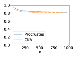
(a) $sim({\bm{A}},{\bm{B}})$

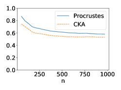
(b) $sim({\bm{A}},{\bm{C}})$

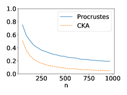
(c) $sim({\bm{A}},{\bm{D}})$

Figure 1: We compute CKA and Procrustes similarity scores with an increasing number of data examples $n$, and different similarity strength: ${\bm{B}}$ retains 80% of ${\bm{A}}$’s features, ${\bm{C}}$ 50%, and ${\bm{D}}$ 0%. Both metrics agree in (a) and (b), but Procrustes overestimates similarity in (c).

CKA ignores small changes in representations

When considering a sufficient number of data examples for both Procrustes and CKA, if two representations do not have dramatic differences (i.e., their 10% largest principal components are the same), CKA may overestimate similarity, while Procrustes remains stable, as observed by Ding et al. (2021).

Ensuring accurate analysis

Given the limitations previously mentioned, we take three remedial actions to guarantee that our analysis is as accurate as possible. Firstly, as both metrics will likely underestimate the similarity between different layer types, we will only discuss the variation of similarity when analysing such cases. For example, we will not compare $sim({\bm{A}},{\bm{B}})$ and $sim({\bm{A}},{\bm{C}})$ if ${\bm{A}}$ and ${\bm{B}}$ are convolutional layers but ${\bm{C}}$ is deconvolutional. We will nevertheless analyse the changes of $sim({\bm{A}},{\bm{C}})$ at different steps of training. Secondly, when both metrics disagree, we know that one of them is likely overestimating the similarity: Procrustes if the number of data examples is not sufficient, CKA if the difference between the two representations is not large enough.  Thus, we will always use the smallest of the two results for our interpretations.

2.4 Transfer learning

Transfer learning is the process of reusing knowledge learned from one or more source domains to improve the performance of a model on a target domain (Pan & Yang, 2009). Each domain $\mathcal{D}$ is composed of a feature space $\mathcal{X}$ and a marginal probability distribution $p({\bm{X}})$ where ${\bm{X}}=\{{\mathbf{x}}^{(i)}\}_{i=1}^{n}$ such that $\mathcal{D}\triangleq\{\mathcal{X},p({\bm{X}})\}$.

Types of transfer learning

Depending on the nature of the domains and considered tasks, transfer learning can be decomposed into multiple subcategories (see (Pan & Yang, 2009) for a detailed overview). In this study, we are interested in settings where the source and target domains are different but related and no classification or regression labels are available in the source domain. Following Pan & Yang (2009), this corresponds to self-taught learning (Raina et al., 2007) when the target domain contains labeled data and unsupervised learning otherwise.

Transfer learning with VAEs

Most of the research on transfer learning using VAEs focuses on how to efficiently perform transfer learning on specific applications. However, there is no clearly defined method to decide a priori which components should be retrained in which context. For example Lovrić et al. (2021) directly reuse the encoder learned on the source dataset in a target task on a different domain, Inoue et al. (2018) only retrain the encoder on the target domain, and Hung et al. (2019); Akrami et al. (2020) fine-tune the entire model. In Section 4.2, we will assess the specificity of the representations learned by VAEs using CKA. From this analysis, we will provide guidelines on which components should be retrained depending on the type of the target task. To assess whether transfer learning could be beneficial for a target task whose labels are known, we will also propose a method to visually identify shared latent variables between source and target domains.

3 Experimental setup

As stated in Section 1, the objectives of this experiment are 1) to estimate which components of the model would require retraining for the target task, and 2) to assess the transferability of the learned representations for self-taught transfer learning. To do so, in Section 4.1, we first ensure the chosen representational similarity metric is consistent with known facts about the learning dynamics of VAEs. Then, in Section 4.2, we assess the representational similarity of models learned on source and target domains when evaluated on target instances. Based on these observations, in Section 4.3 we provide some guidelines on which components to retrain depending on the target task, fulfilling our first objective. Then, we propose a method to visually identify shared variables between the source and target domain that are learned by VAEs, adressing our second objective. Finally, we confirm the validity of the visual analysis by comparing the observations with the results of classification on the target domain using latent representations learned from the source domain without any fine-tuning.

Learning objectives

We generally use vanilla VAEs except in Section 4.1, when comparing the representational similarity of models across different learning objectives and regularisation strength. In this case, we use learning objectives which allow for easy tuning of the ELBO’s regularisation strength, namely $\beta$-VAE (Higgins et al., 2017), $\beta$-TC VAE (Chen et al., 2018), Annealed VAE (Burgess et al., 2018), and DIP-VAE II (Kumar et al., 2018). A description of these methods can be found in Appendix E.  To provide fair and complementary insights into previous observations of such models (Locatello et al., 2019; Bonheme & Grzes, 2021), we will follow the experimental design of Locatello et al. (2019) regarding the architecture, learning objectives, and regularisation used. Moreover, disentanglement lib will be used as a codebase for our experiment. The complete details are available in Appendix C.

Datasets

For Section 4.1, we use three datasets which, based on the results of Locatello et al. (2019), are increasingly difficult for VAEs in terms of reconstruction loss: dSprites (Higgins et al., 2017), Cars3D (Reed et al., 2015), and SmallNorb (LeCun et al., 2004). For Section 4.2, we additionally use Symsol_reduced (Bonheme & Grzes, 2022) and Celeba (Liu et al., 2015) to create increaslingly challenging transfer learning configurations using the two pairs of datasets (dSprites, Symsol) and (Cars3D, Celeba).

Training process

For Section 4.1, we trained five models with different initialisations for 300,000 steps for each (learning objective, regularisation strength, dataset) triplet, and saved intermediate models to compare the similarity within individual models at different epochs. Appendix I explains our epoch selection methodology. We further trained five classical VAEs with different initialisations for 300,000 steps on Celeba and Symsol for Section 4.2.

Similarity measurement

For every dataset, we sampled 5,000 data examples, and we used them to compute all the similarity measurements. We compute the similarity scores between all pairs of layers of the different models following the different combinations outlined above. As Procrustes similarity takes significantly longer to compute compared to CKA (see below), we only used it to validate CKA results, restricting its usage to one dataset: Cars3D. We obtained similar results for the two metrics on Cars3D, thus we only reported CKA results in the main paper. Procrustes results can be found in Appendix F.

4 Results

In this section, we will discuss the similarity between models through the heatmaps obtained with CKA. The two models being compared will be described in the $x$ and $y$ axis, and the results will be averaged over 5 runs of each model. Specifically, given the $i^{th}$ run of two models $A_{i}$ and $B_{i}$ and their activations ${\bm{M}}_{j}^{A_{i}}$ and ${\bm{M}}_{j}^{B_{i}}$ over $n$ examples at layer $j$, the value displayed at the cell $(j,k)$ of the heatmap corresponds to the averaged CKA scores between the $j^{th}$ layer of $A$ and the $k^{th}$ layer of $B$:

$$CKA_{avg}({\bm{M}}_{j}^{A},{\bm{M}}_{k}^{B})=\frac{1}{25}\sum_{i=1}^{5}\sum_{l=1}^{5}CKA({\bm{M}}_{j}^{A_{i}},{\bm{M}}_{k}^{B_{l}}).$$ (6)

When describing these figures, we will refer to top-left (resp. bottom-right) quadrants to indicate the similarity scores between all the representations of the encoder (resp. decoder). This includes the off-diagonal CKA scores between layers of the same type. Similarly we will refer to the top-right (resp. bottom-left) quadrants when comparing the representations learned by the encoder and decoder of two models. Note that in this case, we will always dicuss the difference of scores between both models, (i.e., both quadrants will be compared). Indeed the layers of the encoder and decoder are of different type and discussing the scores obtained for only one quadrant without contrasting it with the other may be misleading as explained in Section 2.2.

4.1 Assessing the coherence of CKA scores with known facts about VAEs

The goal of this section is to verify that CKA can provide accurate information about the learning dynamics of VAEs. We thus check that the results observed using representational similarity are consistent with known facts about VAEs. Note that we obtained similar results using Procrustes similarity and fully connected neural network architectures, as reported in Appendices F and G.

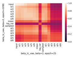
(a) Trained on Cars3D

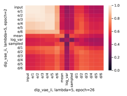
(b) Trained on dSprites

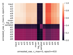
(c) Trained on SmallNorb

Figure 2: (a) shows the CKA similarity scores of activations at epochs 25 and 1090 of $\beta$-TC VAE trained on Cars3D with $\beta=2$. (b) shows the CKA similarity scores of activations at epochs 2 and 26 of DIP-VAE II trained on dSprites with $\lambda=5$. (c) shows the CKA similarity scores of activations at epochs 10 and 410 of Annealed VAE trained on SmallNorb with $c_{max}=5$.

Fact 1: the encoder is learned before the decoder

Using the information bottleneck (IB) theory, (Lee & Jo, 2021) have shown that in VAEs, the encoder is learned before the decoder. Moreover, this behaviour seems to be required for VAEs to learn meaningful representations as decoders which ignore the latent representations (e.g., because of posterior collapse or lagging inference) provide suboptimal reconstructions (Bowman et al., 2016; He et al., 2019). When comparing the representations learned at different epochs in Figure 2, we can see that CKA provides consistent results about this phenomenon: the encoder is learned first, and the representations of its layers become similar to the input after a few epochs (see the bright cells in the top-left quadrants in Figures 2(a), 2(b), and 2(c)). The decoder then progressively learns representations that gradually become closer to the input while the mean and variance representations are refined (see the dark cells in the bottom-right quadrant of Figures 2(a), 2(b), and 2(c)). Note that our choice of snapshots and snapshot frequency did not influence the results as verified in Appendices I and J.

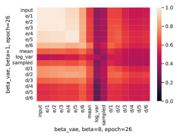
(a) $\beta$-VAE

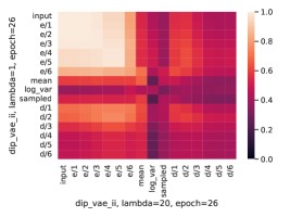
(b) DIP-VAE II

Figure 3: (a) shows the CKA similarity scores between the activations of two $\beta$-VAEs trained on dSprites with $\beta=1$, and $\beta=8$. (b) shows the CKA similarity scores between the activations of two DIP-VAE II trained on dSprites with $\lambda=1$, and $\lambda=20$. For both figures, the activations are taken after complete training.

Fact 2: very high regularisation leads to posterior collapse

It is well known that an excessively high pressure on the regularisation term of the ELBO in Equation 1 leads to posterior collapse (Dai & Wipf, 2018; Lucas et al., 2019a; b; Dai et al., 2020). When this happens, the sampled representation collapses to the prior — generally $\mathcal{N}({\bm{0}},{\bm{I}})$ — and the decoder has a poor reconstruction quality. This phenomenon is clearly visible with CKA in Figure 3. Indeed, the sampled representations of the collapsed model (dark line at the “sampled” column of Figures 3(a) and 3(b)) have a very low similarity with the representations learned by the encoder and decoder of a well-behaved model, in opposition to the sampled representation of a well-behaved model (lighter line at the “sampled” row of Figures 3(a) and 3(b)). This indicates that the collapsed sampled representations do not retain any information about the input, in opposition to any layer of a well-behaved model.

(a) Trained on Cars3D

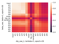
(b) Trained on dSprites

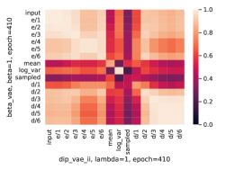
(c) Trained on SmallNorb

Figure 4: (a) shows the CKA similarity scores of activations of $\beta$-VAE and DIP-VAE II trained on Cars3D with $\beta=1$, and $\lambda=1$, respectively. (b) and (c) show the CKA similarity scores of the same learning objectives and regularisation strengths but trained on dSprites and SmallNorb.

Fact 3: encoders learn abstract features

It is not uncommon amongst practitioners to apply transfer learning to VAEs by using a pre-trained classifier as an encoder. The last layers (i.e., closest to the output and used for classification) are removed and replaced by the mean and variance layers. The assumption, which underlies transfer learning, is that encoders learn abstract features which are shared with other types of network (Yosinski et al., 2014; Bansal et al., 2021; Csiszárik et al., 2021). The results of CKA are also in line with this fact. Indeed, the bright top-left quadrants of Figures 4(a), 4(b), and 4(c), indicate that encoders of VAEs trained using different learning objectives are highly similar. This observation holds when comparing encoders and classifiers with equivalent architectures (see Appendix H).

4.2 The representational similarity of VAEs trained on different domains

We have seen in Section 4.1 that the representations learned by the encoder of VAEs with different learning objectives and by classifiers with the same architecture were similar except for the mean and variance representations. Thus, encoders can be thought of as generic feature extractors. In this section, we are going one step further and study how transferable the representations learned by VAEs are between domains. Specifically, how the representations learned on different but related domains differ and how this informs the potential of VAEs for transfer learning.

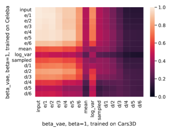
(a) No fine-tuning.

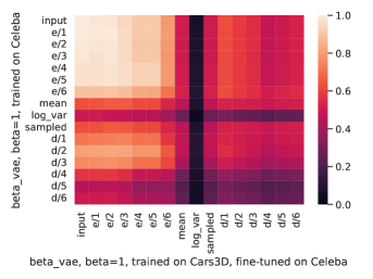
(b) Mean and variance are retrained.

Figure 5: Both figures show CKA similarity scores between the activations of two VAEs evaluated on the target dataset ${\bm{X}}_{t}=$ Celeba but trained on different datasets. The models on the x-axis are trained on ${\bm{X}}_{s}=$ Cars3D while the models on the y-axis are trained on the target dataset ${\bm{X}}_{t}=$ Celeba. In (a) the model on the x-axis is evaluated on Celeba without any fine-tuning, in (b) its mean and variance are retrained on Celeba beforehand.

Encoders learn generic representations

When assessed on a target dataset ${\bm{X}}_{t}$, the representations learned by an encoder trained on a source dataset ${\bm{X}}_{s}$ retain a high similarity with those obtained from a VAE directly trained on ${\bm{X}}_{t}$, as demonstrated by the bright top-left quadrants of Figure 5(a). In fact the similarity is as high as what is observed on encoders trained on the same dataset in Figure 4. This shows that before the mean and variance layers, the encoders extract features that are sufficiently abstract to be shared between domains (e.g., curves, edges, frequencies) (Yosinski et al., 2014; Sharif Razavian et al., 2014). Indeed, the source and target images are very different and a high specificity of the features encoded would lower the similarity score.

Decoders learn specific representations

In opposition to the general domain-independent representations of encoders, the dark bottom-right quadrant of Figure 5(a) shows that the decoder’s representations are very different if they were initially trained on the source or target dataset. One could argue that decoders also learn generic features but have different activations because the input ${\mathbf{z}}$ is different between the models. However, after retraining the mean and sampled representations of a VAE trained on the source domain, in Figure 5(b) we still obtain a bottom-right quadrant noticeably darker than for decoders trained on the same dataset in Figure 4, indicating that in opposition to encoders’ representations, decoders’ representations are far more specific to the dataset on which they were trained.

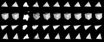
(a) Fixed encoder

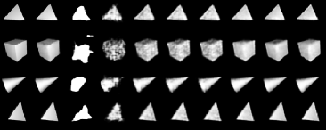
(b) Retrained mean and variance

Figure 6: (a) and (b) show the reconstruction of images from ${\bm{X}}_{t}=$ Symsol by a VAE trained on ${\bm{X}}_{s}=$ dSprites. The first two columns on the left are the original images and reconstruction from a model trained on ${\bm{X}}_{t}$, respectively. From left to right, columns 3 to 10 show the reconstruction as we progressively unfreeze and retrain the decoder layers, starting from layers closer to the input. The mean and variance layers of the encoder are fixed in (a) but retrained in (b).

4.3 Implications for transfer learning

Implications for unsupervised transfer learning

As we have seen with CKA, decoders’ representations are specific. Thus the decoder of a VAE trained on a source domain will need to be retrained to generate images on the target domain. We show in Figure 6 that the more layers of the decoder are retrained, the better the reconstruction. Thus, the specificity of the representations learned by the decoder holds for all the layers, not only a subset of them. Furthermore, the similar outputs obtained in Figures 6(a) and 6(b) show that retraining the latent representation has no impact on the reconstruction quality compared to the number of retrained layers of the decoder. We can thus conclude that for image generation on the target domain, one can freeze the encoder entirely during transfer but needs to retrain most of the layers of the decoder.

Implications for self-taught transfer learning

Assessing the implications of our analysis of representational similarity for supervised target tasks is less straightforward than for reconstruction. Indeed, while we can directly use the similarity between the representations learned by a decoder trained on the source domain and its counterpart trained on the target domain in the context of image generation, a similar approach would be unreliable for supervised target tasks. Let us consider the mean representation of a model trained on the source domain, ${\bm{\mu}}(\cdot;{\bm{\phi}}_{s})$, and the mean representation of a model trained on the target domain, ${\bm{\mu}}(\cdot;{\bm{\phi}}_{t})$. The transferability of ${\bm{\mu}}(\cdot;{\bm{\phi}}_{s})$ to the target domain does not depend on how similar ${\bm{\mu}}({\bm{X}}_{t};{\bm{\phi}}_{s})$ is to ${\bm{\mu}}({\bm{X}}_{t};{\bm{\phi}}_{t})$, but on how informative the shared latent representations are about the task labels ${\mathbf{y}}_{t}$. For example, let us consider a simple classification task with only one binary label (i.e., ${\mathbf{y}}_{t}\in\{0,1\}$). One could have a very high similarity between ${\bm{\mu}}({\bm{X}}_{t};{\bm{\phi}}_{s})$ and ${\bm{\mu}}({\bm{X}}_{t};{\bm{\phi}}_{t})$ because both representations share many variables which are useful for reconstruction. However, ${\bm{\mu}}({\bm{X}}_{t};{\bm{\phi}}_{s})$ may not encode the most informative variable about ${\mathbf{y}}_{t}$, which would lead to poor results on the target task. Inversely, one could have a very low similarity between ${\bm{\mu}}({\bm{X}}_{t};{\bm{\phi}}_{s})$ and ${\bm{\mu}}({\bm{X}}_{t};{\bm{\phi}}_{t})$ with ${\bm{\mu}}({\bm{X}}_{t};{\bm{\phi}}_{s})$ encoding only the most informative variable about ${\mathbf{y}}_{t}$, which would lead to good results on the target task. Despite this, one can still use knowledge from representational similarity to assess the transferability of latent representations to a supervised target task, albeit in a different way. We know that encoders’ representations are generic. Thus, if a common variable is shared between the source and target domains, it should be encoded in a similar way regardless of the domain of the input. For example, if colours are encoded on a VAE trained on the source domain, they should also be encoded by ${\bm{\mu}}({\bm{X}}_{t};{\bm{\phi}}_{s})$. Furthermore, we know from representational similarity that the decoder learns specific representations. It means that given any ${\bm{\mu}}(\cdot;{\bm{\phi}}_{s})$, it should provide a likely reconstruction in the target domain. Hence, akin to paired inputs in multimodal datasets, the decoder should provide an approximation of any target example ${\mathbf{x}}_{t}^{(i)}$ in the source domain. One could thus identify the shared latent variables between the source and target domain by visually comparing the target examples and their reconstruction in the source domain.

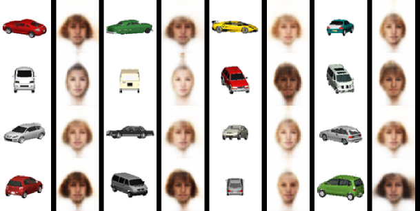
Figure 7: Reconstruction of Cars3D images using a VAE trained on Celeba. The black borders on the reconstructed images are due to the presence of similar borders in Celeba images.

Case study 1: Celeba to cars3D

To validate our hypothesis, we will use Figure 7 to compare the samples from Cars3D with their reconstruction using a VAE trained on Celeba. One can clearly see that Celeba and Cars3d display a common variable colour: cars with light colours lead to faces with light hair and skin in the source domain while cars of darker colour are linked with faces with darker hair and skin. In the same way, we can identify a shared variable width: the profile views of cars lead to faces with wider jaw and haircut than front views of cars which results in faces with fine jaw and tight haircuts. The labels of the target classification task are object type, elevation, and azimuth which are only loosely related to the shared variables identified. We can thus hypothesise that despite the observed shared variables, the performances on the target classification task will likely drop when using the representations learned on Cars3D.

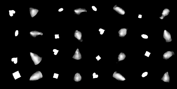
Figure 8: Reconstruction of dSprites images using a VAE trained on Symsol

Case study 2: Symsol to dSprites

Taking a second example where we transfer representations from Symsol to dSprites in Figure 8, we can identify several shared variables: position x and y, as the reconstructed output is displayed in the same area as the input for all the examples; size, albeit less consistently, as larger sprites generally result in larger reconstructed outputs (e.g. see the two squares on the last row); rotation, to a lower extent, as the output tends to be slanted when the input is rotated but the angle of rotation between input and reconstruction generally do not coincide. We can also see that there is no shared variable for the shape. Indeed, different sprites have sometimes a more similar reconstruction shape than the sprites of different types (e.g., see the heart and square in rows 3-4 and columns 1-2, and the square in row 4, columns 3-4). The labels of the target classification task are shape, scale, rotation, x and y position. We have seen that x and y positions were clearly shared variables so we can expect good accuracy on the classification of these labels. Scale and rotation were also identified but in a less consistent fashion. We can thus hypothesise a small drop in accuracy when using representations learned on Symsol for these classifications. Finally, shape was definitely not a shared variable and we should expect a more important drop in accuracy for the classification of this label.

Table 1: Averaged classification accuracy of a Gradient Boosted Tree on the target domain using the mean representations of VAEs trained on the source and target domain. All the results are averaged over 5 seeds.

Target domain	Source domain	Accuracy (avg.)
dSprites	dSprites	0.40
dSprites	Symsol	0.39
Symsol	Symsol	1.0
Symsol	dSprites	0.99
Celeba	Celeba	0.83
Celeba	Cars3D	0.82
Cars3D	Cars3D	0.59
Cars3D	Celeba	0.42

How well do these observations correlate with target task performances?

Overall we can see in Table 1 that the performances using representations learned on the source domains are on par with the results obtained with representations learned from the target domain with the exception of ${\bm{X}}_{s}=$ Celeba and ${\bm{X}}_{t}=$ Cars3D. To avoid clutter, the accuracy scores in Table 1 are averaged over all the labels and the accuracy by label is detailed in Appendix A. Looking into the results obtained for individual labels of the classification on dSprites using representations learned on Symsol, the second case study in this section, we observe the largest drop for shape classification (0.19), followed by smaller drops in rotation and scaling (around 0.05 for both), which is consistent with our preliminary observations. Interestingly, this is compensated by a gain in accuracy of 0.15 for x and y positions which were the most noticeable shared variables. While not studied visually, classification on Celeba using representations learned on Cars3D shows similar results to those obtained with representations learned on Celeba on most labels. The accuracy decreases mainly for attributes which intuitively cannot be inferred from car representations such as smiling, wearing makeup, or being male. The lower performances of ${\bm{X}}_{s}=$ Celeba and ${\bm{X}}_{t}=$ Cars3D are coherent with our analysis of the corresponding first case study in this section. The shared variables were not very informative about the labels and the classification accuracy evenly dropped by 0.13 to 0.19 across all the labels.

5 Conclusion

After ensuring that CKA was consistent with known behaviours of VAEs in Section 4.1, we used this metric in Section 4.2 to show that encoders’ representations are generic but decoders’ specific. In Section 4.3 we further studied the implications of this analysis for transfer learning.

Impact on unsupervised transfer learning

When the target task is image generation, because the decoder learns specific representations, one needs to retrain most of its layers to obtain a good reconstruction. However, as the encoder learns generic representations, it does not need to be retrained.

Impact on self-taught transfer learning

Using the fact that encoders’ representations are generic, we hypothesised that when provided with an input from the target domain, a VAE trained on a source domain will retain the shared variables between both domains in its latent representations. Furthermore, due to the specificity of decoders’ representations, any target example will be reconstructed in the source domain using these shared variables. Thus, by visually comparing inputs from the target domain and outputs from a VAE trained on a different source domain, one can identify the shared variables learned by this model. We have seen that such analysis is very informative on the transferability of the latent representations to target classification tasks. Indeed, clearly identified shared variables, when related to the classification labels, lead to equivalent or better results when using latents obtained from an encoder learned on a different source domain. This finding can have implications in practical applications where one can only obtain a few samples from the target domain but a large dataset is available from a source domain.

Ethical statement

While the methods proposed in this paper open avenues for greener transfer learning of VAEs, this experiment still required extensive computations. We trained more than 300 VAEs using 4 learning objectives, 5 different initialisations, 5 regularisation strengths, and 3 datasets, which took around 6,000 hours on an NVIDIA A100 GPU. We then computed the CKA scores for the 15 layer activations (plus the input) of each model combinations considered above at 5 different epochs, resulting in 470 million similarity scores and approximately 7,000 hours of computation on an Intel Xeon Gold 6136 CPU. As Procrustes is slowed down by the computation of the nuclear norm for high dimensional activations, the same number of similarity scores would have been prohibitively long to compute, requiring 30,000 hours on an NVIDIA A100 GPU. We thus only computed the Procrustes similarity for one dataset, reducing the computation time to 10,000 hours. Overall, based on the estimations of Lacoste et al. (2019), the computations done for this experiment amount to 2,200 Kg of $\mathrm{CO_{2}}$, which corresponds to the $\mathrm{CO_{2}}$ produced by one person over 5 months. To mitigate the negative environmental impact of our work, we released all our trained models and metric scores at https://data.kent.ac.uk/428/, and https://data.kent.ac.uk/444/, respectively. We hope that this will help to prevent unnecessary recomputation should others wish to reuse our results. Moreover, we believe that our findings could help practitioners to pre-select likely candidate models for transfer learning and avoid unnecessary retraining, reducing $\mathrm{CO_{2}}$ emissions in the future.

Acknowledgments

The authors thank Frances Ding for an insightful discussion on the Procrustes distance, as well as Théophile Champion and Declan Collins for their helpful comments on the paper.

Appendix A Accuracy of classification tasks detailed per label

This section details the accuracy per label of the classification tasks presented in Table 1 of Section 4.3. Note that Symsol is omitted because the classification task has only one label.

Table 2: Averaged classification accuracy of a Gradient Boosted Tree on the Cars3D using the mean representations of VAEs trained on different source domains. All the results are averaged over 5 seeds.

Source domain	Elevation	Azimuth	Object type
Cars3d	0.69	0.73	0.35
Celeba	0.50	0.60	0.16

Table 3: Averaged classification accuracy of a Gradient Boosted Tree on the dSprites using the mean representations of VAEs trained on different source domains. All the results are averaged over 5 seeds.

Source domain	Shape	Scale	Orientation	x position	y position
dSprites	0.72	0.53	0.11	0.31	0.31
Symsol	0.52	0.48	0.05	0.46	0.45

Table 4: Averaged classification accuracy of a Gradient Boosted Tree on the Celeba using the mean representations of VAEs trained on different source domains. As CelebA has 40 labels, only those with a difference in accuracy higher than $0.01$ between source domains are reported for readability. All the results are averaged over 5 seeds.

Label	Source domain	Accuracy
Attractive	Celeba	0.68
Attractive	Cars3D	0.64
Blond Hair	Celeba	0.89
Blond Hair	Cars3D	0.87
Heavy Makeup	Celeba	0.74
Heavy Makeup	Cars3D	0.68
High Cheekbones	Celeba	0.62
High Cheekbones	Cars3D	0.59
Male	Celeba	0.75
Male	Cars3D	0.67
Smiling	Celeba	0.63
Smiling	Cars3D	0.60
Wavy Hair	Celeba	0.72
Wavy Hair	Cars3D	0.70
Wearing Lipstick	Celeba	0.75
Wearing Lipstick	Cars3D	0.67

Appendix B Additional figures obtained when retraining the outermost layers of the decoder first

This section provides complementary observations to Figure 6 when we unfreeze the outermost layers of the decoder first. As in Figure 6 the more layers of the decoder are retrained, the better the reconstruction. The similar outputs obtained in Figures 9(a) and 9(b) show that retraining the latent representation has no impact on the reconstruction quality compared to the number of retrained layers of the decoder.

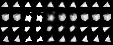
(a) Fixed encoder

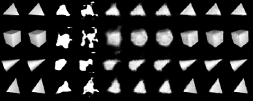
(b) Retrained mean and variance

Figure 9: (a) and (b) show the reconstruction of Symsol images by a VAE trained on dSprites. The first two columns on the left are the original images and reconstruction from a model trained on the target dataset, respectively. From left to right, columns 3 to 10 show the reconstruction as we progressively unfreeze and retrain the decoder layers, starting from layers closer to the output. The mean and variance layers of the encoder are fixed in (a) but retrained in (b).

Appendix C Experimental setup

To facilitate the reproducibility of our experiment, we detail below the Procrustes normalisation process and the configuration used for model training.

Procrustes normalisation

Similarly to Ding et al. (2021), given an activation matrix ${\bm{X}}\in\mathbb{R}^{n\times m}$ containing $n$ samples and $m$ features, we compute the vector $\bar{{\bm{x}}}\in\mathbb{R}^{m}$ containing the mean values of the columns of ${\bm{X}}$. Using the outer product $\otimes$, we get $\bar{{\bm{X}}}={\bm{1}}_{n}\otimes\bar{{\bm{x}}}$, where ${\bm{1}}_{n}\in\mathbb{R}^{n}$ is a vector of ones and $\bar{{\bm{X}}}\in\mathbb{R}^{n\times m}$. We then normalise ${\bm{X}}$ such that

$$\dot{{\bm{X}}}=\frac{{\bm{X}}-\bar{{\bm{X}}}}{\lVert{\bm{X}}-\bar{{\bm{X}}}\rVert_{F}}.$$ (7)

As the Frobenius norm of $\dot{{\bm{X}}}$ and $\dot{{\bm{Y}}}$ is 1, and $\lVert\dot{{\bm{Y}}}^{T}\dot{{\bm{X}}}\rVert_{*}$ is always positive (1 when $\dot{{\bm{X}}}=\dot{{\bm{Y}}}$, smaller otherwise), Equation 4 lies in $[0,2]$, and Equation 5 in $[0,1]$.

VAE training

Our implementation uses the same hyperparameters as Locatello et al. (2019), and the details are listed in Table 5 and 6. We reimplemented Locatello et al. (2019) code base, designed for Tensorflow 1, in Tensorflow 2 using Keras. The model architecture used is also identical, as described in Table 7. Each model is trained 5 times, on seeded runs with seed values from 0 to 4. Intermediate models are saved every 1,000 steps for SmallNorb, 6,000 steps for Cars3D and 11,520 steps for dSprites. Every image input is normalised to have pixel values between 0 and 1.

For the fully-connected models presented in Appendix G, we used the same architecture and hyperparameters as those implemented in disentanglement lib of Locatello et al. (2019), and the details are presented in Table 8 and 9.

Table 5: Shared hyperparameters

Parameter	Value
Batch size	64
Latent space dimension	10
Optimizer	Adam
Adam: $\beta_{1}$	0.9
Adam: $\beta_{2}$	0.999
Adam: $\epsilon$	1e-8
Adam: learning rate	0.0001
Reconstruction loss	Bernoulli
Training steps	300,000
Intermediate model saving	every 6K steps
Train/test split	90/10

Table 6: Model-specific hyperparameters

Model	Parameter	Value
$\beta$-VAE	$\beta$	[1, 2, 4, 6, 8]
$\beta$-TC VAE	$\beta$	[1, 2, 4, 6, 8]
DIP-VAE II	$\lambda_{od}$	[1, 2, 5, 10, 20]
	$\lambda_{d}$	$\lambda_{od}$
Annealed VAE	$C_{max}$	[5, 10, 25, 50, 75]
	$\gamma$	1,000
	iteration threshold	100,000

Table 7: Shared architecture

Encoder	Decoder
Input: $\mathbb{R}^{64\times 63\times channels}$	$\mathbb{R}^{10}$
Conv, kernel=4×4, filters=32, activation=ReLU, strides=2	FC, output shape=256, activation=ReLU
Conv, kernel=4×4, filters=32, activation=ReLU, strides=2	FC, output shape=4x4x64, activation=ReLU
Conv, kernel=4×4, filters=64, activation=ReLU, strides=2	Deconv, kernel=4×4, filters=64, activation=ReLU, strides=2
Conv, kernel=4×4, filters=64, activation=ReLU, strides=2	Deconv, kernel=4×4, filters=32, activation=ReLU, strides=2
FC, output shape=256, activation=ReLU, strides=2	Deconv, kernel=4×4, filters=32, activation=ReLU, strides=2
FC, output shape=2x10	Deconv, kernel=4×4, filters=channels, activation=ReLU, strides=2

Table 8: Fully-connected architecture

Encoder	Decoder
Input: $\mathbb{R}^{64\times 63\times channels}$	$\mathbb{R}^{10}$
FC, output shape=1200, activation=ReLU	FC, output shape=256, activation=tanh
FC, output shape=1200, activation=ReLU	FC, output shape=1200, activation=tanh
FC, output shape=2x10	FC, output shape=1200, activation=tanh

Table 9: Hyperparameters of fully-connected models

Model	Parameter	Value
$\beta$-VAE	$\beta$	[1, 8, 16]
$\beta$-TC VAE	$\beta$	[2]
DIP-VAE II	$\lambda_{od}$	[1, 20, 50]
	$\lambda_{d}$	$\lambda_{od}$
Annealed VAE	$C_{max}$	[5]
	$\gamma$	1,000
	iteration threshold	100,000

Appendix D Resources

As mentioned in Sections 1 and 3, we released the code of our experiment, the pre-trained models and similarity scores of Section 4.1:

• The similarity scores can be downloaded at https://data.kent.ac.uk/444/

• The pre-trained models can be downloaded at https://data.kent.ac.uk/428/

• The code is available at https://github.com/bonheml/VAE_learning_dynamics

Note that the 300 VAE models released correspond to models trained with:

• 4 different learning objectives,

• 5 initialisations,

• 3 datasets,

• 5 regularisation strengths.

Appendix E Disentangled representation learning

As mentioned in Section 2, we are interested in the family of methods modifying the weight on the regularisation term of Equation 1 to encourage disentanglement. In our paper, the term regularisation refers to the moderation of this parameter only. To achieve this, our experiment will focus on the models described below.

$\beta$-VAE

The goal of this method (Higgins et al., 2017) is to penalise the regularisation term of Equation 1 by a factor $\beta>1$, such that

$$\operatorname{\mathcal{L}({\bm{\theta}},{\bm{\phi}};{\mathbf{x}})}=\mathbb{E}_{q_{{\bm{\phi}}}({\mathbf{z}}|{\mathbf{x}})}\left[\log p_{{\bm{\theta}}}({\mathbf{x}}|{\mathbf{z}})\right]-\beta D_{\mathrm{KL}}\left(q_{{\bm{\phi}}}({\mathbf{z}}|{\mathbf{x}})\;\middle\|\;p({\mathbf{z}})\right).$$ (8)

Annealed VAE

Burgess et al. (2018) proposed to gradually increase the encoding capacity of the network during the training process. The goal is to progressively learn latent variables by decreasing order of importance. This leads to the following objective, where C is a parameter that can be understood as a channel capacity and $\gamma$ is a hyper-parameter penalising the divergence, similarly to $\beta$ in $\beta$-VAE:

$$\operatorname{\mathcal{L}({\bm{\theta}},{\bm{\phi}};{\mathbf{x}})}=\mathbb{E}_{q_{{\bm{\phi}}}({\mathbf{z}}|{\mathbf{x}})}\left[\log p_{{\bm{\theta}}}({\mathbf{x}}|{\mathbf{z}})\right]-\gamma\left|D_{\mathrm{KL}}\left(q_{{\bm{\phi}}}({\mathbf{z}}|{\mathbf{x}})\;\middle\|\;p({\mathbf{z}})\right)-\mathrm{C}\right|.$$ (9)

As the training progresses, the channel capacity $\mathrm{C}$ is increased, going from zero to its maximum channel capacity $\mathrm{C_{max}}$ and allowing a higher value of the KL divergence term. VAEs that use Equation 9 as a learning objective are referred to as Annealed VAEs in this paper.

$\beta$-TC VAE

Chen et al. (2018) argued that only the distance between the estimated latent factors and the prior should be penalised to encourage disentanglement, such that

$$\operatorname{\mathcal{L}({\bm{\theta}},{\bm{\phi}};{\mathbf{x}})}=\mathbb{E}_{p({\mathbf{x}})}\left[\mathbb{E}_{q_{{\bm{\phi}}}({\mathbf{z}}|{\mathbf{x}})}\left[\log p_{{\bm{\theta}}}({\mathbf{x}}|{\mathbf{z}})\right]-D_{\mathrm{KL}}\left(q_{{\bm{\phi}}}({\mathbf{z}}|{\mathbf{x}})\;\middle\|\;p({\mathbf{z}})\right)\right]\\ -\lambda D_{\mathrm{KL}}\left(q_{{\bm{\phi}}}({\mathbf{z}})\;\middle\|\;p({\mathbf{z}})\right).$$ (10)

Here, $D_{\mathrm{KL}}\left(q_{{\bm{\phi}}}({\mathbf{z}})\;\middle\|\;p({\mathbf{z}})\right)$ is approximated by penalising the dependencies between the dimensions of $q_{{\bm{\phi}}}({\mathbf{z}})$:

$$\operatorname{\mathcal{L}({\bm{\theta}},{\bm{\phi}};{\mathbf{x}})}\approx\frac{1}{n}\sum_{i=1}^{n}\left[\mathbb{E}_{q_{{\bm{\phi}}}({\mathbf{z}}|{\mathbf{x}}^{(i)})}\left[\log p_{{\bm{\theta}}}({\mathbf{x}}^{(i)}|{\mathbf{z}})\right]-D_{\mathrm{KL}}\left(q_{{\bm{\phi}}}({\mathbf{z}}|{\mathbf{x}}^{(i)})\;\middle\|\;p({\mathbf{z}})\right)\right]\\ -\underbrace{\lambda D_{\mathrm{KL}}\left(q_{{\bm{\phi}}}({\mathbf{z}})\;\middle\|\;\prod_{j=1}^{\mathrm{D}}q_{{\bm{\phi}}}({\mathbf{z}}_{j})\right)}_{\textrm{total correlation}}.$$ (11)

The total correlation of Equation 11 is then approximated over a mini-batch of samples $\{{\mathbf{x}}^{(i)}\}_{i=1}^{m}$ as follows:

$$\mathbb{E}_{q_{{\bm{\phi}}}({\mathbf{z}})}[\log{q_{{\bm{\phi}}}({\mathbf{z}})}]\approx\frac{1}{m}\sum_{i=1}^{m}\left(\log\frac{1}{nm}\sum_{k=1}^{m}q_{{\bm{\phi}}}({\mathbf{z}}^{(i)}|{\mathbf{x}}^{(k)})\right),$$ (12)

where $m$ is the number of samples in the mini-batch, and $n$ total number of input examples. $\mathbb{E}_{q_{{\bm{\phi}}}({\mathbf{z}}_{j})}[\log{q_{{\bm{\phi}}}({\mathbf{z}}_{j})}]$ can be computed in a similar way. We refer the reader to (Chen et al., 2018, Appendix C.1) for the detailed derivation of Equation 12.

DIP-VAE

Similarly to Chen et al. (2018), Kumar et al. (2018) proposed to regularise the distance between $q_{\bm{\phi}}({\mathbf{z}})$ and $p({\mathbf{z}})$ using Equation 10. The main difference is that here $D_{\mathrm{KL}}\left(q_{{\bm{\phi}}}({\mathbf{z}})\;\middle\|\;p({\mathbf{z}})\right)$ is measured by matching the moments of the learned distribution $q_{{\bm{\phi}}}({\mathbf{z}})$ and its prior $p({\mathbf{z}})$. The second moment of the learned distribution is given by

$$\mathrm{Cov}_{q_{{\bm{\phi}}}({\mathbf{z}})}[{\mathbf{z}}]=\mathrm{Cov}_{p({\mathbf{x}})}\left[\mu_{{\bm{\phi}}}({\mathbf{x}})\right]+\mathbb{E}_{p({\mathbf{x}})}\left[\Sigma_{{\bm{\phi}}}({\mathbf{x}})\right].$$ (13)

DIP-VAE II penalises both terms of Equation 13 such that

$$\lambda D_{\mathrm{KL}}\left(q_{{\bm{\phi}}}({\mathbf{z}})\;\middle\|\;p({\mathbf{z}})\right)=\lambda_{od}\sum_{i\neq j}\left(\mathrm{Cov}_{q_{{\bm{\phi}}}({\mathbf{z}})}\left[{\mathbf{z}}\right]\right)_{ij}^{2}+\lambda_{d}\sum_{i}\left(\mathrm{Cov}_{q_{{\bm{\phi}}}({\mathbf{z}})}\left[{\mathbf{z}}\right]_{ii}-1\right)^{2},$$

where $\lambda_{d}$ and $\lambda_{od}$ are the penalisation terms for the diagonal and off-diagonal values respectively.

Appendix F Consistency of the results with Procrustes Similarity

As mentioned in Section 3, in this section we provide a comparison between the CKA scores reported in the main paper, and the Procrustes scores for the Cars3D dataset. We can see in Figures 10 to 12 that Procrustes and CKA provide similar results.  Figures 10 and 11 show that Procrustes tends to overestimate the similarity between high-dimensional inputs, as mentioned in Section 2.3 (recall the example given in Figure 1). In Figure 12, we observe a slightly lower similarity with Procrustes than CKA on the $5^{th}$ and $6^{th}$ layers of the encoder, indicating that some small changes in the representations may have been underestimated by CKA, as discussed in Section 2.3 and by Ding et al. (2021). Note that the difference between the CKA and Procrustes similarity scores in Figure 12 remains very small (around 0.1) indicating consistent results between both metrics.

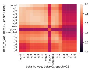
(a) CKA

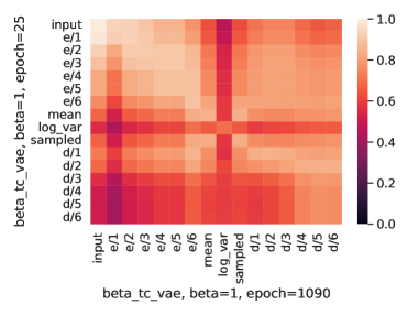
(b) Procrustes

Figure 10: (a) shows the CKA similarity scores of activations at epochs 25 and 1090 of $\beta$-TC VAE trained on Cars3D with $\beta=2$. (b) shows the Procrustes similarity scores of the same configuration. We observe the same trend with both metrics with Procrustes slightly overestimating the similarity between high dimensional activations (bottom-right quadrants), which agrees with the properties of the Procrustes similarity reported in Section 2.3.

(a) CKA

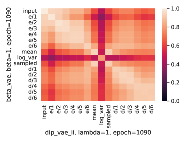
(b) Procrustes

Figure 11: (a) shows the CKA similarity scores of activations of $\beta$-VAE and DIP-VAE II trained on Cars3D with $\beta=1$, and $\lambda=1$, respectively. (b) shows the Procrustes similarity scores using the same configuration. We observe the same trend with both metrics with Procrustes slightly overestimating the similarity between high dimensional activations (bottom-right quadrants) (c.f. Section 2.3).

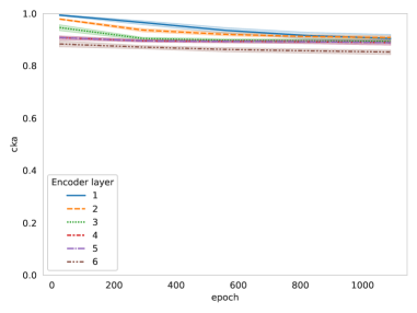
(a) CKA for $\beta=1$

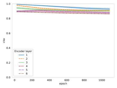
(b) CKA for $\beta=8$

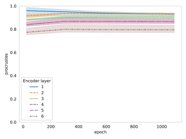
(c) Procrustes for $\beta=1$

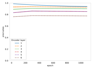
(d) Procrustes for $\beta=8$

Figure 12: (a) shows the CKA scores between the inputs and the activations of the first 6 layers of the encoder of a $\beta$-VAE trained on Cars3D with $\beta=1$. (b) shows the scores between the same representations with $\beta=8$. (c) and (d) are the Procrustes scores of the same configurations. We observe the same trend for both metrics with more variance in (c) for Procrustes with $\beta=1$. Procrustes also displays a slightly lower similarity for layers 4 to 6 of the encoder, possibly due to changes in the representation that are underestimated by CKA (c.f. Section 2.3).

Appendix G CKA on fully-connected architectures

In order to assess the generalisability of our findings, we have repeated our observations on the fully-connected VAEs that are described in Appendix C. We can see in Figures 13, 14, and 15 that the same general trend as for the convolutional architectures can be identified.

Learning in fully-connected VAEs is also bottom-up

We can see in Figure 13 that, similarly to the convolutional architectures shown in Figure 2, the encoder is learned early in the training process. Indeed between epochs 1 and 10, the encoder representations become highly similar to the representations of the fully trained model (see Figures 13(a) and 13(b)). The decoder is then learned with its representational similarity with the fully trained decoder raising after epoch 10 (see Figure 13(c)).

Impact of regularisation

As in convolutional architectures shown in Figure 3, the variance and sampled representations retain little similarity with the encoder representations in the case of posterior collapse, as shown in Figure 14. Interestingly, in fully-connected architectures the decoder retains more similarity with its less regularised version than in convolutional architectures, despite suffering from poor reconstruction when heavily regularised. Thus, CKA of the representations of fully-connected decoders may not be a good predictor of reconstruction quality.

Impact of learning objective

Figure 15 provides results similar to the convolutional VAEs observed in Figure 4, with a very high similarity between encoder layers learned from different learning objectives (see diagonal values of the upper-left quadrant). Here again, the representational similarity of the decoder seems to vary depending on the dataset, even though this is less marked than for convolutional architectures. We can also see that the representational similarity between different layers of the encoder vary depending on the dataset, which was less visible in convolutional architectures. For example, the similarity between the first and subsequent layers of the encoder in SmallNorb is much lower in fully-connected VAEs. Given that SmallNorb is a hard dataset to learn for VAEs (Locatello et al., 2019), one could hypothesise that the encoder of fully-connected VAE, being less powerful, is unable to retain as much information as its convolutional counterpart, leading to lower similarity scores with the representations of the first encoder layer.

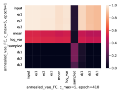
(a) Epoch 1

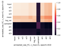
(b) Epoch 10

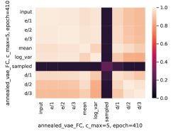
(c) Epoch 410

Figure 13: (a), (b), and (c) show CKA scores between a fully-trained fully-connected Annealed VAE and a fully-connected Annealed VAE trained for 1, 10 and 410 epochs, respectively. All the models are trained on SmallNorb and the results are averaged over 5 seeds. As in Figure 2 of Section 4.1, we can see that there is a high similarity between the representations learned by the encoder early in the training and after complete training (see the bright cells in the top-left quadrants in (a), (b), and (c)). The mean and variance representations similarity with a fully trained model increase after a few more epochs (the purple line in the middle disappear between (a) and (b)), and finally the decoder is learned (see bright cells in bottom-right quadrant of (c)).

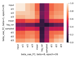
(a) $\beta=8$

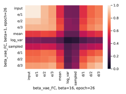
(b) $\beta=16$

Figure 14: (a) and (b) show the representational similarity between fully-connected $\beta$-VAEs trained with $\beta=1$, and fully-connected $\beta$-VAEs trained with $\beta=8$ and $\beta=16$, respectively. All models are trained on dSprites and the scores are averaged over 5 seeds. In both figures, the encoder representations stay very similar (bright cells in the top-left quadrants), except for the mean, variance and sampled representations. While the variance representation is increasingly different as we increase $\beta$, the decoder does not show the dramatic dissimilarity observed in convolutional architectures in Figure 3.

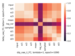
(a) Trained on Cars3D

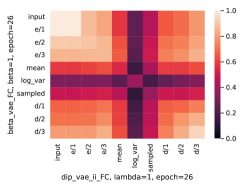
(b) Trained on dSprites

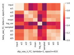
(c) Trained on SmallNorb

Figure 15: (a) shows the CKA similarity scores of activations of $\beta$-VAE and DIP-VAE II with fully-connected architectures trained on Cars3D with $\beta=1$, and $\lambda=1$, respectively. (b) and (c) show the CKA similarity scores of the same learning objectives and regularisation strengths but trained on dSprites and SmallNorb. All the results are averaged over 5 seeds. We can see that the representational similarity of all the layers of the encoder (top-left quadrant) except mean and variance is high (CKA $\geqslant 0.8$). However, as in Figure 4, the mean, variance, sampled (center diagonal values), and decoder (bottom-right quadrants) representational similarity of different learning objectives seems to vary depending on the dataset. In (a) and (c) they have high similarity, while in (b) the similarity is lower. Moreover, in (c) the input and first layer of the encoder are quite distinct from the other representations, which was not the case in convolutional architectures.

Appendix H How similar are the representations learned by encoders and classifiers?

To compare VAEs with classifiers, we used the convolutional architecture of an encoder for classification, replacing the mean and variance layers by the final classifier layers. As shown in Figure 16, we obtain a high representational similarity when comparing VAEs and classifiers indicating, consistently with the observations of Yosinski et al. (2015), that classifiers seem to learn generative features. This explains why encoders based on pre-trained classifier architectures such as VGG have empirically demonstrated good performances (Liu et al., 2021) and also suggests that the weights of the pre-trained architecture could be used as-is without further updates. This also indicates that using pre-trained encoders may be beneficial in the context of transfer learning, domain adaptation (Pan & Yang, 2009), or simply reconstruction quality (Liu et al., 2021) which is consistent with our results in Section 4.2.

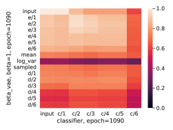
(a) Trained on Cars3D

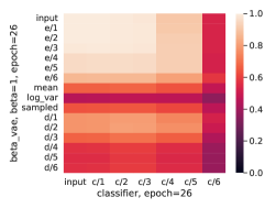
(b) Trained on dSprites

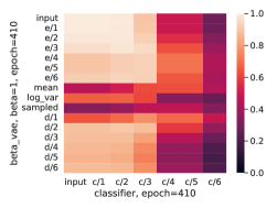
(c) Trained on SmallNorb

Figure 16: (a) shows the CKA similarity scores of activations of a classifier and a $\beta$-VAE trained on Cars3D with $\beta=1$. (b) and (c) show the CKA similarity scores of the same learning objectives and regularisation strengths but trained on dSprites and SmallNorb. All the results are averaged over 5 seeds. We can see that the representational similarity between the layers of the classifiers and of the encoder (top-left quadrant) except mean and variance is very high (CKA stays close to 1). However, the mean, variance, and sampled representations (central diagonal values) are different from the representations learned by the classifier.

Appendix I Representational similarity of VAEs at different epochs

The results obtained in Section 4.1 have shown a high similarity between the encoders at an early stage of training and fully trained. One can wonder whether these results are influenced by the choice of epochs used in Figure 2. After explaining our epoch selection process, we show below that it does not influence our results, which are consistent over snapshots taken at different stages of training.

Epoch selection

For dSprites, we took snapshots of the models at each epoch, but for Cars3D and SmallNorb, which both train for a higher number of epochs, it was not feasible computationally to calculate the CKA between every epoch. We thus saved models trained on SmallNorb every 10 epochs, and models trained on Cars3D every 25 epochs. Consequently, the epochs chosen to represent the early training stage in Section 4.1 is always the first snapshot taken for each model. Below, we preform additional experiments with a broader range of epoch numbers to show that the results are consistent with our findings in the main paper, and they do not depend on specific epochs.

Similarity changes over multiple epochs

In Figures 17, 18, and 19, we can observe the same trend of learning phases as in Section 4.1. First, the encoder is learned, as shown by the high representational similarity of the upper-left quadrant of  Figures 17(a), 18(a), and 19(a). Then, the decoder is learned, as shown by the increased representational similarity of the bottom-right quadrant of Figures 17(b), 18(b), and 19(b). Finally, further small refinements of the encoder and decoder representations take place in the remaining training time, as shown by the slight increase of representational similarity in Figures 17(c), 18(c), and 19(c), and Figures 17(d), 18(d), and 19(d).

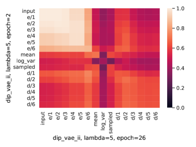
(a) Epoch 2

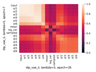
(b) Epoch 7

(c) Epoch 14

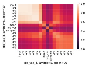
(d) Epoch 19

(e) Epoch 26

Figure 17: (a), (b), (c), (d), and (e) show the representational similarity between DIP-VAE II after full training, and at epochs 2, 7, 14, 19, and 26, respectively. All models are trained on dSprites and the results are averaged over 5 runs.

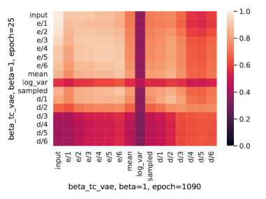
(a) Epoch 25

(b) Epoch 292

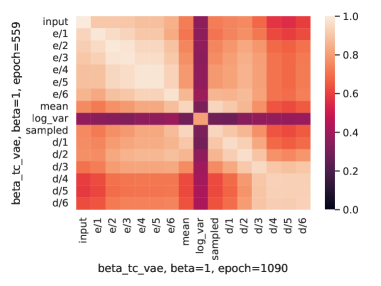
(c) Epoch 559

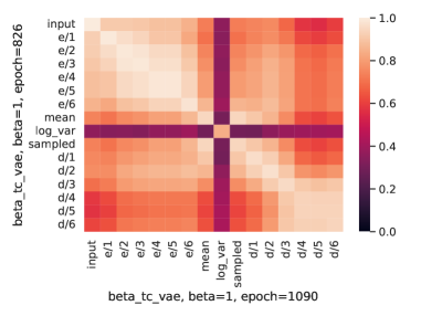
(d) Epoch 826

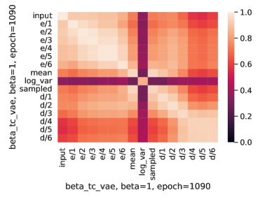
(e) Epoch 1090

Figure 18: (a), (b), (c), (d) and (e) show the representational similarity between $\beta$-TC VAE after full training, and at epochs 25, 292, 559, 826, and 1090 respectively. All models are trained on Cars3D and the results are averaged over 5 runs.

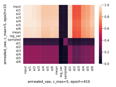
(a) Epoch 10

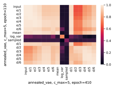
(b) Epoch 110

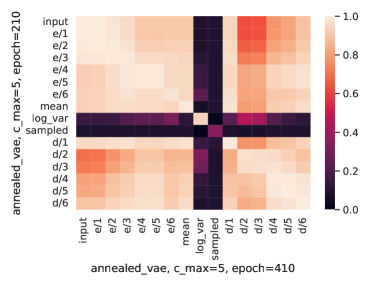
(c) Epoch 210

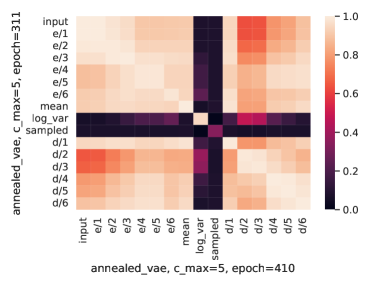
(d) Epoch 311

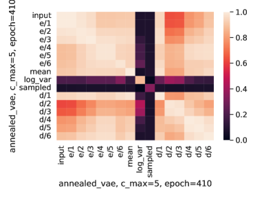
(e) Epoch 311

Figure 19: (a), (b), (c), (d) and (e) show the representational similarity between Annealed VAE after full training, and at epochs 10, 110, 210, 311, and 410 respectively. All models are trained on SmallNorb and the results are averaged over 5 runs.

Appendix J Convergence rate of different VAEs

We can see in Figure 20 that all the models converge at the same epoch, with less regularised models reaching lower losses. While annealed VAEs start converging together with the other models, they then take longer to plateau, due to the annealing process. We can see them distinctly in the upper part of Figure 20. Overall, the epochs at which the models start to converge are consistent with our choice of epoch for early training in Section 4.1.

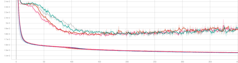
(a) Convergence on Cars3D

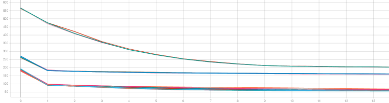
(b) Convergence on dSprites

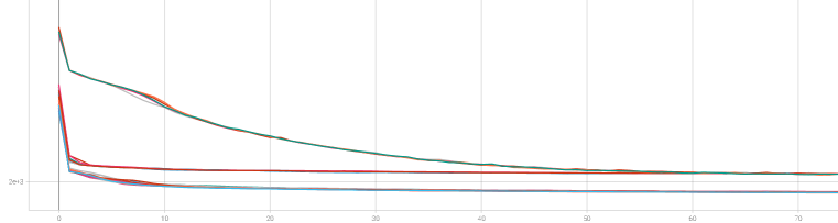
(c) Convergence on SmallNorb

Figure 20: In (a), (b), and (c), we show the model loss of each model that converged when trained on Cars3D, dSprites, and SmallNorb, respectively. For each learning objective, we display 5 runs of the least and most regularised versions.

References

- Akrami et al. (2020) Haleh Akrami, Anand A Joshi, Jian Li, Sergul Aydore, and Richard M Leahy. Brain lesion detection using a robust variational autoencoder and transfer learning. In 2020 IEEE 17th International Symposium on Biomedical Imaging (ISBI), pp. 786–790. IEEE, 2020.
- Bansal et al. (2021) Yamini Bansal, Preetum Nakkiran, and Boaz Barak. Revisiting Model Stitching to Compare Neural Representations. In Advances in Neural Information Processing Systems, 2021.
- Bonheme & Grzes (2021) Lisa Bonheme and Marek Grzes. Be More Active! Understanding the Differences between Mean and Sampled Representations of Variational Autoencoders. arXiv e-prints, 2021.
- Bonheme & Grzes (2022) Lisa Bonheme and Marek Grzes. Fondue: an algorithm to find the optimal dimensionality of the latent representations of variational autoencoders. arXiv preprint arXiv:2209.12806, 2022.
- Bowman et al. (2016) Samuel R Bowman, Luke Vilnis, Oriol Vinyals, Andrew Dai, Rafal Jozefowicz, and Samy Bengio. Generating Sentences from a Continuous Space. In Proceedings of The 20th SIGNLL Conference on Computational Natural Language Learning, 2016.
- Burgess et al. (2018) Christopher P. Burgess, Irina Higgins, Arka Pal, Loic Matthey, Nick Watters, Guillaume Desjardins, and Alexander Lerchner. Understanding Disentangling in -VAE. arXiv e-prints, 2018.
- Chen et al. (2018) Ricky T. Q. Chen, Xuechen Li, Roger B. Grosse, and David K. Duvenaud. Isolating Sources of Disentanglement in Variational Autoencoders. In Advances in Neural Information Processing Systems, volume 31, 2018.
- Cortes et al. (2012) Corinna Cortes, Mehryar Mohri, and Afshin Rostamizadeh. Algorithms for Learning Kernels Based on Centered Alignment. J. Mach. Learn. Res., 13(1), 2012.
- Cristianini et al. (2002) Nello Cristianini, John Shawe-Taylor, André Elisseeff, and Jaz S Kandola. On Kernel-Target Alignment. In Advances in Neural Information Processing Systems, volume 14. 2002.
- Csiszárik et al. (2021) Adrián Csiszárik, Péter Kőrösi-Szabó, Ákos K. Matszangosz, Gergely Papp, and Dániel Varga. Similarity and matching of neural network representations. In Advances in Neural Information Processing Systems, 2021.
- Dai & Wipf (2018) Bin Dai and David Wipf. Diagnosing and Enhancing VAE Models. In International Conference on Learning Representations, volume 6, 2018.
- Dai et al. (2020) Bin Dai, Ziyu Wang, and David Wipf. The Usual Suspects? Reassessing Blame for VAE Posterior Collapse. In Proceedings of the 37th International Conference on Machine Learning, 2020.
- Ding et al. (2021) Frances Ding, Jean-Stanislas Denain, and Jacob Steinhardt. Grounding Representation Similarity Through Statistical Testing. In Advances in Neural Information Processing Systems, 2021.
- Doersch (2016) Carl Doersch. Tutorial on Variational Autoencoders. arXiv e-prints, 2016.
- Escoufier (1973) Yves Escoufier. Le traitement des variables vectorielles. Biometrics, 29(4):751–760, 1973. ISSN 0006341X, 15410420. URL http://www.jstor.org/stable/2529140.
- Golub & Van Loan (2013) Gene H. Golub and Charles F. Van Loan. Matrix computations. The Johns Hopkins University Press, fourth edition edition, 2013. ISBN 9781421407944.
- Gretton et al. (2005) Arthur Gretton, Olivier Bousquet, Alex Smola, and Bernhard Schölkopf. Measuring Statistical Dependence with Hilbert-Schmidt Norms. In Algorithmic Learning Theory, 2005. ISBN 978-3-540-31696-1.
- He et al. (2019) Junxian He, Daniel Spokoyny, Graham Neubig, and Taylor Berg-Kirkpatrick. Lagging Inference Networks and Posterior Collapse in Variational Autoencoders. In International Conference on Learning Representations, volume 7, 2019.
- Higgins et al. (2017) Irina Higgins, Loic Matthey, Arka Pal, Christopher Burgess, Xavier Glorot, Matthew Botvinick, Mohamed Shakir, and Alexander Lerchner. -VAE: Learning Basic Visual Concepts with a Constrained Variational Framework. In International Conference on Learning Representations, volume 5, 2017.
- Hung et al. (2019) Hsiao-Tzu Hung, Chung-Yang Wang, Yi-Hsuan Yang, and Hsin-Min Wang. Improving automatic jazz melody generation by transfer learning techniques. In 2019 Asia-Pacific Signal and Information Processing Association Annual Summit and Conference (APSIPA ASC), pp. 339–346. IEEE, 2019.
- Inoue et al. (2018) Tadanobu Inoue, Subhajit Choudhury, Giovanni De Magistris, and Sakyasingha Dasgupta. Transfer learning from synthetic to real images using variational autoencoders for precise position detection. In 2018 25th IEEE International Conference on Image Processing (ICIP), pp. 2725–2729, 2018.
- Josse & Holmes (2016) Julie Josse and Susan Holmes. Measuring multivariate association and beyond. Statistics Surveys, 10(none):132 – 167, 2016. doi: 10.1214/16-SS116. URL https://doi.org/10.1214/16-SS116.
- Kingma & Welling (2014) Diederik P. Kingma and Max Welling. Auto-Encoding Variational Bayes. In International Conference on Learning Representations, volume 2, 2014.
- Kornblith et al. (2019) Simon Kornblith, Mohammad Norouzi, Honglak Lee, and Geoffrey Hinton. Similarity of Neural Network Representations Revisited. In Proceedings of the 36th International Conference on Machine Learning, volume 97 of Proceedings of Machine Learning Research, 2019.
- Kudugunta et al. (2019) Sneha Kudugunta, Ankur Bapna, Isaac Caswell, and Orhan Firat. Investigating Multilingual NMT Representations at Scale. In Proceedings of the 2019 Conference on Empirical Methods in Natural Language Processing and the 9th International Joint Conference on Natural Language Processing (EMNLP-IJCNLP), 2019.
- Kumar et al. (2018) Abhishek Kumar, Prasanna Sattigeri, and Avinash Balakrishnan. Variational Inference of Disentangled Latent Concepts from Unlabeled Observations. In International Conference on Learning Representations, volume 6, 2018.
- Lacoste et al. (2019) Alexandre Lacoste, Alexandra Luccioni, Victor Schmidt, and Thomas Dandres. Quantifying the carbon emissions of machine learning. arXiv preprint arXiv:1910.09700, 2019.
- LeCun et al. (2004) Yann LeCun, Fu Jie Huang, and Léon Bottou. Learning Methods for Generic Object Recognition with Invariance to Pose and Lighting. In Proceedings of the 2004 IEEE Computer Society Conference on Computer Vision and Pattern Recognition, 2004. CVPR 2004., volume 2, 2004.
- Lee & Jo (2021) Sungyeop Lee and Junghyo Jo. Information Flows of Diverse Autoencoders. Entropy, (7), 2021. doi: 10.3390/e23070862.
- Liu et al. (2021) Zhi-Song Liu, Wan-Chi Siu, and Li-Wen Wang. Variational autoencoder for reference based image super-resolution. In Proceedings of the IEEE/CVF Conference on Computer Vision and Pattern Recognition (CVPR) Workshops, pp. 516–525, June 2021.
- Liu et al. (2015) Ziwei Liu, Ping Luo, Xiaogang Wang, and Xiaoou Tang. Deep learning face attributes in the wild. In ICCV, 2015.
- Locatello et al. (2019) Francesco Locatello, Stefan Bauer, Mario Lucic, Gunnar Raetsch, Sylvain Gelly, Bernhard Schölkopf, and Olivier Bachem. Challenging Common Assumptions in the Unsupervised Learning of Disentangled Representations. In Proceedings of the 36th International Conference on Machine Learning, volume 97 of Proceedings of Machine Learning Research, 2019.
- Lovrić et al. (2021) Mario Lovrić, Tomislav Đuričić, Han T. N. Tran, Hussain Hussain, Emanuel Lacić, Morten A. Rasmussen, and Roman Kern. Should we embed in chemistry? a comparison of unsupervised transfer learning with pca, umap, and vae on molecular fingerprints. Pharmaceuticals, 14(8), 2021. ISSN 1424-8247.
- Lucas et al. (2019a) James Lucas, George Tucker, Roger B. Grosse, and Mohammad Norouzi. Understanding Posterior Collapse in Generative Latent Variable Models. In Deep Generative Models for Highly Structured Data, ICLR 2019 Workshop, 2019a.
- Lucas et al. (2019b) James Lucas, George Tucker, Roger B. Grosse, and Mohammad Norouzi. Don’t Blame the ELBO! A linear VAE Perspective on Posterior Collapse. In Advances in Neural Information Processing Systems, volume 32, 2019b.