Data Mining of Telematics Data:
Unveiling the Hidden Patterns in Driving Behaviour

Abstract

With the advancement in technology, telematics data which capture vehicle movements information are becoming available to more insurers. As these data capture the actual driving behaviour, they are expected to improve our understanding of driving risk and facilitate more accurate auto-insurance ratemaking. In this paper, we analyze an auto-insurance dataset with telematics data collected from a major European insurer. Through a detailed discussion of the telematics data structure and related data quality issues, we elaborate on practical challenges in processing and incorporating telematics information in loss modelling and ratemaking. Then, with an exploratory data analysis, we demonstrate the existence of heterogeneity in individual driving behaviour, even within the groups of policyholders with and without claims, which supports the study of telematics data. Our regression analysis reiterates the importance of telematics data in claims modelling; in particular, we propose a speed transition matrix that describes discretely recorded speed time series and produces statistically significant predictors for claim counts. We conclude that large speed transitions, together with higher maximum speed attained, nighttime driving and increased harsh braking, are associated with increased claim counts. Moreover, we empirically illustrate the learning effects in driving behaviour: we show that both severe harsh events detected at a high threshold and expected claim counts are not directly proportional with driving time or distance, but they increase at a decreasing rate.

Keywords Usage-based Insurance, Vehicle Telematics, Data Mining, Feature Engineering, Principal Component Analysis

1 Introduction

In classical auto-insurance ratemaking, insurers collect information on both the driver and the vehicle, such as driver’s age, years since driver’s licence obtained, vehicle brand and engine power, etc. Actuaries then use these features (also known as covariates) for risk classification, prediction of claim counts and loss amounts, and determination of a premium that will be sufficient to cover future claims. To facilitate subsequent discussion, these features will be described as ‘traditional’. With the advancement in technology, vehicle movements can be monitored and recorded by on-board diagnostics installed in the vehicle or on the driver’s smartphone. Such information, including global positioning system (GPS) locations, driving speed and acceleration, etc., is referred to as (vehicle) telematics data and is becoming available to more insurers (Eling and Kraft, (2020)). As these data capture the actual driving behaviour, they are expected to provide additional information on a driver’s risk that has not been captured by traditional covariates. Thus, the inclusion of telematics data should improve our understanding of driving risk and facilitate a more accurate auto-insurance ratemaking.

However, there are two major challenges. The first challenge is what information from telematics data is useful and what features should be extracted. Feature selection is a standard problem in classical insurance ratemaking as insurers have been trying to select traditional covariates which have high predictive power for the policyholders’ risk levels, but this problem becomes more complicated as telematics data are recorded very frequently, ranging from minutes (as in this work) to even seconds (as in Ma et al., (2018) and Gao et al., (2019)). Data aggregation is often employed and it usually begins at the trip level. While feature selection also depends on the specific data available to researchers, commonly considered variables include: numbers of harsh acceleration, harsh braking, cornering (with thresholds based on expert judgement), (fractions of) distances travelled in daytime/nighttime, on weekdays/weekends, on highways/ordinary roads, etc. over some duration (see Paefgen et al., (2014), Verbelen et al., (2018), Bian et al., (2018), Jin et al., (2018), Denuit et al., (2019), Ayuso et al., (2019), Huang and Meng, (2019), Sun et al., (2020), Longhi and Nanni, (2020)). Although most of these features have proven to be statistically significant predictors of accident occurrence, the use of these features can lead to loss of information. For example, any changes and trends in telematics data over time will be neglected. Recently, more researchers have started considering machine learning approaches on (raw) telematics time series, such as the use of speed-acceleration (v-a) heatmaps (Wüthrich, (2017), Gao et al., (2019), Gao et al., 2022b ), pattern recognition (Weidner et al., (2016), Weidner et al., (2017)) and prediction of time series using neural networks (Fang et al., (2021)).

The second challenge concerns how the telematics data should be incorporated in a modelling framework for insurance applications. Although telematics data are abundant, claim occurrence remains rare, which leads to an inconsistency in data granularity. In existing literature, telematics features are often aggregated at the trip level, and the yearly response (either the probability of incurring at least one claim, or the number of claims incurred) is regressed on these telematics features, leading to multiple observations for each policyholder in a year. There are three major ways of incorporating telematics information into the model. First, Baecke and Bocca, (2017), Verbelen et al., (2018), Ma et al., (2018), Jin et al., (2018), Ayuso et al., (2019), Huang and Meng, (2019), Guillen et al., (2021) and Duval et al., (2022) treat telematics features as additional covariates and these features enter into the regression model in the same way as traditional covariates. Second, Ayuso et al., (2019) and Gao et al., 2022b use telematics features as a correction to the existing, classical pricing models by performing another regression with the original estimates as offsets. Third, Denuit et al., (2019) propose a multivariate credibility framework to model telematics features jointly with claim counts, which allows a posteriori correction on the expected claim counts using the information from observed telematics data. However, a limitation often found in existing work is a mismatch between policy period and telematics observation period: researchers implicitly assume constant driving behaviour and make predictions for upcoming insurance periods based solely on observed driving history. Recently, Fang et al., (2021) have empirically shown that such approach is sub-optimal: the use of predicted telematics metrics outperforms the use of historical averages, because the latter are biased when used to describe future driving patterns.

In this paper, we analyze an auto-insurance portfolio with vehicle telematics data collected from a major European insurer, with the aim of better understanding telematics data, various patterns in individual’s driving behaviour and its relationship with claim occurrence. In general, it is challenging to handle and process telematics data, due to the massive data volume and unfamiliarity of researchers and practitioners with such data. Unlike most other existing works on telematics data, one of the focuses of this paper is on the data quality issues. We devote a section to elaborate on some of these issues and provide sample data to illustrate the situations, in the hope that our work can serve as a preface on telematics data for researchers and practitioners who are interested in utilizing telematics raw data for insurance applications. We also aim to tackle the challenge on what telematics features are useful. We first perform an exploratory data analysis: by analyzing from both a portfolio level and an individual policyholder level. We reveal why some covariates are less predictive of claim occurrence than expected. On the one hand, self-reported (traditional) covariates can be a poor risk proxy when the policyholders’ behaviour constantly deviate from what is declared, e.g. region of residence fails to proxy when the policyholder drives outside of the region or even the country. On the other hand, drivers can exhibit very different driving habits (e.g. when trips are usually made) and/or behaviour (e.g. average and maximum speed of a trip) despite the same number of reported claims, not to mention an individual’s driving habits and behaviour can also evolve over time. Then we perform a Negative Binomial regression analysis and feature selection to identify important claim predictors. In particular, we propose the use of a speed transition matrix, which can be viewed as an alternative to the v-a heatmap introduced by Wüthrich, (2017) and a solution when driving speed is discretely recorded and acceleration values are unavailable. We illustrate how the transition matrix can be used to capture and reveal different driving patterns, and discuss how the matrix can be constructed to better suit the portfolio (e.g. in accordance to the local speed limit). In the regression model, speed transition matrix supplements average and maximum driving speeds by capturing the stability in speed transitions, e.g. how often drivers harsh accelerate from 20 km/h to 80 km/h. We consider a Negative Binomial Generalized Linear Model for its interpretability and readiness for feature selection. Since the focus of this paper is on telematics feature engineering and selection, we do not consider the multivariate model proposed in Denuit et al., (2019) due to the complexity when a large number of telematics features in different formats (discrete, continuous, categorical, compositional) are included. Yet, we emphasize on the importance of using claim history and telematics data observed over the same period, which reduces bias and better relates the two without characterizing drivers in advance. Our result shows that large speed transitions, higher maximum speed attained, nighttime driving and increased harsh braking are associated with increased (expected) claim counts, which encourages further study and modelling of these features.

Our other contribution is to identify a non-directly proportional relationship between claim counts and total driving time or distance, in line with Boucher et al., (2013) and Boucher et al., (2017). While expected claim counts keep increasing as policyholders drive, we find that on average, every additional mile or hour travelled is less risky than the previous. Hence, simply linearly scaling insurance premium with mileage or total driving time will be insufficient for accurate ratemaking. More importantly, we discover a similar pattern exists between severe harsh events (i.e., those detected at a higher threshold) and total driving time or distance, where it takes increasingly longer for the next event to arrive. This may be how learning effect - the idea that as drivers spend more time on the road, they become more experienced and can react to road conditions better - is reflected in driving behaviour. While we have not found a formal definition of learning effect in the literature, motivated by empirical observations and analysis from data, we define it as the decreasing rate of severe harsh event arrivals as cumulative driving time (or distance) increases.

The remainder of this paper is organized as follows. Section 2 gives an overview of the raw telematics data, and describes some data quality issues encountered and the cleaning procedure therefore employed. Section 3 provides a detailed exploratory data analysis from both a portfolio level and an individual policyholder level and describes our feature engineering process. Then, Section 4 identifies important predictors of auto-insurance claim counts via a regression analysis, reveals a non-directly proportional relationship between (expected) claim counts and total driving time or distance, and discovers a similar relationship in severe harsh event arrivals. Finally, Section 5 concludes with some future directions on the research of telematics related to actuarial science.

2 Data Description and Challenges

This section provides a description of the raw data which we will work on throughout this paper. We will discuss the challenges faced and the cleaning procedure employed to arrive at a more complete data structure. While existing works such as Meng et al., (2022) and Gao et al., 2022a focus on missing data and the reliability of acceleration values from different sources, our discussion will address more general issues such as non-chronological records, difficulties in trip detection and unreliable trips.

2.1 Overview of Raw Data

Our auto-insurance dataset originates from a major European insurer. We have information collected from over 1,600 telematics tracking devices, with tracking period beginning as early as mid 2017 and ending as late as mid 2020. For each device, we have the following information:

1. Raw telematics records

   • Recorded at each minute are the following information: date and time, GPS coordinates, GPS speed and device status. If a harsh driving event occurs, then the aforementioned information at that particular moment will also be recorded.

   • Harsh driving events include harsh acceleration, braking, left and right cornering which are detected at 0.5G (G-force), where 1G is 9.8 m/s². In addition, stronger and more abrupt harsh events are detected at 1.5G and are recorded separately from the aforementioned events.

2. Trip lists

   • For each trip, the following are recorded: the date and time when the trip starts and ends (referred to as ‘trip start time’ and ‘trip end time’ hereafter), distance travelled, duration, road types (in proportions), average speed and maximum speed.

There are two immediate challenges at this stage of data processing. On the one hand, the data volume of raw telematics records is massive. The exact trip start time and trip end time are unclear based solely on these records, as will be discussed in Section 2.2. Moreover, since information is recorded at each minute, acceleration, average speed, distance travelled, and road type (e.g. urban road/highway) are hard or impossible to derive. On the other hand, harsh events detected during each trip are not included in the trip lists. Hence there is a need to combine the two sources to get a more complete summary of each trip.

We also have policy data which include information on both the policyholders and the vehicles. These policy records have coverage beginning as early as mid 2017, and ending as late as end of 2021. All policies are initially written for a one-year coverage, but some may have shorter coverage due to policy cancellation. Since a telematics tracking device may be reused due to policy renewal and/or policy cancellation, we have more policies than devices. Detailed discussions on the variables are given in Section 3.

2.2 Data Cleaning Procedure and Challenges

In the existing actuarial literature, datasets studied related to telematics are often much smaller (up to several thousands drivers and/or observed for a shorter period of time (ranging from weeks to a year) (Baecke and Bocca, (2017), Bian et al., (2018), Jin et al., (2018), Ma et al., (2018), Denuit et al., (2019), Gao et al., (2019), Sun et al., (2020), Gao et al., 2022b ). Despite the relatively small portfolio size, we spend a considerable amount of time on data cleaning, partially due to the massive volume of raw telematics data, and partially due to some unexpected issues in the data. While some researchers have also reported the burden of data preprocessing (Meng et al., (2022) and Gao et al., 2022a ), discussions on the challenges in handling telematics data are generally lacking. Hence we would like to devote this section to discuss the data cleaning procedure employed, with emphasis on issues encountered. We hope that this can serve as both a preview and an alert for interested researchers.

As an illustration of potential issues in raw telematics data, sample trips are shown from Tables 1 to 4. DeviceId is anonymized and GPS locations are removed for privacy concerns.

• Good sample: Table 1 is a sample without any recording issues: the previous trip ends with a ‘key off’ event; the current trip starts with a ‘key on’ event, no interruption in between, and ends with a ‘key off’ event; and the next trip also begins with a ‘key on’ event.

• Non-chronological records: Although telematics observations should be made sequentially, raw telematics data may not be recorded in chronological order in reality. As shown in Table 2, the observations between 18:58 to 19:03 enter the system at a later time. Re-ordering by date and time should be straight-forward in any programming languages, but the massive data volume can produce a computational burden.

• Invalid GPS records leading to device calibration: Occasionally there are invalid GPS records where GPS positions are off, such as those recorded as $(0,0)$. There are various reasons behind this, including weather conditions (e.g. heavy precipitation), external obstructions (e.g. mountains, tall buildings and bridges), and obstruction within the vehicle (e.g. metallic tinting). Although the telematics tracking device will calibrate itself, it still complicates the systematic identification of a trip, especially when GPS invalidity occurs at trip start. An example is shown in Table 3, where the ‘key on’ event occurs at 13:42:40 but the device calibrates shortly after.

• Uncertain start and end of a trip: While it is natural to assume a trip begins with a ‘key on’ event and ends with a ‘key off’ event, it is not necessarily true in practice. As demonstrated in Table 3, a ‘key on’ event does not accurately mark the beginning of a trip when the telematics tracking device calibrates its GPS positions before the vehicle starts moving. Similarly, a trip may end with prolonged idling instead of a ‘key off’ event, as displayed in Table 4.

Table 1: Sample of a Trip Without Recording Issues

	DeviceId	TimeStamp	GPSDirection	GPSSpeed	EventDescription
last trip	2022123	07/16/2018 11:51:48	0	0	KEY OFF
current trip	2022123	07/16/2018 11:55:28	0	2	KEY ON
	2022123	07/16/2018 11:56:28	0	2	POSITION IN TIME
	2022123	07/16/2018 11:57:28	132	50	POSITION IN TIME
	2022123	07/16/2018 11:58:28	144	60	POSITION IN TIME
	2022123	07/16/2018 11:59:28	134	16	POSITION IN TIME
	2022123	07/16/2018 12:00:28	32	21	POSITION IN TIME
	2022123	07/16/2018 12:01:28	28	39	POSITION IN TIME
	2022123	07/16/2018 12:02:28	38	35	POSITION IN TIME
	2022123	07/16/2018 12:03:28	42	29	POSITION IN TIME
	2022123	07/16/2018 12:04:28	38	11	POSITION IN TIME
	2022123	07/16/2018 12:05:28	56	14	POSITION IN TIME
	2022123	07/16/2018 12:06:28	0	4	POSITION IN TIME
	2022123	07/16/2018 12:07:28	0	3	POSITION IN TIME
	2022123	07/16/2018 12:08:28	0	1	POSITION IN TIME
	2022123	07/16/2018 12:09:28	0	2	POSITION IN TIME
	2022123	07/16/2018 12:10:28	0	2	POSITION IN TIME
	2022123	07/16/2018 12:10:45	0	1	KEY OFF
next trip	2022123	07/17/2018 13:27:16	0	1	KEY ON

Table 2: Sample of a Trip Not in Chronological Order

	DeviceId	TimeStamp	GPSDirection	GPSSpeed	EventDescription
	2022123	07/19/2018 18:56:21	296	38	POSITION IN TIME
	2022123	07/19/2018 18:57:21	276	30	POSITION IN TIME
	2022123	07/19/2018 19:04:21	254	85	POSITION IN TIME
	2022123	07/19/2018 19:05:21	258	79	POSITION IN TIME
	2022123	07/19/2018 19:06:21	258	79	POSITION IN TIME
	2022123	07/19/2018 19:07:21	254	58	POSITION IN TIME
	2022123	07/19/2018 19:08:21	236	64	POSITION IN TIME
time ordering	2022123	07/19/2018 18:58:21	270	38	POSITION IN TIME
	2022123	07/19/2018 18:59:21	246	42	POSITION IN TIME
	2022123	07/19/2018 19:00:21	246	61	POSITION IN TIME
	2022123	07/19/2018 19:01:21	246	79	POSITION IN TIME
	2022123	07/19/2018 19:02:21	236	49	POSITION IN TIME
	2022123	07/19/2018 19:03:21	252	81	POSITION IN TIME
	2022123	07/19/2018 19:09:21	272	49	POSITION IN TIME

Table 3: Sample of a Trip With Device Calibration

	DeviceId	TimeStamp	GPSDirection	GPSSpeed	EventDescription
	160	02/25/2019 13:42:40	0	0	KEY ON
device calibration	160	02/25/2019 13:42:53	0	3	FIX GPS OK
	160	02/25/2019 13:43:40	144	31	POSITION IN TIME
	160	02/25/2019 13:44:40	108	72	POSITION IN TIME
	160	02/25/2019 13:45:40	126	89	POSITION IN TIME
	160	02/25/2019 13:46:40	134	93	POSITION IN TIME
	160	02/25/2019 13:47:40	112	87	POSITION IN TIME
	160	02/25/2019 13:48:40	114	75	POSITION IN TIME
	160	02/25/2019 13:49:40	128	77	POSITION IN TIME
	160	02/25/2019 13:50:40	150	79	POSITION IN TIME
	160	02/25/2019 13:51:40	140	83	POSITION IN TIME
	160	02/25/2019 13:52:40	114	79	POSITION IN TIME

Table 4: Sample of a Trip With No ‘Key Off’ Event

	DeviceId	TimeStamp	GPSDirection	GPSSpeed	EventDescription
last trip	2022123	07/26/2018 09:36:32	170	22	POSITION IN TIME
current trip	2022123	07/26/2018 09:53:31	0	1	KEY ON
	2022123	07/26/2018 09:54:30	26	20	POSITION IN TIME
	2022123	07/26/2018 09:55:30	32	34	POSITION IN TIME
	2022123	07/26/2018 09:56:30	122	13	POSITION IN TIME
	2022123	07/26/2018 09:57:30	0	1	POSITION IN TIME
	2022123	07/26/2018 09:58:30	0	1	POSITION IN TIME
	2022123	07/26/2018 09:59:30	0	1	POSITION IN TIME
	2022123	07/26/2018 09:59:56	0	1	KEY OFF

Detected trips do not necessarily match the trip lists in Section 2.1 due to the last issue above, hence we begin with the trip list of each device instead. For each device and for each trip on its list, we find the indices corresponding to the start and end of each trip in the raw telematics data, and summarize the numbers of detected harsh events and the maximum speed in between. Ideally, we should be able to find the exact time-points of both the start and end; however, this can occasionally fail due to unforeseen reasons such as system error and delay, and the time-points from both sources can differ from a second to several days. Hence, we search for the timestamp with the minimal absolute time difference.

Remark: We do recognize the fact that the trip lists which contain duration, distance, etc. do not come without effort - either the insurer which provided us the data have additional information from the telematics tracking device and/or the drivers, or they have put in effort to produce the lists. In fact, how to reasonably identify a trip, such that it is neither terminated if the vehicle just stops for a while (e.g. to buy gas), nor it goes on forever even if the vehicle has already parked but a ‘key off’ event is not registered, is a practical problem faced by the telematics industry. Possible solutions include filtering for invalid GPS points and manually defining a threshold for idling time, say three minutes.

For each device, we now have a list of trips with information including start and end date and time, distance travelled, duration, average and maximum speed, road types travelled (in proportions), and the numbers of detected harsh events. However there are still some problematic observations, e.g. trips lasting only 3 seconds, with average speed of 1,560 km/h, and maximum speed of 0 km/h, etc. To improve data quality for reasonable analysis, we filter the trips using the following criteria: duration of at least 3 minutes, average speed between 5 and 150 km/h, maximum speed of at least 10 km/h, and time differences between two sources within a minute. We expect the filtered trips to be able to show at least some driving behaviour.

For each policy, we then extract the trips that are within the insurance coverage period, with attention paid on whether the policy is cancelled early. We summarize the following on a policy level: start date of the first and last recorded trips, total number of trips, driving time and distance, numbers of detected harsh events, time-weighted mean of average speed from each trip and maximum speed attained. Although some literatures have suggested that three months of telematics data are sufficient to attain stable characterization of driving behaviour (Baecke and Bocca, (2017) and Duval et al., (2022)), they implicitly assume that driving behaviour is constant over the time period. In contrast, we filter policies such that the total deviation between telematics observation and insurance coverage periods is no more than three months, as to ensure not to miss a considerable amount of characterization information. This leaves us with 1,458 policies and a total of 1.83 million trips.

3 Exploratory Data Analysis and Feature Engineering

This section provides an exploratory data analysis and outlines the feature engineering process employed. We also demonstrate the heterogeneity in policyholders’ driving behaviour through an analysis of telematics data, from both a portfolio level and an individual policy level.

3.1 Description of Cleaned Data

The cleaned dataset has 1,458 policies from 1,073 unique policyholders. Among these policyholders, 717 (66.8%), 327 (30.5%) and 29 (2.7%) are observed for 1, 2 and 3 insurance periods (mostly one year, but can be shorter due to policy cancellation). 44 (3%), 395 (27.1%), 969 (66.5%) and 50 (3.4%) policies begin in years 2017, 2018, 2019 and 2020 respectively. Table LABEL:table:_covariates-traditional shows the claim counts and a list of traditional covariates, which are information on the policy, the policyholder and the vehicle; whilst Table LABEL:table:_covariates-telematics shows a list of covariates derived from telematics data. Table LABEL:table:_summary-stats provides the summary statistics of numerical variables in the two tables.

There are limitations in some of the covariates, imposing the need of excluding them. First, we see that age has 37% non-numerical/missing values. The reason is that these policies are written under a company entity and hence the policyholder’s age is unknown. Based solely on policyholders whose age data are available, we do not see a significant difference in policyholder’s age with and without claims: the medians are 40.00 and 42.00, while the means are 42.44 and 43.86 respectively. The mean claim rate in this group is 0.4651, which is close to the portfolio mean of 0.4465. It is worth mentioning that while some telematics datasets studied in actuarial science have focused on younger policyholders and hence an arguably more homogeneous group (Boucher et al., (2017), Ayuso et al., (2019), Denuit et al., (2019), Henckaerts and Antonio, (2022)), there is not such indication in our dataset. Second, engine_cc, engine_power and mileage have unreliable minimum values. While a zero engine capacity is clearly questionable, the usual range of engine power is above 100 horsepower, which is equivalent to 74 kilowatts. Moreover, a zero mileage is also untrustable which suggests the need of mileage records from telematics instead of self-reported. Finally, categorical variables such as county and make have many levels, while the latter may also have duplicates due to an unstandardized list of vehicle brands, hence we will exclude them and replace with other variables.

From a modelling perspective, we will further exclude the following: first, avg_distance and avg_time as to not average out trip characteristics beforehand; second, num_trips due to the correlation between total_distance or total_time and avg_speed; and finally, prop_other_road since it is compositional with prop_urban, prop_extra_urban and prop_highway (i.e., they sum to 100), and values of prop_other_road are relatively small (as reflected by the interquartile range at lower values), hence we will consider only the other three roadtypes. For convenience, these proportions will be considered together and referred to as prop_roadtype hereafter.

While most of the telematics covariates are extracted and/or summarized directly from the cleaned data in Section 2, we introduce in Section 3.2 two additional sets of variables: principal components (PCs) of speed transition matrix and proportions of driving in different times of the day.

3.2 Feature Engineering on Telematics Data and the Speed Transition Matrix

First, we aim to extract more information from GPS speed, especially the time series structure in speed, as to supplement avg_speed and max_speed. Our data structure does not permit the use of the v-a heatmap proposed by Wüthrich, (2017): we neither have acceleration data nor able to compute acceleration values because speed is recorded per minute in the raw GPS data, while acceleration is usually measured as the change in speed per second, hence it is impossible for us to produce the same v-a heatmap. Although the unavailability of per-second speed data may seem to be a limitation that exists only in our dataset, this is actually common in practice to reduce the burden of data transmission and storage. Hence it is necessary to build general frameworks to process, analyze and model telematics data, such as speed, within the constraints of data availability (e.g. only minute-level data).

We produce instead a speed transition matrix for each policy, where each element is the empirical probability of changing from one speed bin to another. The bins are: [0, 0.5), [0.5, 10), [10, 20), [20, 30), …, [120, 130), [130, Inf). In particular, the first bin aims to capture the stationary state, the last bin is chosen according to the speed limit in the country where policies are written, and the intermediate bins are chosen to strike a balance between information granularity and dimensionality. While we have chosen a constant bin width of 10 km/h based on expert judgement, we discuss in Section 4.4 what bin width is suitable for the data, and show that the predictive power of the proposed matrix is in fact fairly robust to different bin widths. Pyrkov et al., (2018) implement a similar transition matrix approach to describe human’s locomotor activity.

For each policy, we consider the entire driving period (i.e. all trips). For example to calculate the (empirical) probability of changing from [0, 0.5) to [10, 20), we count the number of times the vehicle begins stationary and ends up between 10 to 20 km/h at the next minute, and then divide that number by the total number of times the vehicle is at rest. This construction can also be a difference between our speed transition matrix and the v-a heatmap, as our matrix considers all speeds while the latter is often truncated, e.g. Gao et al., (2019) only consider [5, 20] km/h and Gao et al., 2022b consider (0, 80] km/h. As will be shown in Section 3.4, the proposed transition matrix is able to capture a variety of patterns in individual driving behaviour. In order to include this 15-by-15 matrix in regression models, we employ principal component analysis (PCA) to produce PCs that can be used as covariates. To limit the number of covariates, as well as to see whether the PCs will actually supplement or substitute the commonly considered telematics features avg_speed and max_speed, we include only the first two PCs in our subsequent analysis. While the use of PCA will unavoidably reduce the interpretability of the original features, we attempt to understand the general patterns captured by the two PCs. Figure 1(d) visualizes the loadings of pc1 and pc2 via a heatmap, with yellow representing large, positive weights and dark blue representing small, negative weights. As expected, the two PCs focus on different areas of the speed transition matrix: pc1 emphasizes on accelerations, giving larger weights to the upper triangle, which are transitions to the higher speed bins; whilst pc2 prioritizes decelerations and stationarity, giving larger weights to the few transitions from moderate speed bins to lower speed bins, and negative weights along the diagonal, which are the few transitions within the moderate speed bins. We also provide the first two PC’s loadings from a matrix with fewer speed bins (doubled the bin width) in Figure 2(b), which demonstrate that the patterns captured are consistent.

We also consider information on when the policyholder usually drives. On the one hand, this is motivated by previous works that include this information and reveal its relevance to riskiness, such as driving during rush hours and/or at nighttime is more dangerous (Jin et al., (2018), Ayuso et al., (2019), Duval et al., (2022)). On the other hand, we do observe from our data some differences in driving behaviour at different time of the day, as shown in Table 8. After allocating driving time of each trip to the different hours, we aggregate all trips for each policy and arrive at proportions of driving in each of the 24 hours. To reduce the number of dimensions, we consider timeslots consisting of four hours each: midnight to 3:59 a.m., 4 to 7:59 a.m., 8 to 11:59 a.m., noon to 3:59 p.m., 4 to 7:59 p.m., and 8 to 11:59 p.m. Since the proportions of driving in different timeslots are again compositional with one another, we exclude the last group prop_20_24 without loss of generality. For convenience, all these proportions will be considered together and referred to as prop_time in subsequent discussion.

3.3 Portfolio Level Distribution

We first examine the GPS locations to understand the areas travelled by the drivers. While all policies are written in a single country (referred to as the ‘home country’ hereafter), trips are made all over Europe, thanks to the ease of travel granted by the European Union. We report in Tables 5 and 6 the numbers of GPS observations and harsh events in the six most frequently travelled countries (anonymized for privacy issue), for policies with and without claims respectively. We see that 6.6% and 9.4% of the GPS records from the two groups (hence 8.5% from the whole portfolio) are made outside of the home country. This may be one of the reasons why the region of residence (within the home country) reported by the policyholders has a relatively low predictive power of claim counts/riskiness, as will be shown in Section 4.

Table 5: Countries with the Most GPS Observations - Policies with Claims

	Country	Total GPS Observations	Harsh Events	Travel Frequency (%)	Harsh Event Rate (%)
1	Home country	10,837,451	101,601	93.43	0.94
2	Country A	131,162	113	1.13	0.09
3	Country B	121,394	137	1.05	0.11
4	Country C	102,041	241	0.88	0.24
5	Country D	99,243	170	0.86	0.17
6	Country E	97,821	200	0.84	0.20
	…			0.39

Table 6: Countries with the Most GPS Observations - Policies without Claims

	Country	Total GPS Observations	Harsh Events	Travel Frequency (%)	Harsh Event Rate (%)
1	Home country	23,427,201	155,597	90.60	0.66
2	Country A	756,033	248	2.92	0.03
3	Country B	330,149	318	1.28	0.10
4	Country C	254,300	846	0.98	0.33
5	Country D	213,322	620	0.82	0.29
6	Country E	181,073	175	0.70	0.10
	…			0.47

Table 7: Two-Sample Means and Medians of Selected Covariates. Last column reports the p-value for testing the null hypothesis that the two means are equal.

	claimed		no claim		p-value
	mean	median	mean	median
car_value	169423.4	138355.8	157029.5	134202.3	0.064	.
vehicle_age	2.2	1.0	2.3	1.0	0.402
max_weight	2149.9	2040.0	2161.2	2030.0	0.668
policy_period	1.0	1.0	0.9	1.0	0.000	***
total_distance	16370.2	13122.8	14040.0	10554.2	0.002	*
total_time	26552.8	23091.6	21961.7	18850.8	0.000	***
avg_speed	36.1	34.8	36.3	35.2	0.747
max_speed	168.0	166.0	157.7	155.0	0.000	***
num_acc	101.3	24.0	54.8	9.0	0.001	**
num_brake	67.2	43.0	42.8	28.0	0.000	***
num_left	55.6	11.0	28.8	7.0	0.003	**
num_right	34.4	8.0	19.9	5.0	0.015	*
num_severe	3.4	1.0	2.9	1.0	0.398
num_trips	1489.4	1330.0	1163.6	1076.0	0.000	***
pc1	0.13	-0.67	-0.05	-1.10	0.578
pc2	0.83	0.56	-0.32	-0.43	0.000	***

• Significance codes: 0 ‘***’, 0.001 ‘**’, 0.01 ‘*’, 0.05 ‘.’, 0.1 ‘ ’, 1

Classifying policies into ‘claimed’ and ‘no claim’ groups, in Table 7 we report the two-sample means and medians of selected covariates, where the last column indicates whether the null hypothesis that the two means are equal can be rejected at a significance level of 5%. Then in Figures 1(d) and 3(f) we show grouped histograms of the telematics covariates having significantly different means, while in Figure 4(b) we show grouped boxplots of compositional covariates. As mentioned, pc1 gives positive weights to the transitions towards higher speed bins, whilst pc2 gives positive weights to the few transitions from moderate speed bins to lower speed bins, and negative weights along the diagonal, which are the few transitions within the moderate speed bins. Hence large speed transitions will be represented by larger, positive values of pc1 andpc2. As displayed in the grouped histograms in Figure 1(d), the group with claims has higher PC1 and PC2 on average, when compared to the group without claim, and the difference is more obvious in PC2. This suggests that the two groups differ more in deceleration patterns than in acceleration patterns. In Figure 3(f) we observe that the group with claims is driving longer on average, in terms of both distance and time, and is making more harsh accelerations and braking, with the difference in the latter being more distinct; this aligns with the interpretations from the PC’s. The maximum speed attained is also generally higher. The proportions driven in different roadtypes and timeslots are generally close between the two groups. Overall, the group with claims is driving slightly less in urban zones but more on highways, as well as more between 8 p.m. to midnight.

Figure 1: First Two Principal Components (PCs) of Speed Transition Matrix. First Row: Loadings, Second Row: Grouped Histogram of Resulted PCs - Red: With Claims, Blue: Without Claim.

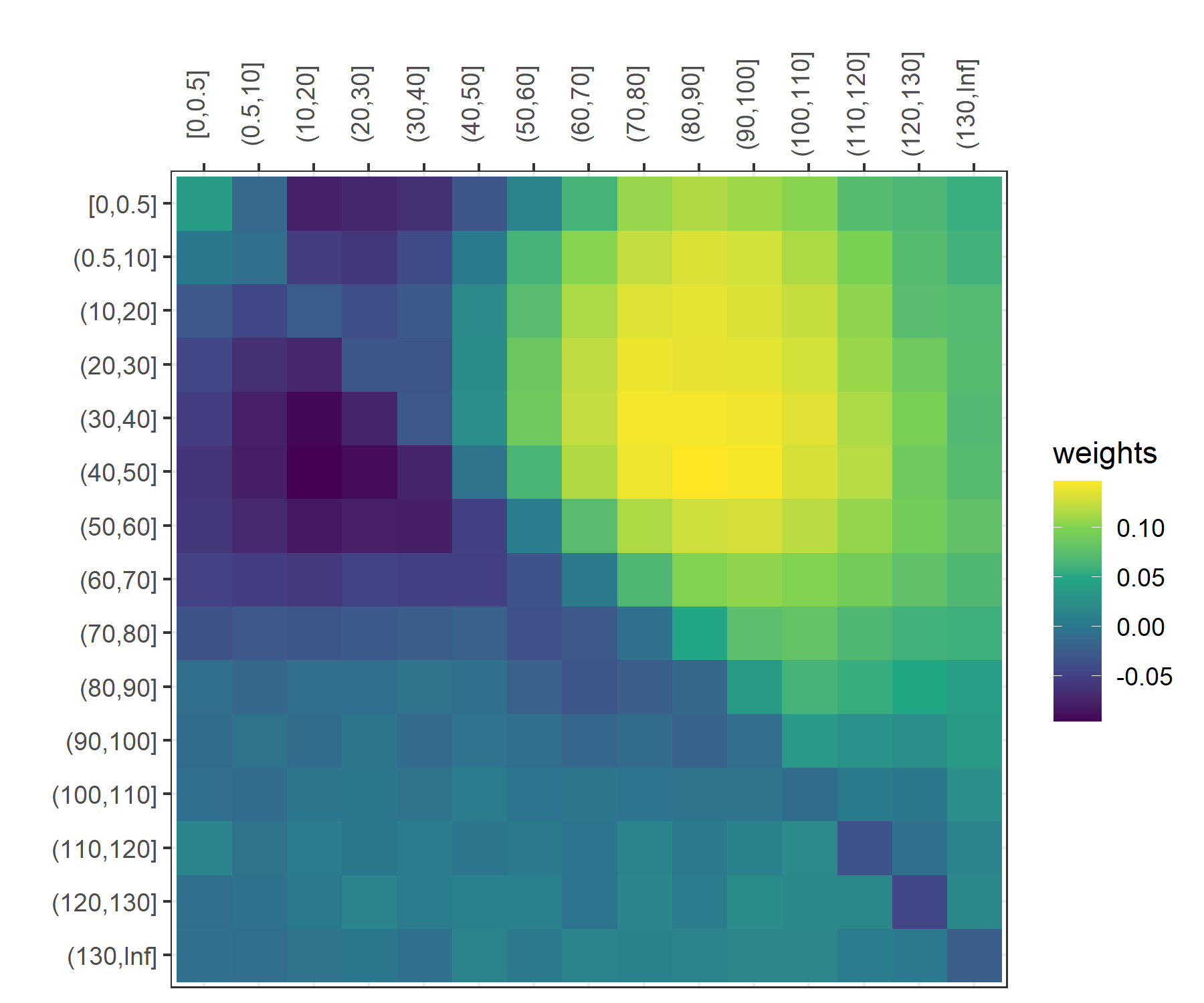
(a) Loadings of PC1

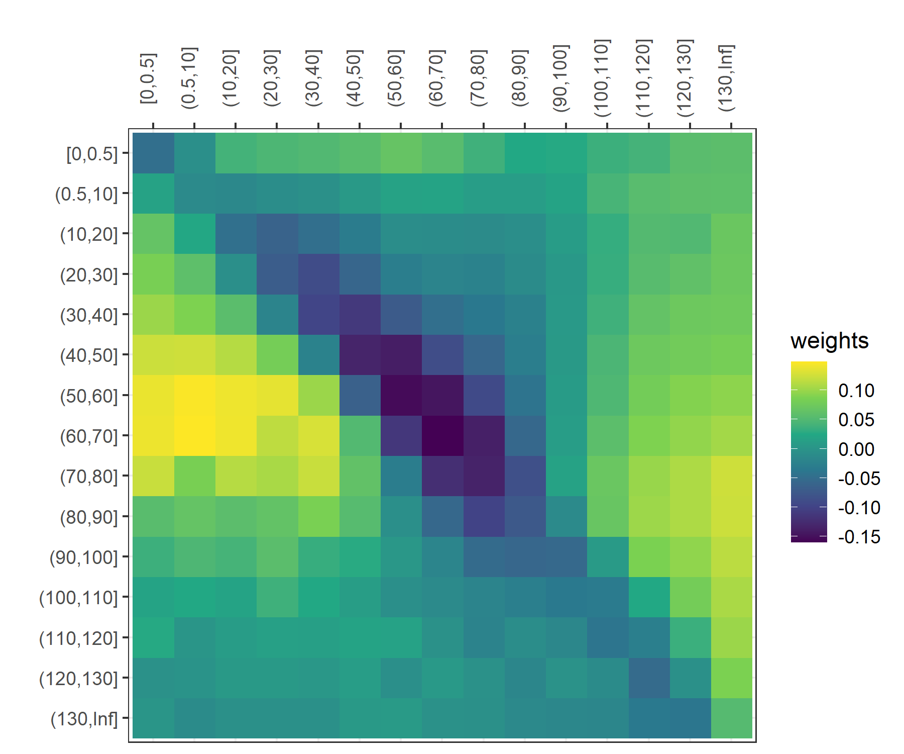
(b) Loadings of PC2

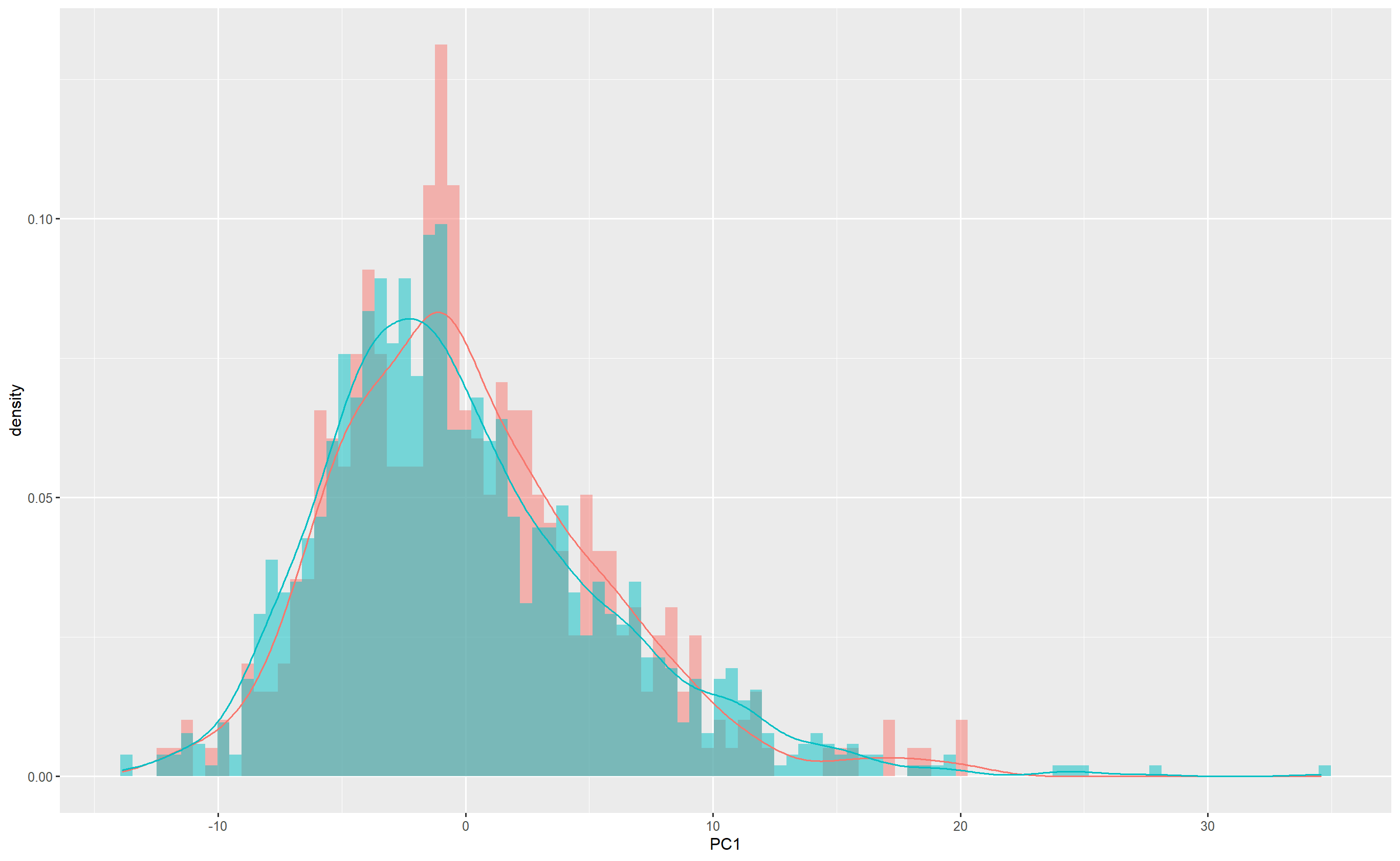
(c) PC1 of Speed Transition Matrix

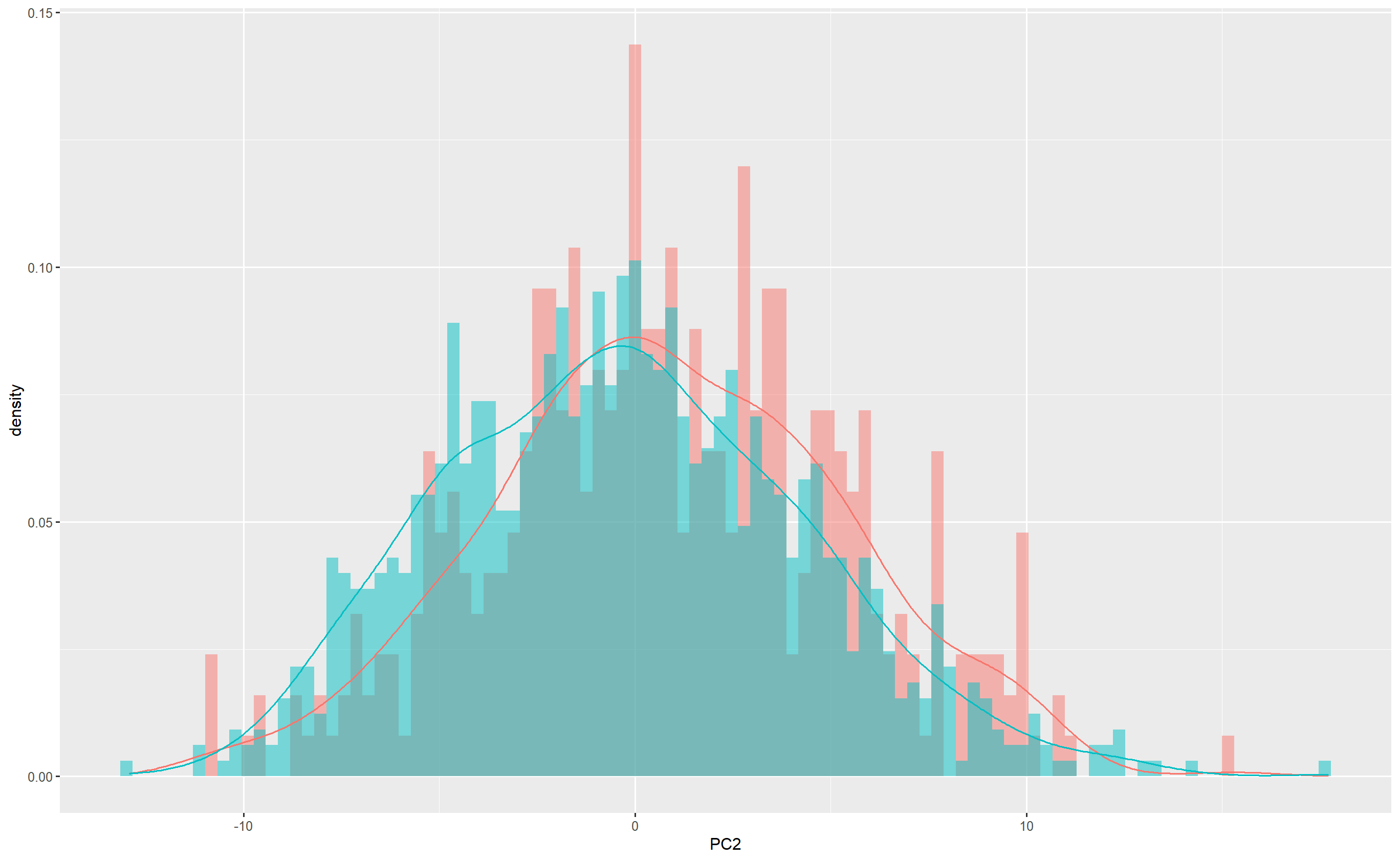
(d) PC2 of Speed Transition Matrix

Figure 2: First Two Principal Components (PCs) of Speed Transition Matrix with Fewer Speed Bins. Patterns are consistent with the matrix with more speed bins and used for the regression analysis.

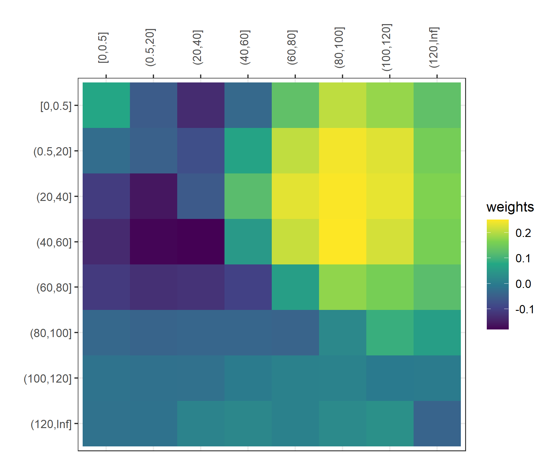
(a) Loadings of PC1

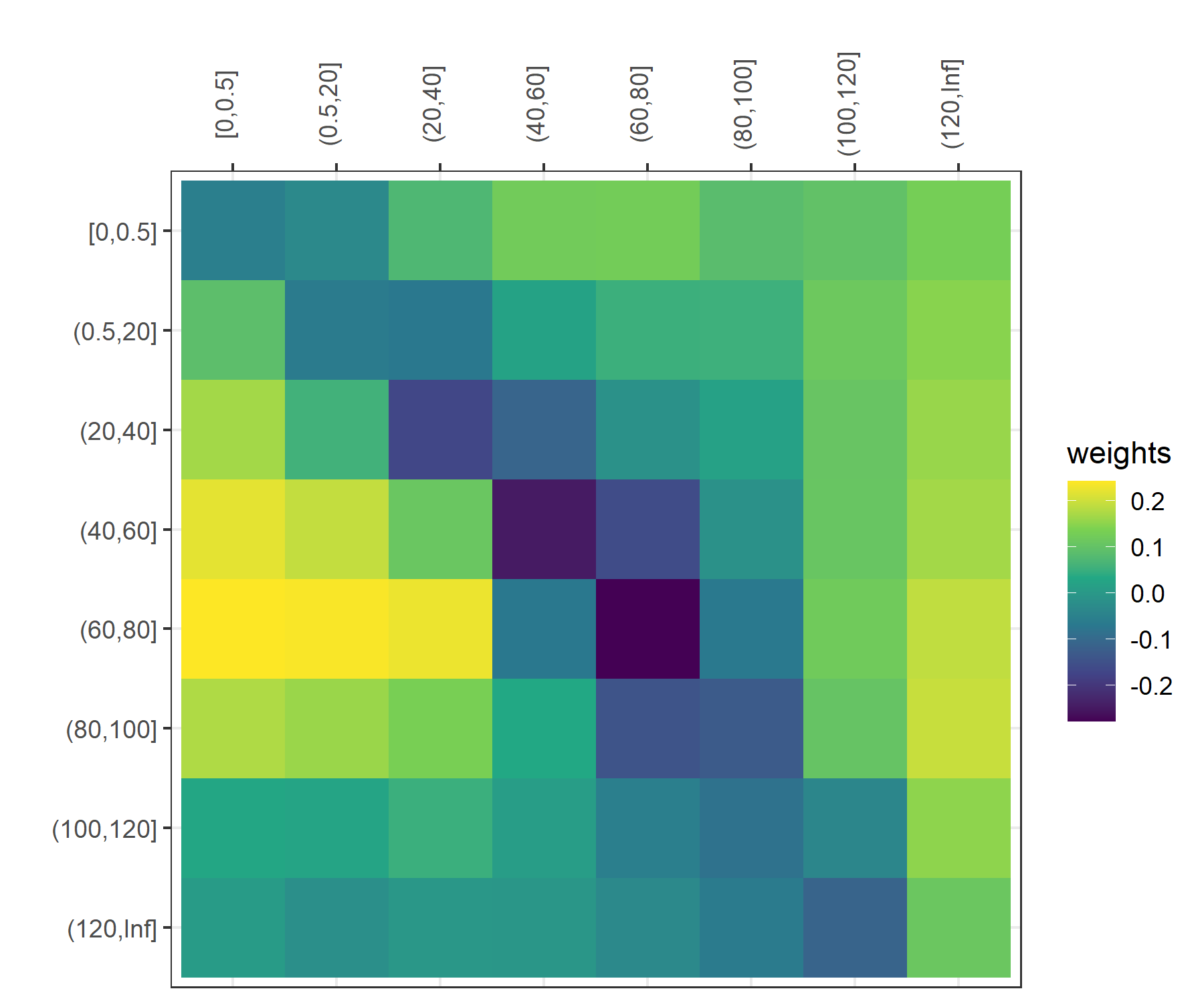
(b) Loadings of PC2

Figure 3: Grouped Histograms of Selected Telematics Features. Red: With Claims, Blue: Without Claim.

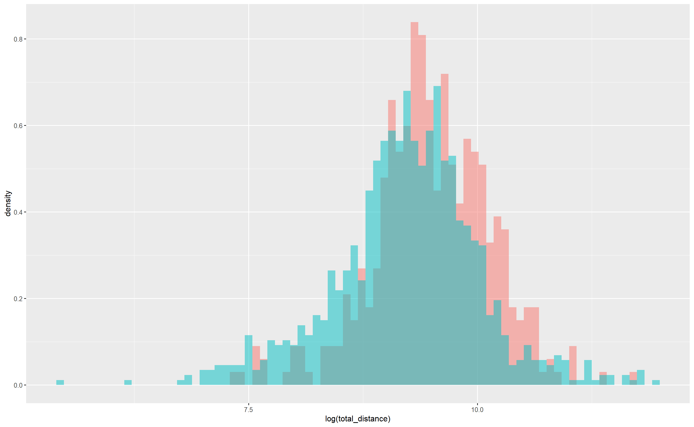
(a) Logged Total Distance

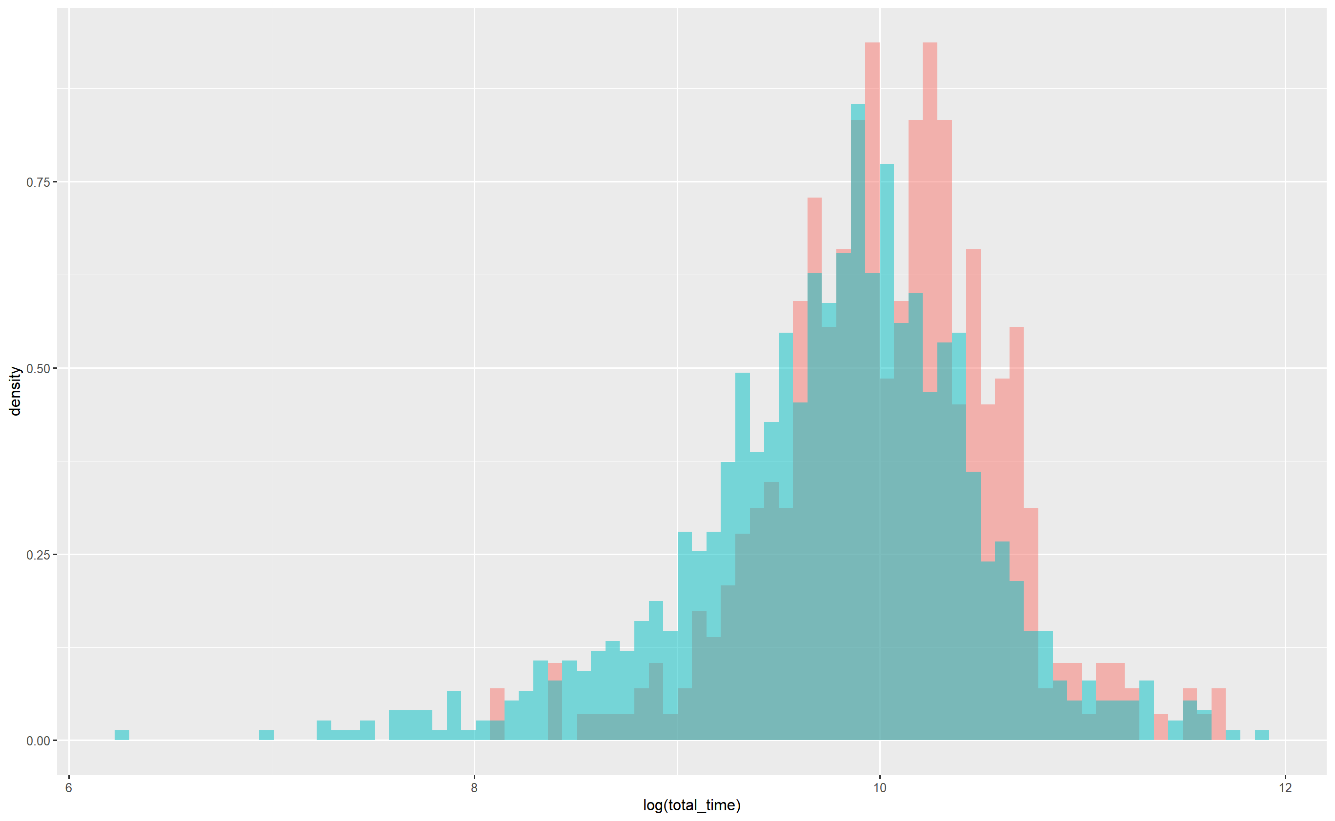
(b) Logged Total Time

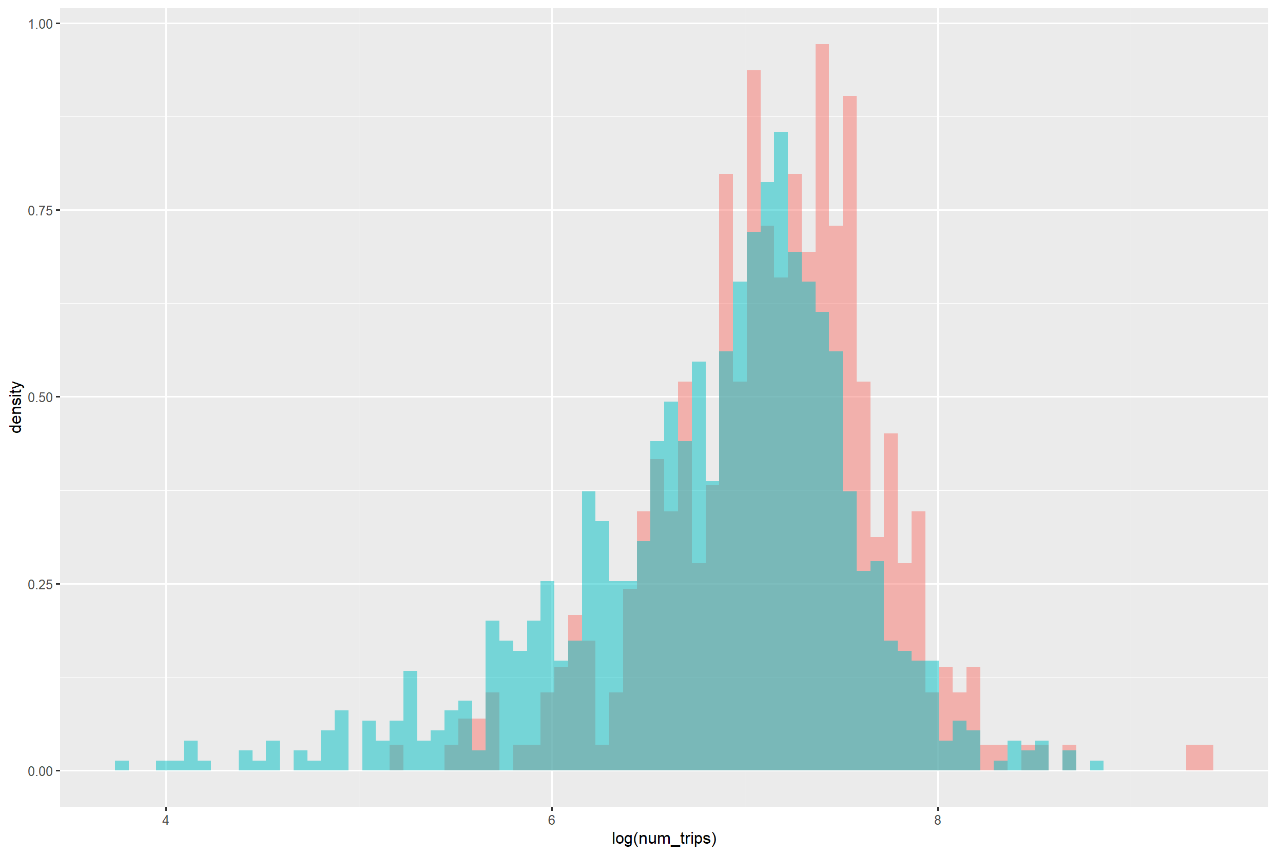
(c) Logged Number of Trips

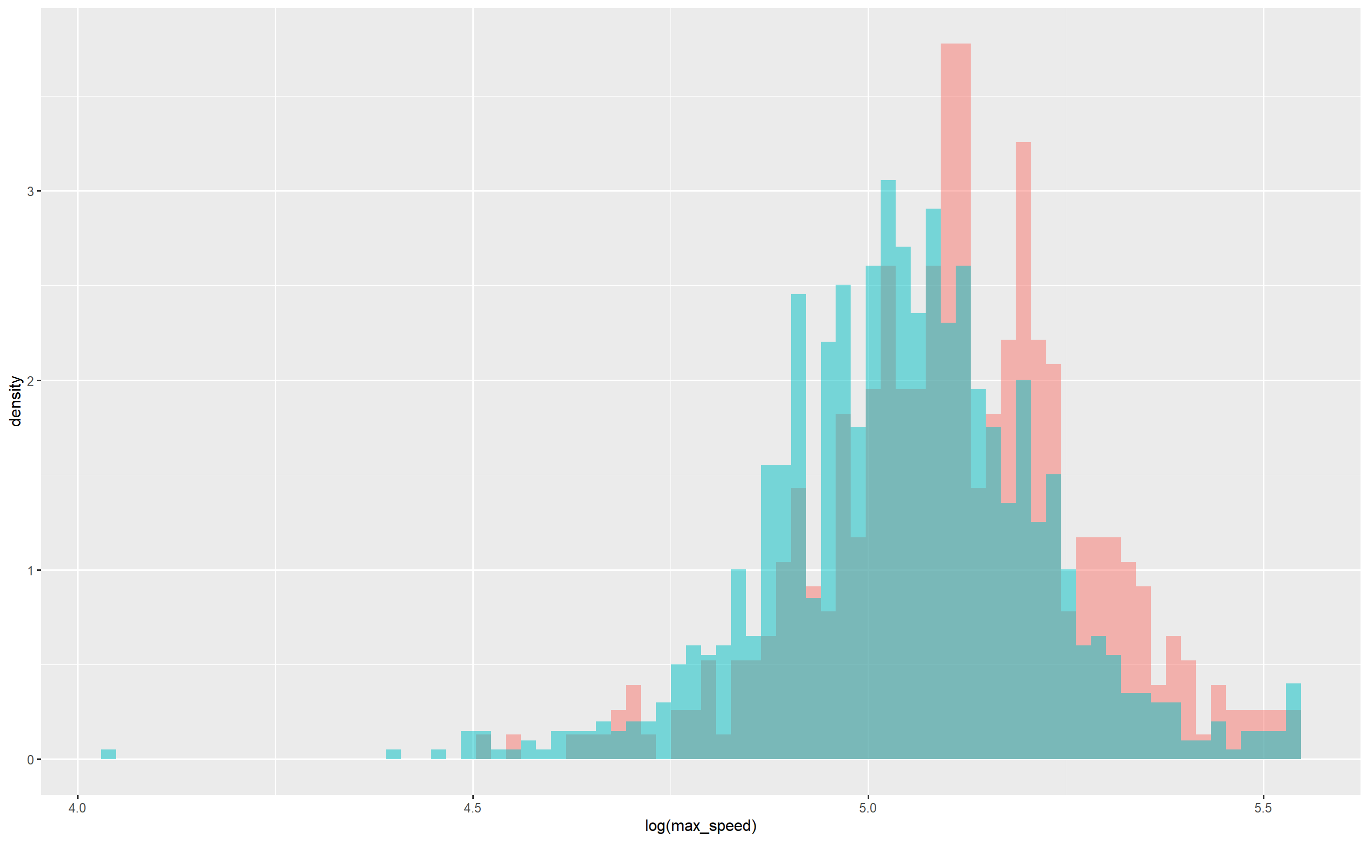
(d) Logged Max Speed

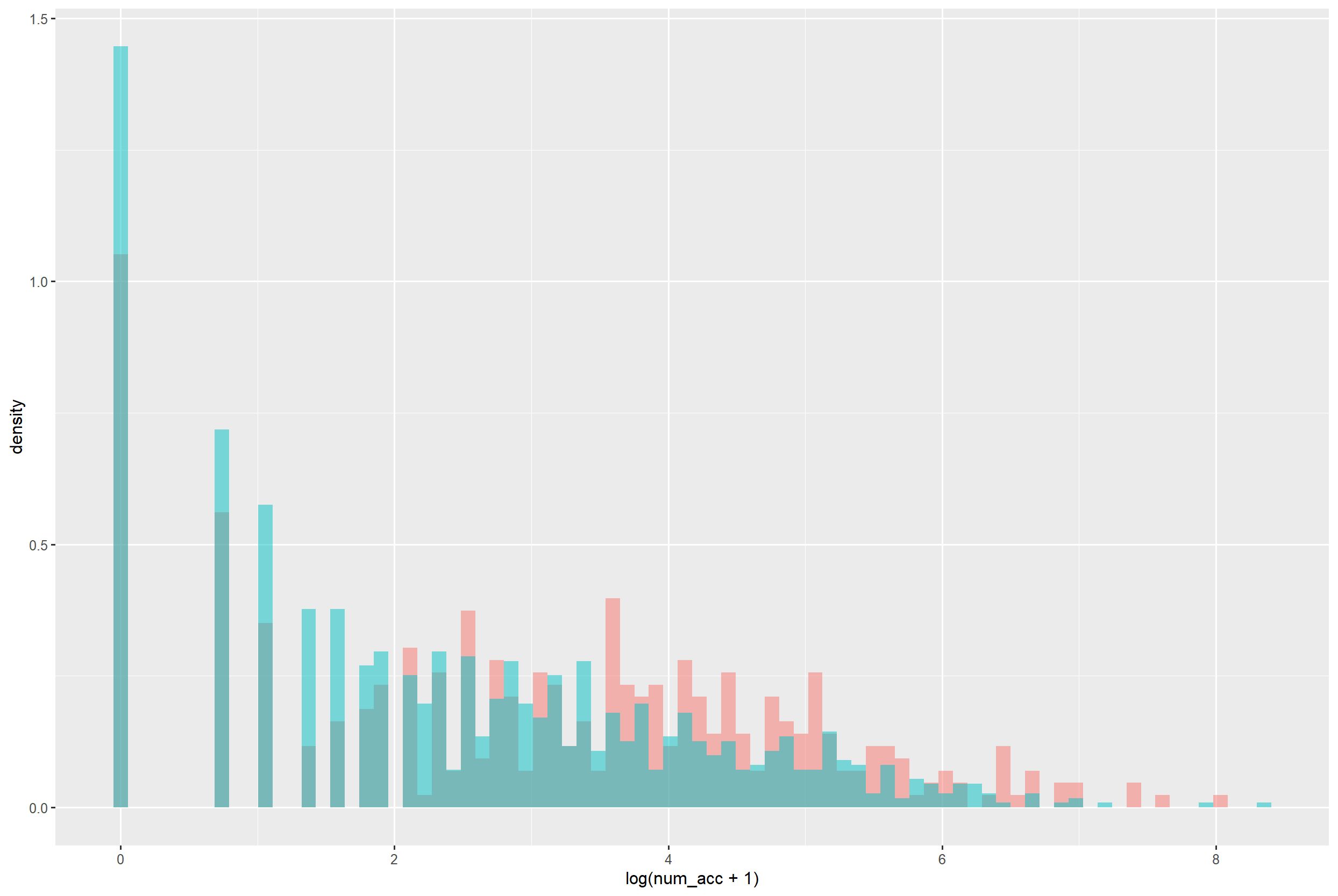
(e) Logged Number of Harsh Accelerations

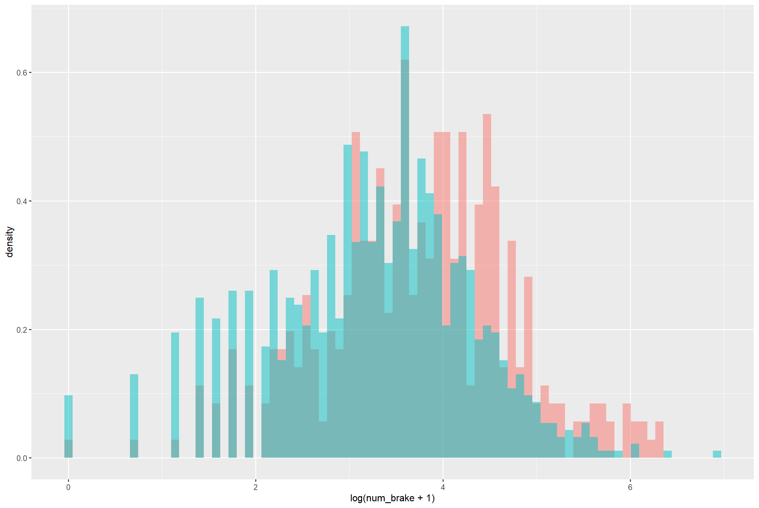
(f) Logged Number of Harsh Braking

Figure 4: Grouped Boxplots of Compositional Covariates. Red: With Claims, Blue: Without Claims.

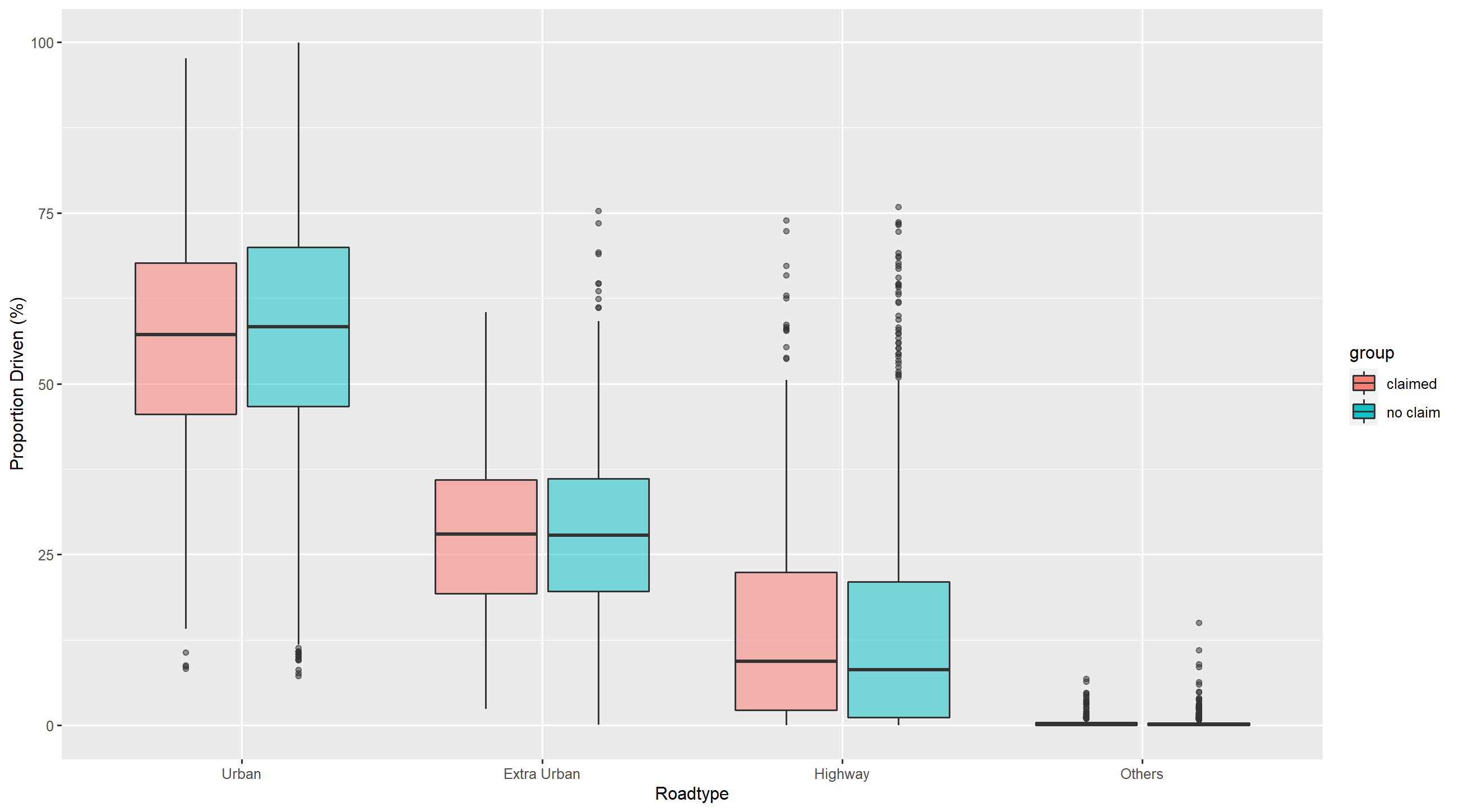
(a) Proportion Driven on Different Roadtypes

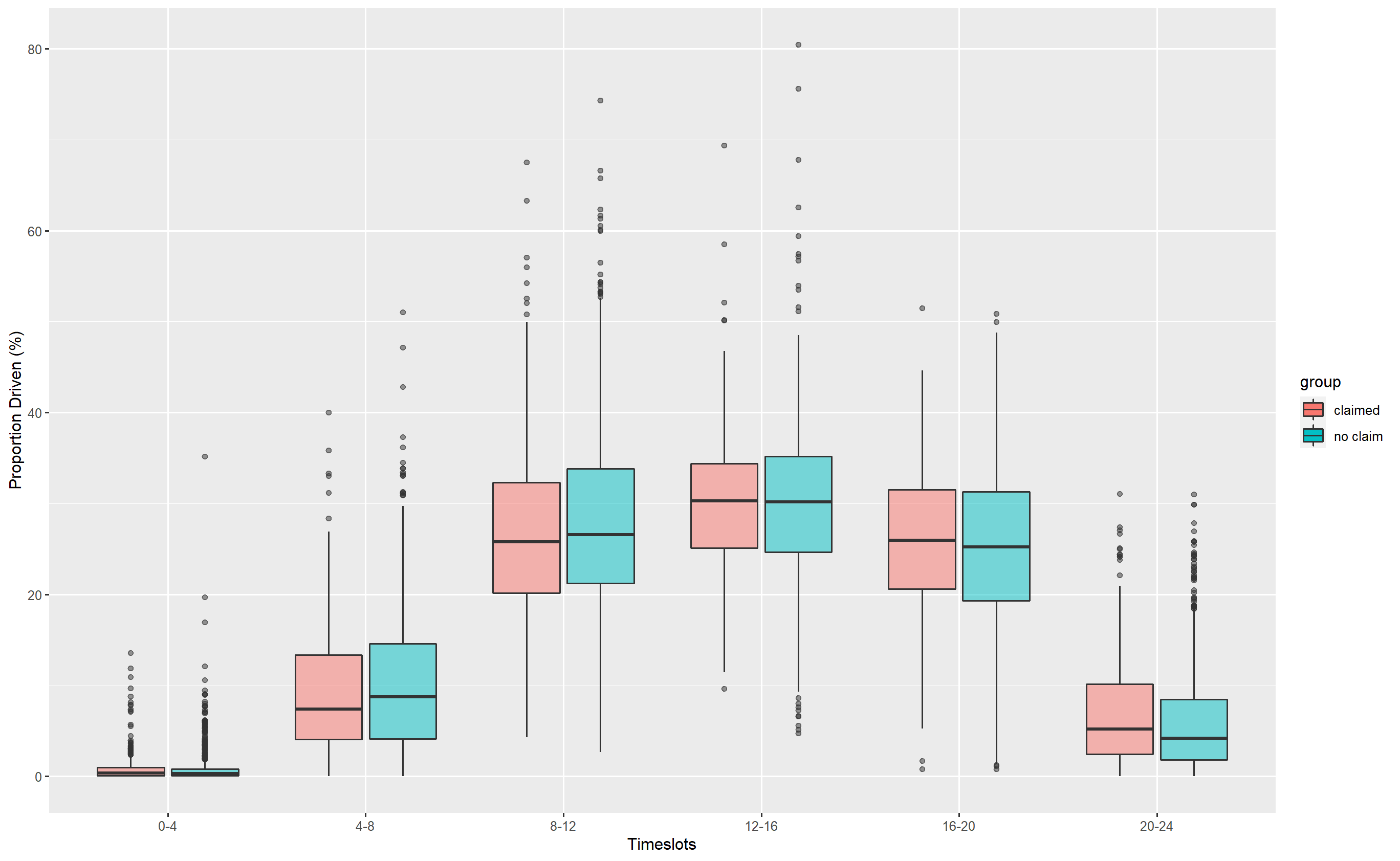
(b) Proportion Driven in Different Timeslots

3.4 Individual Heterogeneity

In this section we explore briefly the driving behaviour of individual drivers, through their driving speed and start time of each trip.

The time when drivers begin their trips dominates the different timeslots when they are driving, and both are related to differences in driving behaviour. In Table 8 we report the two-sample means of maximum speed and harsh event rate (i.e., per minute) in different timeslots. For simplicity, we categorize trips mainly according to their start time, e.g. a trip is categorized in the first group if it begins between midnight to 2 a.m., or begins between 3 a.m. to 4 a.m. and ends before 4:15 a.m. We observe that maximum speed and harsh event rate are generally higher during nighttime, and they are highest between midnight to 4 a.m., followed by 8 p.m. to midnight. Yet, we cannot conclude that driving between midnight to 4 a.m. is the most dangerous since the number of trips begun in this timeslot is the lowest.

Figures 5(b) and 6(b) show the trip-based mean and maximum speeds, respectively, for policies with and without claims. Each line represents a policy’s empirical density of mean/maximum speed per trip. We apply a simple clustering of whether the density’s mode is within (blue) or beyond (red) the 95% confidence interval of the group. We observe quite a heterogeneity in driving behaviour, evidenced by first the multimodality in individual empirical density, and second the various density shapes even among the policies that have or have not filed claims.

While the heterogeneity within each group may average out and lead to some difference between the two groups on an aggregate level as in Figure 3(f), the predictive power (for claim occurrence) of some of the telematics covariates may be undermined. As will be shown in Section 4, common summary statistics of speed, such as average and maximum, have reduced predictive power especially when summarized across the entire policy period (i.e. over multiple trips). This suggests the need of a more flexible feature engineering and extraction for telematics data if we would like to make full use of them for auto-insurance ratemaking. For example, the proposed speed transition matrix takes into account all trips, all speed records, and the connections between them (in terms of transitions) over the whole policy period. As the only restriction is each row (i.e. the starting speed bin) sums to unity, it allows for multiple concentrated spots (with the same weights/probabilities) and hence can capture a variety of patterns in individual driving behaviour. For illustrative purposes, we show in Figure 7 two considerably different driving patterns. While both drivers have not reported claims in their policy periods, the trip-based mean and maximum speed empirical densities of Driver B have more pronounced multimodality than those of Driver A. This situation is captured and reflected by the proposed speed transition matrix, as illustrated by the heatmaps on the right: Driver A’s matrix is very concentrated on the diagonal starting at 90 km/h, while Driver B has quite a diversified transition pattern at 120 km/h. Moreover, the green grid from (100, 110] to (60, 70] indicates a relatively frequent deceleration at such a higher speed.

Moreover, Figures 8 and 9 show the driving behaviour over three policy periods of two selected drivers, respectively. For each driver, while the histograms have similar shapes throughout the years, representing driving habit and regular travel schedule, they are not exactly the same, demonstrating some variation in driving behaviour. Hence, simply using historical statistics such as averages of telematics covariates to predict future claims can lead to biased results (Fang et al., (2021)). This suggests the use of a time-series framework.

Table 8: Two-Sample Means of Maximum Speed and Harsh Event Per Minute for Trips Beginning in Different Timeslots. Proportion indicates the number of trips with respect to all observed trips.

	claimed			no claim
timeslot	max speed	harsh event rate	proportion	max speed	harsh event rate	proportion
midnight - 4 a.m.	71.6	0.023	0.3	77.5	0.013	0.5
4 - 8 a.m.	60.9	0.009	3.0	60.4	0.006	7.2
8 a.m. - noon	57.8	0.010	8.8	57.7	0.008	18.8
noon - 4 p.m.	58.4	0.011	9.9	59.0	0.008	20.0
4 - 8 p.m.	58.2	0.010	8.4	58.3	0.008	16.7
8 p.m. - midnight	62.9	0.019	2.5	63.5	0.011	3.8

Figure 5: Trip-based Mean Speed for Policies With and Without Claims; Simple Clustering Based on Whether the Mode is Within (Blue) or Beyond (Red) 95% Confidence Interval of the Group.

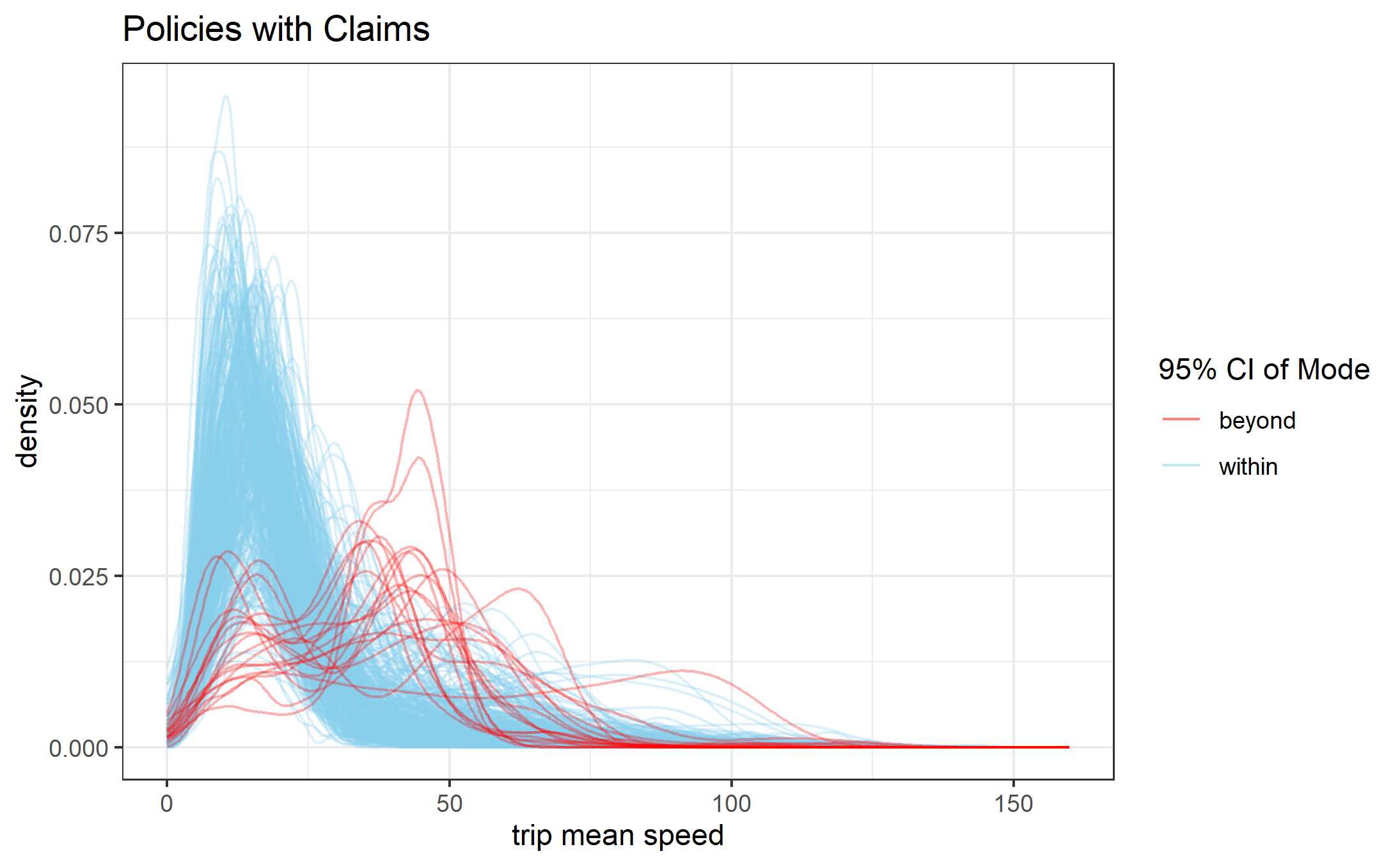
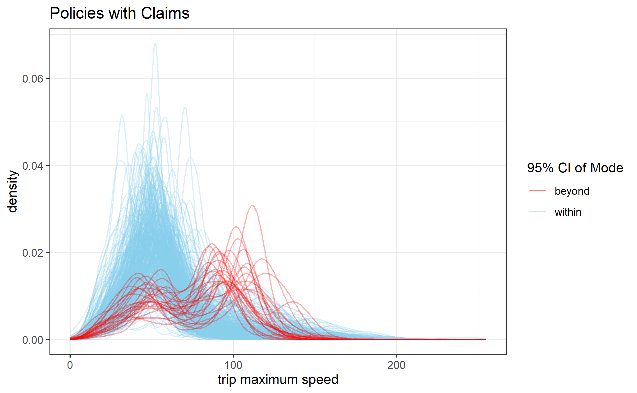
(a)

(b)

Figure 6: Trip-based Maximum Speed for Policies With and Without Claims; Simple Clustering Based on Whether the Mode is Within (Blue) or Beyond (Red) 95% Confidence Interval of the Group.

(a)

(b)

Figure 7: Sample Driving Behaviour (Trip Mean and Maximum Speed) and the Corresponding Speed Transition Matrix.

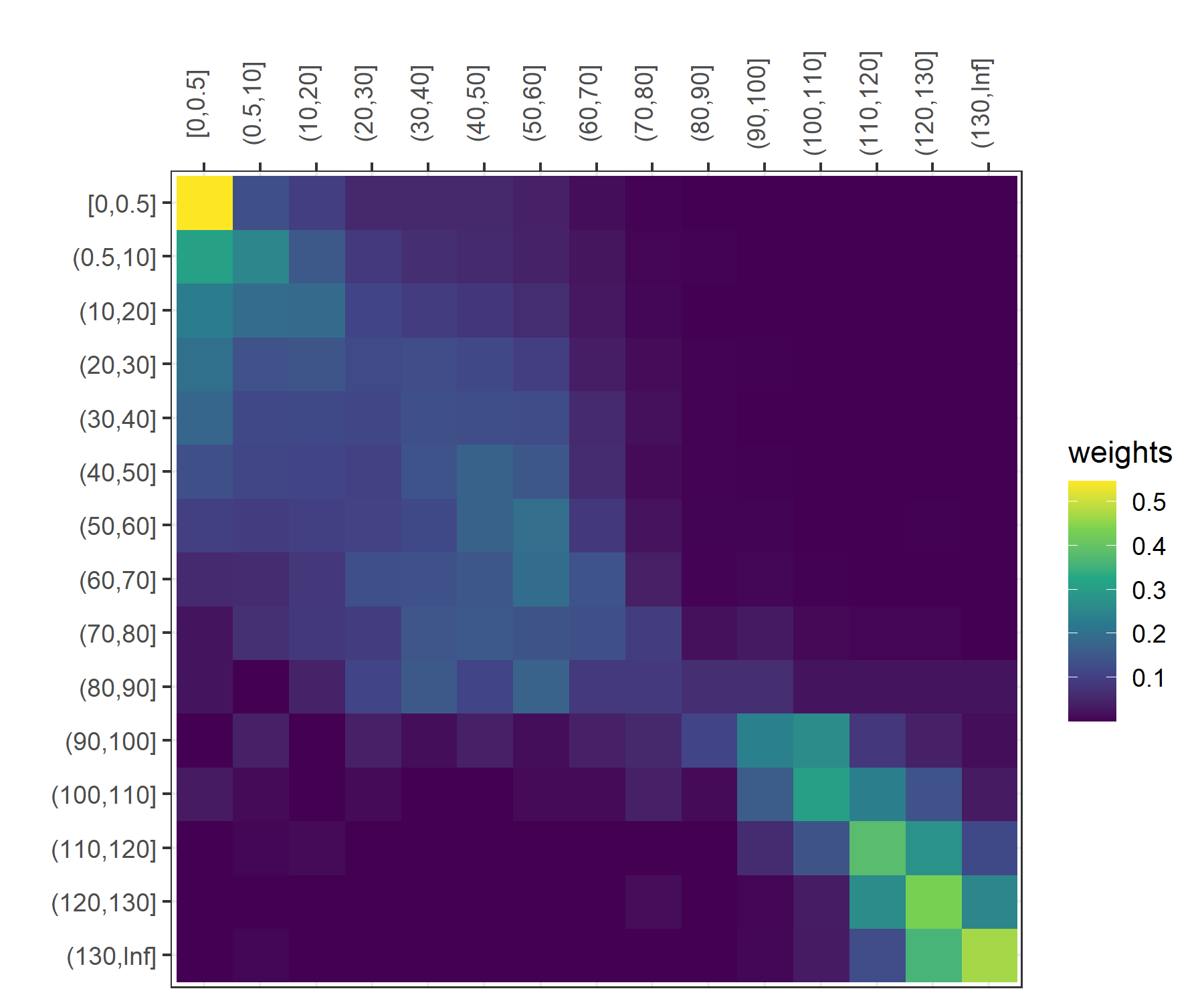
Driver A

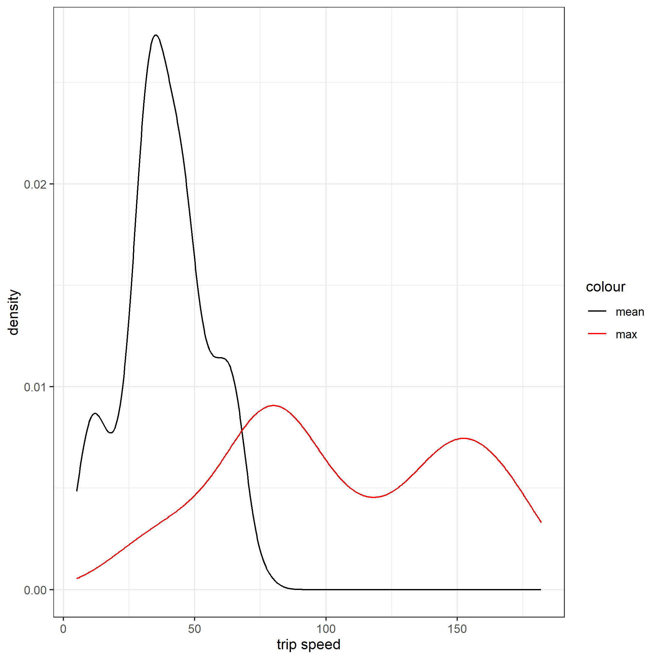
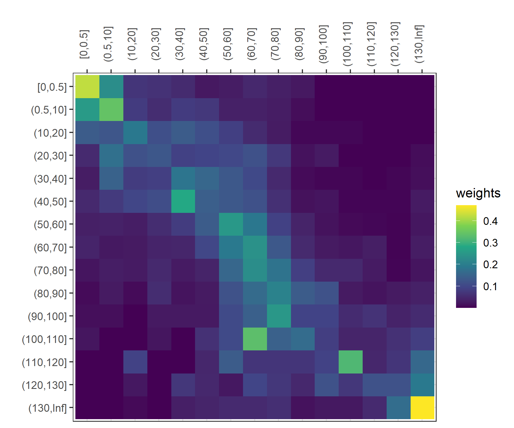
Driver B

Figure 8: Sample Driving Behaviour I - Over Time: Left - Mean Speed, Mid - Maximum Speed, Right - Trip Starting Hour

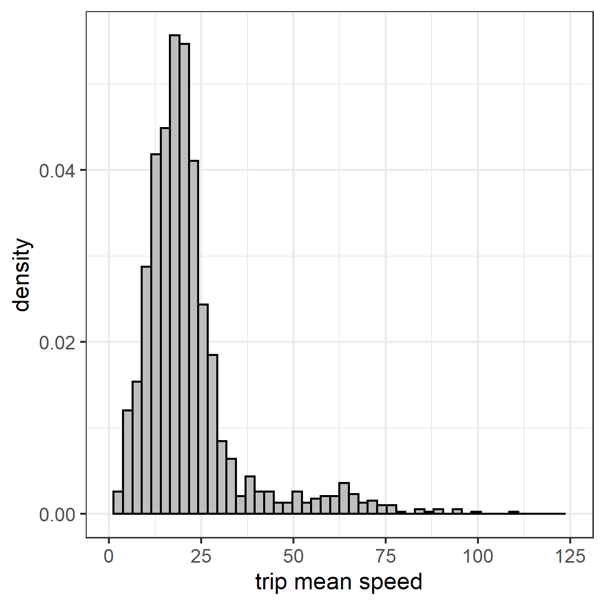
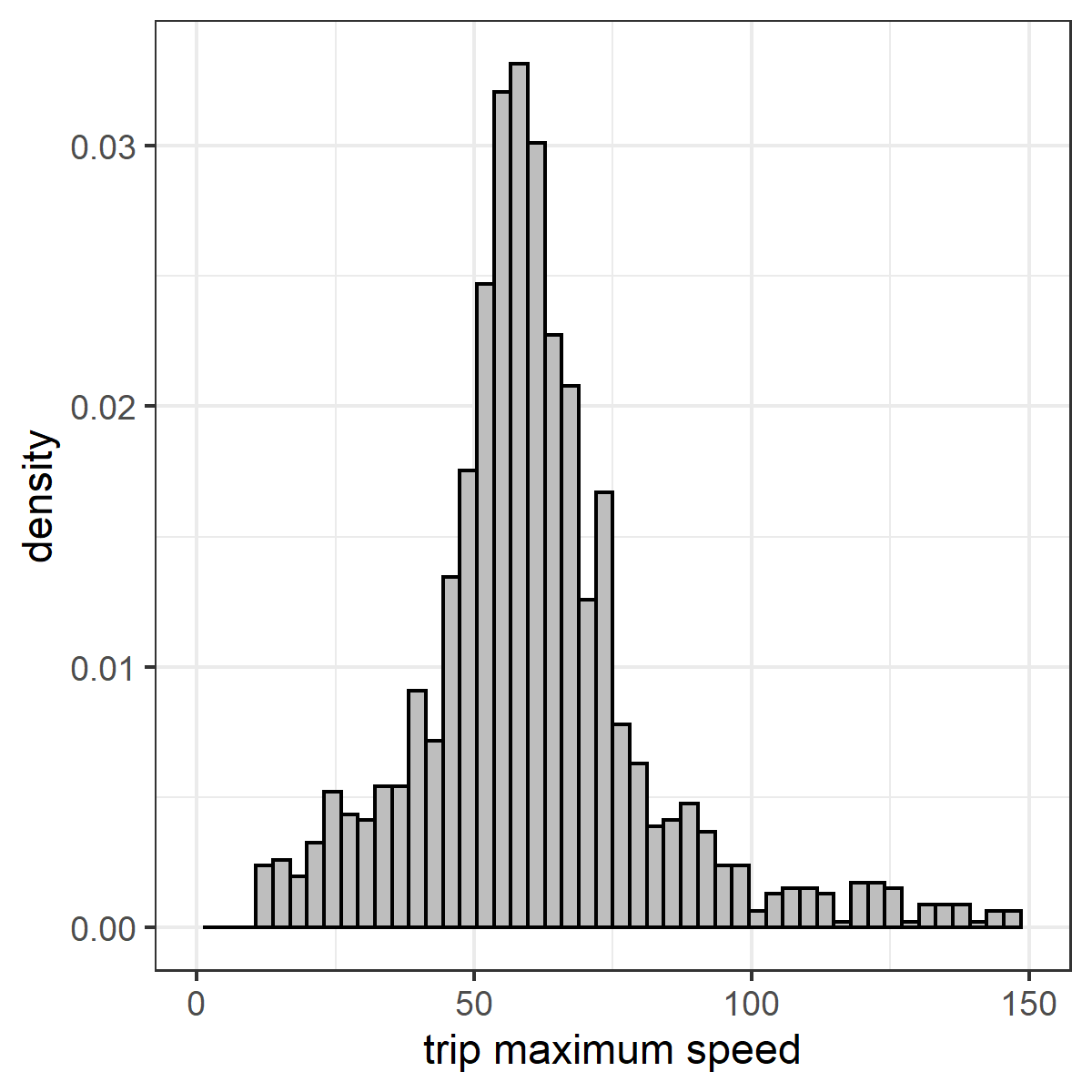
(a) Driver C in 2018 - 0 Claims

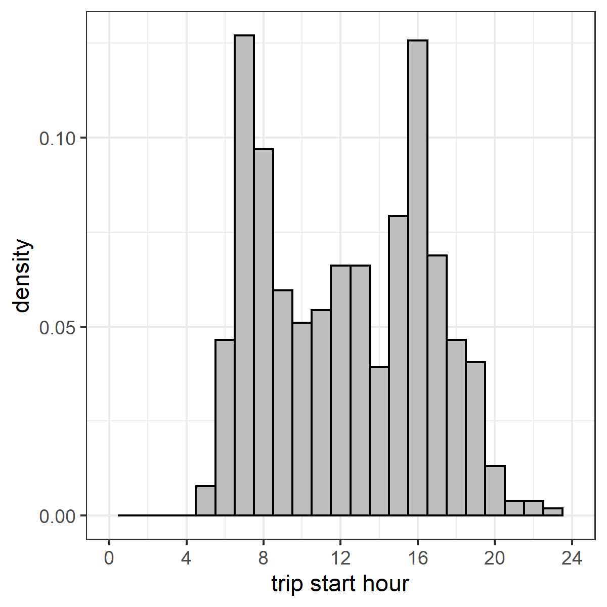
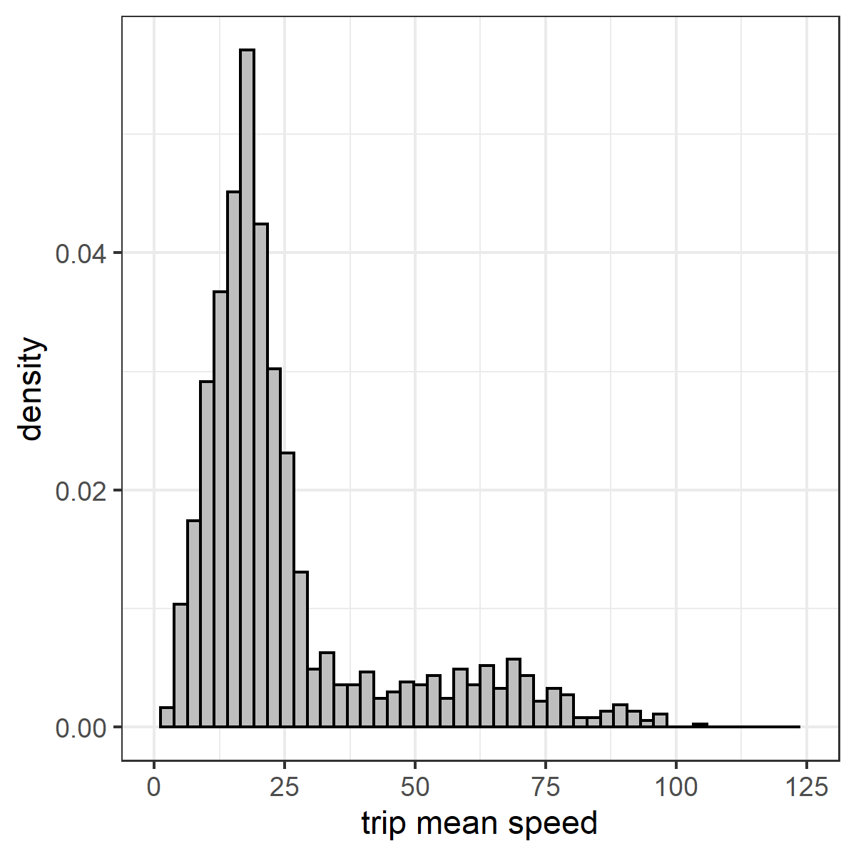
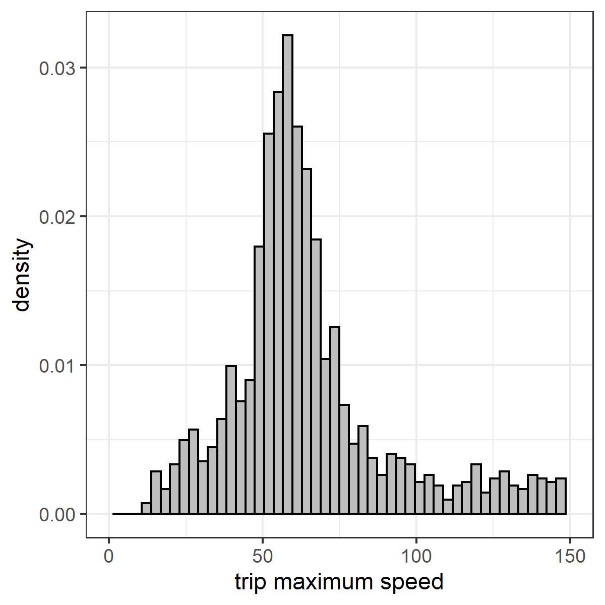
(b) Driver C in 2019 - 2 Claims

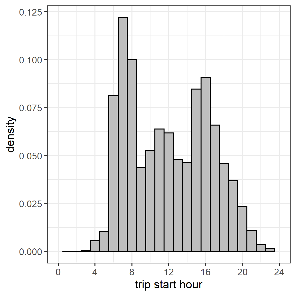
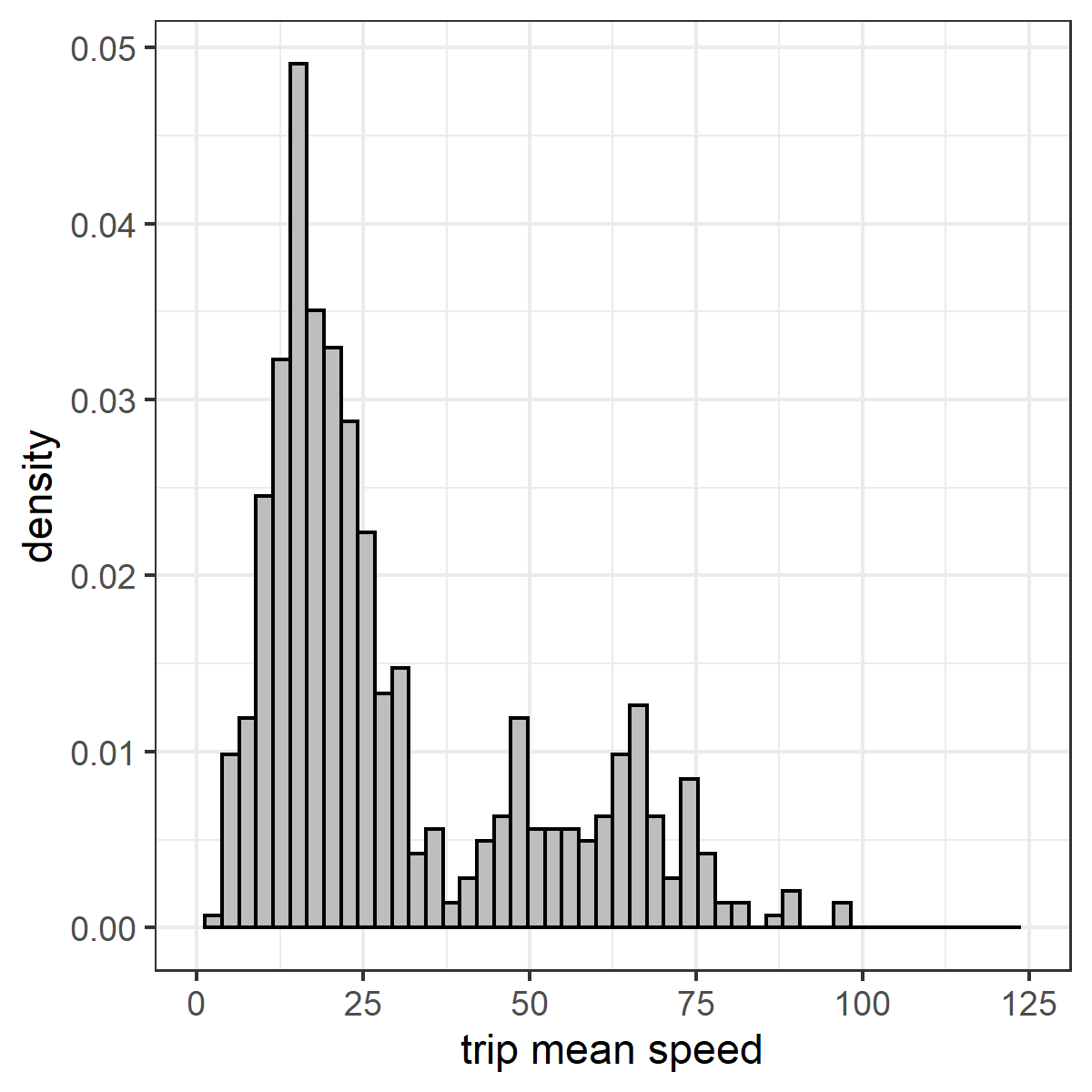
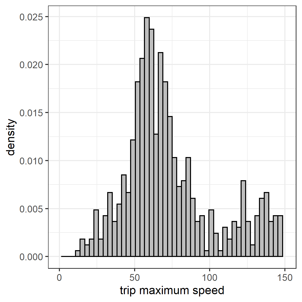
(c) Driver C in 2020 - 0 Claims

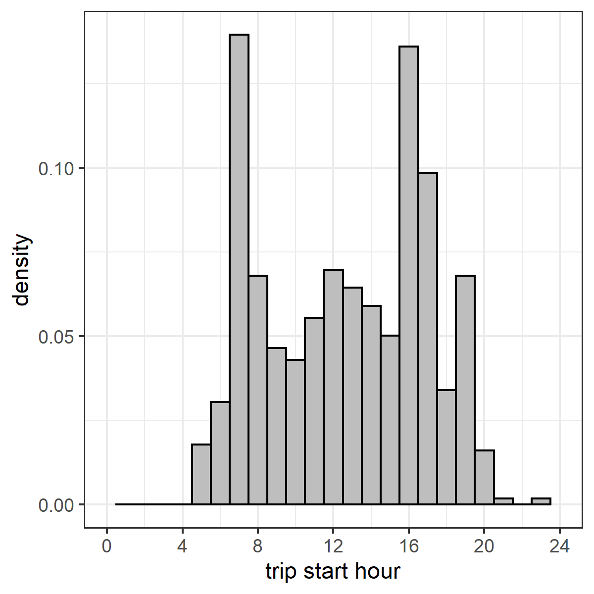
Figure 9: Sample Driving Behaviour II - Over Time: Left - Mean Speed, Mid - Maximum Speed, Right - Trip Starting Hour

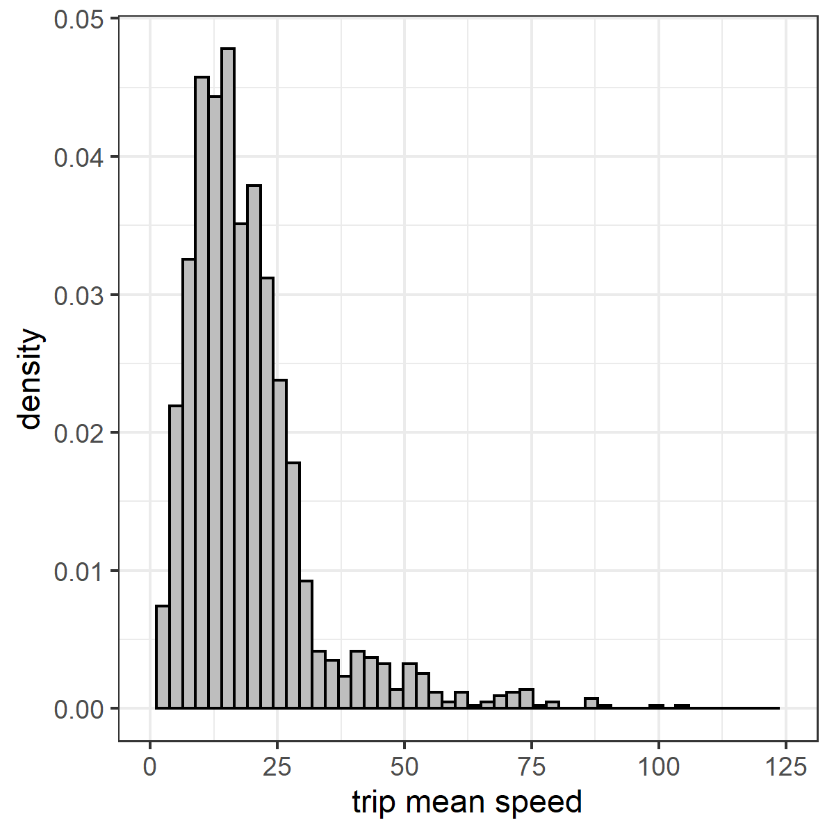
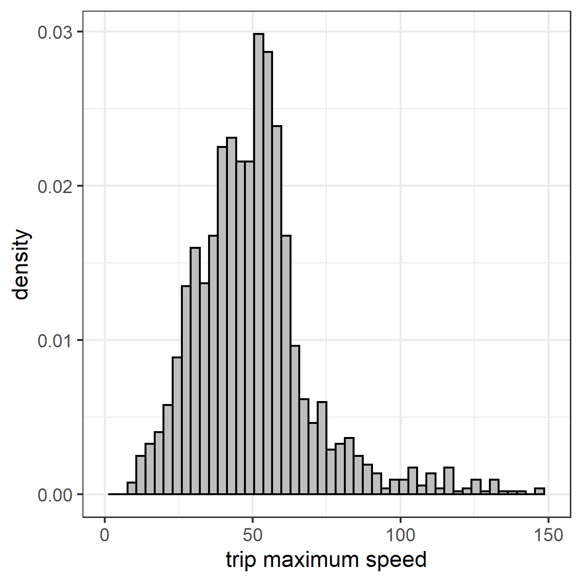
(a) Driver D in 2018 - 0 Claim

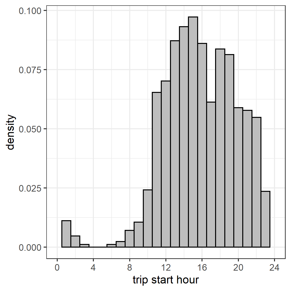
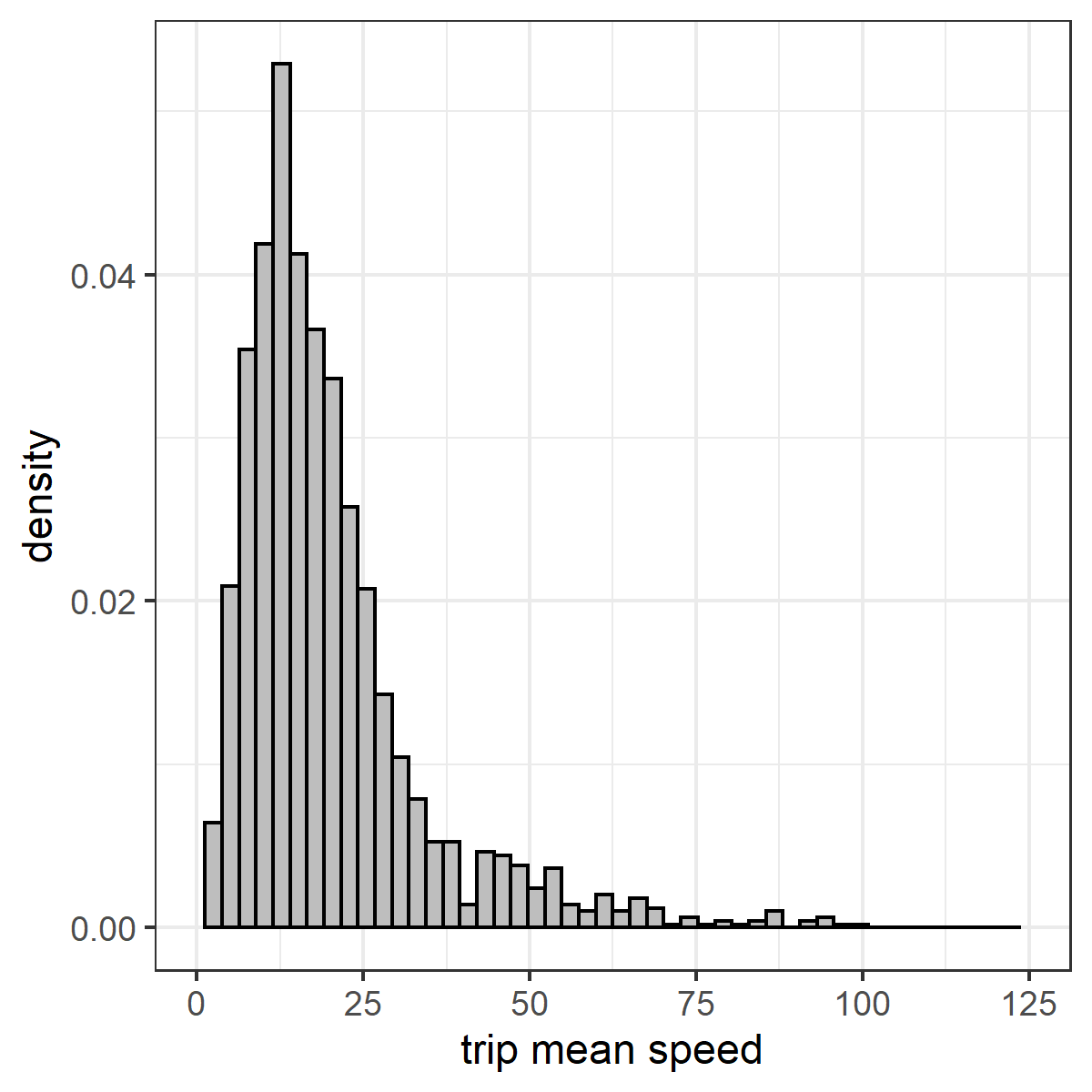
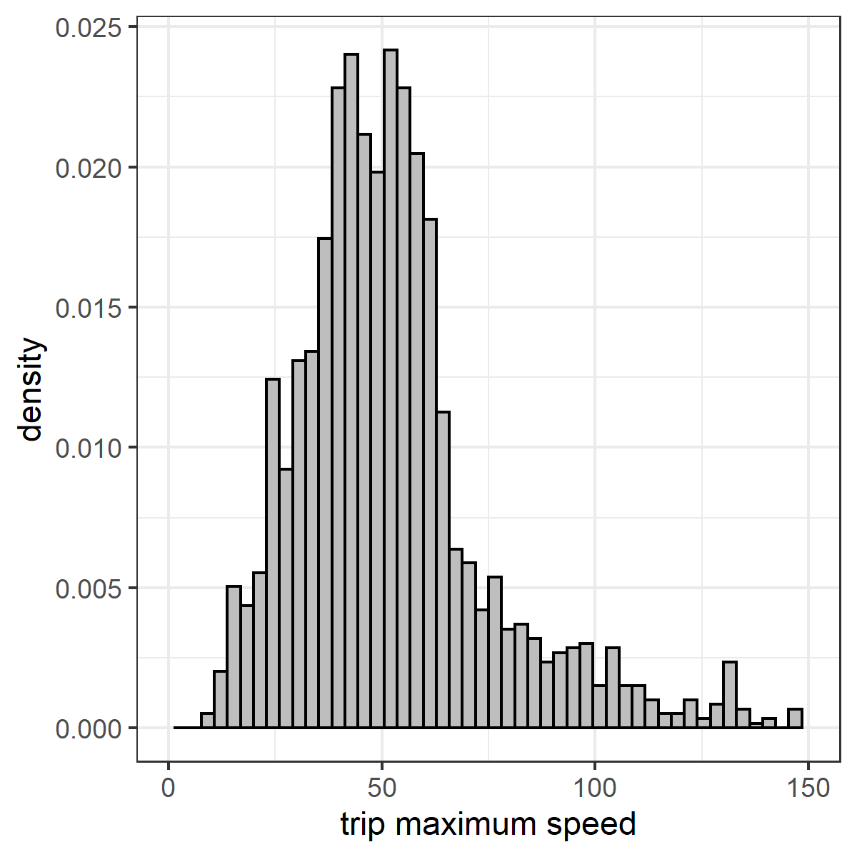
(b) Driver D in 2019 - 0 Claim

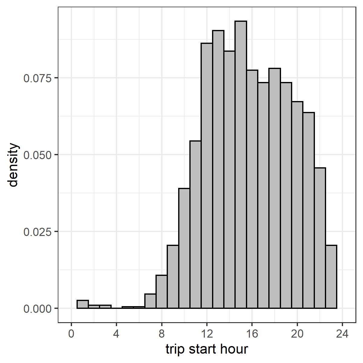
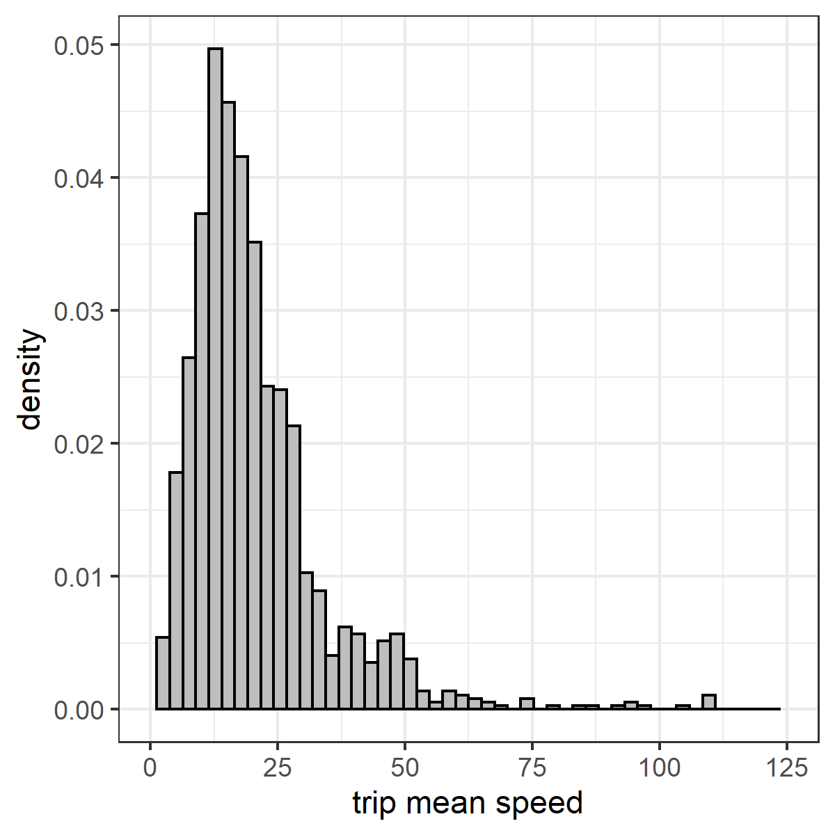
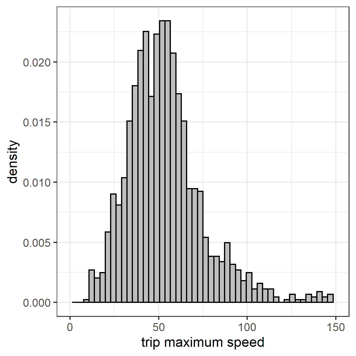
(c) Driver D in 2020 - 0 Claim

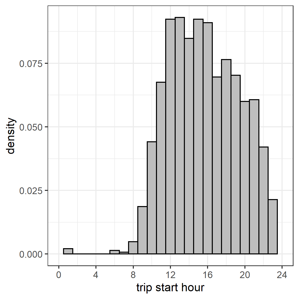
4 Negative Binomial Generalized Linear Models and Drivers’ Learning Effects

This section analyzes the relationship between claim counts (response) and various covariates, both the traditional and the telematics ones. In particular we will consider the Negative Binomial Generalized Linear Model (GLM) and perform feature selection via a 5-fold cross-validation.

4.1 Empirical Evidence of Drivers’ Learning Effects from Telematics Data

Before we model the claim counts, we first study the harsh event arrivals to understand how driving behaviour is changing. Harsh driving events may be considered as ‘near-misses’. A near-miss can be defined as ‘sudden braking and rapid steering operations by the driver without resulting an accident’ (Arai et al., (2001)). Aside from modelling claim probability and claim counts with near-misses, several literatures have also considered the modelling of near-misses, considering them as proxies for the rarely observed claim arrivals (Guillen et al., (2020), Sun et al., (2020), Sun et al., (2021)). A good definition of near-miss events is itself a research topic, and questions include what the detection threshold of harsh events should be and how closely related the near-misses and claims are. In our data, harsh driving events and their detection thresholds are predetermined. Our empirical results show that it takes increasingly longer for a severe harsh event to arrive as total driving time increases, while there is little to no change for other harsh events detected at a lower threshold. This may be how learning effect - the idea that as drivers spend more time on the road, they become more experienced and can react to road conditions better - is reflected in driving behaviour. While we have not found a formal definition of learning effect in the literature, in our analysis, we define it as the decreasing rate of severe harsh event arrivals as cumulative driving time (or distance) increases.

For each policy, we record the rank, type and cumulative driving time of each detected harsh event. We have five types of harsh events: harsh acceleration, harsh braking, left cornering, right cornering and severe harsh events. Recall that the first four types are detected at a lower threshold of 0.5G and the last type is detected at 1.5G. For each type, we perform a linear regression on the log-log scale:

$$\ln(\hat{y}_{ij}) =\hat{\alpha}+\hat{\beta}\ln(t_{ij})$$

$$\hat{y}_{ij} =(t_{ij})^{\hat{\beta}}\times\exp(\hat{\alpha})$$

where for event type $j$, $\hat{y_{ij}}$ is the expected rank of harsh event of policyholder $i$, which is also the expected number of harsh events to date, and $t_{ij}$ is his/her cumulative driving time. While linear regression is not the best model for discrete event numbers, our aim here is merely to fit a trend between harsh event arrivals and cumulative driving time. As the total number of harsh events can only increase with time, the coefficient $\hat{\beta}$ must be positive. In particular, if $\hat{\beta}$ is close to 1, the relationship between harsh event arrivals and total driving time is directly proportional, whilst if $\hat{\beta}$ is significantly less than 1, it takes increasingly longer for an event to arrive as total driving time increases which demonstrates some learning effect.

The fitted coefficients for each type of harsh event is shown in Table 9. As the telematics observation period for each policy varies, the total number of harsh events also varies. To ensure robustness of our analysis, we filter for the event numbers where there are at least five occurrences (e.g. $y_{1000,j}$ is retained if at least five policies have reached 1000 harsh event type $j$). We observe that $\hat{\beta}$ ranges between 0.78 and 1.03 for the first four types of harsh events, while it is significantly smaller for severe events, ranging between 0.26 and 0.49. Moreover, we also investigate if there is a difference in the behaviour of drivers with and without claims. While the general trends are similar, we observe that the coefficients fitted from policies with claims are all larger than those fitted from policies with no claims.

The results can be interpreted as learning effect. As drivers spend more time on the road, they become more experienced and can react to road conditions better. As a consequence, there are less severe harsh events occurring as cumulative driving time increases. However, no matter how experienced a driver is, not all harsh events can be avoided in reality, and some of them may actually be necessary, such as harsh braking to avoid a collision (Guillen et al., (2021)). Hence, we do not see a change as significant for the harsh events detected at a lower threshold. Moreover, we observe that riskier drivers (who filed at least one claim) demonstrate a smaller learning effect than safer drivers in general. Their more aggressive and unimproved driving behaviour may be one of the many factors that contributes to claim occurrence.

Table 9: Fitted Coefficient $\hat{\beta}$ for Each Type of Harsh Event: a coefficient close to 1 shows little to no learning effect, while a coefficient significantly less than 1 demonstrates existence of learning effect. Rows indicated as $\geq 5$ refer to the event numbers where there are at least five occurrences.

		Acceleration	Deceleration	Left Cornering	Right Cornering	Severe Event
All Policies	all	0.9455	0.9390	1.0272	0.9312	0.4430
	$\geq 5$	0.7920	0.9101	0.8925	0.7789	0.2872
No Claim	all	0.9058	0.9142	0.9056	0.8308	0.4291
	$\geq 5$	0.7340	0.8664	0.8144	0.7576	0.2632
Claimed	all	0.9831	0.9591	1.1361	1.0349	0.4878
	$\geq 5$	0.8449	0.9526	0.9646	0.7976	0.3630

• Under the Wald test, all estimated coefficients are statistically different from 1 with significance level of 0.5%.

4.2 Motivation for Using the Negative Binomial

While various literatures have employed the Poisson regression in modelling claim counts (Boucher et al., (2017), Ayuso et al., (2019), Huang and Meng, (2019), Guillen et al., (2021), Gao et al., 2022b ), we propose to use the Negative Binomial GLM instead. First, the choice of Negative Binomial distribution is motivated by the existence of zero-inflation in the claim data, which will lead to an overdispersion with respect to Poisson distribution. Our claim count has a sample mean of 0.4465 and a sample variance of 0.7909. Clearly the widely used Poisson GLM is not a proper candidate model in this situation. Second, the use of GLM instead of more flexible models such as a Generalized Additive Model (GAM) is to prevent overfitting, especially when the number of observations is limited compared to the number of covariates.

Our first analysis compares the Poisson and the Negative Binomial GLMs, both using a log link function and taking into account only the traditional covariates (with policy_period as the offset and region2 as the location factor covariate). We assess both the goodness-of-fit and predictive power of the two models with a 80-20 train/test split. The train and test sets have close sample means (0.4490 and 0.4364 respectively) to ensure that the latter is representative of the original data, and hence is a set on which out-of-sample testing is valid. In Table 10 we report the in-sample and out-of-sample Root-Mean-Squared-Error (RMSE) and Mean-Absolute-Error (MAE) one usually looks at in out-of-sample testing. While the performances of both models seem close, RMSE and MAE are susceptible to outliers, hence we also reported the Chi-Square Statistics, given by

$$\chi^{2}=\sum_{i=0}^{n}\frac{(O_{i}-E_{i})^{2}}{E_{i}}$$

where for each bin $i$ (i.e., the unique claim numbers $0,1,2,...,n$), $O_{i}$ is the observed value and $E_{i}$ is the expected value from the fitted model. As revealed by the in-sample and out-of-sample Chi-Square Statistics in Tables 11 and 12 respectively, in fact Poisson GLM has a worse fit as it misses both the zero-inflation and the right-tail.

Table 10: Model Performance of Poisson and Negative Binomial GLMs

		Poisson GLM	Negative Binomial GLM
	RMSE	0.8879	0.8939
In-sample	MAE	0.6320	0.6320
	Chi-square	414.2863	3.5415
	RMSE	0.8478	0.8514
Out-of-sample	MAE	0.6180	0.6168
	Chi-square	155.5979	5.1729

Table 11: In-sample Chi-Square Statistic of Poisson and Negative Binomial GLMs

Claim count	Observed	Expected
		Poisson GLM	Negative Binomial GLM
0	844	751.88	842.09
1	201	323.91	207.91
2	72	76.16	70.85
3	34	12.86	26.84
4	7	1.84	10.80
5	5	0.28	4.54
6	4	0.07	3.97
Chi-square statistics		414.2863	3.5415

Table 12: Out-of-sample Chi-Square Statistic of Poisson and Negative Binomial GLMs. The binned Chi-square statistics combines the two bins of claim counts 4 and 6 to reduce fluctuation.

Claim count	Observed	Expected
		Poisson GLM	Negative Binomial GLM
0	209	186.84	209.87
1	52	81.18	51.92
2	22	19.23	17.72
3	3	3.24	6.72
4	4	0.44	2.70
6	1	0.06	2.07
Chi-square statistics		56.2159	4.2768
Chi-square statistics (binned)		82.1170	3.7304

4.3 Traditional and Telematics Covariates

To identify the important claim predictors, we perform a 5-fold cross-validation (CV) for different Negative Binomial GLM candidates, each using a (sub)set of the available covariates. In a $k$-fold cross validation, the dataset is split into $k$ subsets. In each fold, the model is trained on $k-1$ subsets, and the trained model is tested on the remaining subset. The $k$-fold CV then reports the average of the $k$ results.

Our dataset is randomly partitioned into 5 subsets such that their mean claim counts are close (0.4364, 0.4192, 0.4573, 0.4384 and 0.4845 respectively), which again ensures that each subset is representative of the original dataset. As we have restricted to the Negative Binomial distribution, on top of RMSE and MAE, we also report the Negative Binomial deviance, which is

$$D=2\sum_{i=1}^{n}\left\{y_{i}\log\left(\frac{y_{i}}{\mu_{i}}\right)+(1+y_{i})\log\left(\frac{1+\mu_{i}}{1+y_{i}}\right)\right\}$$

where if $y_{i}=0$, the term $y_{i}\log\left(\frac{y_{i}}{\mu_{i}}\right)$ is taken to be zero, with $y_{i}$ and $\mu_{i}$ being the $i$-th observation and its prediction respectively. For each of these metrics, a lower value indicates a better performance.

In Table 13 we begin with glm1 which includes all traditional covariates (with region1) but no exposure. In glm2 and glm2b we compare the performance when the exposure policy_period is included, either as an offset (i.e., regression coefficient being 1) or an ordinary covariate. The inclusion of policy_period is clearly beneficial, but the extra flexibility in using it as a covariate does not bring about an improvement in model fit and prediction; hence our analysis proceeds with policy_period as an offset. In glm3 we replace region1 with region2 which has fewer levels. As expected, the new model generalizes better and has a better out-of-sample performance, and so we proceed with region2.

Table 13: 5-Fold Cross-Validation Performance of Models with Traditional Covariates Only.

	Variables	glm1	glm2	glm2b	glm3
Traditional	region1	X	X	X
	region2				X
	max_weight	X	X	X	X
	car_value	X	X	X	X
	num_seats	X	X	X	X
	renewal	X	X	X	X
	use	X	X	X	X
	vehicle_age	X	X	X	X
	policy_period		offset	X	offset
	IS_dev	0.8522	0.8266	0.8243	0.8274
	OS_dev	0.8817	0.8548	0.8527	0.8498
	RMSE	0.8987	0.8960	0.8982	0.8922
	MAE	0.6439	0.6330	0.6323	0.6321

Table 14: 5-Fold Cross-Validation Performance of Models with Traditional Covariates and Telematics Exposure.

	Variables	t_glm1	t_glm1b	t_glm1c	t_glm2	t_glm2b	t_glm2c
Traditional	region1
	region2	X	X	X	X	X	X
	max_weight	X	X	X	X	X	X
	car_value	X	X	X	X	X	X
	num_seats	X	X	X	X	X	X
	renewal	X	X	X	X	X	X
	use	X	X	X	X	X	X
	vehicle_age	X	X	X	X	X	X
	policy_period
Telematics	total_distance	offset	X	logged
	total_time				offset	X	logged
	IS_dev	0.8471	0.8383	0.8209	0.8213	0.8252	0.8107
	OS_dev	0.8737	0.8606	0.8460	0.8463	0.8483	0.8353
	RMSE	1.0367	0.9158	0.8997	0.9203	0.8947	0.8891
	MAE	0.6416	0.6399	0.6234	0.6193	0.6281	0.6178

Table 15: 5-Fold Cross-Validation Performance of Models with Both Traditional and Telematics Covariates. tm indicates telematics and speed transition matrix, while tt indicates the former two and driving time.

	Variables	t_glm3	t_glm4	tm_glm1	tm_glm2	tt_glm1	tt_glm2
Traditional	region1
	region2	X		X		X
	max_weight	X		X		X
	car_value	X		X		X
	num_seats	X		X		X
	renewal	X		X		X
	use	X		X		X
	vehicle_age	X		X		X
	policy_period
Telematics	prop_roadtype	X	X	X	X	X	X
	avg_speed	X	X	X	X	X	X
	max_speed	X	X	X	X	X	X
	pc1			X	X	X	X
	pc2			X	X	X	X
	prop_time					X	X
	num_acc	X	X	X	X	X	X
	num_brake	X	X	X	X	X	X
	num_left	X	X	X	X	X	X
	num_right	X	X	X	X	X	X
	num_severe	X	X	X	X	X	X
	total_distance
	total_time	logged	logged	logged	logged	logged	logged
	IS_dev	0.7949	0.8099	0.7885	0.8011	0.7817	0.7941
	OS_dev	0.8359	0.8297	0.8322	0.8242	0.8346	0.8269
	RMSE	0.8956	0.9024	0.8882	0.8875	0.8858	0.8825
	MAE	0.6162	0.6200	0.6111	0.6137	0.6070	0.6100

We then begin to include telematics covariates. In Table 14 we replace policy_period with either total_distance travelled (t_glm1, t_glm1b and t_glm1c) or total_time driven (t_glm2, t_glm2b and t_glm2c) as the exposure. In each case, exposure is included either as an offset or an ordinary covariate (with or without taking logarithm). Several observations can be made: first, logged expected claim counts seems to have a linear relationship with the logged exposure rather than with the original feature, since the models with the original performed worse; second, both total driving time and distance are better exposure features compared to policy period as they provide a better picture on the extent of vehicle usage. As the models using total time perform better than those using total distance, our analysis proceeds with logged total_time as a covariate; more discussion on this decision (as opposed to including it as an offset) and result is given in Section 4.5.

In Table 15, t_glm3 includes both traditional and telematics covariates (except transition matrix and proportions of driving in different timeslots), whilst t_glm4 includes only telematics covariates. tm_glm1 and tm_glm2 build on t_glm3 and t_glm4 respectively, and include the first two PCs of the speed transition matrix pc1 and pc2. tt_glm1 and tt_glm2 further include the proportions of driving in different timeslots prop_time. While the inclusion of telematics covariates has improved model performance, it is yet unclear what the best model is due to the excessive number of covariates. Hence we proceed to perform feature selection.

One of the most commonly used variable selection method for GLMs is the stepwise algorithm. However, since we evaluate each model via a 5-fold cross-validation, how a stepwise selection should be performed is not immediately obvious. We employ a majority voting scheme: first, stepwise both-side (forward and backward) selection based on Akaike Information Criteria (AIC) is performed on the training set in each fold, and the selected features are recorded; then, the total number of times a feature has been selected (ranging from 0 - not chosen at all, to 5 - chosen in every fold) is summarized, and the features which have been selected more than three times are included in the final model. This can eliminate covariates that are important to only a small portion of the data and reduce overfitting. Based on the finalized subset of covariates, RMSE, MAE and Negative Binomial deviance are calculated on the testing set in each fold. Note that this finalized subset is not necessarily the same subset selected on each fold, e.g. if covariate A is selected four times in total, then there is at least one fold B where its training set does not select this covariate, yet its testing set will be evaluated with this covariate. This should provide a fairer assessment of model performance.

We perform the majority voting procedure on various sets of covariates and the voting results are shown in Table 16. We state explicitly the zero votes to identify the covariates included for stepwise selection. The set of selected features may differ depending on what covariates are included as they compete to explain the most variability in the response. The important traditional covariates are vehicle usage, maximum weight and (monetary) value of the vehicle, whilst to our surprise, vehicle age is relatively unimportant. Maximum speed and number of harsh braking are the more important telematics covariates. However, in the presence of speed transition matrices and driving in different timeslots, which have become the most important telematics covariates, the importance of maximum speed drops slightly, while average speed is eliminated from the selection. A potential explanation is that not only information about average and maximum speed have been captured by the matrix, the matrix is able to provide even more information on the driving speed. It is noteworthy that in tt_glm1ss, number of harsh braking falls just below three votes (the majority criteria) while number of severe events receives one vote. Due to the dependence between the different timeslots and harsh event rates, the former may have captured the predictive power of the harsh events. Although the first PC, by definition, explains the most variability in the transition matrix, it is the second PC that provides the most predictive power for the response. Driving in different roadtypes and numbers of other harsh events are deemed unimportant in all models.

We observe that best out-of-sample deviance is attained by tm_glm1s which includes PCs, while best out-of-sample RMSE and MAE are attained by tt_glm1s which includes both PCs and the driving timeslots. By comparing glm3s to t_glm4s, tm_glm2s and tt_glm2s, we observe that the models with only telematics covariates can already outperform the models with only traditional covariates, but the best performance is attained by a combination of both after all. This verifies the benefits of adding telematics data to claim prediction, but the value of traditional covariates, such as the characteristics of the vehicle, still cannot be ignored, especially due to the limitation of our data.

Table 16: 5-Fold Cross-Validation Performance of Models Resulted from Majority Votes. Covariates with a number are included for stepwise selection, whilst covariates with three votes and more are included in the final model. policy_period is included as an offset in the first model, and logged total_time is chosen in all the other models.

	Variables	glm3s	t_glm3s	t_glm4s	tm_glm1s	tm_glm2s	tt_glm1s	tt_glm2s
Traditional	region1
	region2	0	0		0		0
	max_weight	4	5		4		5
	car_value	5	5		4		4
	num_seats	2	0		0		0
	renewal	2	0		0		0
	use	1	5		3		4
	vehicle_age	0	0		0		0
	policy_period	offset
Telematics	prop_roadtype		1	1	0	0	0	0
	avg_speed		2	4	0	0	0	0
	max_speed		5	5	4	5	3	4
	pc1				0	1	0	0
	pc2				5	5	5	5
	prop_time						5	5
	num_acc		0	0	0	0	0	0
	num_brake		4	4	3	4	2	3
	num_left		0	0	0	0	0	0
	num_right		0	0	0	0	0	0
	num_severe		0	0	0	0	1	0
	total_distance
	total_time		logged	logged	logged	logged	logged	logged
	IS_dev	0.8354	0.8056	0.8137	0.7982	0.8059	0.7924	0.7983
	OS_dev	0.8403	0.8174	0.8241	0.8116	0.8138	0.8121	0.8160
	RMSE	0.8914	0.8797	0.8892	0.8725	0.8776	0.8690	0.8740
	MAE	0.6325	0.6102	0.6152	0.6068	0.6105	0.6017	0.6067

In Table 17 we report the estimated regression coefficients of the final model tt_glm1s fitted to the entire dataset. car_value is in dollars of domestic currency, every 10,000 dollars increase in price leads to $\exp(0.01077)-1=1.08\%$ increase in expected claim count. max_weight is in kilograms, and every 10 kilograms increase leads to a small, 0.28% decrease of expected claim count. The reference class of vehicle usage use is ‘others’, hence personal use demonstrates a higher risk. The coefficient estimate of (logged) total_time is 0.62 instead of 1, where the latter will correspond to an offset. Both max_speed and pc2 have a positive effect on expected claim counts. As explained in Section 3.3, pc2 has small, negative values along the diagonal of the matrix, which are the moderate speed bins and closer transitions, hence an increase in pc2 actually represents reduced stability in speed transitions. Finally, as we have excluded prop_20_24, it acts as the reference group and all other proportions should be interpreted with respect to it. As all the other coefficients are negative, driving in all other timeslots is expected to be less risky than driving between 8 p.m. to midnight.

Table 17: Estimated Regression Coefficients of Selected Model

	Variables	Estimate	Std. Error	z-value	p-value
Traditional	intercept	-4.0120	1.4940	-2.686	0.0072	**
	car_value	0.000*	0.0000	1.927	0.0540	.
	max_weight	-0.0003	0.0002	-2.192	0.0284	*
	use_personal	0.2127	0.1198	1.775	0.0759	.
Telematics	log(total_time)	0.6155	0.0936	6.575	0.0000	***
	max_speed	0.0038	0.0021	1.835	0.0665	.
	pc2	0.0391	0.0126	3.100	0.0019	**
	prop_0_4	-0.0933	0.0352	-2.650	0.0081	**
	prop_4_8	-0.0325	0.0116	-2.812	0.0049	**
	prop_8_12	-0.0304	0.0118	-2.563	0.0104	*
	prop_12_4	-0.0321	0.0130	-2.474	0.0134	*
	prop_4_8	-0.0387	0.0151	-2.570	0.0102	*

• * Coefficient for car_value is 1.077$\times$ 10^-6

• Significance codes: 0 ‘***’, 0.001 ‘**’, 0.01 ‘*’, 0.05 ‘.’, 0.1 ‘ ’, 1

4.4 Robustness of Speed Transition Matrix to Different Bin Widths

We have used a speed transition matrix with a constant bin width of 10 km/h throughout our analysis. In this section we study the change in the PC’s predictive power (hence model performance) with respect to a change in the bin width, provide suggestions on choosing a good bin width, and illustrate that the predictive power is fairly robust to different widths. While one can definitely choose a different bin width for each of the speed bins, we only study constant bin widths for convenience.

For a bin width of (positive integer) $h$ km/h, we create a $m$-by-$m$ speed transition matrix as: [0, 0.5), [0.5, $h$), [$h$, $2h$), …, [$(m-1)h$, Inf), where $(m-1)h$ is the largest integer less than or equal to 130. While the first bin again captures the stationary state, the last bin may not align with the speed limit. Without loss of generality, we consider the same feature sets in Table 16. For all integer $h$ between 2 to 30, the best out-of-sample deviance is attained by tm_glm1s, and the best out-of-sample RMSE and MAE are attained by tt_glm1s. In Figure 10 we compare the model performances against those of the benchmark model t_glm3s as indicated by the red line, which is the model with only traditional covariates. On the one hand, we observe that the values are all close and well below the benchmark, indicating that the model performance (or predictive power) is fairly robust to different bin widths. On the other hand, the values provide suggestions on choosing a good bin width. First, there should be a balance between information granularity and dimensionality: as we include only the first two PC’s and only the second one has strong predictive power, pc2 cannot capture sufficient variance of the matrix if its size is too large (i.e., $h$ being too small); whilst the matrix cannot capture the transition patterns and becomes uninformative if the bin widths $h$ is too large (e.g., in the extreme case, only [0, 0.5) and [0.5, Inf)). Second, the bin widths also determine how closely we can align with the speed limit 130 km/h, and the model performances are better when $h$ is a factor of 130. For example, while the patterns captured by the PC’s of transition matrices of $h$ being 26 km/h and 27 km/h are consistent, the former produces a better model performance as its last bin aligns with the speed limit. An alignment with the speed limit is preferred as it generally captures speeding events; moreover, as the bin is larger (i.e. when lower bound is much less than 130), the transitions within high speeds are neglected.

Figure 10: Out-of-sample Model Performance with Respect to Different Speed Bin Widths. Red line indicates the performance of the traditional covariates only model t_glm3s.

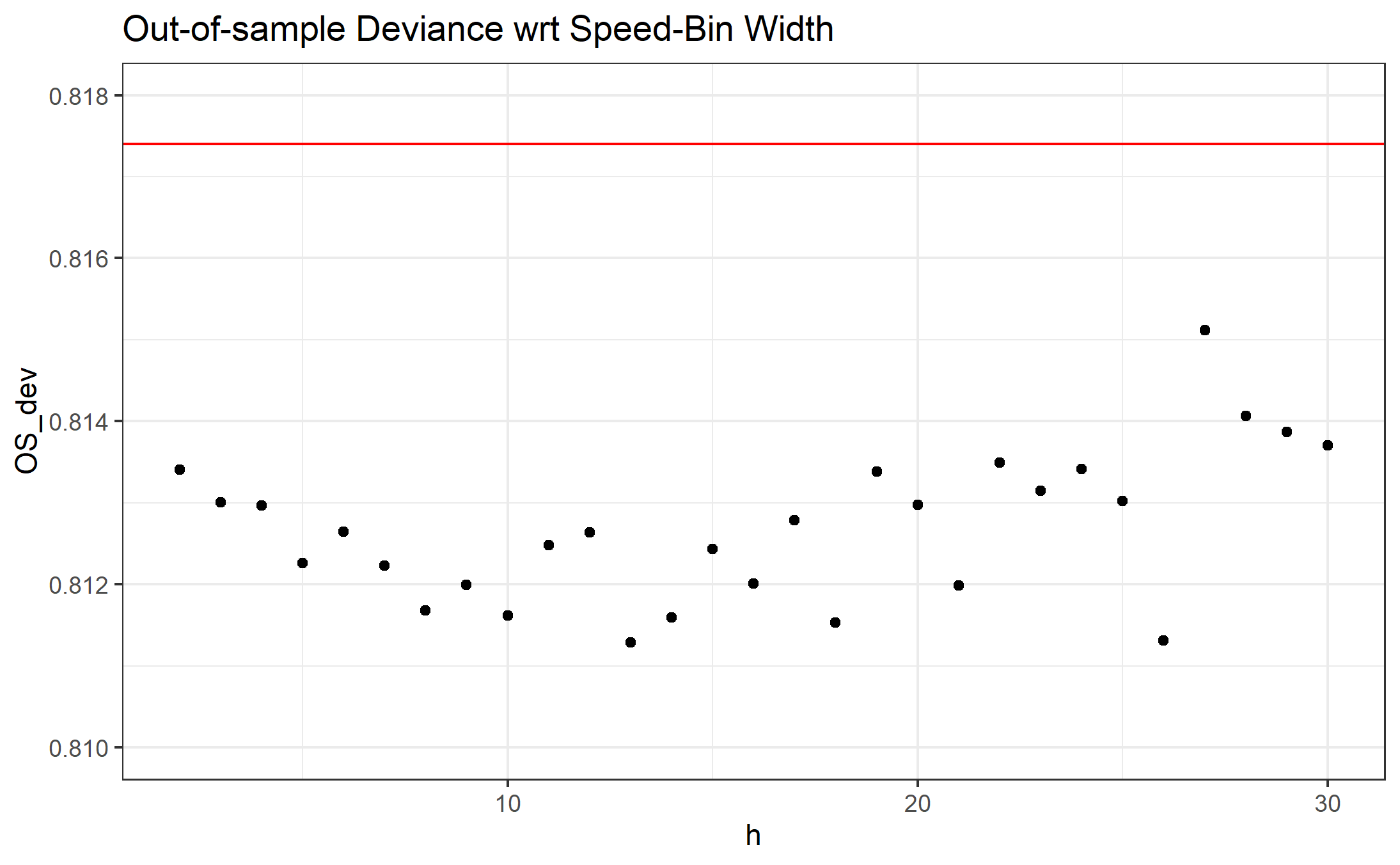
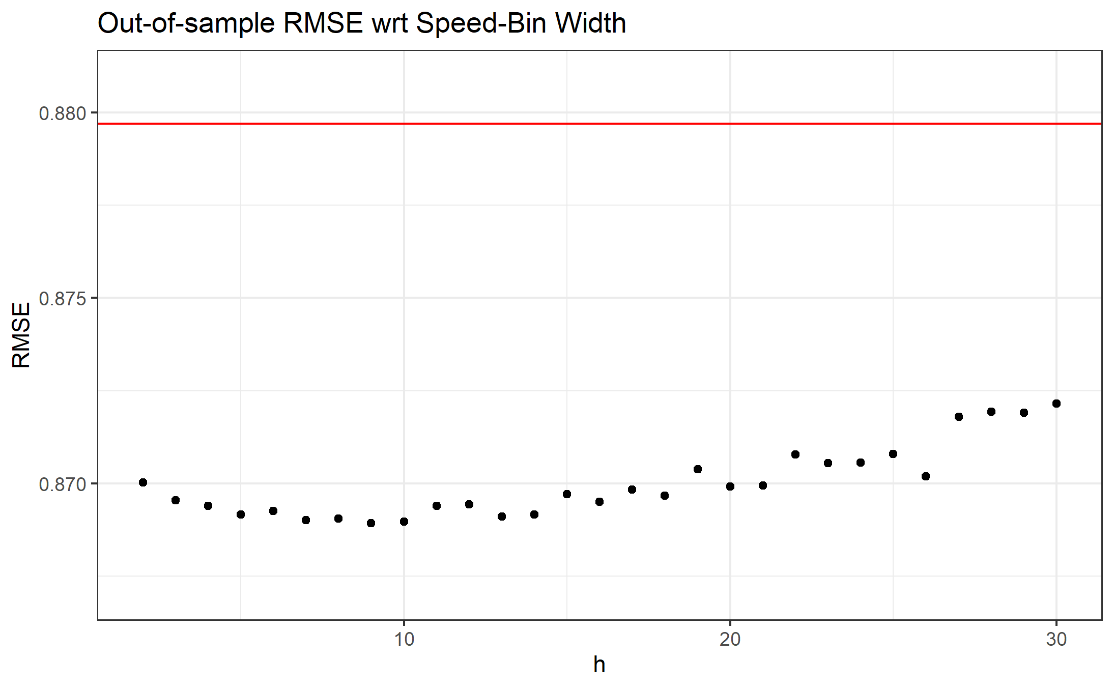
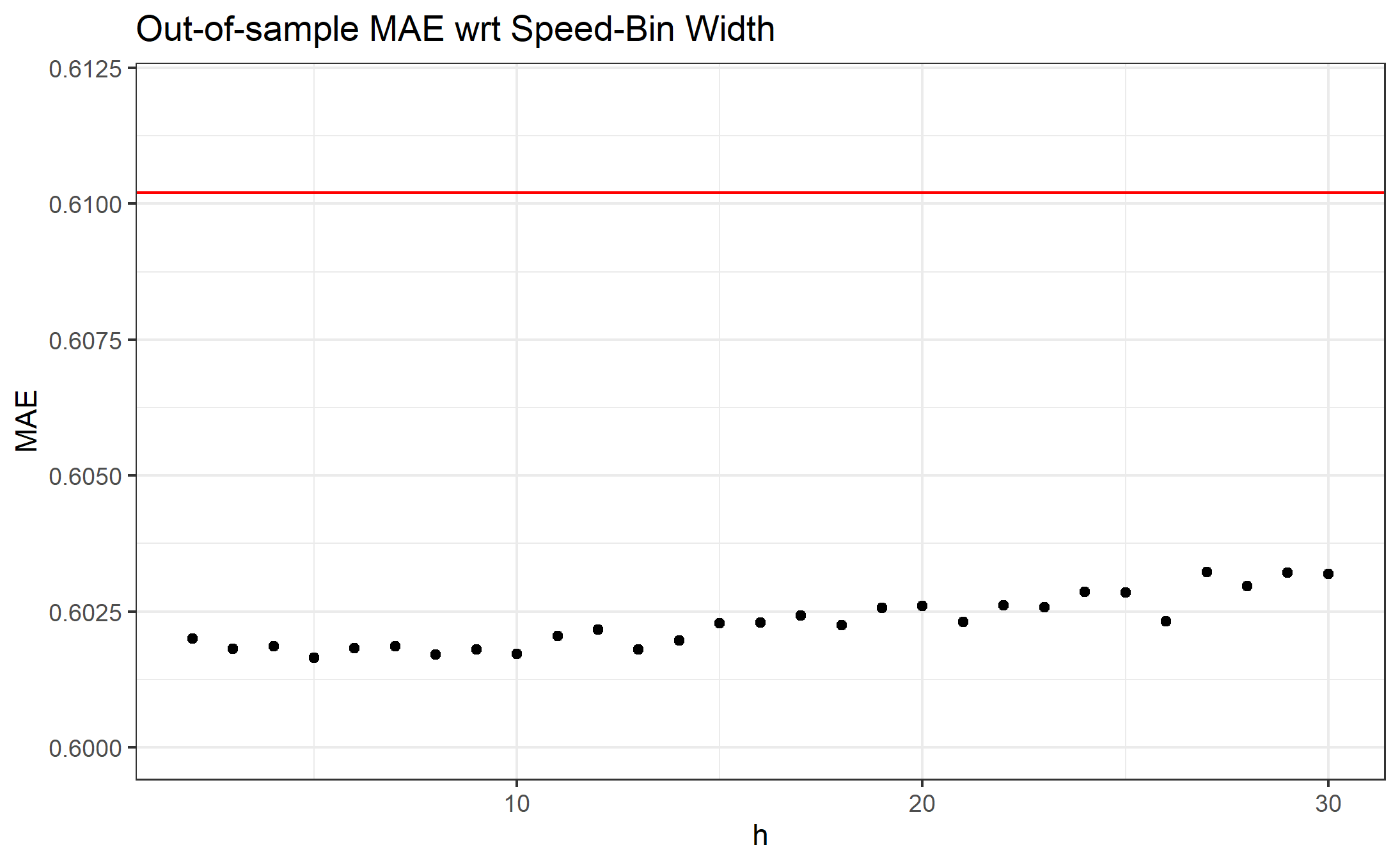
Figure 11: First Principal Component (PC) of Speed Transition Matrices with Different Bin Widths. Patterns are consistent but the (last) bins can be very different.

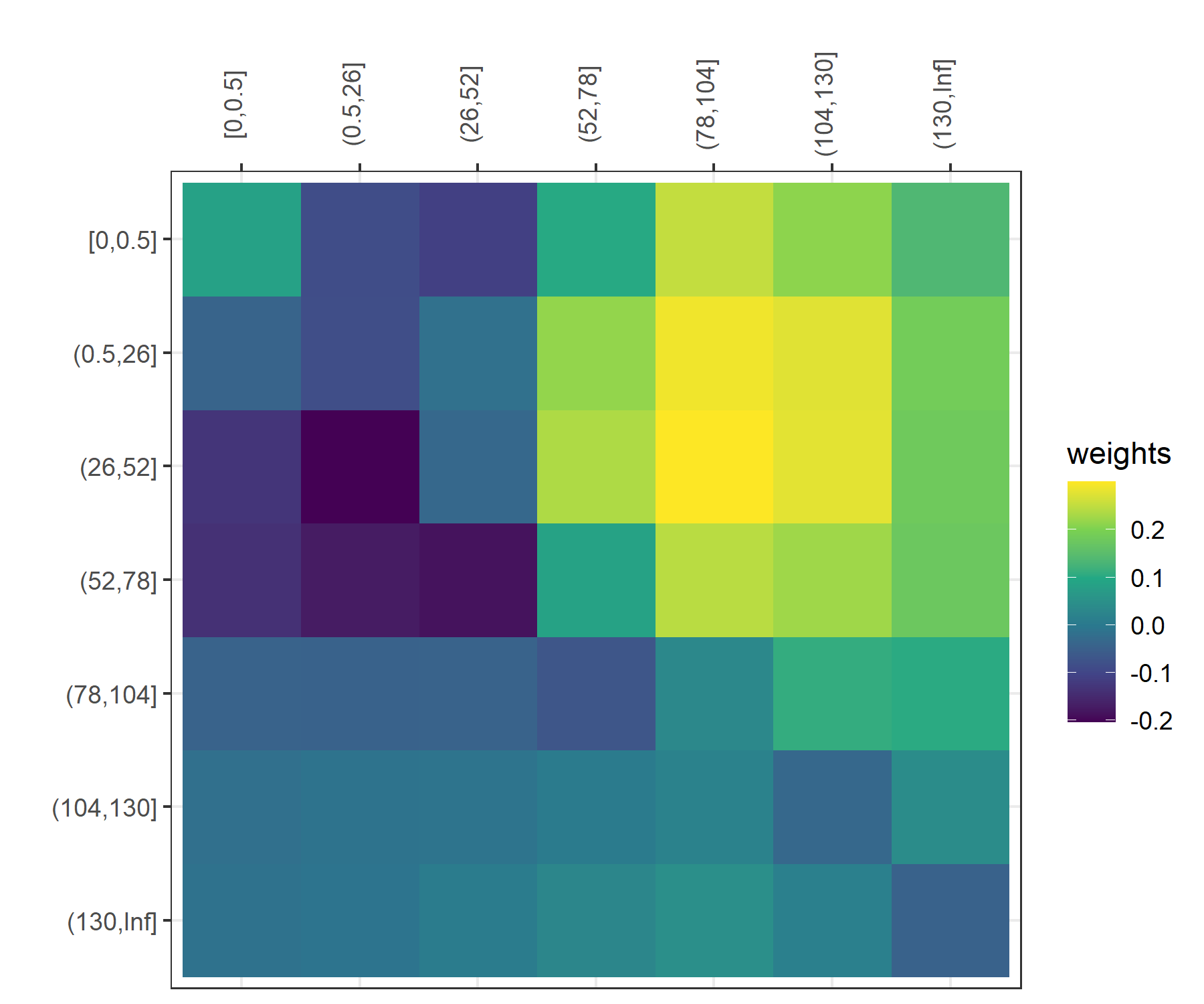
(a) Bin Width of 26 km/h

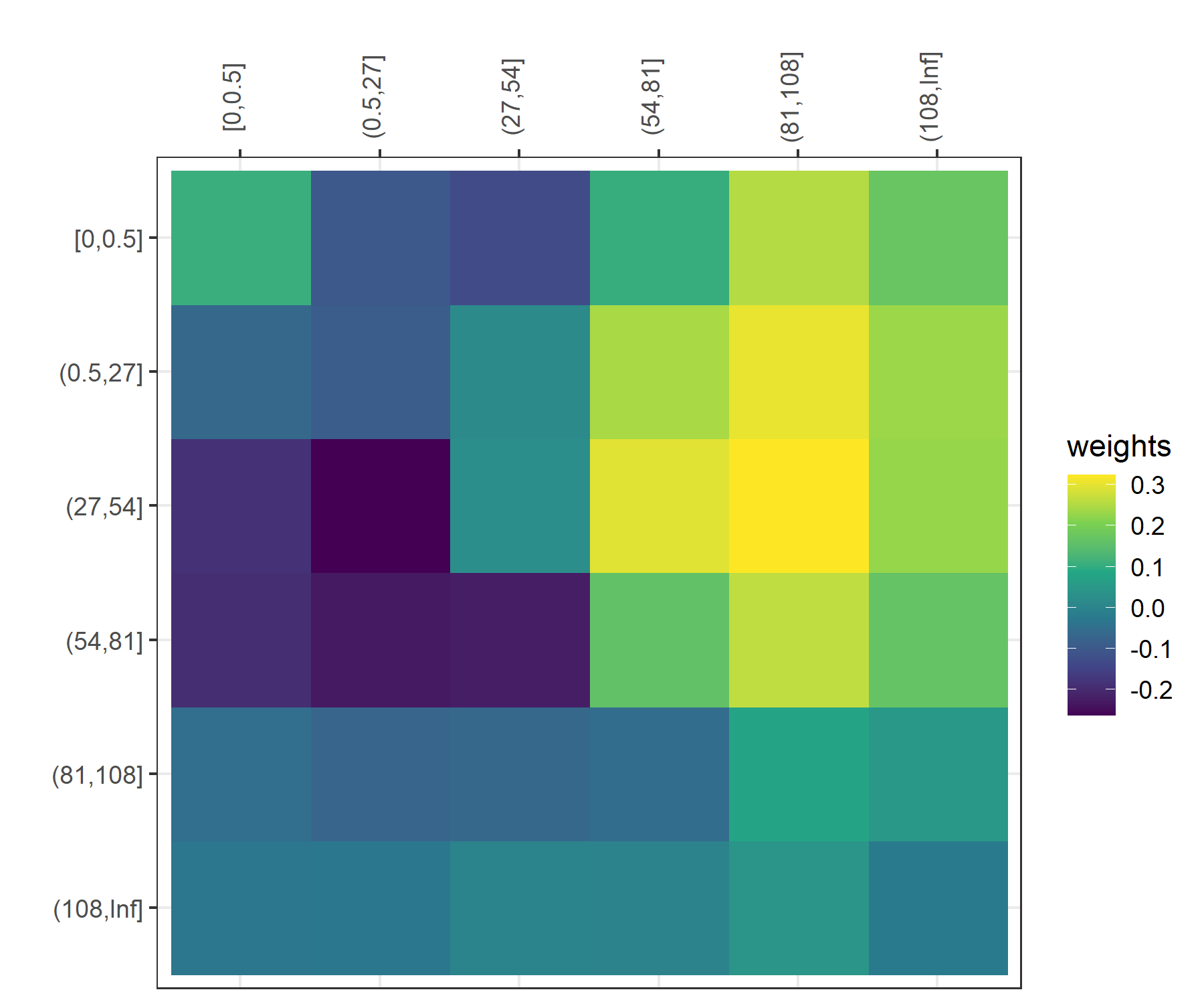
(b) Bin Width of 27 km/h

4.5 Discussions on the Treatment of Total Time or Distance Travelled

In classical ratemaking, policy coverage period is usually treated as an offset in modelling claim frequency, e.g. with coefficient 1 in a GLM. When telematics data becomes available to insurers, this term is usually replaced by total distance travelled. This gives rise to Pay-As-You-Drive (PAYD) Insurance (Boucher et al., (2013) and Paefgen et al., (2014)), in which ratemaking takes into account how much the policyholders drive, in addition to the policyholders’ traditional covariates. While one may continue to use total driving time or distance as an offset (Ayuso et al., (2019), Denuit et al., (2019), Guillen et al., (2021)), some literatures have treated them as a covariate with coefficients estimated from the data (Boucher et al., (2013), Paefgen et al., (2014), Verbelen et al., (2018)). This additional flexibility usually leads to a better model fit. However, discussion on the interpretation behind such model has halted since the rise of Pay-How-You-Drive (PHYD) Insurance - an insurance product which builds on top of PAYD Insurance and considers policyholders’ driving behaviour as well. In this work, we would like to once again raise the attention on the fact that expected claim counts are not directly proportional with total driving time or distance.

In the previous section, we have evaluated models treating total driving time or total distance travelled as an offset, as an ordinary covariate, or as a covariate after taking natural logarithm. Consistent with existing works, model performance is better with the covariate approach. For the best model tt_glm1ss, the coefficients of logged total driving time is 0.6155, regardless of the unit of time. Under the Wald test, this estimated coefficient is statistically different from 1 at significance level of 0.004%. For illustrative purpose, we state the log-link Negative Binomial GLM with coefficient 0.5,

$$\ln(\hat{N}_{i}) =0.5\log(t_{i})+\hat{\beta}_{0}+\hat{\beta}_{1}x_{1i}+\hat{\beta}_{2}x_{2i}+...$$

$$\hat{N}_{i} =\sqrt{t_{i}}\times\exp(\hat{\beta}_{0}+\hat{\beta}_{1}x_{1i}+\hat{\beta}_{2}x_{2i}+...)$$

where $\hat{N_{i}}$ is the expected claim counts for policyholder $i$, $t_{i}$ is his/her total driving time, and $x_{pi}$ are the other covariates of this policyholder. Under this model, claim counts are expected to increase as a function of the square root of total driving time instead of directly proportional. Hence with all other covariates constant, the driver’s riskiness is still increasing with total driving time, but the rate of increase is reducing.

Remark: Since PAYD Insurance is based on mileage instead of driving time, we also report on the relationship between claim counts and mileage for completeness of our analysis. The best model tt_glm1ss is refitted by replacing logged total driving time with logged total distance travelled, and the coefficient is found to be 0.5177. Hence we again conclude that claim counts are expected to increase with mileage, but less than directly proportional.

The same logged covariate structure is employed in Boucher et al., (2013), where the authors consider a Poisson GLM to model claim counts (from different lines of business) but with traditional covariates only. Our results are in line with theirs, where the estimated coefficients of logged total distance travelled are close to 0.5 in all cases. There are two reasons why we do not consider a more flexible function of the covariate, such as the cubic smoothing spline in Boucher et al., (2017). First it does not seem necessary, as shown in Figure 12, where we apply cubic spline on either total time or logged total time alongside the selected covariates from tt_glm1s (in linear form). We observe that cubic spline on total time shows a square-root-like shape, whilst that on logged total time is linear. Hence, a linear relationship between claim counts and logged total time should be sufficient. The second reason is to ensure a monotonically increasing relationship between (expected) claim counts and the total driving time or distance with minimal effort. This is an important condition as the expected claim counts should never decrease with increasing driving. The risk resulted from an earlier part of the trip, say the first 100 km or the first hour driven, should not be affected by the later part of the trip. As a consequence and also given the fact that risk cannot be negative, the overall risk should be at least as big as that resulted from any interval of a trip. Moreover, this condition is relevant from a ratemaking perspective, otherwise policyholders can simply drive infinitely long to minimize their premium.

Figure 12: Best Model tt_glm1s with Cubic Splines on Total Driving Time, Without (Left) and With Logarithm (Right) Applied.

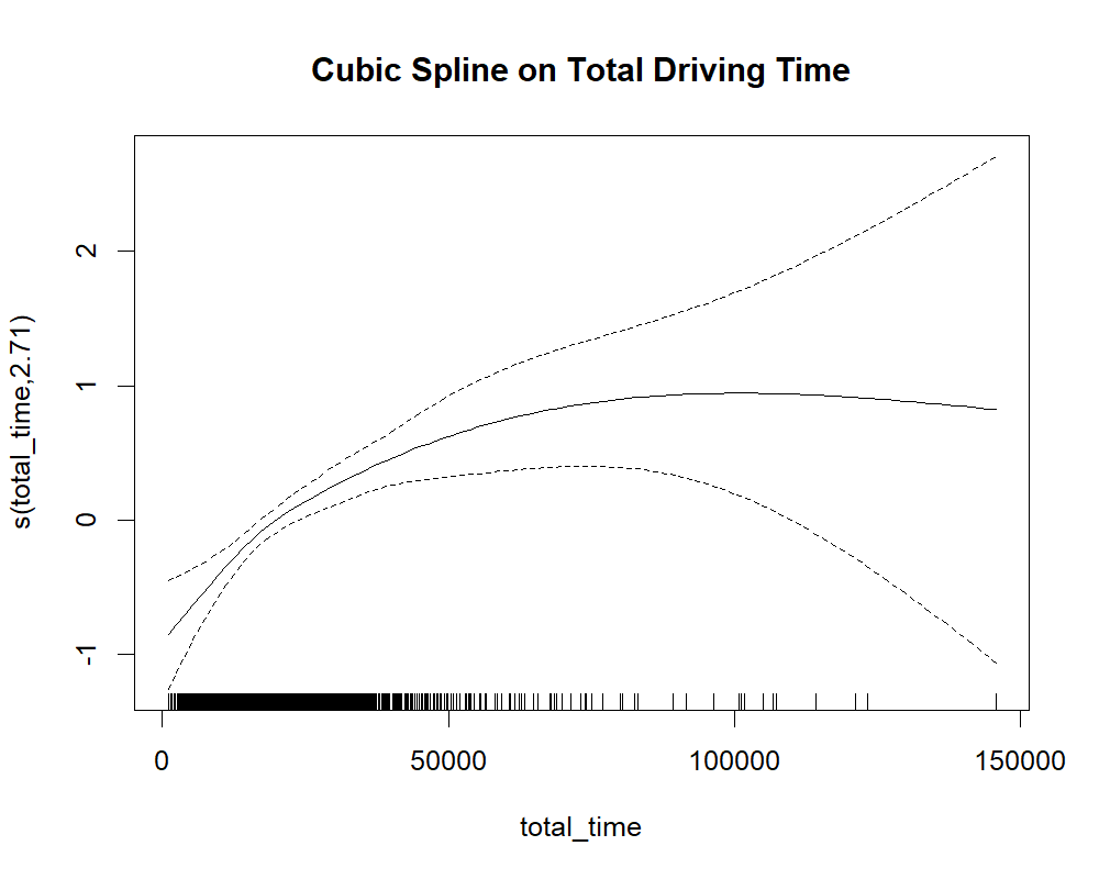
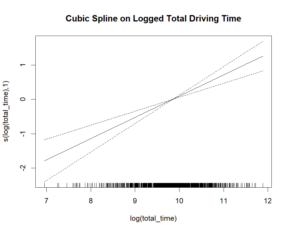
Using a log-link in GLM with a logged covariate is equivalent to fitting a power function of the covariate, hence the relationship is monotonically increasing as long as the fitted coefficient is positive. This observation of average claim counts increasing less than directly proportional to total driving time or total distance travelled is first made in Lemaire, (1985), Litman, (2011) and Joseph Ferreira and Minikel, (2012), where they conclude that a doubling, or even tripling of mileage increases average claim counts by less than a double. One explanation is that the areas travelled can have different riskiness, e.g. familiar neighbourhood versus new destinations. Another explanation is the drivers’ learning effect introduced in Section 4.1. In that section, we have demonstrated a similar, (approximately) square-root trend in severe harsh event arrivals: it also takes increasingly longer for a severe harsh event (detected at 1.5G) to occur as total driving time increases. The gain of experience and improvement in driving behaviour are reflected first in severe harsh event arrivals, and ultimately in claim arrivals.

From a practical perspective, the use of total time or distance travelled as an offset leads to poorer claims modelling and eventually poorer ratemaking. In particular, the use of total driving time as an offset leads to a miss in both tails of the claims distribution when compared to the use of logged covariate. We compare the goodness-of-fit and predictive power of the two models with the same 80-20 train/test split in Section 4.2. By comparing a linear function to a power function with power between 0 and 1, it is clear that the linear function (which is the offset model) underestimates the risk from short-term driving while overestimates the risk from long-term driving. As a consequence, its prediction distribution overestimates both claim 0 and 4+, as shown in Tables 18 and 19, whilst the covariate model gives closer fit and prediction both in- and out-of-sample.

Table 18: In-sample Prediction Distributions of tt_glm1s with Total Driving Time as Offset or (Logged) Covariate.

Claim count	Observed	Expected
		Offset	Covariate
0	844	828.23	841.73
1	201	198.51	210.02
2	72	67.45	69.07
3	34	27.08	25.95
4	7	12.11	10.69
5	5	5.88	4.74
6	4	7.73	4.80
Total Claims	524	538.90 (+2.84%)	521.28 (-0.52%)

Table 19: Out-of-sample Prediction Distributions of tt_glm1s with Total Driving Time as Offset or (Logged) Covariate.

Claim count	Observed	Expected
		Poisson GLM	Negative Binomial GLM
0	209	213.05	210.86
1	52	49.26	52.21
2	22	16.42	16.95
3	3	6.47	6.27
4	4	2.85	2.54
6	1	2.96	2.17
Total Claims	127	130.64 (+2.87%)	128.12 (+0.88%)

Moreover, the intrinsic difference between policy coverage period and total time or distance travelled suggests the use of different treatments. First, policy period is usually known beforehand, with slight modifications to account for policy cancellation, whilst total time or distance travelled are unknown until policy coverage is over. Second and more importantly, we usually use 1 to denote the most common coverage period and match the unit of time of the model (e.g. one year for annually renewable policies), with values smaller and larger to represent shorter and longer periods. However, it is hard to decide in advance what the most common driving time or distance travelled should be, and this can easily change from year to year. Hence, while policy coverage period can be included as an offset, it is more appropriate to treat total time or distance travelled as a covariate.

5 Conclusion

In this paper, we analyze an auto-insurance dataset with telematics data collected from a major European insurer. On the one hand, through a discussion of the telematics data structure and related data quality issues, we have explained some practical challenges in processing and incorporating telematics information in loss modelling and ratemaking. We hope that this can serve as a preview and an alert for interested researchers. On the other hand, through an exploratory data analysis on both the portfolio and individual levels, we have demonstrated the existence of heterogeneity in individual driving behaviour even within the groups of policyholders with and without claims. Through a 5-fold cross-validation, our regression analysis has reiterated the importance of telematics data in claims modelling: the model with only telematics covariates can already outperform the model with only traditional covariates, but the best performance is achieved by a combination of both. In particular, we have proposed a speed transition matrix to describe speed time series, and concluded that large speed transitions, together with higher maximum speed attained, nighttime driving and increased harsh braking, are associated with increased claim counts. Moreover, we have discovered that expected claim counts (or risk) are not directly proportional with driving time or distance, but instead increase in a decreasing rate; a similar pattern is observed in harsh events detected at a higher threshold, which we define as learning effect. While the current work improves the understanding of telematics data, it also suggests directions for future work:

• There are limitations in our dataset. For example, some traditional covariates are missing or have unreliable values, while GPS signals are recorded per minute, which hinders the use of some telematics information such as the precise acceleration magnitudes. Moreover, the detection thresholds of harsh events are predetermined, and what a reasonable threshold should be is itself an interesting question to explore. While there is little can be done on our side, it will rely on both a better data-collecting process from the insurers and an increased collaboration with the industry.

• We have modelled claim counts on an aggregate, policy period level. It will be interesting to explore driving riskiness on a more granular level, such as on a seasonal, daily, or even trip basis. This will allow for more frequent updates of risk classification and insurance premium, as well as improved safety through post-trip driver feedback.

• We have considered telematics information observed over the same period as policy coverage period, hence claim occurrence. While this approach, as opposed to using historical average, can better illustrate the relationship between claims and telematics information and reduce bias, it requires the prediction of covariates and demands a flexible modelling of the telematics data. This will be an important problem to consider in future research.

References

- Arai et al., (2001) Arai, Y., Nishimoto, T., Ezaka, Y., and Yoshimoto, K. (2001). Accidents and near-misses analysis by using video drive-recorders in a fleet test. Technical report, SAE Technical Paper.
- Ayuso et al., (2019) Ayuso, M., Guillen, M., and Nielsen, J. P. (2019). Improving automobile insurance ratemaking using telematics: incorporating mileage and driver behaviour data. Transportation, 46(3):735–752.
- Baecke and Bocca, (2017) Baecke, P. and Bocca, L. (2017). The value of vehicle telematics data in insurance risk selection processes. Decision Support Systems, 98:69–79.
- Bian et al., (2018) Bian, Y., Yang, C., Zhao, J. L., and Liang, L. (2018). Good drivers pay less: A study of usage-based vehicle insurance models. Transportation Research Part A: Policy and Practice, 107:20–34.
- Boucher et al., (2017) Boucher, J.-P., Côté, S., and Guillen, M. (2017). Exposure as Duration and Distance in Telematics Motor Insurance Using Generalized Additive Models. Risks, 5(4):54.
- Boucher et al., (2013) Boucher, J.-P., Peârez-Marõân, A., and Santolino, M. (2013). Pay-As-You-Drive Insurance: The Effect of The Kilometers on the Risk of Accident. Anales Del Instituto De Actuarios EspanÄoles, 19:135–154.
- Denuit et al., (2019) Denuit, M., Guillen, M., and Trufin, J. (2019). Multivariate credibility modelling for usage-based motor insurance pricing with behavioural data. Annals of Actuarial Science, 13(2):378–399.
- Duval et al., (2022) Duval, F., Boucher, J.-P., and Pigeon, M. (2022). How Much Telematics Information Do Insurers Need for Claim Classification? North American Actuarial Journal, pages 1–21.
- Eling and Kraft, (2020) Eling, M. and Kraft, M. (2020). The impact of telematics on the insurability of risks. The Journal of Risk Finance, 21(2):77–109.
- Fang et al., (2021) Fang, Z., Yang, G., Zhang, D., Xie, X., Wang, G., Yang, Y., Zhang, F., and Zhang, D. (2021). MoCha: Large-Scale Driving Pattern Characterization for Usage-based Insurance. In Proceedings of the 27th ACM SIGKDD Conference on Knowledge Discovery & Data Mining, KDD ’21, pages 2849–2857.
- Gao et al., (2019) Gao, G., Meng, S., and Wüthrich, M. V. (2019). Claims frequency modeling using telematics car driving data. Scandinavian Actuarial Journal, 2019(2):143–162.
- (12) Gao, G., Meng, S., and Wüthrich, M. V. (2022a). What can we learn from telematics car driving data: A survey. Insurance: Mathematics and Economics, 104:185–199.
- (13) Gao, G., Wang, H., and Wüthrich, M. V. (2022b). Boosting Poisson regression models with telematics car driving data. Machine Learning, 111(1):243–272.
- Guillen et al., (2021) Guillen, M., Nielsen, J. P., and Pérez-Marín, A. M. (2021). Near-miss telematics in motor insurance. Journal of Risk and Insurance, 88(3):569–589.
- Guillen et al., (2020) Guillen, M., Nielsen, J. P., Pérez-Marín, A. M., and Elpidorou, V. (2020). Can Automobile Insurance Telematics Predict the Risk of Near-Miss Events? North American Actuarial Journal, 24(1):141–152.
- Henckaerts and Antonio, (2022) Henckaerts, R. and Antonio, K. (2022). The added value of dynamically updating motor insurance prices with telematics collected driving behavior data. Insurance: Mathematics and Economics, 105:79–95.
- Huang and Meng, (2019) Huang, Y. and Meng, S. (2019). Automobile insurance classification ratemaking based on telematics driving data. Decision Support Systems, 127:113156.
- Jin et al., (2018) Jin, W., Deng, Y., Jiang, H., Xie, Q., Shen, W., and Han, W. (2018). Latent class analysis of accident risks in usage-based insurance: Evidence from Beijing. Accident Analysis & Prevention, 115:79–88.
- Joseph Ferreira and Minikel, (2012) Joseph Ferreira, J. and Minikel, E. (2012). Measuring per mile risk for pay-as-you-drive automobile insurance. Transportation Research Record, 2297(1):97–103.
- Lemaire, (1985) Lemaire, J. (1985). Automobile Insurance: Actuarial Models. Boston: Kluwer-Nijhoff Publishing.
- Litman, (2011) Litman, T. (2011). Distance-based vehicle insurance feasibility, costs and benefits. Victoria Transport Policy Institute.
- Longhi and Nanni, (2020) Longhi, L. and Nanni, M. (2020). Car telematics big data analytics for insurance and innovative mobility services. Journal of Ambient Intelligence and Humanized Computing, 11(10):3989–3999.
- Ma et al., (2018) Ma, Y.-L., Zhu, X., Hu, X., and Chiu, Y.-C. (2018). The use of context-sensitive insurance telematics data in auto insurance rate making. Transportation Research Part A: Policy and Practice, 113:243–258.
- Meng et al., (2022) Meng, S., Wang, H., Shi, Y., and Gao, G. (2022). Improving Automobile Insurance Claims Frequency Prediction with Telematics Car Driving Data. ASTIN Bulletin: The Journal of the IAA, 52(2):363–391.
- Paefgen et al., (2014) Paefgen, J., Staake, T., and Fleisch, E. (2014). Multivariate exposure modeling of accident risk: Insights from Pay-as-you-drive insurance data. Transportation Research Part A: Policy and Practice, 61:27–40.
- Pyrkov et al., (2018) Pyrkov, T. V., Slipensky, K., Barg, M., Kondrashin, A., Zhurov, B., Zenin, A., Pyatnitskiy, M., Menshikov, L., Markov, S., and Fedichev, P. O. (2018). Extracting biological age from biomedical data via deep learning: too much of a good thing? Scientific Reports, 8(1):5210.
- Sun et al., (2020) Sun, S., Bi, J., Guillen, M., and Pérez-Marín, A. M. (2020). Assessing Driving Risk Using Internet of Vehicles Data: An Analysis Based on Generalized Linear Models. Sensors, 20(9):2712.
- Sun et al., (2021) Sun, S., Bi, J., Guillen, M., and Pérez-Marín, A. M. (2021). Driving Risk Assessment Using Near-Miss Events Based on Panel Poisson Regression and Panel Negative Binomial Regression. Entropy, 23(7):829.
- Verbelen et al., (2018) Verbelen, R., Antonio, K., and Claeskens, G. (2018). Unravelling the predictive power of telematics data in car insurance pricing. Journal of the Royal Statistical Society: Series C (Applied Statistics), 67(5):1275–1304.
- Weidner et al., (2016) Weidner, W., Transchel, F. W. G., and Weidner, R. (2016). Classification of scale-sensitive telematic observables for riskindividual pricing. European Actuarial Journal, 6(1):3–24.
- Weidner et al., (2017) Weidner, W., Transchel, F. W. G., and Weidner, R. (2017). Telematic driving profile classification in car insurance pricing. Annals of Actuarial Science, 11(2):213–236.
- Wüthrich, (2017) Wüthrich, M. V. (2017). Covariate selection from telematics car driving data. European Actuarial Journal, 7(1):89–108.