A Review of Symbolic, Subsymbolic and Hybrid Methods for Sequential Decision Making

Abstract.

The field of Sequential Decision Making (SDM) provides tools for solving Sequential Decision Processes (SDPs), where an agent must make a series of decisions in order to complete a task or achieve a goal. Historically, two competing SDM paradigms have view for supremacy. Automated Planning (AP) proposes to solve SDPs by performing a reasoning process over a model of the world, often represented symbolically. Conversely, Reinforcement Learning (RL) proposes to learn the solution of the SDP from data, without a world model, and represent the learned knowledge subsymbolically. In the spirit of reconciliation, we provide a review of symbolic, subsymbolic and hybrid methods for SDM. We cover both methods for solving SDPs (e.g., AP, RL and techniques that learn to plan) and for learning aspects of their structure (e.g., world models, state invariants and landmarks). To the best of our knowledge, no other review in the field provides the same scope. As an additional contribution, we discuss what properties an ideal method for SDM should exhibit and argue that neurosymbolic AI is the current approach which most closely resembles this ideal method. Finally, we outline several proposals to advance the field of SDM via the integration of symbolic and subsymbolic AI.

1. Introduction

Sequential Decision Making (SDM) (Littman,, 1996) is the problem of solving Sequential Decision Processes (SDPs). In an SDP, an agent situated in an environment must make a series of decisions in order to complete a task or achieve a goal. These ordered decisions must be selected according to some optimality criteria, generally formulated as the maximization of reward or the minimization of cost. SDPs provide a general framework which has been successfully applied to solve problems in fields as diverse as robotics (Kober et al.,, 2013), logistics (Schäpers et al.,, 2018), games (Mnih et al.,, 2015; Silver et al.,, 2018), finance (Charpentier et al.,, 2021) and natural language processing (NLP) (Wang et al.,, 2018), just to name a few.

Throughout the years, many AI methods have been proposed to solve SDPs, i.e., find the sequence of decisions which optimizes the corresponding metric, such as reward or cost. They can be grouped in two main categories: Automated Planning (AP) (Ghallab et al.,, 2016) and Reinforcement Learning (RL) (Sutton and Barto,, 2018). These two paradigms mainly differ in how they obtain the solution and how they represent their knowledge:

• AP techniques exploit the existing prior knowledge about the environment dynamics, encoded in what is known as the action model or planning domain, to carry out a search and reasoning process in order to find a valid plan, i.e., a sequence of actions that achieves a set of goals starting from an initial state. They can be further grouped up according to the type of knowledge representation employed. Most of them require a symbolic description of the action model, in a formal language based on first-order logic (FOL) such as PDDL (Haslum et al.,, 2019). Other AP techniques do not have such requirement and can represent the action model in a subsymbolic way, usually as a black-box which outputs the next state resulting from the application of a given action at the current state. We will refer to the first group of techniques as Symbolic Planning (SP), and use the name Subsymbolic/Non-Symbolic Planning (NSP) for the latter.

• RL, on the other hand, learns an optimal policy, i.e., a mapping from states to actions in order to maximize reward, automatically from data with no planning whatsoever. The main precursor of RL is Optimal Control (Bertsekas,, 2019; Sutton and Barto,, 2018), a field primarily concerned with providing optimal solutions to SDPs with complete knowledge of the dynamics using dynamic programming methods. Unlike their predecessor, most RL methods, known as model-free RL, focus on obtaining approximate solutions to SDPs where the action model is unknown. Additionally, the vast majority of RL methods represent their learned knowledge in a subsymbolic way. Classical RL methods employ a tabular representation, i.e., for every possible state-action pair they store the corresponding policy information, usually the expected future reward. On the other hand, modern RL methods, known as Deep RL (DRL), represent their policy as a Deep Neural Network (DNN) (LeCun et al.,, 2015), which allows them to generalize their learned knowledge, not needing to store information about the policy for every single state-action pair.

Therefore, even though RL and AP share the same goal of solving SDPs, each field has historically followed a separate path. This division between RL and AP represents a particular instance of a larger discussion which has taken place throughout the history of AI, confronting two approaches: symbolic and subsymbolic AI. The symbolic approach states that symbol manipulation constitutes an essential part of intelligence (Russell and Norvig,, 2020) and was the predominant view during the majority of the 20th century. In the 21th century however, this claim has been highly contested due to the great success of Machine Learning (ML), specifically Deep Learning (DL) (LeCun et al.,, 2015), in many real-world problems such as NLP (Brown et al.,, 2020) and computer vision (Krizhevsky et al.,, 2012), while performing no symbol manipulation whatsoever. Nevertheless, despite the recent successes of subsymbolic AI, current DL methods (including DRL) possess many limitations, mainly their data-inefficiency, poor generalization and lack of interpretability (Garnelo et al.,, 2016; Marcus,, 2018; Battaglia et al.,, 2018). Since these shortcomings of DL align with the strengths of symbolic AI, several authors have advocated a reconciliation of symbolic and subsymbolic AI (Garnelo and Shanahan,, 2019; Marcus,, 2018).

In an analogous way, many works have pursued this unification for the specific case of SDM. As a result, there have been many proposals which try to bridge the gap between RL and AP, with a surge of interest in recent years (see Figure 1). A few notable examples are: model-based RL (Moerland et al.,, 2023), relational RL (Tadepalli et al.,, 2004), ML and DL methods for learning the prior knowledge of AP (e.g., planning heuristics and action models) (Jiménez et al.,, 2012), models which learn to plan (Moerland et al.,, 2023), and novel neurosymbolic methods (Besold et al.,, 2017) which combine DNNs with the symbolic representations typically used in AP.

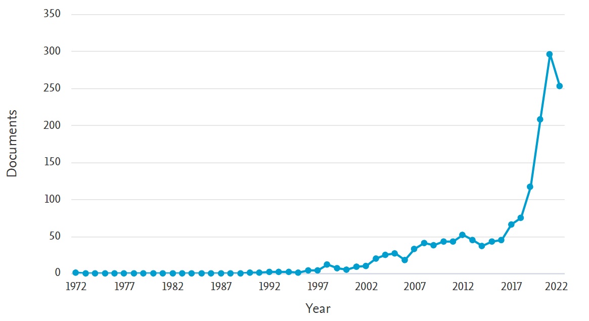
Figure 1. Number of publications that integrate AP and RL. This figure was obtained by introducing the following queries in Scopus (search performed on 9 December 2022): TITLE-ABS-KEY ( ( ”reinforcement learning” AND ”automated planning” ) OR ( ”model-based reinforcement learning” OR ”model-based RL” ) OR ( ”relational reinforcement learning” OR ”relational RL” ) OR ( ”automated planning” AND ( ”machine learning” OR ”deep learning” ) ) OR ( ”learn to plan” OR ”learning to plan” ) OR ( neurosymbolic OR neuro-symbolic OR neuralsymbolic OR neural-symbolic ) ) AND ( LIMIT-TO ( SUBJAREA , ”COMP” ) OR LIMIT-TO ( SUBJAREA , ”MATH” ) OR LIMIT-TO ( SUBJAREA , ”ENGI” ) ) AND ( EXCLUDE ( PUBYEAR , 2023 ) ) .

There exist many examples in the literature that study the application of AI to the problem of SDM from different perspectives. (Ghallab et al.,, 2016) summarizes the field of AP whereas (Sutton and Barto,, 2018) does the same for the field of RL and (Li,, 2018) overviews the subfield of DRL. Some works focus on the application of ML methods to the field of AP. (Jiménez et al.,, 2012) presents a review of ML methods for learning planning domains and search control knowledge, e.g., planning policies and heuristics. (Arora et al.,, 2018) focuses solely on ML techniques for learning planning domains. Other works survey RL methods which incorporate some characteristics of AP. (Moerland et al.,, 2023) presents a review of model-based RL, i.e., RL techniques which harness a model of the environment, and (Tadepalli et al.,, 2004) reviews the field of relational RL, i.e., RL methods which encode their knowledge in a symbolic way. Finally, some works focus on the actual integration of AP and RL. (Partalas et al.,, 2008) surveys methods which combine RL and AP to solve SDPs, but does not cover methods for learning the structure of SDPs such as the action model. (Moerland et al.,, 2020) presents a framework which unifies RL and AP approaches to solve SDPs. However, as the authors explicitly state, their work leaves out AP techniques which employ a symbolic knowledge representation, i.e., SP methods.

The main contribution of this work is to provide a review of symbolic, subsymbolic and hybrid AI methods for SDM. We propose a novel taxonomy which classifies these techniques according to their purpose, i.e., methods which solve SDPs versus methods which learn the structure of SDPs (e.g., the action model used in AP). Although this connection has been recognized informally in a number of places, to the best of our knowledge this is the first review which tries to cover all these different approaches and applications as part of the same work. We intend this review as an opportunity for researchers from both the AP and RL communities to learn from each other, in an effort to unify both fields. Due to the broad scope of our work, we limit this review to discrete SDPs, which can be formulated as finite Markov Decision Processes (MDPs) (Sutton and Barto,, 2018) and Partially Observable Markov Decision Processes (POMDPs) (Lovejoy,, 1991), and leave out SDPs with continuous state and/or action spaces. Moreover, we do not focus on a specific approach or technique but rather present an overview of the most important methods present in the literature. Throughout this work we reference several reviews for those readers who would wish to deepen into a specific topic.

An additional contribution of this work is provided in Section 5. Here, we discuss what properties an ideal method for SDM should exhibit. Based on these properties, we then analyse the advantages and disadvantages of the existing techniques for solving SDPs. As a result of this analysis, we argue that an ideal method for SDM should unify the symbolic and subsymbolic paradigms represented by AP and RL, respectively, and that neurosymbolic AI is the current approach which most closely resembles this ideal integration, thus posing a very promising line of work.

This review is organized as follows. Section 2 presents a formal description of SDPs as (PO)MDPs, used throughout the rest of the review. Sections 3 and 4 provide the taxonomy of methods for SDM, the first focusing on methods for solving MDPs whereas the latter focuses on methods for learning the structure of MDPs. Section 5 discusses the characteristics of an ideal method for SDM, as mentioned above. Section 6 proposes several directions for future work, based on the integration of symbolic and subsymbolic AI for SDM. Finally, Section 7 presents the conclusions of our work.

2. Problem Formulation

In this work, we focus on SDPs with a finite number of states and actions (decisions) and where time is discrete, i.e., after the execution of an action the environment immediately transitions from time instant $t$ to $t+1$. For totally observable environments where the agent has access to full information about the current state, this type of SDPs are commonly described as a finite Markov Decision Process (MDP). However, there exist different alternative formulations for MDPs. In this work, we will use the one given by finite Stochastic Shortest-Path MDPs (SSP MDPs) (Kolobov,, 2012), as they provide a general MDP formulation which suits both AP and RL. An SSP MDP is constituted by the following elements:

• State space $S$, the finite set of states of the system. In some SSP MDPs, at the beginning of the task the agent always starts from a state $s$ randomly sampled from a set of initial states $S_{i}\subset S$. In other SSP MDPs, the agent may start from any state $s\in S$, i.e., $S_{i}=S$.

• Action space $A$, the finite set of actions the agent can execute. In some SSP MDPs, only a subset of applicable actions $App(s)\subset A$ are available to the agent at a given state $s$. In other SSP MDPs, the agent can execute every action at every state, i.e., $App(s)=A\ \forall s\in S$.

• Transition function $T:S\times A\times S\rightarrow[0,1]$. It describes the dynamics of the environment, by specifying the probability $T(s,a,s^{\prime})=P(s^{\prime}|s,a)$ of the environment (SSP MDP) transitioning into state $s^{\prime}$ after the agent executes an (applicable) action $a\in App(s)$ at the current state $s$. If given some state $s\in S$ and action $a\in App(s)$ the environment always transitions into the same state $s^{\prime}$ (i.e., $P(s^{\prime}|s,a)=1$ and $P(s^{\prime\prime}|s,a)=0\ \forall s^{\prime\prime}\neq s^{\prime}$), the MDP is said to be deterministic. Otherwise, it is stochastic.

• Cost function $C:S\times A\times S\rightarrow[0,\infty)$. It gives a finite strictly positive cost $C(s,a,s^{\prime})>0$ when the agent goes from state $s$ to $s^{\prime}$ by executing the (applicable) action $a$. Transitions from a goal state are the only ones with a cost of zero.

• Goal set $G\subseteq S$. It contains a finite set of goal states $s_{g}\in S$, one of which must be reached by the agent. For every goal state $s_{g}\in G$, action $a\in A$ and non-goal state $s\notin G$, the following conditions are met: $T(s_{g},a,s_{g})=1$, $T(s_{g},a,s)=0$, $C(s_{g},a,s_{g})=0$. Intuitively, these conditions mean that goal states are terminal, since once reached the agent cannot leave them and no longer incurs in additional costs.

A policy $\pi:S\times A\rightarrow[0,1]$ is a partial function which maps every state $s\in S$ to a probability distribution over applicable actions $a\in App(s)$. The solution of an SSP MDP is an optimal policy $\pi^{*}$, i.e., a policy which minimizes the expected cost needed to reach a goal state $s_{g}\in G$ from an initial state $s_{i}\in S_{i}$. A plan $p$ is the instantiation of a policy $\pi$ starting from an initial state $s_{0}\in S_{i}$, i.e., the sequence of states and actions $s_{0},a_{0},s_{1},a_{1},...,s_{n-1},a_{n-1},s_{n}$ which results from applying at each state $s_{j}$, where $0\leq j<n$, the action $a\in App(s_{j})$ selected by $\pi$. Given an initial state $s_{i}$, if both the policy $\pi$ and MDP are deterministic, the instantiation of $\pi$ from $s_{i}$ produces a single plan $p$. If either the policy or MDP are stochastic, the instantiation produces a (possibly infinite) set of plans.

We previously stated SSP MDPs are suitable for both AP and RL. However, in most RL tasks the goal is to find a policy $\pi^{*}$ which maximizes the sum of rewards $r$, instead of minimizing the cost needed to reach a goal state $s_{g}\in G$. In finite-horizon (FH) MDPs, the sum of rewards must be maximized over a finite number of time steps. In infinite-horizon (IFH) MDPs on the other hand, the goal is to maximize the sum of rewards, discounted by a factor $\gamma$, over an infinite number of time steps. It can be proven that both types of reward-based MDPs, FH and IFH MDPs, can be expressed as an equivalent SSP MDP, in terms of goals and costs instead of rewards (Kolobov,, 2012). Therefore, the reward-based MDPs usually employed in RL are merely subclasses of the more general SSP MDPs. For this reason, in this work we will interchangeably employ the reward-based formulation of RL and the goal-based formulation of AP, knowing that both of them can be expressed as SSP MDPs.

Finally, all types of MDPs exhibit a very important feature, known as the Markov property. This property states that, in any MDP, the cost $C$ (or reward $R$) and transition function $T$ only depend on the current state $s$ of the MDP and the action $a$ executed by the agent at that state. This property allows agents to select actions by only considering the information about their current state and not their past history, i.e., past states and actions. If the environment is partially observable, i.e., the agent lacks information about the current state, the SDP must be described as a POMDP (Lovejoy,, 1991). POMDPs share the same formulation as (totally observable) MDPs and also follow the Markov property. However, the current state of POMDPs is hidden and the agent only receives partial information in the form of observations about the state. These observations must then be used by the agent to infer the actual state of the environment and solve the POMDP.

3. Methods to Solve MDPs

In this section we present an overview of the main methods to solve MDPs (see Figure 2). Historically, there exist two main competing approaches for finding this solution. AP (Ghallab et al.,, 2016) proposes a synthesis-based paradigm, in which the prior information about the MDP is used to carry out a search and reasoning process in order to find its solution. RL (Sutton and Barto,, 2018), on the other hand, presents a learning-based approach inspired by ML, where the agent does not synthesize the solution of the MDP but rather learns it automatically from data. In this work, we also discuss a novel family of methods which can be considered as a sub-category of both AP and RL, as they integrate both approaches. This group is composed of methods which learn to plan (Moerland et al.,, 2023). In the same manner as AP, these methods carry out a planning process to find the solution of the MDP. However, unlike them, they learn how to actually perform the planning computations automatically from data, similarly to how RL techniques learn the optimal policy from data.

Figure 2. Diagram of methods to solve MDPs.

3.1. Automated Planning

AP (Ghallab et al.,, 2016) is a subfield of AI which provides a set of deliberative techniques to solve MDPs. AP methods harness the information about the environment dynamics to synthesize the solution of the MDP. This information is encoded in the action model, sometimes also referred to as the planning domain, which represents the available actions for the agent and how they affect the current state of the world. The solution of the MDP is often formulated as the policy or plan that achieves a set of goals while minimizing the cost needed to obtain them. In other cases, it is formulated as the policy that maximizes a reward function. AP methods can be split in two main categories according to the type of knowledge representation employed: SP and NSP.

3.1.1. Symbolic Planning

We use the name SP to refer to those AP techniques which require a symbolic description of the MDP. SP makes use of a formal language based on FOL, such as PDDL (Younes and Littman,, 2004) and RDDL (Sanner et al.,, 2010), to encode the information about the planning task to solve. This information is split in two different items: a domain and a problem. The domain encodes the MDP dynamics whereas the problem encodes the initial state and goal to achieve. This allows for great reusability, since different MDPs which share the same dynamics can be described with the same domain. Another advantage of using logic-based languages to represent MDPs is that planners can exploit this description to speed up planning (see Section 3.1.3). The simplest and best studied case of SP is Classical Planning (CP) (Ghallab et al.,, 2016), sometimes also called STRIPS-based planning. CP addresses MDPs that meet a series of characteristics: the MDP contains a finite number of states; it is fully observable (not a POMDP); it is deterministic; there are no exogenous events (every change in the world is directly produced by the agent); the objective of the agent is to attain a series of goals; the solution of the MDP is expressed as a plan; time is implicit, i.e., actions are assumed to be executed instantly; and, lastly, planning is performed offline. An example CP task is shown in Figure 3. CP methods are often classified according to the cost guarantees they provide into three different groups: optimal, satisficing and agile. Optimal planners always find the optimal solution of the MDP, i.e., the plan of minimum cost, assuming such a plan exists. In case all actions have the same cost, this corresponds to the shortest plan. Satisficing planners, on the other hand, try to minimize plan cost but do not guarantee finding the optimal plan, as they try to maintain a balance between plan quality and planning time. Finally, agile planners completely disregard plan cost and only focus on finding a valid plan as quickly as possible.

There exist many different methods that address CP, such as FastForward (FF) (Hoffmann,, 2001), FastDownward (FD) (Helmert,, 2006), LAMA (Richter and Westphal,, 2010) and Dual-BFWS (Frances et al.,, 2018), just to cite a few. These planners mainly differ in the search algorithm employed and the information used to guide the search (see Section 3.1.3). Nowadays, most state-of-the-art planners also support many extensions to CP, e.g., action costs, negative preconditions, and conditional effects (Haslum et al.,, 2019). Nonetheless, there also exist other CP extensions for which the support is more limited. Some examples are: Temporal Planning (Fox and Long,, 2003), where planners need to reason about durative actions, parallel execution, deadline goals and other temporal aspects; Generalized Planning (Jiménez et al.,, 2019), where the goal is to obtain plans which solve a set of problems instead of a single one; Mixed-Initiative Planning (Burstein and McDermott,, 1996), which comprises systems that support human-machine collaboration for plan generation and management; planning in non-deterministic MDPs, covered by the subfields of Probabilistic Planning (Younes and Littman,, 2004) and FOND Planning (Cimatti et al.,, 2003); and planning in POMDPs, covered by Contingent Planning (Draper et al.,, 1994) (when both the initial and run-time states can be observed) and Conformant Planning (Goldman and Boddy,, 1996) (when only the initial state can be observed).

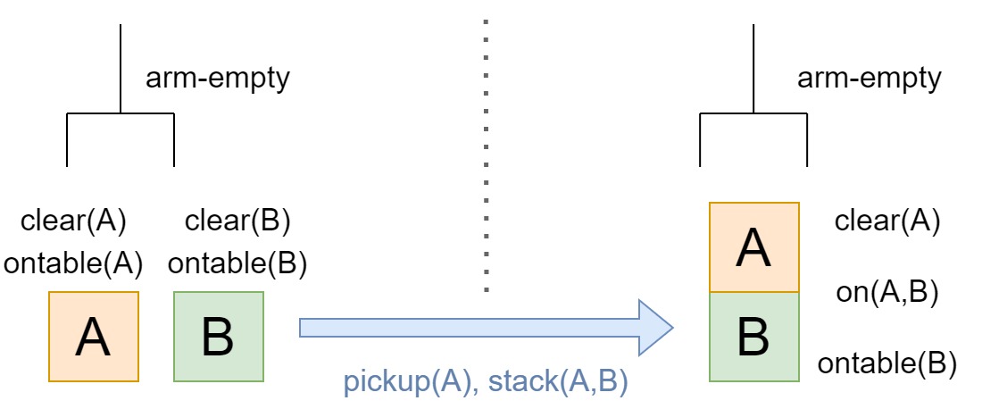
Figure 3. Example of a CP task. The task belongs to the CP domain known as blocksworld, consisting of blocks that can be stacked one upon another with a gripper arm. The blue arrow represents a plan that achieves the goal state (right) starting from the initial state (left).

3.1.2. Subsymbolic Planning

We use the name NSP to refer to those AP methods which do not require a symbolic description of the MDP. NSP methods only need as action model a transition function that maps a state-action $(s,a)$ pair into its corresponding next state $s^{\prime}$ and do not care about how such function is implemented. This makes possible to apply NSP to situations where the environment dynamics are known but are not given in a formal, logic-based description. Due to this, most model-based RL techniques employ this type of planning. Nevertheless, this simplicity of representation also has its downsides. Whereas SP methods are able to exploit a rich relational description of the MDP to improve the search process, e.g., by the use of powerful delete-relaxation heuristics (see Section 3.1.3), NSP techniques must resort to other methods.

NSP can be roughly reduced to two main aspects: how the state space is explored and how the solution is represented. Regarding the solution representation, some search algorithms like A* (Ferguson et al.,, 2005) try to find the minimum-cost plan from the initial state to a goal state. Other algorithms like Policy Iteration (Sutton and Barto,, 2018) explore the reward obtained by different state-action sequences in order to find the policy which maximizes reward. In order to explore the state space, many different strategies have been proposed. Some methods like depth-first search (Tarjan,, 1972) only explore a single trace at a time while others like breadth-first search (Bundy and Wallen,, 1984) maintain a list of open states which can be selected for the next exploration step. In some situations, we have access to a domain-specific heuristic that we can exploit to direct the search process, using best-first search algorithms like A* (Ferguson et al.,, 2005). In other cases, such heuristic is unavailable, so a different method must be employed. Some algorithms explore the state space in order to learn search control knowledge. MonteCarlo Tree Search (MCTS) (Browne et al.,, 2012) is a good example of this. It performs rollouts, i.e., simulations, to estimate the value of a given state (see Figure 4) and uses the UCB1 (Auer et al.,, 2002) method to balance the exploitation of promising states with the exploration of less visited states. As an alternative approach, (Frances et al.,, 2017) shows that it is possible to compute domain-independent planning heuristics, like those obtained by SP techniques, with a subsymbolic (i.e., black-box) action model, although a symbolic description of states and actions is still needed. More information about NSP methods and their relation with RL can be found in (Moerland et al.,, 2020).

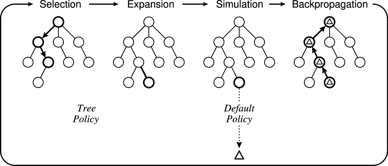
Figure 4. One iteration of MCTS (Browne et al.,, 2012). In the Selection Phase, the tree policy is used to traverse the tree and select a promising node. Then, a child of the node is added to the tree (Expansion Phase). Next, in the Simulation Phase, the new node is evaluated by selecting actions according to the default policy. Finally, the simulation result is backed up the tree to update the node evaluations (Backpropagation Phase).

It is important to note that NSP methods can be used in conjunction with symbolic representations. Therefore, the difference between SP and NSP is that, while SP methods require a symbolic description of the MDP, in the case of NSP methods this is optional. For example, both the MCTS and A* algorithms can be applied to MDPs encoded in FOL, as (Trunda and Barták,, 2013) and (Hoffmann,, 2001) respectively show. At the same time, they can also be applied to MDPs represented subsymbolically. A* can be used as long as a suitable heuristic is provided (e.g., the Manhattan distance for pathfinding problems) and MCTS only needs to perform rollouts in order to estimate the state value needed to guide the search.

3.1.3. Planning policies and heuristics

Planning is computationally expensive. Even for the simplest case, CP, it is known to be PSPACE-complete (Bylander,, 1994). For this reason, if we hope to apply AP methods to solve real problems we need to harness control knowledge to direct the search towards promising regions of the state space. This knowledge can come in two main ways: planning policies and planning heuristics. A planning policy is a function which maps a planning context, consisting of information about the current state and goals to achieve, to the best actions to execute in that context. A planning heuristic predicts the distance (cost) from the current state to a goal state. It implicitly defines the best action to apply, i.e., the one with the minimum predicted heuristic value. Planning policies and heuristics are analogous to goal-conditioned/generalized policies and value functions in RL (Schaul et al.,, 2015), which generalize RL policies/value functions to solve several tasks instead of just one.

Control knowledge can be designed to be domain-independent or be tailored to a specific planning domain. The first option is the most widely used among SP methods. These techniques exploit the rich symbolic representation of the MDP to implement powerful domain-independent planning heuristics, which can be applied to any planning domain. One of the most popular approaches are the so-called delete-relaxation heuristics (Keyder et al.,, 2014), which estimate the distance from the current state to the goal in a simplified version of the planning task where the delete effects of actions are ignored. As an alternative approach, some methods use some sort of domain-specific knowledge which makes possible to obtain quality solutions for a specific planning domain in a very efficient way. For instance, the L1 norm or Manhattan distance provides a straightforward heuristic which has been applied to many pathfinding problems (Silver,, 2005; Botea et al.,, 2013). However, in some situations we may not have access to this type of prior information. For these cases, there exist many methods to learn control knowledge from example plan traces. The problem of learning planning heuristics corresponds to a regression task, which can be solved with different ML methods, e.g., linear regression (Yoon et al.,, 2006), regression trees and support vector machines (ús Virseda et al.,, 2013). Neurosymbolic methods have also been employed for learning heuristics. (Shen et al.,, 2020) applies Graph Neural Networks (GNNs) (Battaglia et al.,, 2018) to predict the heuristic value from the delete-relaxation representation of the problem, whereas (Gehring et al.,, 2022) leverages domain-independent SP heuristics to efficiently learn domain-specific heuristics with DRL. There exist two main approaches for learning planning policies. The first one is to represent the policy as a set of rules, which are learned with some algorithm (Leckie and Zukerman,, 1998; Aler et al.,, 2002). The second option is to use Case-Based Reasoning and represent the policy as a library of solutions (plans) to problems and a distance metric to retrieve similar instances (Veloso and Carbonell,, 1993; Serina,, 2010). A more comprehensive review of methods to learn search control knowledge can be found in (Jiménez et al.,, 2012).

3.2. Reinforcement Learning

RL (Sutton and Barto,, 2018) is a subfield of ML that provides an alternative approach to AP for solving MDPs. Instead of employing an action model to synthesize the solution of the MDP, RL techniques use the data gathered from the environment to learn the optimal policy that maximizes reward. To do so, they must balance the exploration of the environment, i.e., the process of trying out new actions and observing their outcomes, with the exploitation of the learned knowledge, i.e., selecting the best action found so far (which might not be the optimal one). This is known as the exploration-exploitation tradeoff. Most RL methods, known as model-free RL, do not need a model of the environment to learn the optimal policy. However, some methods known as model-based RL harness the information contained in the action model to facilitate the learning process. In addition, although the vast majority of RL techniques represent the information in a subsymbolic way, some of them known as relational RL (Tadepalli et al.,, 2004) use a symbolic knowledge representation analogous to that of SP.

3.2.1. Model-free RL

Model-free RL provides methods to learn the optimal policy when the model of the world, i.e., the action model, is unknown. These methods can be further grouped in (model-free) value-based and policy-based RL. Value-based RL learns to estimate the expected cumulative reward $\mathbb{E}_{\pi^{*}}[R]$, referred to as the return, associated with a state (value function $V(s)$) or a state-action pair (action-value function $Q(s,a)$). Once this function has been learned, the optimal policy simply corresponds to selecting in each state the action with the maximum return. A classical algorithm for value-based RL is Q-Learning (Watkins,, 1989). Q-Learning utilizes the Bellman optimality equation to learn the optimal Q-value $Q(s,a)$ associated with each state-action pair $(s,a)$, i.e., the maximum return that can be obtained for each $(s,a)$ pair. These Q-values need to be stored for every possible combination of states and actions, which results infeasible for MDPs with large state spaces. Deep Q-Learning (Mnih et al.,, 2013) solves this problem by making use of a DNN which is used to approximate the Q-values. Since this DNN is capable of generalizing to new states, it does not need to memorize the $Q(s,a)$ value for every $(s,a)$ pair, thus making it possible to apply this algorithm to real-world problems with large state spaces.

In contrast to value-based methods, policy-based RL explicitly learns the optimal policy without needing to estimate the return $V(s)$ or $Q(s,a)$. One of the most well-known algorithms in this category is REINFORCE (Williams,, 1992). REINFORCE uses a DNN to approximate the policy, i.e., given an input state it returns a probability distribution over the actions. This DNN is then trained using gradient-based methods to maximize the probability of selecting actions with a large return $Q(s,a)$ associated. One main issue of REINFORCE is that $Q(s,a)$ is not always a good measure of action optimality, since it does not only depend on the action $a$ but also on the state $s$ the action is executed. Advantage Actor Critic (A2C) (Mnih et al.,, 2016) tries to solve this problem by substituting $Q(s,a)$ for the advantage $A(s,a)=Q(s,a)-V(s)$, which measures how good $a$ is when compared to the average action at $s$. A2C trains two separate DNNs: the actor and the critic. The critic learns to predict the return $V(s)$ of a given state, which is then used to calculate $A(s,a)$. The actor learns the optimal policy by using the same method as REINFORCE. However, it utilizes the advantage $A(s,a)$ predicted by the critic to measure action optimality, instead of $Q(s,a)$. Thus, A2C entails a hybrid approach which integrates both value and policy-based RL. A deeper view into classical RL and DRL methods can be found in (Sutton and Barto,, 2018) and (Li,, 2018), respectively.

3.2.2. Model-based RL

Model-based RL tries to combine the fields of RL and AP. It enhances standard, model-free RL algorithms with a model of the world, which can be employed in two main ways. The first alternative is to use the action model as a simulator to obtain data for training the policy, thus minimizing the required amount of interaction with the real world. For this reason, model-based RL techniques are more sample-efficient, i.e., need less data to learn the optimal policy, than model-free methods (Kaiser et al.,, 2019). A second alternative is to integrate a deliberative process into the decision-making cycle of RL. Instead of simply selecting the best action according to the policy, we can use the action model to carry out a planning process, guided by the learned policy/value function, in order to select the next action to execute. This approach blurs the line between model-based RL and AP with a learned heuristic. Finally, we can differentiate between model-based RL methods which require the action model is given a priori and those which do not. This second category of methods use the data collected from the environment to learn the action model in addition to a policy, employing some of the techniques commented in Section 4.1.

We will use Dyna (Sutton,, 1991) and AlphaZero (Silver et al.,, 2018) as illustrative examples of the different existing model-based RL algorithms. One of the oldest examples of model-based RL can be found in Dyna. This method learns a subsymbolic, black-box model of the world. Then, it trains the Q-Learning algorithm on both experience obtained from the real world and data sampled using the learned action model. Dyna performs reactive execution, i.e., the action to execute is selected according to the value function trained with Q-Learning, with no planning involved whatsoever. AlphaZero is a novel model-based RL method which has been successfully applied to play the games of chess, shogi and Go at superhuman level. Unlike Dyna, it requires a prior model of the world, although a newer version of this model known as MuZero (Schrittwieser et al.,, 2020) overcomes this limitation. AlphaZero trains both a value function and a policy, implemented as a single Deep CNN (Krizhevsky et al.,, 2012), which together guide the planning process performed by the MCTS algorithm. This planning process outputs a probability distribution from which the action to execute is sampled. The value function is trained to predict the game winner from the current state whereas the policy is trained to match the probabilities obtained by MCTS. Thus, in AlphaZero there exists a clear synergy between RL and AP: RL is used as a heuristic to guide the planning process, which in return allows to obtain data to train the RL policy, acting as a policy improvement operator. A comparison between AlphaZero and the model-free RL algorithm Deep Q-Learning is shown in Figure 5. Finally, a more comprehensive review of model-based RL is provided in (Moerland et al.,, 2023).

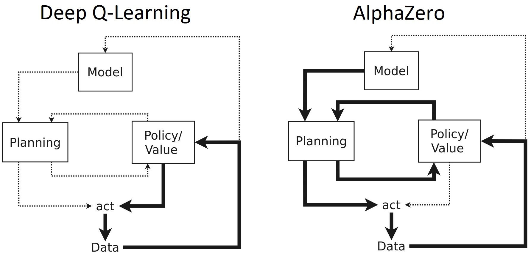
Figure 5. Model-free vs model-based RL (adapted from (Moerland et al.,, 2023)). Figure compares the architectures of a model-free RL algorithm (Deep Q-Learning) and a model-based RL method (AlphaZero). Thick lines are used by the algorithm whereas dotted lines are not, and are displayed just for comparative purposes. It can be observed that Deep Q-Learning does not use an action model or perform any planning whatsoever. Conversely, AlphaZero uses an action model (given a priori) to perform a planning process (guided by a policy and value function) that selects the next action to execute.

3.2.3. Relational RL

Relational Reinforcement Learning (RRL) (Tadepalli et al.,, 2004) can be considered the intersection of RL and Relational Learning (Koller et al.,, 2007). It is comprised of methods that combine RL with the symbolic representations employed in SP. These symbolic representations are well suited for MDPs that can be naturally described in terms of objects and their interactions, known as object-oriented MDPs (Diuk et al.,, 2008). RRL methods leverage lifted representations, i.e., symbolic representations with variables, to abstract from concrete objects and, thus, naturally generalize to tasks with varying number of objects. In addition, the knowledge learned by RRL techniques is more amenable to interpretation than the one typically learned in DRL.

One of the best known RRL algorithms is relational Q-Learning (Džeroski et al.,, 2001). This method utilizes a symbolic knowledge representation for the goal-conditioned action-value function $Q(s,a,g)$. This function is learned with a relational regression tree (Kramer,, 1996) which, given the current state $s$, goal $g$ to achieve and action $a$ to execute, predicts the associated Q-value $Q(s,a,g)$ (see Figure 6). The relational P-function (Džeroski et al.,, 2001) is a form of policy-based RRL which explicitly encodes the policy represented by the relational Q-function. It also uses a relational tree but, instead of returning $Q(s,a,g)$, it outputs whether $a$ is optimal given $s$ and $g$. (Boutilier et al.,, 2001) is an example of model-based RRL. It proposes a symbolic dynamic programming method which adapts the algorithm known as Value Iteration (Sutton and Barto,, 2018) to the relational setting. In recent years, there has been a renewed interest in RRL. (Yang et al.,, 2018) proposes PEORL, a model-based RL architecture which combines SP and Hierarchical RL. It utilizes a symbolic action model (given a priori) to generate plans that guide the RL algorithm, and leverages the learned experience to enrich the symbolic knowledge and improve planning. On the other hand, (Zambaldi et al.,, 2018) proposes a Deep RRL algorithm that departs from the classical RRL definition, since it does not use a symbolic representation. Instead, the authors opt for a deep attention-based model (Vaswani et al.,, 2017) which improves the efficiency, generalization capacity and interpretability of conventional DRL. It detects the objects of the scene with a CNN and reasons about their interactions with a self-attention mechanism, composed of blocks that can be stacked together to infer higher-order relations between objects.

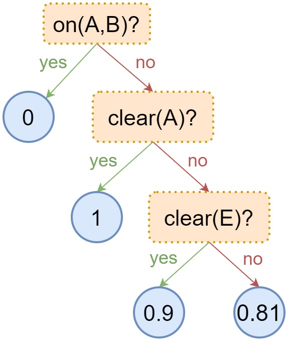
Figure 6. Regression tree learned with relational Q-Learning (adapted from (Džeroski et al.,, 2001)). The example corresponds to the blocksworld domain (see Figure 3). The tree encodes the $Q(s,a,g)$ value for the goal $g=on(A,B)$ and action $a=stack(D,E)$. Inner nodes (orange) check the truth value of a grounded predicate of the state $s$, whereas leaf nodes (blue) return the corresponding Q-value.

3.3. Learn to plan

As we have seen previously, many MDP-solving techniques make use of an action model, which can be either known or learned from data. This model of the world can be used in several ways. The first option is to plan over it. We can use a symbolic planner, e.g., FastForward (Hoffmann,, 2001), or a NSP procedure, e.g., MCTS (Browne et al.,, 2012), depending on the type of knowledge representation used by the model, in order to simulate different courses of action and find the best one. The second option is to leverage the action model to obtain a policy or value function/heuristic. We can follow the model-based RL approach and employ the model to obtain data for training a value function or policy, or do as in SP and compute a domain-independent heuristic using the planning domain and problem. In addition to these two options, there exists a third alternative which has not been discussed yet: to learn to plan (Moerland et al.,, 2023). This idea combines the RL and AP approaches and is inspired by the novel area of algorithmic reasoning (Cappart et al.,, 2021), which studies how to teach DNNs to compute algorithms. In the case of SDM, instead of considering the planning procedure as an external process, we can integrate it into the computational graph of our DNN, i.e., the graph containing the sequence of operations performed by the model to transform the inputs into outputs. There exist three main ways to embed the planning procedure into a DNN. Firstly, we can learn an action model that is compatible with a planning algorithm chosen a priori. Secondly, given an action model, we can learn how to perform the actual planning computations on it. Finally, we can jointly learn the action model and planning algorithm at the same time.

3.3.1. Fix the planning algorithm and learn the action model

Some methods choose a planning algorithm a priori and embed it into the computational graph of the decision-making model. If the planning procedure is differentiable, it is possible to learn an action model compatible with it by using gradient-based optimization techniques. The action model is trained to output the optimal policy or value function as a result of the iterative computations performed by the chosen planning algorithm. Therefore, the action model learns a representation of the dynamics tailored to the task at hand and the specific planning algorithm employed, as opposed to most action models which represent the environment dynamics in a general, task-independent way. This special type of action models belong to the family of value-equivalent action models (see Section 4.1.2).

Value Iteration Networks (VINs) (Tamar et al.,, 2016) are a good example of this. The authors of this work propose a differentiable implementation of the classical Value Iteration algorithm using recurrent CNNs (see Figure 7). This planning procedure is then embedded into a DNN architecture which can be trained end-to-end to predict the optimal policy by using standard RL and Supervised Learning (SL), i.e., ML methods which are trained on labeled samples corresponding to (input, output) pairs. The obtained model generalizes better than reactive policies, i.e., those that do not perform planning, when applied to new problems of the same domain. Universal Planning Networks (UPNs) (Srinivas et al.,, 2018) follow a similar approach. This work proposes a DNN architecture which learns a policy for a continuous task. The architecture integrates a differentiable planning module, which performs planning by gradient descent, and is trained end-to-end with SL to predict the optimal policy. The resulting action model exhibits a state representation suitable for gradient descent planning, which can be adapted to other tasks.

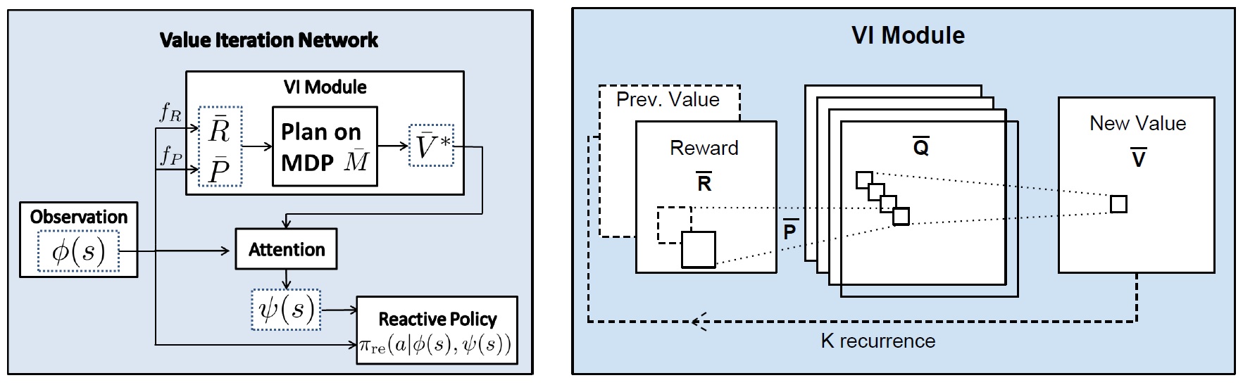
Figure 7. Value Iteration Network (VIN) (Tamar et al.,, 2016). Picture on the left shows the global VIN architecture, which receives as input a state observation $\phi(s)$ and outputs the policy $\pi_{re}$. Picture on the right shows the Value Iteration module, a recurrent CNN that performs the computations of the Value Iteration algorithm.

These methods are similar to those discussed in Section 4.1.2 like MuZero, since they also learn a value-equivalent action model that is suitable for planning. The difference between both types of methods is how the planning process is implemented. In MuZero, planning is performed explicitly, outside the computational graph. It learns a state representation useful for predicting the rewards, value function and policy for any given state. In VINs and UPNs, however, planning is performed implicitly, as a differentiable process embedded into the computational graph to predict the optimal policy. Thus, they may learn a slightly different state representation to that employed by MuZero and other models where planning is performed as a separate process.

3.3.2. Fix the action model and learn the planning algorithm

Other methods follow the opposite approach. Given an action model, which can be either known a priori or learned as a first step, they learn how to plan over it in order to solve the corresponding SDM task. The planning algorithm obtained will be able to harness the information contained in the action model to predict the optimal policy or value function. The existing methods in the literature provide different amounts of freedom to the planning algorithm, by controlling which parts of it are fixed a priori and which ones must be learned.

(Guez et al.,, 2018) proposes MCTSnet, a DNN architecture that embeds the MCTS algorithm into its computational graph. This model learns how to perform the different MCTS operations (selection, expansion, simulation and backpropagation) in order to play the Sokoban game. Other works give even more freedom to the planning process. (Pascanu et al.,, 2017) proposes Imagination-Based Planner (IBP), a DNN architecture capable of constructing, evaluating and executing plans. It learns when to plan, which states to expand and when to stop planning. Both MCTSnet and IBP utilize a subsymbolic representation for their learned knowledge. Instead, (Toyer et al.,, 2018) proposes Action Schema Networks (ASNets), a neurosymbolic model for learning to plan. ASNets correspond to DNNs specialized to the structure of planning problems (see Figure 8). They are composed of alternating action and proposition layers, with the specific network topology given by the associated planning domain and problem to solve, and a final layer which outputs the policy. Policies learned by ASNets are shown to generalize to different problems of the same domain.

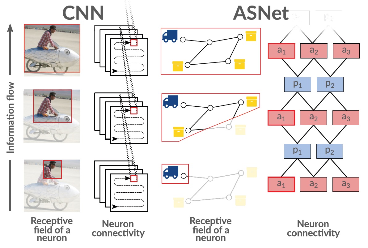
Figure 8. Comparison between ASNets and CNNs (Toyer et al.,, 2018). In a CNN, successive convolutions grow the receptive field of a neuron at higher layers; analogously for ASNet, a neuron for a particular action $a$ or proposition $p$ sees a larger portion of the current state at higher layers.

3.3.3. Learn both the action model and planning algorithm

Lastly, some methods combine the two previous approaches. They embed a differentiable action model and differentiable planning procedure into the same computational graph, and then jointly optimize both parts to solve a particular SDM task. Although this idea represents the most end-to-end approach for learning to plan, the resulting model is hard to optimize, due to its great complexity and the interdependence between the action model and planning algorithm, as the quality of one depends on the quality of the other and vice versa.

In (Farquhar et al.,, 2018), RL is used to jointly learn an action model and how to plan over it. The proposed method, called TreeQN, employs the learned model to try all possible action sequences up to a predefined depth, learning to predict the state values and rewards along the simulated trajectories. These values are then backed up the search tree to estimate the Q-values at the current state. (Guez et al.,, 2019) proposes the Deep Repeated ConvLSTM (DRC) model, a powerful DNN architecture capable of learning to plan even though it incorporates no inductive bias for that purpose beyond its iterative nature. The model is composed of stacked ConvLSTM (Shi et al.,, 2015) blocks which are repeatedly unrolled to predict the policy and value function. The authors show that DRC exhibits characteristics of planning, such as an increase in performance when given additional thinking time.

4. Methods to Learn the Structure of MDPs

Every MDP has a different underlying structure. Its most important features are encoded in the action model, which describes the environment dynamics and is required by many of the MDP-solving methods seen in the previous section, e.g., AP and model-based RL. In addition to the action model, there exist specific aspects of the MDP structure, e.g., landmarks (Hoffmann et al.,, 2004) and state invariants (Fox and Long,, 1998), which if known can facilitate its resolution and also provide insight into the properties of the MDP. On top of that, some learning methods (Shen et al.,, 2020; Balduccini,, 2011; Hogg et al.,, 2008) require training data in the form of problem instances and plan traces, which often need to be provided by domain experts. In this section, we discuss the main methods (see Figure 9) for learning these different aspects of the MDP structure in case they are not given a priori.

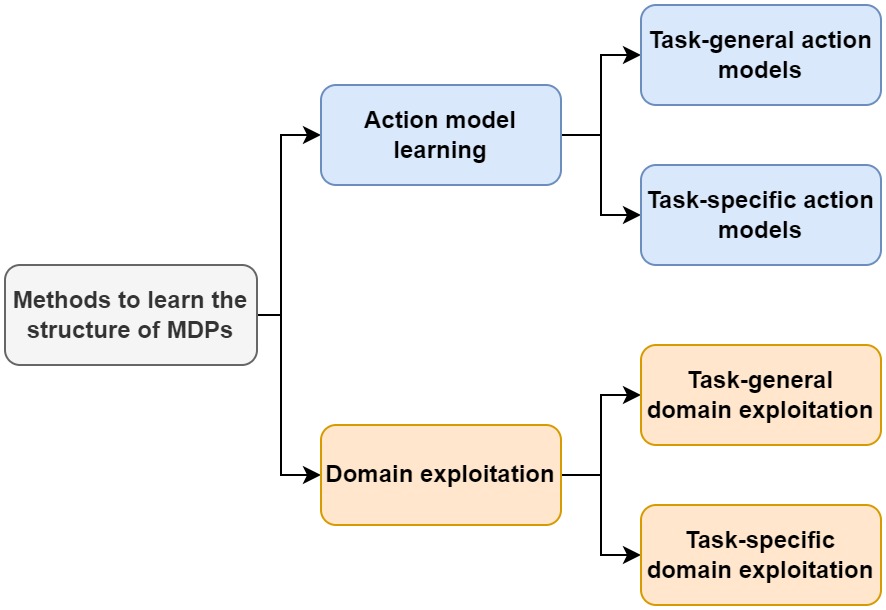
Figure 9. Diagram of methods to learn the structure of MDPs.

4.1. Action model learning

The action model, which also receives the names of planning domain and world model, represents the most important aspect of the MDP structure. It encodes the dynamics of the environment and how the agent can affect them, i.e., the available actions for the agent and the effect each action has on the world state. The action model is essential for AP techniques, which need it to carry out their deliberative process. It also results advantageous for RL as it has been shown that those techniques which use an action model, i.e., model-based RL, are more sample-efficient than those which do not, i.e., model-free RL (Kaiser et al.,, 2019). Here, we discuss methods for automatically learning the action model from data. These techniques can be categorized according to the scope of the learned model in methods which learn task-general action models and those which learn task-specific action models.

4.1.1. Task-general action models

These methods try to learn a model which represents the dynamics of the environment as accurately as possible, in what is known as a task-general action model. Instead of learning a model tailored for a specific task/problem, i.e., a specific reward function in RL or a particular set of goals in AP, they obtain a general model which can, in theory, be applied to solve any task of the corresponding domain. These techniques can be further grouped according to the type of knowledge representation employed by the learned model.

Task-general models with subsymbolic knowledge representation. These models represent the environment dynamics in a subsymbolic way, often as a black-box which receives as inputs a state $s$ of the world and an action $a$ to execute, and outputs the next state $s^{\prime}$ and often also the associated reward $r$ (see Figure 10, right). They are usually trained with ML and DL techniques, e.g., linear regression (Sutton et al.,, 2008), nearest neighbours (Jong and Stone,, 2007), random forests (Hester and Stone,, 2013), gaussian processes (Wang et al.,, 2005) and DNNs (Wahlström et al.,, 2015), in a supervised manner on samples of the form $(s,a,r,s^{\prime})$ collected from the environment.

For an effective learning of subsymbolic action models, some aspects which contribute to the uncertainty of the model must be considered. Firstly, we need to take into account the estimation errors which occur when the model is applied to regions of the state-space not seen during training. Most works, such as PILCO (Deisenroth and Rasmussen,, 2011), address this problem by estimating the uncertainty in the model predictions. Secondly, most environments are non-deterministic, so the learned action model must reflect this stochasticity in some way. Two possible solutions are to approximate the entire next state distribution (Khansari-Zadeh and Billard,, 2011) and to learn a generative model from which we can draw samples (Depeweg et al.,, 2017). Thirdly, some environments exhibit partial observability, i.e., they are POMDPs. Action models for POMDPs need to incorporate information about previous states using methods such as belief states (Chrisman,, 1992), recurrent neural networks (Chiappa et al.,, 2017) or neural turing machines (Gemici et al.,, 2017). Finally, in order to perform a multi-step look-ahead, the predicted next state $s^{\prime}$ must be repeatedly fed into the model as input. To prevent prediction errors from accumulating, some works use multi-step prediction losses for training (Abbeel and Ng,, 2005) whereas others learn different models for each n-step prediction (Asadi et al.,, 2018). A deeper view into subsymbolic action models can be found in (Moerland et al.,, 2023).

Task-general models with symbolic knowledge representation. These models use an interpretable, formal language based on FOL to represent objects, i.e., constants, and their relations, i.e., predicates. One example is PDDL (Haslum et al.,, 2019), the standard language in AP for representing planning domains (action models) and used by the majority of automated planners. In PDDL, the planning domain encodes the existing types of objects, predicates and actions. Each action has a series of parameters (variables that can be instantiated with objects), preconditions (predicates which must be true or false before executing the action) and effects (see Figure 10, left). The effects correspond to those grounded predicates (i.e., atoms) which, after applying the action to the current state, will become true (add effects) and those which will turn false (delete effects).

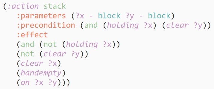
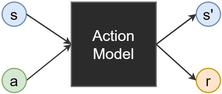
Figure 10. Symbolic and subsymbolic action models. Left: extract from symbolic action model, corresponding to the PDDL description of action stack in the blocksworld domain. Given a symbolic description of a state $s$, as a set of objects and atoms, and a grounded applicable action $a$, i.e., an action with parameters instantiated on objects at $s$ and whose preconditions are met at $s$, it allows to obtain the next state $s^{\prime}$ by applying the effects of $a$ to $s$. Right: subsymbolic action model, corresponding to a black-box. It receives a subsymbolic representation of $s$ (e.g., as an image or a set of state variables) and $a$ as inputs, and outputs $s^{\prime}$ and $r$. The symbolic action model is amenable to interpretation, whereas the subsymbolic one is usually not.

Methods for learning symbolic action models usually receive as input a set of plan traces, i.e., sequences of interleaved states and actions $(s_{0},a_{0},s_{1},...,a_{n-1},s_{n})$, obtained by solving planning problems of the corresponding domain. Then, they try to find the planning domain, i.e., the preconditions and effects of each action in the domain, which best fits the plan traces. The simplest scenario corresponds to learning planning domains for totally-observable, deterministic environments. This is a well-studied problem which has been solved in numerous ways (Shen and Simon,, 1989; Gil,, 1992; Wang,, 1996; Walsh and Littman,, 2008). Action preconditions are inferred by analysing the predicates which appear at the states preceding an action whereas action effects are learned by comparing the predicates of the states before and after applying the action, in what is known as the delta-state. Other works learn planning domains for environments with uncertainty, which can come in the form of non-deterministic actions or partial observability of states (POMDPs). (Oates and Cohen,, 1996; Pasula et al.,, 2007; Jiménez et al.,, 2008) tackle the case of non-determinism whereas (Yang et al.,, 2007; Zhuo and Yang,, 2014; Mourao et al.,, 2008) do the same for partially observable environments. (Segura-Muros et al.,, 2021) also tackles partially observable environments but is able to learn more expressive domains than the previous methods, with numerical variables and relations. The hardest case corresponds to learning action models for environments which present both non-determinism and partial observability. This problem has been poorly studied, with just one preliminar work trying to address it (Yoon and Kambhampati,, 2007). Finally, we can classify the existing methods according to the type of algorithm used to learn the planning domain, e.g., RL (Safaei and Ghassem-Sani,, 2007), relational RL (Rodrigues et al.,, 2011), surprised-based learning (Molineaux and Aha,, 2014), SL (Mourao et al.,, 2008), inductive rule learning (Segura-Muros et al.,, 2021), MAX-SAT (Yang et al.,, 2007) and transfer learning (Zhuo and Yang,, 2014). A deeper view into symbolic action models can be found in (Jiménez et al.,, 2012; Arora et al.,, 2018).

Task-general models with hybrid knowledge representation. Several works use a hybrid knowledge representation for the action model, one that sits between the black-box representation usually employed by subsymbolic methods and the logic-based representation of symbolic methods. They encode the action model in terms of objects and their relations, which results in better interpretability and generalization to novel situations (e.g., different number of objects) than purely subsymbolic models. (Battaglia et al.,, 2016) learns a physics simulator which receives as input a graph encoding a set of objects and interactions to consider, and applies a DNN to predict the new states of the objects. (Chang et al.,, 2017) also learns a physics simulator but implements it as an encoder-decoder architecture, where the encoder summarizes each pair-wise interaction of an object with its neighbours and the decoder predicts the future state of the object. (Kansky et al.,, 2017) learns a set of abstract schemas which encode local cause-effect relationships between objects; these schemas are instantiated with the objects at the scene to form the schema network, a probabilistic model used to predict the reward obtained by executing a given sequence of actions. (Kipf et al.,, 2020) uses a CNN to extract objects from images, obtains an embedding for each object with an encoder and predicts the interactions between objects with a GNN (see Figure 11). Lastly, (Asai et al.,, 2022) proposes Latplan, a neurosymbolic method which uses Variational Autoencoders (VAE) (Kingma and Welling,, 2014) to learn a planning domain from image pairs representing environment transitions. The learned domain is represented as grounded PDDL, i.e., as a PDDL model with only constants and no variables, thus corresponding to propositional logic instead of FOL.

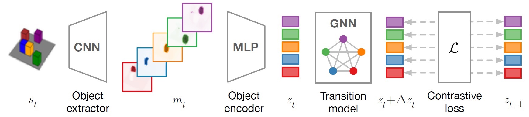
Figure 11. Action model with a hybrid knowledge representation (Kipf et al.,, 2020). Firstly, the object extractor (a CNN) receives an image representation of the current state $s_{t}$ and outputs a set of object masks $m_{t}$, used to extract the objects in $s_{t}$ (each one associated with a different color in the image). Secondly, the object encoder (an MLP) receives $m_{t}$ and returns a set of abstract object states $z_{t}$. Thirdly, the transition model (a GNN) receives $z_{t}$ and the action to apply to each object as inputs, and predicts the resulting abstract state $z_{t}+\Delta z_{t}$. This prediction is then compared with the ground truth $z_{t+1}$, in order to train the model.

4.1.2. Task-specific action models

Unlike the techniques previously discussed, these methods learn a model specifically tailored for a task or set of tasks, i.e., a task-specific action model. This model represents the dynamics of the environment and, additionally, encodes task-related knowledge which results useful for solving the corresponding tasks. Techniques for learning task-specific action models can be further categorized according to how they integrate this extra knowledge inside the action model.

Value-equivalent action models. The dynamics of complex environments are very difficult to model accurately (as task-general action models try to do), since states are composed of a large number of interrelated elements. However, in most cases only a subset of these state features are actually relevant for the task at hand. Value-equivalent models (Grimm et al.,, 2020) are a type of subsymbolic action models which, instead of being trained to predict the next state as accurately as possible, learn a state representation useful for predicting the value, i.e., reward, of future states. Thanks to this, they learn to only focus on task-relevant state features and abstract away those aspects of the environment not useful to solve the task. One of the most successful implementations of this idea can be found in MuZero (Schrittwieser et al.,, 2020). This work extends the AlphaZero (Silver et al.,, 2018) algorithm to the scenario where no action model is provided a priori. MuZero learns a value-equivalent action model which is used by the MCTS planning procedure to predict the value of future states and select the best action. MuZero achieved state-of-the-art results on the Atari video game environment and matched the performance of AlphaZero on Go, chess and shogi. Value Prediction Networks (Oh et al.,, 2017) follow a similar approach, training an action model which learns to predict future rewards and values (see Figure 12). This model is then used by a b-best, d-depth search algorithm instead of MCTS, where b and d are hyperparameters. In a similar fashion, the Predictron (Silver et al.,, 2017) learns an action model which can be repeatedly rolled forward to predict the value of the state received as input.

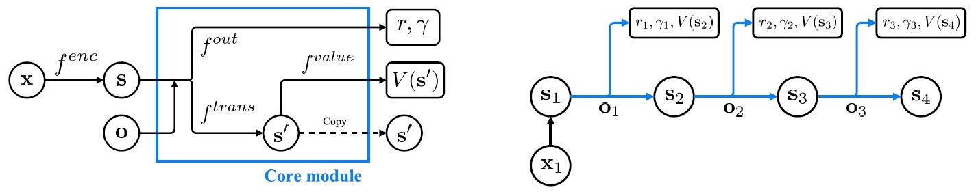
Figure 12. Value Prediction Network (Oh et al.,, 2017). Left: value-equivalent action model. It receives as inputs a state $x$ and an option $o$ (instead of an action). The encoding module $f^{enc}$ maps $x$ to an abstract state $s$, the outcome module $f^{out}$ predicts the reward $r$ and discount factor $\gamma$ associated with executing $o$ at $s$, the transition module $f^{trans}$ predicts the next abstract state $s^{\prime}$ and, lastly, the value module $f^{value}$ estimates the value $V(s^{\prime})$ of $s^{\prime}$. Right: the action model is unrolled multiple times to perform planning.

Hierarchical action models. These models distribute knowledge across multiple levels of hierarchy or abstraction. The bottom level represents the environment dynamics in a general, task-independent way akin to task-general action models. Then, one or more higher levels encode specific, task-dependent knowledge which facilitates the resolution of the corresponding task. The main methods for representing hierarchical knowledge are temporally-extended actions (Sutton et al.,, 1999), goals (Aha,, 2018) and hierarchical decomposition methods (Georgievski and Aiello,, 2015).

Temporally-extended actions (Sutton et al.,, 1999), also known as macroactions (Korf,, 1985) and options (Sutton et al.,, 1999), are a type of abstract, high-level actions whose execution extends across several time steps, as opposed to primitive, low-level actions which are applied in just one step. A set of options defined over an MDP constitutes a semi-Markov Decision Process (SMDP) (Sutton et al.,, 1999), a special type of MDP where actions take variable amounts of time to finish (see Figure 13). Options consist of three components: a policy, an initiation set and a termination condition. In order to start executing an option, the current state must belong to the initiation set. Once started, the agent selects actions according to the option policy until the termination condition is met. Options make possible to group actions which are often executed together. In AP, this translates into a reduction in the depth of the search tree (Jiménez et al.,, 2012) whereas, in RL, options facilitate exploration and value propagation, which in turn speeds up learning (McGovern and Sutton,, 1998). Nevertheless, options also increase the number of alternatives to choose from at each state. For this reason, it is important to carefully consider how many options to use. Options have been successfully learned and applied to both the field of AP (Fikes et al.,, 1972; Botea et al.,, 2005; Coles and Smith,, 2007) and RL (Stolle and Precup,, 2002; Machado et al.,, 2017; Konidaris and Barto,, 2007).

Figure 13. Options, MDPs and SMDPs (Sutton et al.,, 1999). Top: MDP, where an action (black dot in the image) is executed at each time step. Middle: SMDP, where the execution of options (empty dots in the image) takes several time steps. Bottom: options over MDP, where the execution of an option (empty dot) results in the execution of several actions (black dots) until the option terminates.

Goal Reasoning (Aha,, 2018) provides a design philosophy for agents whose behaviour revolves around goals. It makes possible to design agents which do not only learn how to obtain a particular goal but also reason about what should be the goal to achieve in the first place. This is especially important for dynamic environments where unexpected events (discrepancies) may require a change in the goals to pursue. Goal-Driven Autonomy (GDA) (Molineaux et al.,, 2010) provides a general framework for goal-reasoning agents that detect discrepancies, generate possible explanations for them, formulate new goals and manage (prioritize) the pending goals. (Jaidee et al.,, 2012) uses Case-based Reasoning (Kolodner,, 2014) and RL to learn to detect discrepancies, associate them to new goals and learn policies to achieve the selected goals. (Weber et al.,, 2012) proposes an agent which learns to formulate goals using expert demonstrations for the StarCraft game. (Pozanco et al., 2018a, ) learns to predict future goals based on current and past states and performs an anticipatory planning process which considers both current and future goals. (Núñez-Molina et al.,, 2022) proposes a neurosymbolic method which combines DRL with SP to select and achieve goals in order to reduce planning times. Finally, in RL goals have also been utilized as a method to improve exploration (Forestier et al.,, 2017; Laversanne-Finot et al.,, 2018). These methods learn a goal space from which goals are sampled in order to direct exploration towards interesting regions of the state space.

Hierarchical decomposition methods make possible to split a complex problem into a series of subproblems so that the total computational effort of solving these subproblems is smaller than if the original problem had been directly addressed. The most common way to perform this decomposition is provided by Hierarchical Task Networks (HTN) (Georgievski and Aiello,, 2015). HTN domains contain a set of tasks, which can be grouped in either primitive or compound. Primitive tasks correspond to actions that can be directly executed in the environment, in a similar fashion to PDDL actions. Conversely, compound tasks cannot be directly executed and need to be decomposed into a series of primitive or compound tasks. Every compound task has associated one or more decomposition methods, representing different ways to achieve the same task. Each decomposition method has some preconditions which must be true in order to be applied and defines a sequence of subtasks the original task can be decomposed into (see Figure 14). HTN planners receive as inputs an HTN domain and a compound task to achieve, known as the goal task. Then, they find a valid decomposition of the goal task as a sequence of primitive tasks by repeatedly applying the decomposition methods available. There exist a wide variety of HTN planners such as NOAH (Sacerdoti,, 1975), Nonlin (Tate,, 1977), SIPE-2 (Wilkins,, 1990), O-Plan2 (Tate et al.,, 1994) SHOP2 (Nau et al.,, 2003), SIADEX (Castillo et al.,, 2006) and Tree-REX (Schreiber et al.,, 2019). One issue of HTN planning is the substantial time investment needed to encode HTN domains. To alleviate this burden, several methods have been developed to automatically learn HTN domains from data (Hogg et al.,, 2008; Nejati et al.,, 2006; Chen et al.,, 2021). This learning data is comprised of a set of plan traces obtained from experts, often along with some additional information such as annotated tasks or partial method definitions.

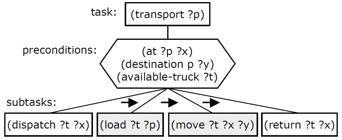
Figure 14. Example of an HTN decomposition method (Nau et al.,, 2003). The depicted method decomposes the compound task transport into four subtasks, two of which are also compound (dispatch and return) and two of which are primitive (load and move).

4.2. Domain exploitation

An action model defines the structure of the MDP. Some aspects of this structure are explicitly encoded in the action model description, e.g., the available actions and environment dynamics. However, other properties of the MDP, such as state invariants and landmarks, do not appear in this description. Throughout the years, many techniques have tried to learn this additional structural information with different purposes, such as facilitating the resolution of the MDP or generating data for training some of the methods discussed in Section 3. Unlike methods for learning action models, this field lacks a proper structure. Thus, we propose to group these techniques under the name domain exploitation. In addition, we further categorize them in methods that learn information about the entire domain and those which only learn information about a specific task.

4.2.1. Task-general domain exploitation

These methods learn general information about the entire domain and do not focus on any particular task of such domain. We discuss four different approaches: state invariants, state space clustering, planning problem generation and scenario planning.

State invariants. These are properties which hold true for every valid, i.e., reachable, state of the MDP. The most widely-known invariant type corresponds to mutex constraints (Blum and Furst,, 1997), which declare that several state properties are mutually exclusive, i.e., cannot be true at the same time. For example, in the blocksworld domain, a block $X_{1}$ can never be on top of more than one other block at the same time, i.e., the set of atoms $\{on(X_{1},X_{2}),...,on(X_{1},X_{n})\}$ are pair-wise mutually exclusive for all $n$ blocks at the state. Another invariant is given by the exactly-n constraint which, given a set $P=\{p_{1},p_{2},...,p_{m}\}$ of properties, states that exactly $n$ properties from $P$ must be true in every MDP state. For example, at each blocksworld state $s$, the arm must either be holding one block $X_{i}$ (i.e., $holding(X_{i})\in s$) or be empty (i.e., $handempty()\in s$). This corresponds to an exactly-1 invariant where $P=\{holding(X_{1}),...,holding(X_{n}),handempty()\}$. There exist many methods for automatically extracting state invariants given a symbolic (e.g., PDDL) domain description. Most methods (Helmert,, 2009; Gerevini and Schubert,, 1998; Rintanen,, 2008) extract invariants via inductive reasoning: they prove that, if a given invariant is true at some state $s$, it will remain true at all successor states $s^{\prime}$ of $s$ (i.e., those obtained by executing an applicable action at $s$). Some methods follow a different aproach. For instance, TIM (Fox and Long,, 1998) represents the behaviour of objects in the domain using finite state machines and forms classes of objects that share the same behaviour. These classes are then used to infer a rich type structure along with different state invariants. Finally, state invariants have many applications in SP. For example, the FD planner (Helmert,, 2006) needs to extract mutex constraints in order to translate the planning task from PDDL to a different encoding in terms of multi-valued variables, whereas the STAN (Long and Fox,, 1999) planner leverages the state invariants extracted by TIM in order to enhance system performance.

State space clustering. Some methods apply clustering techniques to the state space of the MDP. They group states together according to a notion of similarity or distance between states, which must be properly defined in order to obtain clusters with the desired qualities. This definition can incorporate information about the task at hand or be completely task-agnostic. Thus, some state space clustering techniques are task-general and obtain a clustering for the entire domain while others are task-specific and focus on obtaining a clustering suitable for a concrete task. Additionally, several methods require a symbolic description of the MDP whereas others do not impose this restriction. (Singh et al.,, 1995) proposes a RL algorithm that groups together states $s$ with similar value $V(s)$ using a form of soft aggregation, where a state belongs to each cluster with a certain probability. The RL agent learns a value function at the cluster level, and calculates the value of a given state as the weighted sum of the values of the clusters it belongs to. (Feyzabadi and Carpin,, 2017) partitions the MDP state space into a smaller number of abstract states or clusters (see Figure 15) and uses the resulting abstract MDP to compute the optimal policy in a more efficient manner. The clustering algorithm employed groups together states that are connected and have similar reward value. In SP, the most widely used approach for state clustering selects a subset $P$ of state variables (e.g., atoms), called a pattern, and assigns any two MDP states $s_{i},s_{j}$ to the same abstract state (i.e., cluster) if they share the same value for all variables in $P$. The clustering obtained is then often leveraged to calculate a planning heuristic, known as a pattern database heuristic, based on distances computed over the abstract state space induced by the pattern $P$ (Edelkamp,, 2001, 2007; Rovner et al.,, 2019).

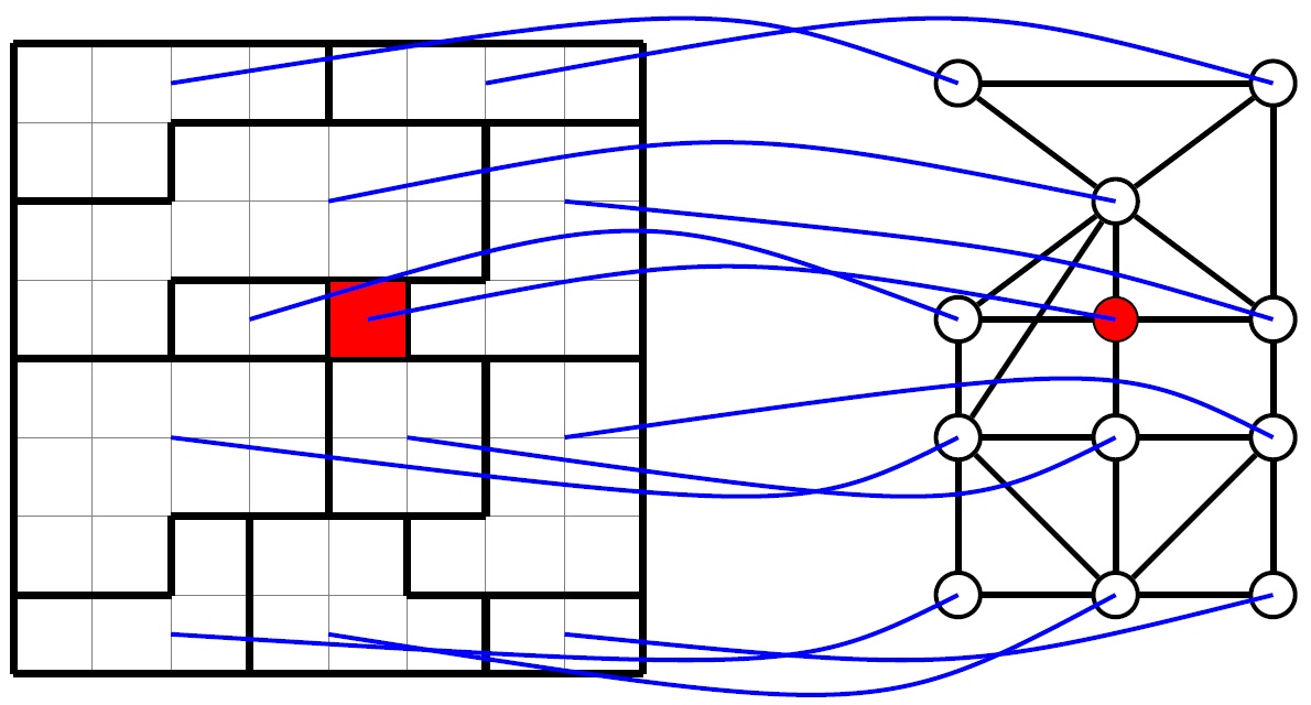
Figure 15. State space clustering (Feyzabadi and Carpin,, 2017). Left: original MDP, where small grid cells represent the states and irregularly shaped cells (indicated by thick lines) represent the state clusters. Right: abstract MDP resulting from the clustering process. Absorbing states in the MDP are colored in red.

Planning problem generation. Given a planning domain, we may be interested in obtaining a set of planning problems pertaining to that particular domain. Among other applications, they can be used as training data for methods that apply ML to SP (e.g., (Shen et al.,, 2020; Balduccini,, 2011)) and as benchmarks to compare the performance of different planning techniques (Vallati et al.,, 2015). In most situations, these problems need to be created by hand or produced by hard-coded, domain-specific problem generators, which requires great effort from the human designers. Nonetheless, there exist several methods in the literature for automatically generating planning problems. For example, (Fern et al.,, 2004) generates problems through random walks. It randomly generates an initial state $s_{0}$ and executes $n$ actions at random to arrive at another state $s_{n}$. Then, it selects a subset of the atoms of $s_{n}$, which constitutes the goal $g$, and returns the corresponding planning problem $(s_{0},g)$. The problems generated with this method are always solvable but they may be inconsistent, i.e., the initial state $s_{0}$ generated may correspond to an impossible situation of the world (e.g., in blocksworld, a state where a block is simultaneously on top of two blocks). (Fuentetaja and De la Rosa,, 2012) also employs a random walk approach but is able to generate problems that are valid, i.e., both solvable and consistent. To achieve this, it receives as inputs the domain description along with some additional information that determines the characteristics of the problems generated, in order to preserve consistency. (Torralba et al.,, 2021) proposes Autoscale, a method that leverages domain-specific generators in order to obtain problems that are valid, diverse and of graded difficulty, for their use in planning competitions. (Núñez-Molina et al.,, 2023) proposes NeSIG, a neurosymbolic method that uses DRL to learn to generate problems for a given PDDL domain, so that they are valid, diverse and difficult to solve (see Figure 16). Lastly, (Katz and Sohrabi,, 2020) generates complete planning tasks (i.e., domain and problem pairs) that are difficult, diverse and of a particular causal structure specified by the user.

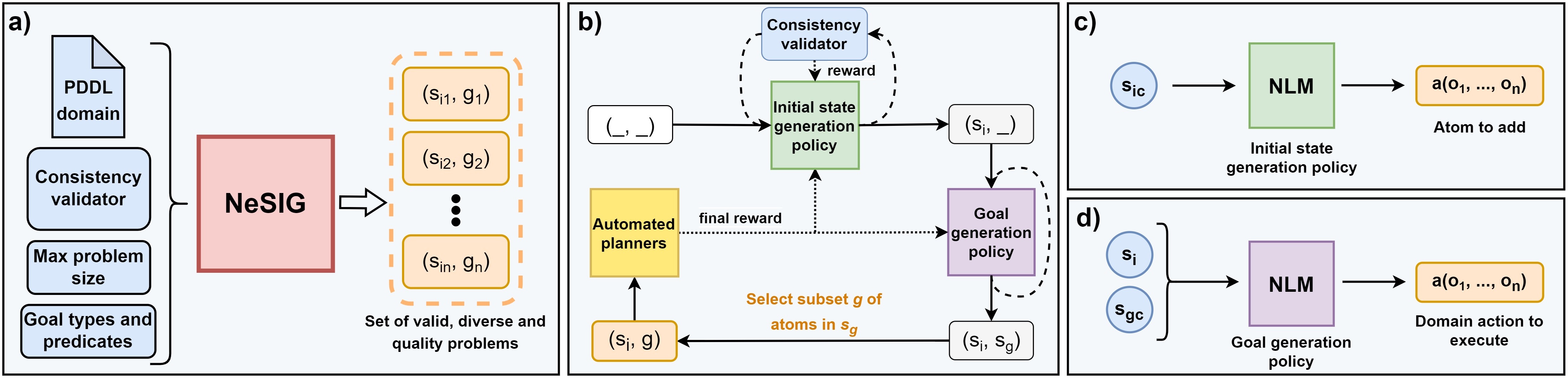
Figure 16. NeSIG (Núñez-Molina et al.,, 2023). a) Architecture overview. NeSIG receives a PDDL domain description, a set of consistency rules (consistency validator in the image) and some additional information; it outputs a set of valid, diverse and difficult problems for the corresponding domain. b) Policy training with RL. NeSIG starts from an empty problem $(\_,\_)$. Then, it iteratively adds objects and atoms to it, which are selected by the initial state generation policy, in order to generate the initial state $s_{i}$. Next, it applies actions to $s_{i}$, which are selected according to the goal generation policy, in order to generate the goal state $s_{g}$. Finally, the goal $g$ is obtained by selecting a subset of the atoms in $s_{g}$, and the generated problem $(s_{i},g)$ is returned. The reward signal for training the policies is obtained from the consistency validator and a planner, which is used to solve the problem and obtain its difficulty (final reward in the image). c) Initial state generation policy. A Neural Logic Machine (NLM) (Dong et al.,, 2019) receives a partially-generated initial state $s_{ic}$ and outputs the next atom to add to it. d) Goal generation policy. An NLM receives a totally-generated initial state $s_{i}$ and a partially-generated goal state $s_{gc}$ and outputs the next action to execute at $s_{gc}$.

Scenario planning. This is a decision support technique where the goal is to generate a variety of possible future scenarios to help organizations foresee the future and adapt to it. (Katz et al.,, 2021) proposes a semi-automatic, neurosymbolic method for performing scenario planning in the real world. It uses DNNs to extract forces and their causal relations from a set of documents encoded in natural language. These forces are the elements of study in scenario planning, e.g., pandemic, lockdown and loss of benefits. The causal relations between forces determine what causes what, e.g., pandemic may cause lockdown which in turn may cause loss of benefits. Once this information has been extracted, it is translated into a PDDL planning domain and problem, which can then be solved with a symbolic planner. The solutions (plans) found by the planner correspond to possible future scenarios, which can be provided to human experts for their analysis.

4.2.2. Task-specific domain exploitation

We now present methods that, instead of extracting information about the entire domain, focus on a specific problem/task and its solution. In this work, we discuss three different approaches: goal recognition/inverse RL, landmark detection and policy validation (including safe RL).

Goal recognition & inverse RL. Goal recognition, also referred to as plan recognition, is the problem of finding the goals that best explain the observed behaviour of an agent. This has many applications such as risk management (Sohrabi et al.,, 2019), video games (Synnaeve and Bessiere,, 2011) and network monitoring (Sohrabi et al.,, 2013). (Ramírez and Geffner,, 2009) follows a plan recognition as planning approach. Instead of using a library of plans, the proposed method only needs to know the planning domain, the possible set $G$ of goals and a partially observed plan $p$ representing the behaviour of the agent. Then, the authors use standard SP techniques to find those goals $g\in G$ for which the optimal plan that achieves them is compatible with the observations in $p$ (see Figure 17). Several works have extended this approach, such as (Sohrabi et al.,, 2016), which provides a relaxation of the problem formulation that allows it to consider noisy and missing observations.

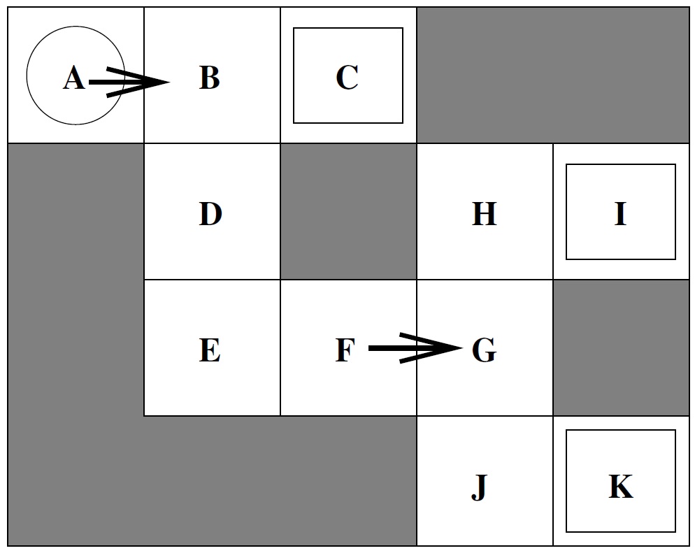
Figure 17. Plan recognition in a navigation domain (Ramírez and Geffner,, 2009). Room A (marked with a circle) is the initial position of the agent, while rooms C, I and K (marked with a square) are its possible destinations. The partially observed plan $p$ contains two observations, $A\rightarrow B$ and $F\rightarrow G$, corresponding to the movements of the agent from room A to B and from room F to G, respectively. Given the observed behaviour, the only possible destinations are I and K but not C. This is because the optimal plan that reaches room C from A is not compatible with the observation $F\rightarrow G$, i.e., the agent does not need to go from F to G in order to reach C.

In the context of RL, goal recognition is known by the name of inverse RL. Here, a different formulation is employed, in terms of rewards instead of goals. The aim of inverse RL is to infer the reward function being optimized by an agent, given its policy or some observations about its behaviour. Some example applications are helicopter control (Abbeel et al.,, 2007), path planning in robotics (Kim and Pineau,, 2016) and fuel-efficient driving (Vogel et al.,, 2012). (Ng et al.,, 2000) provides a foundational method to address this problem. It takes an expert’s policy as input and utilizes linear programming to obtain the reward function that maximally differentiates the input policy from others, in terms of their optimality. (Choi and Kim,, 2011) follows a different approach. It uses Bayesian inference to estimate the posterior probability of the reward functions, given some prior distribution over them and the observed behaviour data. The authors resort to gradient-based optimization in order to efficiently calculate the reward function that maximizes this posterior probability distribution. A comprehensive survey of inverse RL is provided in (Arora and Doshi,, 2021).

Landmark detection. In SP, landmarks are properties (or actions) that must be true (or executed) at some point for every plan that solves a particular planning problem. Landmarks have been successfully applied to a wide range of problems, such as computing planning heuristics (Karpas and Domshlak,, 2009), performing goal recognition (Pereira et al.,, 2020) and planning in multi-agent environments (both cooperative (Maliah et al.,, 2017) and competitive (Pozanco et al., 2018b, )). One of the most widely used methods for automatically obtaining planning landmarks can be found in (Hoffmann et al.,, 2004). Given the description of a CP task, this work is able to extract as landmarks those facts (propositions) which must necessarily be made true during the execution of any solution plan. The proposed method also approximates the order in which these landmarks must be achieved, and encodes this information as a directed graph where the nodes correspond to landmarks and the edges to order restrictions between them. Then, this graph is used to decompose the planning task into smaller sub-tasks. An iterative algorithm is used where, at each step, the leaf nodes of the graph (corresponding to those landmarks that can be directly achieved) are handed to the planner as goals and deleted from the graph. This process is repeated until all the landmarks have been achieved. The experiments carried out by the authors show this method can significantly reduce planning times when used in conjunction with state-of-the-art planners. (Höller and Bercher,, 2021) presents a method to automatically extract landmarks for HTN planning. The proposed method represents the HTN task with an AND/OR graph which is used to obtain different types of landmarks corresponding to facts, actions and methods. The authors show this technique is able to extract more than twice the number of landmarks obtained by other methods, which can then be employed to improve the time performance of HTN planners.

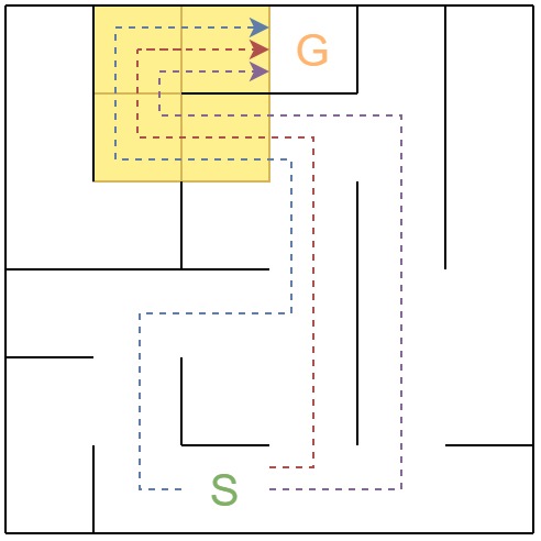
Figure 18. Landmarks in a navigation domain. The agent starts at cell $S$ and must get to cell $G$. The dotted arrows represent different possible paths (plans). No matter the chosen path, the yellow cells will always need to be traversed in order to reach $G$. Thus, they correspond to (state) landmarks in this planning task.

Policy validation & safe RL. Given an MDP and a policy (or plan), we may be interested in testing whether the policy actually corresponds to a valid solution of the MDP or not. This problem receives the name of policy (or plan) validation. In SP, one of the most important plan validation systems is VAL (Howey et al.,, 2004), which was initially developed to automatically validate the plans produced as part of the 3rd International Planning Competition (Long and Fox,, 2003). It can check whether a given plan, represented in PDDL format, is executable and achieves the corresponding goals. In case the plan is flawed, VAL gives advice on how the user can fix it, thus supporting mixed-initiative planning. Additionally, VAL provides different visualization options and supports advanced PDDL features such as actions with continuous effects. Another form of plan validation can be found in the plan monitoring process carried out by online planning architectures. These systems, which interleave planning and execution, must be able to detect discrepancies, i.e., unexpected events that require a modification in the behaviour of the agent. For example, the goal reasoning framework proposed in (Molineaux et al.,, 2010) allows agents to detect discrepancies, infer their causes and generate new goals to pursue, which may require a new plan.

Policy safety is a very important aspect of policy validation. Given a policy, we may be interested in determining if there exists some state in the MDP for which our policy performs very poorly. Safe RL tries to address this issue. It comprises RL techniques which, in addition to maximizing reward, satisfy certain criteria regarding the performance (safety) of the system during the learning and/or deployment processes. This is especially important for real-world environments with critical safety requirements, such as helicopter flight (Koppejan and Whiteson,, 2011) and gas turbine control (Hans et al.,, 2008). One possible approach to safe RL is to transform the reward function so that it includes some notion of risk. For example, (Heger,, 1994) proposes a pessimistic version of the classical Q-Learning algorithm. Instead of predicting the average long-term reward $Q(s,a)$ associated with a state $s$ and action $a$, it estimates the minimum possible return (under the optimal policy) for $(s,a)$. This way, it learns the policy that maximizes the expected return for the worst-case scenario. Other works focus on adapting the exploration process followed by the agent in order to learn the policy. In (Thomaz et al.,, 2006), a human user is allowed to guide an RL agent. The human teacher can provide feedback to the agent in the form of a reward function and, additionally, restrict the set of actions the agent can take at any given moment. Thanks to this guidance, the RL agent is able to learn the optimal policy more efficiently while exploring the state space in a safer way. A comprehensive survey of safe RL can be found in (Garcıa and Fernández,, 2015).

5. Towards an ideal method for SDM

In this section, we try to provide further insight into the existing methods for solving MDPs. Firstly, we propose to categorize these methods along two main dimensions: how they solve the MDP and how they represent their knowledge. Secondly, we discuss what properties an ideal method for SDM should exhibit. Based on these properties, we then analyse the advantages and disadvantages of the different approaches for solving MDPs.

We note that the existing methods for solving MDPs differ from one another in two main aspects. Firstly, they differ in the approach employed to obtain the solution of the MDP. Some methods (e.g., AP algorithms) use an action model to synthesize their solution, often by performing a reasoning process over it. Conversely, other methods (e.g., model-free RL algorithms) do not require a model of the MDP and, instead, learn their solution using the data obtained by interacting with the environment. Secondly, methods for solving MDPs differ in the type of knowledge representation employed. Whereas some methods represent their knowledge symbolically using a formal, logic-based language (e.g., PDDL), other methods encode their knowledge subsymbolically, usually into the weights of a DNN.

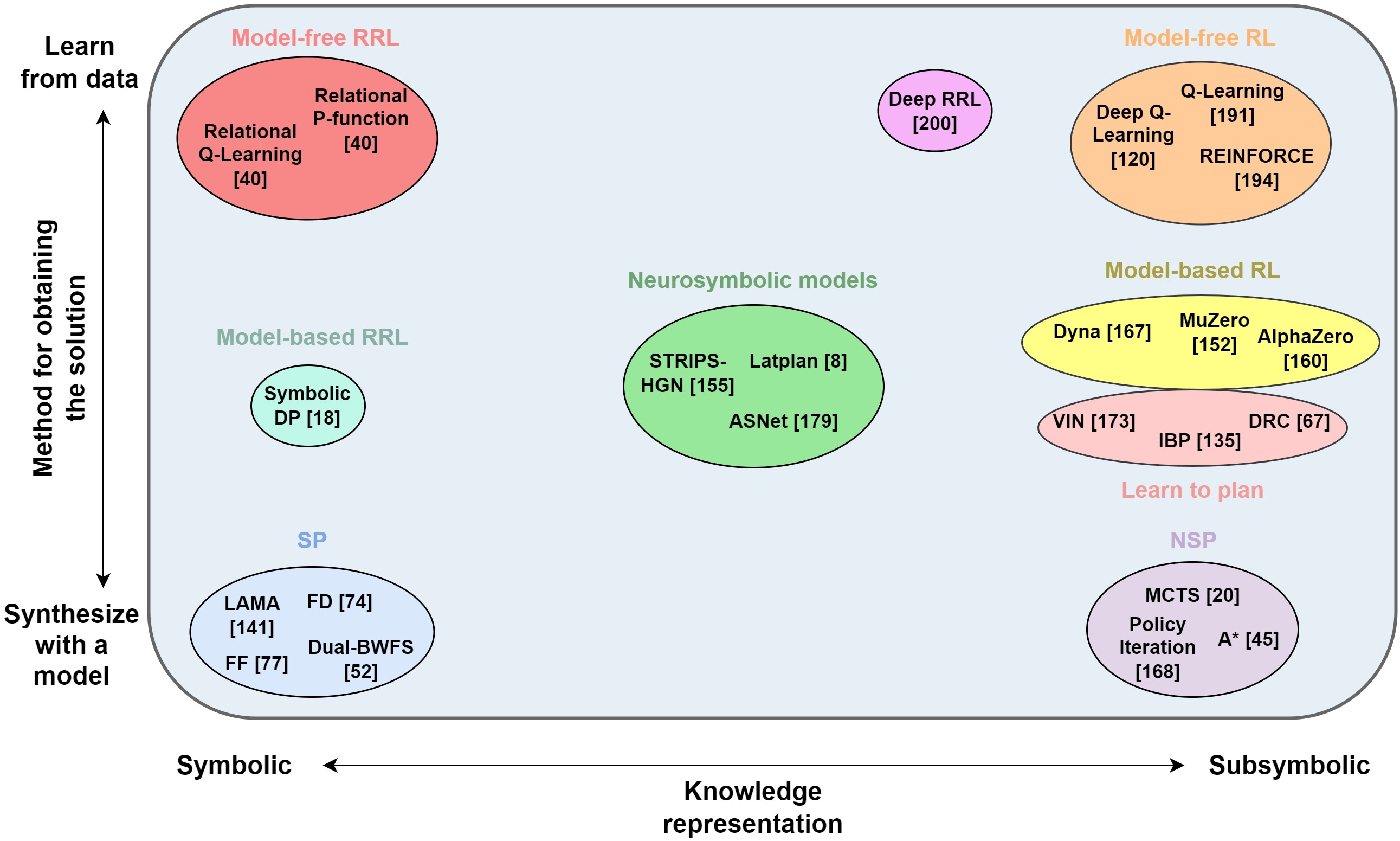
Figure 19. Diagram of methods according to their knowledge representation and method for obtaining the solution. Methods placed in the middle of an axis represent hybrid approaches that combine the two extremes of the corresponding axis, i.e., methods that both learn from data and synthesize the solution with a model (Y axis) and methods that integrate symbolic and subsymbolic knowledge representations (X axis). Colored bubbles are used to group similar methods together.

Figure 19 shows a diagram with different methods for solving MDPs, organized according to how they solve the MDP (Y axis) and how they represent their knowledge (X axis). The bottom of the diagram contains methods that employ an action model to synthesize the solution of the MDP, i.e., AP methods. AP methods that employ a symbolic knowledge representation, i.e., SP methods, are placed on the bottom left corner of the diagram, whereas those with a subsymbolic representation, i.e., NSP methods, are placed on the bottom right corner. The top of the diagram corresponds to methods that do not require an action model and instead learn the MDP solution from the data obtained by interacting with the environment, i.e., model-free RL methods. Most model-free RL methods, from both tabular RL and DRL, represent their knowledge subsymbolically and, thus, are placed on the top right corner of the diagram. Some of them, known as model-free RRL, do employ a symbolic knowledge representation and, hence, are placed on the top left corner. Some RL methods, known as model-based RL, leverage an action model in order to learn the solution of the MDP. Since they combine the two alternative methods for obtaining the MDP solution, they are placed in the middle of the Y axis on the diagram. Model-based RL methods that employ a subsymbolic knowledge representation are placed on the middle right part of the diagram, whereas those with a symbolic representation, known as model-based RRL, are placed on the middle left. The middle right part of the diagram also corresponds to those methods that learn to plan, as they represent their knowledge subsymbolically and both employ an action model and learn their solution from data. The Deep RRL method proposed in (Zambaldi et al.,, 2018) corresponds to a model-free RL algorithm (thus placed on the top of the diagram) that employs a DNN with a relational inductive bias in the form of an attention mechanism. Therefore, this work uses a subsymbolic knowledge representation that shares some properties with symbolic ones and, hence, is placed between the middle and right part of the X axis. Finally, neurosymbolic models combine both methods for obtaining the solution, the learn from data of RL and synthesize with a model of AP, and additionally integrate the symbolic and subsymbolic knowledge representations. This is why they are placed in the middle of our diagram.

In light of so many different approaches for solving MDPs, we may wonder what are the advantages and disadvantages of the existing methods. In order to answer this question, we first discuss what properties an ideal AI for SDM should exhibit. We frame this question from the perspective of a user who simply wants to solve a particular SDM task in the best way possible. Firstly, an ideal SDM method should be applicable to any task posed by the user. Secondly, the method should be easy to use, requiring as little human effort as possible. Thirdly, it should solve the task efficiently. Fourthly, it should be interpretable by the user. Fifthly, the solution obtained by the method should generalize to other tasks different from the one it was obtained for. These requirements give shape to five different properties that result desirable for MDP-solving methods:

• Applicability. An ideal method for SDM should be capable of solving all different sorts of MDPs. Nonetheless, there exist many characteristics that make MDPs more difficult to solve and, thus, limit the applicability of SDM methods. In this work, we have focused on two of them: stochasticity and partial observability (i.e., POMDPs). A few other MDP features that limit applicability are: continuity (i.e., MDPs with continuous state spaces $S$ and/or action spaces $A$), multiple agents (e.g., games like chess where an opponent must be beaten), noisy state observations (e.g., a robot with faulty sensors) and/or noisy actions (e.g., a robot with faulty actuators), the size of the state space, and the complexity of the MDP dynamics.

• Ease of use. This property refers to the amount of human effort needed to adapt an SDM method to a particular task, so the larger the effort, the harder it is to use. An ideal method for SDM should require as little human effort as possible. The amount of effort is directly proportional to the quantity of prior knowledge (about the MDP to solve) required by the method and how difficult it is to encode this knowledge in a suitable representation for it.

• Efficiency. An ideal method for SDM should obtain the solution of the MDP as efficiently as possible. In Computer Science, efficiency is usually measured in terms of the time and space (i.e., memory) an algorithm needs to solve a problem. Analogously, efficiency in AP is usually measured as the time a method spends to find the MDP solution or, alternatively, as the number of tasks from a set that it is able to solve given some time and memory limits, what is known as coverage. On the other hand, efficiency in RL is often measured as the amount of data a method needs to achieve a certain performance, what is known as data-efficiency.

• Interpretability. In recent years, there has been great interest in developing interpretable/explainable AI (XAI) (Gunning and Aha,, 2019) systems for many different applications, including SDM (Chakraborti et al.,, 2020). An ideal SDM method should be fully interpretable, i.e., humans should be able to understand how it works, the characteristics of the solution obtained by the method and the reasons behind the actions it takes. In addition to understanding and verifying the system, interpretability allows to modify its behaviour, thus opening the door to building collaborative systems where humans and SDM methods cooperate to solve problems, as in Mixed-Initiative Planning.

• Generalizability. In some cases, we may be interested in solving not one but a set of different (although similar) MDPs. Solving each MDP separately may be computationally intractable if the number of MDPs in the set is very large (or even infinite). For this reason, an ideal method for SDM should be able to generalize, i.e., the solution obtained by the method for a particular MDP should also be applicable to solve other similar MDPs.

We now leverage these five desirable properties to compare the different existing methods for solving MDPs, assessing their advantages and disadvantages.

Regarding applicability, most subsymbolic methods manage many different types of MDPs either off the self or with some minor modifications. For example, Deep Q-Learning naturally manages non-determinism and has been extended to also manage partial observability and noise (Hausknecht and Stone,, 2015), and continuous state and action spaces (Gu et al.,, 2016). On the other hand, the symbolic community has historically focused on solving the CP case so, even though there exist symbolic methods capable of managing aspects such as non-determinism (Cimatti et al.,, 2003) and partial observability (Draper et al.,, 1994), their support is currently more limited than the one provided by subsymbolic methods. We believe the reason behind this is that, in order to manage these extensions to the CP case, symbolic techniques require more complex methods for representing knowledge (e.g., PPDDL (Younes and Littman,, 2004) instead of PDDL for non-determinism) and reasoning with it, which must be designed by humans, as opposed to subsymbolic techniques where a DNN usually takes care of everything and naturally manages all these aspects. Therefore, subsymbolic methods exhibit better applicability, in general, than symbolic ones. Additionally, it may be the case that we do not have access to an action model (e.g., the MDP dynamics are unknown) and we cannot learn it with the methods described in Section 4.1 because either we lack the necessary data or the dynamics are too complex to learn. In these scenarios, methods that synthesize the MDP solution with a model, such as AP, cannot be employed. Therefore, these methods exhibit worse applicability than those that learn their solution from data without a model, such as model-free RL.

Regarding ease of use, SDM methods that require an action model (e.g., AP) are harder to use than those which do not (e.g., model-free RL). This is due to the fact that, as previously commented, in some situations the action model cannot be learned and needs to be designed by a human expert, thus requiring additional human effort. Additionally, symbolic methods generally require more human effort, and thus provide worse ease of use, than subsymbolic ones. Symbolic methods require knowledge to be represented symbolically, in a logic-based language such as PDDL. Nonetheless, some MDPs may be hard to describe in terms of a set of objects and their relations/interactions, so obtaining a logical representation for them may require extensive human effort. On the other hand, subsymbolic methods often impose no restrictions on how knowledge must be represented, so the user can choose whichever representation scheme (including symbolic ones) that minimizes the effort needed to encode this knowledge. For example, subsymbolic model-based RL methods such as AlphaGo and Dyna are indifferent to how the action model is represented, as long as it allows them to obtain the next state $s^{\prime}$ and reward $r$ associated with a given state-action $(s,a)$ pair.

The efficiency of SDM methods is directly proportional to the amount of task knowledge that they leverage. On the one hand, methods that employ an action model are usually more efficient than those which do not. For example, it has been shown that model-based RL achieves higher data-efficiency than model-free RL (Kaiser et al.,, 2019). On the other hand, symbolic representations often provide more knowledge than their subsymbolic counterparts and, hence, result in higher efficiency. For instance, SP techniques make use of powerful domain-independent heuristics to speed up search which, in order to be computed, require a symbolic description of the action model (Keyder et al.,, 2014) or of states and goals (Frances et al.,, 2017), so they cannot be exploited by AP methods with purely subsymbolic representations.

Regarding interpretability, SDM methods that synthesize their solution with a model (e.g., AP) tend to be more interpretable than those which do not (e.g., model-free RL). This is mainly due to the fact that methods in the first category solve the MDP via an iterative process, carrying out a series of steps which can then be analyzed in order to provide insight that is out of reach for model-free methods. For instance, (Magnaguagno et al.,, 2017) provides a visualization tool of the search tree of SP algorithms, showing the heuristic value for different stages of the search. This results useful for understanding how different planners solve the task, step by step. Additionally, symbolic methods are more interpretable than subsymbolic ones, as they represent their knowledge in a formal, logic-based language that results comprehensible to humans (or, at least, human experts). For example, PDDL action models explicitly state what are the effects of each action, whereas subsymbolic models do not. Another example is the solution obtained by symbolic methods. Regardless of whether it corresponds to a plan (e.g., as in CP) or policy (e.g., as in Generalized Planning), this solution is encoded in a logic-based language and, hence, results more interpretable than the one obtained by subsymbolic methods (e.g., a policy encoded in the weights of a DNN).

Finally, generalizability depends on the specific scope of each SDM method. Some methods (e.g., CP algorithms) focus on solving a single MDP, whereas others (e.g., Generalized Planning and most DRL algorithms) aim to solve a set of different MDPs. Given the same scope, policies that carry out an iterative process over an action model in order to select the action to execute, i.e., deliberative policies, often generalize better than those which do not, i.e., reactive policies. For instance, (Tamar et al.,, 2016) shows that deliberative policies learned by VINs generalize better than reactive policies when applied to new problems of the same domain. Besides, representing knowledge symbolically also helps achieve good generalization. Two examples are RRL, where FOL-based representations are leveraged in order to generalize to tasks with different number of objects, and DNNs with relational inductive biases (Zambaldi et al.,, 2018), which generalize better than purely subsymbolic DNNs.

To summarize, SDM methods that synthesize the MDP solution with a model exhibit better efficiency, interpretability and generalizability, whereas methods that learn their solution from data, without a model, are more widely applicable and easier to use. Analogously, symbolic methods present better efficiency, interpretability and generalizability, whereas subsymbolic methods present better applicability and ease of use. As a result of this analysis, we conclude that the two competing paradigms for obtaining the MDP solution (synthesizing it with a model versus learning it from data) and representing knowledge (symbolically versus subsymbolically) are complementary, as the shortcomings of each one correspond to the strengths of the other. Therefore, we argue that an ideal method for SDM should integrate these different approaches into the same architecture: it should both learn and plan in order to obtain its solution, and combine the symbolic and subsymbolic representations for its knowledge. As shown in Figure 19, neurosymbolic methods perform this integration, which is why they are situated in the center of the diagram. Therefore, we believe neurosymbolic AI poses a very promising approach towards achieving an ideal method for SDM, one that would exhibit the five desirable properties detailed in this section.

6. Future Directions

This review has helped us to identify promising future directions to further advance the field of SDM via the integration of symbolic and subsymbolic AI. We now mention some of these proposals:

• Interpretability. The interpretability of AI systems has become a big concern in recent years due to the ever-increasing ubiquity of such systems, especially in safety-critical applications. Despite advancements in the fields of DL and DRL to design more interpretable architectures such as GNNs, the symbolic approach still has the upper hand when it comes to interpretability. Neurosymbolic methods allow to integrate the capabilities of DL and DRL to extract complex patterns from data with the interpretability of classical symbolic representations such as PDDL. They pose a promising approach towards building systems that do not only solve tasks in an effective and efficient manner, but which are also able to explain their decisions (actions) to a human supervisor. Additionally, it would be interesting to explore representations not only interpretable by human experts like PDDL, but by any human user like natural language.

• Human-machine collaboration. The current paradigm for problem solving entails building autonomous systems based on DL and DRL which try to rely on the user as little as possible. However, in most real-world scenarios, humans have access to crucial domain-specific knowledge which can greatly facilitate the learning process of the agent. The main difficulty in providing this information to the system comes from the fact that the knowledge representation commonly employed in modern AI, based on DNNs, is very different to that used by humans. Thus, in order to achieve effective human-machine collaboration, it is essential to reconcile these two representations. One possibility is provided once again by neurosymbolic methods, since these techniques utilize symbolic representations that are understandable by humans (experts). An alternative approach is to implement a communication interface capable of translating between the subsymbolic representation of the AI system and one understandable by humans (e.g., natural language). Regardless of the chosen method, the integration of both types of representation will make possible to build AI systems that effectively communicate and cooperate with humans. For example, users will be able to easily provide prior knowledge to the agent and guide its behaviour during the task-solving process. Additionally, it would also be useful that the agent itself could query the human for assistance when needed, e.g., in order to escape a dead-end situation.

• Goal Reasoning. Goal Reasoning allows to create AI systems which are capable of reasoning about their own goals. This is similar to the way we humans think, as our actions are influenced by a set of goals, intentions, desires, etc. which are not fixed but rather vary with time. Thus, Goal Reasoning provides an ideal framework to design AI agents which collaborate with humans. Ideally, such a system should be able to function autonomously, being capable of formulating, selecting and pursuing the necessary goals to achieve the corresponding task. At the same time, the human user should be able to understand the behaviour and intentions of the system and, at any given moment, modify the goals the agent is pursuing. To build such a system, the neurosymbolic approach is a good fit. A neurosymbolic goal reasoning method could use DNNs to build a latent representation of the domain which allowed it to infer interesting goals, encoded in a symbolic representation. Then, a symbolic reasoning method, e.g., an automated planner, could reason about which goals should be pursued at each moment and the specific method for achieving them.

• Symbolic value-equivalent action models. Value-equivalent action models only encode those aspects of the environment dynamics which result useful for the task at hand. This is an essential requirement to learn action models of complex environments, such as those often encountered in real-world tasks, as it is infeasible to accurately depict every aspect of their dynamics. However, so far all value-equivalent action models employ a subsymbolic knowledge representation. We believe this value-equivalence principle would prove even more useful in the case of symbolic action models. Subsymbolic action models employ DNNs to encode their knowledge and, since neural networks are universal approximators, they can accurately represent any aspect of the environment regardless of how complex it is (although learning such a complex representation would require huge amounts of data and would have the risk of overfitting, thus the need for value-equivalent models). On the other hand, some complex environments may be hard (or even impossible) to accurately represent using a symbolic action model, in terms of a set of distinct objects and their relations/interactions. Therefore, when confronted with such kind of environments, we should instead try to obtain a symbolic description of only those aspects of the dynamics that are needed to solve the task at hand, i.e., a symbolic value-equivalent model.

• Neurosymbolic action models. The main idea behind symbolic value-equivalent action models is to find a symbolic description of the environment that results good enough for the task at hand, even if it completely ignores some aspects about the dynamics. However, we might wonder if such a description exists in the first place. For some environments, a symbolic description of their dynamics may prove highly inaccurate and leave out aspects that result crucial to solve the task. For example, it would be infeasible to obtain a high-quality description of the dynamics of a complex physics simulator in PDDL and, thus, the resulting symbolic action model would not be of great use to solve any task in this domain. In these cases, those crucial aspects for which a good symbolic description cannot be obtained should be encoded subsymbolically. This neurosymbolic action model would employ a symbolic representation for those elements of the environment which can be properly encoded in such a way, and a subsymbolic representation for the rest. This approach could, in theory, combine the best of both worlds: the abstraction and interpretability of the symbolic representation with the accuracy and wide applicability of the subsymbolic representation.

7. Conclusions

In this work, we have provided an overview of the main symbolic, subsymbolic and hybrid methods for SDM, focusing on the case of finite MDPs. We have presented both techniques for obtaining the solution of MDPs and for learning information about their structure. We have classified methods for solving MDPs in those that obtain their solution via a reasoning process over a model of the world, known as AP, and those that learn their solution from data, known as RL. Additionally, we have described a new type of methods, capable of learning to plan, which have emerged in recent years. We have classified methods for learning the structure of MDPs in those that learn an action model, i.e., a model of the MDP dynamics required by many MDP-solving methods such as AP and model-based RL, and those that learn additional structural aspects which are not encoded in the action model but may result useful to solve the MDP. We have coined the name domain exploitation to refer to this second group of methods. Afterwards, we have discussed what properties an ideal method for SDM should exhibit. Based on these properties, we have analysed the advantages and disadvantages of the different MDP-solving approaches presented in this work. As a result of our analysis, we have argued that an ideal method for SDM should integrate both paradigms for solving the MDP (the synthesize with a model of AP versus the learn from data of RL) and representing knowledge (symbolically versus subsymbolically). Since neurosymbolic AI actually performs this integration, we have concluded that it poses a promising approach towards achieving an ideal method for SDM. Finally, we have proposed several lines of future work in order to advance the field of SDM via the unification of symbolic and subsymbolic AI.

8. Acknowledgements

This work has been partially funded by the Andalusian Regional Projects B-TIC-668-UGR20 and PYC20-RE-049UGR, the Spanish National Project RTI2018-098460-B-I00 with FEDER funds and the Andalusian Regional predoctoral grant no. 21-111-PREDOC-0039.

We want to thank Dr. Masataro Asai for his valuable feedback when writing this review.

References

- Abbeel et al., (2007) Abbeel, P., Coates, A., Quigley, M., and Ng, A. Y. (2007). An application of reinforcement learning to aerobatic helicopter flight. Advances in neural information processing systems.
- Abbeel and Ng, (2005) Abbeel, P. and Ng, A. Y. (2005). Learning first-order markov models for control. Advances in neural information processing systems.
- Aha, (2018) Aha, D. W. (2018). Goal reasoning: Foundations, emerging applications, and prospects. AI Magazine.
- Aler et al., (2002) Aler, R., Borrajo, D., and Isasi, P. (2002). Using genetic programming to learn and improve control knowledge. Artificial Intelligence.
- Arora et al., (2018) Arora, A., Fiorino, H., Pellier, D., Métivier, M., and Pesty, S. (2018). A review of learning planning action models. The Knowledge Engineering Review.
- Arora and Doshi, (2021) Arora, S. and Doshi, P. (2021). A survey of inverse reinforcement learning: Challenges, methods and progress. Artificial Intelligence.
- Asadi et al., (2018) Asadi, K., Cater, E., Misra, D., and Littman, M. L. (2018). Towards a simple approach to multi-step model-based reinforcement learning. arXiv preprint arXiv:1811.00128.
- Asai et al., (2022) Asai, M., Kajino, H., Fukunaga, A., and Muise, C. (2022). Classical planning in deep latent space. Journal of Artificial Intelligence Research.
- Auer et al., (2002) Auer, P., Cesa-Bianchi, N., and Fischer, P. (2002). Finite-time analysis of the multiarmed bandit problem. Machine learning.
- Balduccini, (2011) Balduccini, M. (2011). Learning and using domain-specific heuristics in asp solvers. AI Communications.
- Battaglia et al., (2016) Battaglia, P., Pascanu, R., Lai, M., Jimenez Rezende, D., et al. (2016). Interaction networks for learning about objects, relations and physics. Advances in neural information processing systems.
- Battaglia et al., (2018) Battaglia, P. W., Hamrick, J. B., Bapst, V., Sanchez-Gonzalez, A., Zambaldi, V., Malinowski, M., Tacchetti, A., Raposo, D., Santoro, A., Faulkner, R., et al. (2018). Relational inductive biases, deep learning, and graph networks. arXiv preprint arXiv:1806.01261.
- Bertsekas, (2019) Bertsekas, D. (2019). Reinforcement learning and optimal control. Athena Scientific.
- Besold et al., (2017) Besold, T. R., Garcez, A. d., Bader, S., Bowman, H., Domingos, P., Hitzler, P., Kühnberger, K.-U., Lamb, L. C., Lowd, D., Lima, P. M. V., et al. (2017). Neural-symbolic learning and reasoning: A survey and interpretation. arXiv preprint arXiv:1711.03902.
- Blum and Furst, (1997) Blum, A. L. and Furst, M. L. (1997). Fast planning through planning graph analysis. Artificial intelligence.
- Botea et al., (2013) Botea, A., Bouzy, B., Buro, M., Bauckhage, C., and Nau, D. S. (2013). Pathfinding in games. In Artificial and Computational Intelligence in Games. Schloss Dagstuhl - Leibniz-Zentrum für Informatik.
- Botea et al., (2005) Botea, A., Enzenberger, M., Müller, M., and Schaeffer, J. (2005). Macro-ff: Improving ai planning with automatically learned macro-operators. Journal of Artificial Intelligence Research.
- Boutilier et al., (2001) Boutilier, C., Reiter, R., and Price, B. (2001). Symbolic dynamic programming for first-order mdps. In International Joint Conference on Artificial Intelligence.
- Brown et al., (2020) Brown, T. B., Mann, B., Ryder, N., Subbiah, M., Kaplan, J., Dhariwal, P., Neelakantan, A., Shyam, P., Sastry, G., Askell, A., et al. (2020). Language models are few-shot learners. Advances in Neural Information Processing Systems.
- Browne et al., (2012) Browne, C. B., Powley, E., Whitehouse, D., Lucas, S. M., Cowling, P. I., Rohlfshagen, P., Tavener, S., Perez, D., Samothrakis, S., and Colton, S. (2012). A survey of monte carlo tree search methods. IEEE Transactions on Computational Intelligence and AI in games.
- Bundy and Wallen, (1984) Bundy, A. and Wallen, L. (1984). Breadth-first search. In Catalogue of artificial intelligence tools. Springer Berlin Heidelberg.
- Burstein and McDermott, (1996) Burstein, M. H. and McDermott, D. V. (1996). Issues in the development of human-computer mixed-initiative planning. In Advances in Psychology. Elsevier.
- Bylander, (1994) Bylander, T. (1994). The computational complexity of propositional strips planning. Artificial Intelligence.
- Cappart et al., (2021) Cappart, Q., Chételat, D., Khalil, E. B., Lodi, A., Morris, C., and Velickovic, P. (2021). Combinatorial optimization and reasoning with graph neural networks. In Proceedings of the Thirtieth International Joint Conference on Artificial Intelligence.
- Castillo et al., (2006) Castillo, L., Fdez-Olivares, J., García-Pérez, Ó., and Palao, F. (2006). Efficiently handling temporal knowledge in an htn planner. In Proceedings of the Sixteenth International Conference on International Conference on Automated Planning and Scheduling.
- Chakraborti et al., (2020) Chakraborti, T., Sreedharan, S., and Kambhampati, S. (2020). The emerging landscape of explainable automated planning & decision making. In International Joint Conference on Artificial Intelligence.
- Chang et al., (2017) Chang, M., Ullman, T., Torralba, A., and Tenenbaum, J. B. (2017). A compositional object-based approach to learning physical dynamics. In International Conference on Learning Representations.
- Charpentier et al., (2021) Charpentier, A., Elie, R., and Remlinger, C. (2021). Reinforcement learning in economics and finance. Computational Economics.
- Chen et al., (2021) Chen, K., Srikanth, N. S., Kent, D., Ravichandar, H., and Chernova, S. (2021). Learning hierarchical task networks with preferences from unannotated demonstrations. In Conference on Robot Learning.
- Chiappa et al., (2017) Chiappa, S., Racanière, S., Wierstra, D., and Mohamed, S. (2017). Recurrent environment simulators. In International Conference on Learning Representations.
- Choi and Kim, (2011) Choi, J. and Kim, K.-E. (2011). Map inference for bayesian inverse reinforcement learning. In Advances in Neural Information Processing Systems.
- Chrisman, (1992) Chrisman, L. (1992). Reinforcement learning with perceptual aliasing: The perceptual distinctions approach. In Proceedings of the 10th National Conference on Artificial Intelligence.
- Cimatti et al., (2003) Cimatti, A., Pistore, M., Roveri, M., and Traverso, P. (2003). Weak, strong, and strong cyclic planning via symbolic model checking. Artificial Intelligence.
- Coles and Smith, (2007) Coles, A. I. and Smith, A. J. (2007). Marvin: A heuristic search planner with online macro-action learning. Journal of Artificial Intelligence Research.
- Deisenroth and Rasmussen, (2011) Deisenroth, M. and Rasmussen, C. E. (2011). Pilco: A model-based and data-efficient approach to policy search. In Proceedings of the 28th International Conference on machine learning.
- Depeweg et al., (2017) Depeweg, S., Hernández-Lobato, J., Doshi-Velez, F., and Udluft, S. (2017). Learning and policy search in stochastic dynamical systems with bayesian neural networks. In International Conference on Learning Representations.
- Diuk et al., (2008) Diuk, C., Cohen, A., and Littman, M. L. (2008). An object-oriented representation for efficient reinforcement learning. In Proceedings of the 25th international conference on Machine learning.
- Dong et al., (2019) Dong, H., Mao, J., Lin, T., Wang, C., Li, L., and Zhou, D. (2019). Neural logic machines. arXiv preprint arXiv:1904.11694.
- Draper et al., (1994) Draper, D., Hanks, S., and Weld, D. S. (1994). Probabilistic planning with information gathering and contingent execution. In Proceedings of the Second International Conference on Artificial Intelligence Planning Systems.
- Džeroski et al., (2001) Džeroski, S., De Raedt, L., and Driessens, K. (2001). Relational reinforcement learning. Machine learning.
- Edelkamp, (2001) Edelkamp, S. (2001). Planning with pattern databases. In Proc. ECP, volume 1, pages 13–24. Citeseer.
- Edelkamp, (2007) Edelkamp, S. (2007). Automated creation of pattern database search heuristics. Lecture Notes in Computer Science.
- Edelkamp et al., (2015) Edelkamp, S., Kissmann, P., and Torralba, A. (2015). Bdds strike back (in ai planning). In Proceedings of the AAAI Conference on Artificial Intelligence.
- Farquhar et al., (2018) Farquhar, G., Rockt aschel, T., Igl, M., and Whiteson, S. (2018). Treeqn and atreec: Differentiable tree planning for deep reinforcement learning. In International Conference on Learning Representations.
- Ferguson et al., (2005) Ferguson, D., Likhachev, M., and Stentz, A. (2005). A guide to heuristic-based path planning. In Proceedings of the international workshop on planning under uncertainty for autonomous systems, international conference on automated planning and scheduling.
- Fern et al., (2004) Fern, A., Yoon, S. W., and Givan, R. (2004). Learning domain-specific control knowledge from random walks. In Proceedings of the Fourteenth International Conference on Automated Planning and Scheduling.
- Feyzabadi and Carpin, (2017) Feyzabadi, S. and Carpin, S. (2017). Planning using hierarchical constrained markov decision processes. Autonomous Robots.
- Fikes et al., (1972) Fikes, R. E., Hart, P. E., and Nilsson, N. J. (1972). Learning and executing generalized robot plans. Artificial intelligence.
- Forestier et al., (2017) Forestier, S., Portelas, R., Mollard, Y., and Oudeyer, P.-Y. (2017). Intrinsically motivated goal exploration processes with automatic curriculum learning. arXiv preprint arXiv:1708.02190.
- Fox and Long, (1998) Fox, M. and Long, D. (1998). The automatic inference of state invariants in tim. Journal of Artificial Intelligence Research.
- Fox and Long, (2003) Fox, M. and Long, D. (2003). Pddl2. 1: An extension to pddl for expressing temporal planning domains. Journal of artificial intelligence research.
- Frances et al., (2018) Frances, G., Geffner, H., Lipovetzky, N., and Ramirez, M. (2018). Best-first width search in the ipc 2018: Complete, simulated, and polynomial variants. IPC2018–Classical Tracks.
- Frances et al., (2017) Frances, G., Ramírez Jávega, M., Lipovetzky, N., and Geffner, H. (2017). Purely declarative action descriptions are overrated: Classical planning with simulators. In International Joint Conference on Artificial Intelligence.
- Fuentetaja and De la Rosa, (2012) Fuentetaja, R. and De la Rosa, T. (2012). A planning-based approach for generating planning problems. In Workshops at the Twenty-Sixth AAAI Conference on Artificial Intelligence.
- Garcıa and Fernández, (2015) Garcıa, J. and Fernández, F. (2015). A comprehensive survey on safe reinforcement learning. Journal of Machine Learning Research.
- Garnelo et al., (2016) Garnelo, M., Arulkumaran, K., and Shanahan, M. (2016). Towards deep symbolic reinforcement learning. arXiv preprint arXiv:1609.05518.
- Garnelo and Shanahan, (2019) Garnelo, M. and Shanahan, M. (2019). Reconciling deep learning with symbolic artificial intelligence: representing objects and relations. Current Opinion in Behavioral Sciences.
- Gehring et al., (2022) Gehring, C., Asai, M., Chitnis, R., Silver, T., Kaelbling, L., Sohrabi, S., and Katz, M. (2022). Reinforcement learning for classical planning: Viewing heuristics as dense reward generators. In Proceedings of the International Conference on Automated Planning and Scheduling.
- Gemici et al., (2017) Gemici, M., Hung, C.-C., Santoro, A., Wayne, G., Mohamed, S., Rezende, D. J., Amos, D., and Lillicrap, T. (2017). Generative temporal models with memory. arXiv preprint arXiv:1702.04649.
- Georgievski and Aiello, (2015) Georgievski, I. and Aiello, M. (2015). Htn planning: Overview, comparison, and beyond. Artificial Intelligence.
- Gerevini and Schubert, (1998) Gerevini, A. and Schubert, L. (1998). Inferring state constraints for domain-independent planning. In AAAI.
- Ghallab et al., (2016) Ghallab, M., Nau, D., and Traverso, P. (2016). Automated planning and acting. Cambridge University Press.
- Gil, (1992) Gil, Y. (1992). Acquiring domain knowledge for planning by experimentation. Technical report, CARNEGIE-MELLON UNIV PITTSBURGH PA DEPT OF COMPUTER SCIENCE.
- Goldman and Boddy, (1996) Goldman, R. P. and Boddy, M. S. (1996). Expressive planning and explicit knowledge. In Proceedings of the Third International Conference on Artificial Intelligence Planning Systems.
- Grimm et al., (2020) Grimm, C., Barreto, A., Singh, S., and Silver, D. (2020). The value equivalence principle for model-based reinforcement learning. In Advances in Neural Information Processing Systems.
- Gu et al., (2016) Gu, S., Lillicrap, T., Sutskever, I., and Levine, S. (2016). Continuous deep q-learning with model-based acceleration. In International conference on machine learning. PMLR.
- Guez et al., (2019) Guez, A., Mirza, M., Gregor, K., Kabra, R., Racanière, S., Weber, T., Raposo, D., Santoro, A., Orseau, L., Eccles, T., et al. (2019). An investigation of model-free planning. In International Conference on Machine Learning.
- Guez et al., (2018) Guez, A., Weber, T., Antonoglou, I., Simonyan, K., Vinyals, O., Wierstra, D., Munos, R., and Silver, D. (2018). Learning to search with mctsnets. In International conference on machine learning.
- Gunning and Aha, (2019) Gunning, D. and Aha, D. (2019). Darpa’s explainable artificial intelligence (xai) program. AI magazine.
- Hans et al., (2008) Hans, A., Schneegaß, D., Schäfer, A. M., and Udluft, S. (2008). Safe exploration for reinforcement learning. In European Symposium on Artificial Neural Networks.
- Haslum et al., (2019) Haslum, P., Lipovetzky, N., Magazzeni, D., and Muise, C. (2019). An introduction to the planning domain definition language. Synthesis Lectures on Artificial Intelligence and Machine Learning.
- Hausknecht and Stone, (2015) Hausknecht, M. and Stone, P. (2015). Deep recurrent q-learning for partially observable mdps. In 2015 aaai fall symposium series.
- Heger, (1994) Heger, M. (1994). Consideration of risk in reinforcement learning. In Machine Learning Proceedings. Elsevier.
- Helmert, (2006) Helmert, M. (2006). The fast downward planning system. Journal of Artificial Intelligence Research.
- Helmert, (2009) Helmert, M. (2009). Concise finite-domain representations for pddl planning tasks. Artificial Intelligence, 173(5-6):503–535.
- Hester and Stone, (2013) Hester, T. and Stone, P. (2013). Texplore: real-time sample-efficient reinforcement learning for robots. Machine learning.
- Hoffmann, (2001) Hoffmann, J. (2001). Ff: The fast-forward planning system. AI magazine.
- Hoffmann et al., (2004) Hoffmann, J., Porteous, J., and Sebastia, L. (2004). Ordered landmarks in planning. Journal of Artificial Intelligence Research.
- Hogg et al., (2008) Hogg, C., Munoz-Avila, H., and Kuter, U. (2008). Htn-maker: Learning htns with minimal additional knowledge engineering required. In Proceedings of the Twenty-Third AAAI Conference on Artificial Intelligence.
- Höller and Bercher, (2021) Höller, D. and Bercher, P. (2021). Landmark generation in htn planning. In Proceedings of the AAAI Conference on Artificial Intelligence.
- Howey et al., (2004) Howey, R., Long, D., and Fox, M. (2004). Val: Automatic plan validation, continuous effects and mixed initiative planning using pddl. In IEEE International Conference on Tools with Artificial Intelligence.
- Jaidee et al., (2012) Jaidee, U., Munoz-Avila, H., and Aha, D. W. (2012). Learning and reusing goal-specific policies for goal-driven autonomy. In International Conference on Case-Based Reasoning.
- Jiménez et al., (2012) Jiménez, S., De La Rosa, T., Fernández, S., Fernández, F., and Borrajo, D. (2012). A review of machine learning for automated planning. The Knowledge Engineering Review.
- Jiménez et al., (2008) Jiménez, S., Fernández, F., and Borrajo, D. (2008). The PELA architecture: integrating planning and learning to improve execution. In National Conference on Artificial Intelligence. AAAI Press.
- Jiménez et al., (2019) Jiménez, S., Segovia-Aguas, J., and Jonsson, A. (2019). A review of generalized planning. The Knowledge Engineering Review.
- Jong and Stone, (2007) Jong, N. K. and Stone, P. (2007). Model-based function approximation in reinforcement learning. In Proceedings of the 6th international joint conference on Autonomous agents and multiagent systems.
- Kaiser et al., (2019) Kaiser, Ł., Babaeizadeh, M., Miłos, P., Osiński, B., Campbell, R. H., Czechowski, K., Erhan, D., Finn, C., Kozakowski, P., Levine, S., et al. (2019). Model based reinforcement learning for atari. In International Conference on Learning Representations.
- Kansky et al., (2017) Kansky, K., Silver, T., Mély, D. A., Eldawy, M., Lázaro-Gredilla, M., Lou, X., Dorfman, N., Sidor, S., Phoenix, S., and George, D. (2017). Schema networks: Zero-shot transfer with a generative causal model of intuitive physics. In International Conference on Machine Learning.
- Karpas and Domshlak, (2009) Karpas, E. and Domshlak, C. (2009). Cost-optimal planning with landmarks. In International Joint Conference on Artificial Intelligence.
- Katz and Sohrabi, (2020) Katz, M. and Sohrabi, S. (2020). Generating data in planning: Sas planning tasks of a given causal structure. HSDIP 2020.
- Katz et al., (2021) Katz, M., Srinivas, K., Sohrabi, S., Feblowitz, M., Udrea, O., and Hassanzadeh, O. (2021). Scenario planning in the wild: A neuro-symbolic approach. FinPlan.
- Keyder et al., (2014) Keyder, E., Hoffmann, J., and Haslum, P. (2014). Improving delete relaxation heuristics through explicitly represented conjunctions. Journal of Artificial Intelligence Research.
- Khansari-Zadeh and Billard, (2011) Khansari-Zadeh, S. M. and Billard, A. (2011). Learning stable nonlinear dynamical systems with gaussian mixture models. IEEE Transactions on Robotics.
- Kim and Pineau, (2016) Kim, B. and Pineau, J. (2016). Socially adaptive path planning in human environments using inverse reinforcement learning. International Journal of Social Robotics.
- Kingma and Welling, (2014) Kingma, D. P. and Welling, M. (2014). Auto-encoding variational bayes. In International Conference on Learning Representations.
- Kipf et al., (2020) Kipf, T., van der Pol, E., and Welling, M. (2020). Contrastive learning of structured world models. In International Conference on Learning Representations.
- Kober et al., (2013) Kober, J., Bagnell, J. A., and Peters, J. (2013). Reinforcement learning in robotics: A survey. The International Journal of Robotics Research.
- Koller et al., (2007) Koller, D., Friedman, N., Džeroski, S., Sutton, C., McCallum, A., Pfeffer, A., Abbeel, P., Wong, M.-F., Meek, C., Neville, J., et al. (2007). Introduction to statistical relational learning. MIT press.
- Kolobov, (2012) Kolobov, A. (2012). Planning with markov decision processes: An ai perspective. Synthesis Lectures on Artificial Intelligence and Machine Learning.
- Kolodner, (2014) Kolodner, J. (2014). Case-based reasoning. Morgan Kaufmann.
- Konidaris and Barto, (2007) Konidaris, G. D. and Barto, A. G. (2007). Building portable options: Skill transfer in reinforcement learning. In International Joint Conference on Artificial Intelligence.
- Koppejan and Whiteson, (2011) Koppejan, R. and Whiteson, S. (2011). Neuroevolutionary reinforcement learning for generalized control of simulated helicopters. Evolutionary intelligence.
- Korf, (1985) Korf, R. E. (1985). Macro-operators: A weak method for learning. Artificial intelligence.
- Kramer, (1996) Kramer, S. (1996). Structural regression trees. In Proceedings of the Thirteenth National Conference on Artificial Intelligence and Eighth Innovative Applications of Artificial Intelligence Conference.
- Krizhevsky et al., (2012) Krizhevsky, A., Sutskever, I., and Hinton, G. E. (2012). Imagenet classification with deep convolutional neural networks. Advances in neural information processing systems.
- Laversanne-Finot et al., (2018) Laversanne-Finot, A., Pere, A., and Oudeyer, P.-Y. (2018). Curiosity driven exploration of learned disentangled goal spaces. In Conference on Robot Learning.
- Leckie and Zukerman, (1998) Leckie, C. and Zukerman, I. (1998). Inductive learning of search control rules for planning. Artificial Intelligence.
- LeCun et al., (2015) LeCun, Y., Bengio, Y., and Hinton, G. (2015). Deep learning. nature.
- Li, (2018) Li, Y. (2018). Deep reinforcement learning. arXiv preprint arXiv:1810.06339.
- Littman, (1996) Littman, M. L. (1996). Algorithms for sequential decision-making. Brown University.
- Long and Fox, (1999) Long, D. and Fox, M. (1999). Efficient implementation of the plan graph in stan. Journal of Artificial Intelligence Research.
- Long and Fox, (2003) Long, D. and Fox, M. (2003). The 3rd international planning competition: Results and analysis. Journal of Artificial Intelligence Research.
- Lovejoy, (1991) Lovejoy, W. S. (1991). A survey of algorithmic methods for partially observed markov decision processes. Annals of Operations Research.
- Machado et al., (2017) Machado, M. C., Bellemare, M. G., and Bowling, M. (2017). A laplacian framework for option discovery in reinforcement learning. In International Conference on Machine Learning.
- Magnaguagno et al., (2017) Magnaguagno, M. C., FRAGA PEREIRA, R., Móre, M. D., and Meneguzzi, F. R. (2017). Web planner: A tool to develop classical planning domains and visualize heuristic state-space search. In 2017 Workshop on User Interfaces and Scheduling and Planning.
- Maliah et al., (2017) Maliah, S., Shani, G., and Stern, R. (2017). Collaborative privacy preserving multi-agent planning. Autonomous agents and multi-agent systems.
- Marcus, (2018) Marcus, G. (2018). Deep learning: A critical appraisal. arXiv preprint arXiv:1801.00631.
- McGovern and Sutton, (1998) McGovern, A. and Sutton, R. S. (1998). Macro-actions in reinforcement learning: An empirical analysis. Computer Science Department Faculty Publication Series.
- Mnih et al., (2016) Mnih, V., Badia, A. P., Mirza, M., Graves, A., Lillicrap, T., Harley, T., Silver, D., and Kavukcuoglu, K. (2016). Asynchronous methods for deep reinforcement learning. In International conference on machine learning.
- Mnih et al., (2013) Mnih, V., Kavukcuoglu, K., Silver, D., Graves, A., Antonoglou, I., Wierstra, D., and Riedmiller, M. (2013). Playing atari with deep reinforcement learning. arXiv preprint arXiv:1312.5602.
- Mnih et al., (2015) Mnih, V., Kavukcuoglu, K., Silver, D., Rusu, A. A., Veness, J., Bellemare, M. G., Graves, A., Riedmiller, M., Fidjeland, A. K., Ostrovski, G., et al. (2015). Human-level control through deep reinforcement learning. nature.
- Moerland et al., (2020) Moerland, T. M., Broekens, J., and Jonker, C. M. (2020). A framework for reinforcement learning and planning. arXiv preprint arXiv:2006.15009.
- Moerland et al., (2023) Moerland, T. M., Broekens, J., Plaat, A., Jonker, C. M., et al. (2023). Model-based reinforcement learning: A survey. Foundations and Trends® in Machine Learning.
- Molineaux and Aha, (2014) Molineaux, M. and Aha, D. (2014). Learning unknown event models. In Proceedings of the AAAI Conference on Artificial Intelligence.
- Molineaux et al., (2010) Molineaux, M., Klenk, M., and Aha, D. (2010). Goal-driven autonomy in a navy strategy simulation. In AAAI Conference on Artificial Intelligence.
- Mourao et al., (2008) Mourao, K., Petrick, R. P., and Steedman, M. (2008). Using kernel perceptrons to learn action effects for planning. In International Conference on Cognitive Systems.
- Nau et al., (2003) Nau, D. S., Au, T.-C., Ilghami, O., Kuter, U., Murdock, J. W., Wu, D., and Yaman, F. (2003). Shop2: An htn planning system. Journal of artificial intelligence research.
- Nejati et al., (2006) Nejati, N., Langley, P., and Konik, T. (2006). Learning hierarchical task networks by observation. In Proceedings of the 23rd international conference on Machine learning.
- Ng et al., (2000) Ng, A. Y., Russell, S. J., et al. (2000). Algorithms for inverse reinforcement learning. In Proceedings of the Seventeenth International Conference on Machine Learning.
- Núñez-Molina et al., (2022) Núñez-Molina, C., Fernández-Olivares, J., and Pérez, R. (2022). Learning to select goals in automated planning with deep-q learning. Expert Systems with Applications, 202:117265.
- Núñez-Molina et al., (2023) Núñez-Molina, C., Mesejo, P., and Fernández-Olivares, J. (2023). Nesig: A neuro-symbolic method for learning to generate planning problems. arXiv preprint arXiv:2301.10280.
- Oates and Cohen, (1996) Oates, T. and Cohen, P. R. (1996). Searching for planning operators with context-dependent and probabilistic effects. Proceedings of the Thirteenth National Conference on Artificial Intelligence and Eighth Innovative Applications of Artificial Intelligence Conference.
- Oh et al., (2017) Oh, J., Singh, S., and Lee, H. (2017). Value prediction network. In Advances in Neural Information Processing Systems.
- Partalas et al., (2008) Partalas, I., Vrakas, D., and Vlahavas, I. (2008). Reinforcement learning and automated planning: A survey. In Artificial Intelligence for Advanced Problem Solving Techniques. IGI Global.
- Pascanu et al., (2017) Pascanu, R., Li, Y., Vinyals, O., Heess, N., Buesing, L., Racanière, S., Reichert, D., Weber, T., Wierstra, D., and Battaglia, P. (2017). Learning model-based planning from scratch. arXiv preprint arXiv:1707.06170.
- Pasula et al., (2007) Pasula, H. M., Zettlemoyer, L. S., and Kaelbling, L. P. (2007). Learning symbolic models of stochastic domains. Journal of Artificial Intelligence Research.
- Pereira et al., (2020) Pereira, R. F., Oren, N., and Meneguzzi, F. (2020). Landmark-based approaches for goal recognition as planning. Artificial Intelligence.
- (138) Pozanco, A., Fernández, S., and Borrajo, D. (2018a). Learning-driven goal generation. AI Communications.
- (139) Pozanco, A., Yolanda, E., Fernández, S., Borrajo, D., et al. (2018b). Counterplanning using goal recognition and landmarks. In International Joint Conference on Artificial Intelligence.
- Ramírez and Geffner, (2009) Ramírez, M. and Geffner, H. (2009). Plan recognition as planning. In International Joint Conference on Artificial Intelligence.
- Richter and Westphal, (2010) Richter, S. and Westphal, M. (2010). The lama planner: Guiding cost-based anytime planning with landmarks. Journal of Artificial Intelligence Research.
- Rintanen, (2008) Rintanen, J. (2008). Regression for classical and nondeterministic planning. In ECAI 2008. IOS Press.
- Rodrigues et al., (2011) Rodrigues, C., Gérard, P., Rouveirol, C., and Soldano, H. (2011). Active learning of relational action models. In International Conference on Inductive Logic Programming.
- Rovner et al., (2019) Rovner, A., Sievers, S., and Helmert, M. (2019). Counterexample-guided abstraction refinement for pattern selection in optimal classical planning. In Proceedings of the International Conference on Automated Planning and Scheduling.
- Russell and Norvig, (2020) Russell, S. J. and Norvig, P. (2020). Artificial Intelligence: A Modern Approach (4th Edition). Pearson.
- Sacerdoti, (1975) Sacerdoti, E. D. (1975). The nonlinear nature of plans. Technical report, STANFORD RESEARCH INST MENLO PARK CA.
- Safaei and Ghassem-Sani, (2007) Safaei, J. and Ghassem-Sani, G. (2007). Incremental learning of planning operators in stochastic domains. In International Conference on Current Trends in Theory and Practice of Computer Science.
- Sanner et al., (2010) Sanner, S. et al. (2010). Relational dynamic influence diagram language (rddl): Language description. Unpublished ms. Australian National University.
- Schäpers et al., (2018) Schäpers, B., Niemueller, T., Lakemeyer, G., Gebser, M., and Schaub, T. (2018). Asp-based time-bounded planning for logistics robots. In International Conference on Automated Planning and Scheduling.
- Schaul et al., (2015) Schaul, T., Horgan, D., Gregor, K., and Silver, D. (2015). Universal value function approximators. In International conference on machine learning.
- Schreiber et al., (2019) Schreiber, D., Pellier, D., Fiorino, H., et al. (2019). Tree-rex: Sat-based tree exploration for efficient and high-quality htn planning. In Proceedings of the International Conference on Automated Planning and Scheduling.
- Schrittwieser et al., (2020) Schrittwieser, J., Antonoglou, I., Hubert, T., Simonyan, K., Sifre, L., Schmitt, S., Guez, A., Lockhart, E., Hassabis, D., Graepel, T., et al. (2020). Mastering atari, go, chess and shogi by planning with a learned model. Nature.
- Segura-Muros et al., (2021) Segura-Muros, J. Á., Pérez, R., and Fernández-Olivares, J. (2021). Discovering relational and numerical expressions from plan traces for learning action models. Applied Intelligence.
- Serina, (2010) Serina, I. (2010). Kernel functions for case-based planning. Artificial Intelligence.
- Shen et al., (2020) Shen, W., Trevizan, F., and Thiébaux, S. (2020). Learning domain-independent planning heuristics with hypergraph networks. In Proceedings of the International Conference on Automated Planning and Scheduling.
- Shen and Simon, (1989) Shen, W. M. and Simon, H. A. (1989). Rule creation and rule learning through environmental exploration. In International Joint Conference on Artificial Intelligence. Morgan Kaufmann.
- Shi et al., (2015) Shi, X., Chen, Z., Wang, H., Yeung, D.-Y., Wong, W.-K., and Woo, W.-c. (2015). Convolutional lstm network: A machine learning approach for precipitation nowcasting. Advances in neural information processing systems.
- Silver, (2005) Silver, D. (2005). Cooperative pathfinding. Proceedings of the First Artificial Intelligence and Interactive Digital Entertainment Conference.
- Silver et al., (2017) Silver, D., Hasselt, H., Hessel, M., Schaul, T., Guez, A., Harley, T., Dulac-Arnold, G., Reichert, D., Rabinowitz, N., Barreto, A., et al. (2017). The predictron: End-to-end learning and planning. In International Conference on Machine Learning.
- Silver et al., (2018) Silver, D., Hubert, T., Schrittwieser, J., Antonoglou, I., Lai, M., Guez, A., Lanctot, M., Sifre, L., Kumaran, D., Graepel, T., et al. (2018). A general reinforcement learning algorithm that masters chess, shogi, and go through self-play. Science.
- Singh et al., (1995) Singh, S. P., Jaakkola, T., and Jordan, M. I. (1995). Reinforcement learning with soft state aggregation. Advances in neural information processing systems.
- Sohrabi et al., (2019) Sohrabi, S., Katz, M., Hassanzadeh, O., Udrea, O., Feblowitz, M. D., and Riabov, A. (2019). Ibm scenario planning advisor: Plan recognition as ai planning in practice. Ai Communications.
- Sohrabi et al., (2016) Sohrabi, S., Riabov, A. V., and Udrea, O. (2016). Plan recognition as planning revisited. In International Joint Conference on Artificial Intelligence.
- Sohrabi et al., (2013) Sohrabi, S., Udrea, O., and Riabov, A. (2013). Hypothesis exploration for malware detection using planning. In Proceedings of the Twenty-Seventh AAAI Conference on Artificial Intelligence.
- Srinivas et al., (2018) Srinivas, A., Jabri, A., Abbeel, P., Levine, S., and Finn, C. (2018). Universal planning networks: Learning generalizable representations for visuomotor control. In International Conference on Machine Learning.
- Stolle and Precup, (2002) Stolle, M. and Precup, D. (2002). Learning options in reinforcement learning. In International Symposium on abstraction, reformulation, and approximation.
- Sutton, (1991) Sutton, R. S. (1991). Dyna, an integrated architecture for learning, planning, and reacting. ACM Sigart Bulletin.
- Sutton and Barto, (2018) Sutton, R. S. and Barto, A. G. (2018). Reinforcement learning: An introduction. MIT press.
- Sutton et al., (1999) Sutton, R. S., Precup, D., and Singh, S. (1999). Between mdps and semi-mdps: A framework for temporal abstraction in reinforcement learning. Artificial intelligence.
- Sutton et al., (2008) Sutton, R. S., Szepesvári, C., Geramifard, A., and Bowling, M. H. (2008). Dyna-style planning with linear function approximation and prioritized sweeping. In Proceedings of the 24th Conference in Uncertainty in Artificial Intelligence.
- Synnaeve and Bessiere, (2011) Synnaeve, G. and Bessiere, P. (2011). A bayesian model for plan recognition in rts games applied to starcraft. In Artificial Intelligence and Interactive Digital Entertainment Conference.
- Tadepalli et al., (2004) Tadepalli, P., Givan, R., and Driessens, K. (2004). Relational reinforcement learning: An overview. In Proceedings of the ICML-2004 workshop on relational reinforcement learning.
- Tamar et al., (2016) Tamar, A., Levine, S., Abbeel, P., Wu, Y., and Thomas, G. (2016). Value iteration networks. In Advances in Neural Information Processing Systems.
- Tarjan, (1972) Tarjan, R. (1972). Depth-first search and linear graph algorithms. SIAM journal on computing.
- Tate, (1977) Tate, A. (1977). Generating project networks. In Proceedings of the 5th international joint conference on Artificial intelligence-Volume 2.
- Tate et al., (1994) Tate, A., Drabble, B., and Kirby, R. (1994). O-plan2: an open architecture for command, planning and control. In Intelligent scheduling.
- Thomaz et al., (2006) Thomaz, A. L., Breazeal, C., et al. (2006). Reinforcement learning with human teachers: Evidence of feedback and guidance with implications for learning performance. In Aaai.
- Torralba et al., (2021) Torralba, A., Seipp, J., and Sievers, S. (2021). Automatic instance generation for classical planning. In Proceedings of the International Conference on Automated Planning and Scheduling.
- Toyer et al., (2018) Toyer, S., Trevizan, F., Thiébaux, S., and Xie, L. (2018). Action schema networks: Generalised policies with deep learning. In Thirty-Second AAAI Conference on Artificial Intelligence.
- Trunda and Barták, (2013) Trunda, O. and Barták, R. (2013). Using monte carlo tree search to solve planning problems in transportation domains. In Mexican International Conference on Artificial Intelligence.
- ús Virseda et al., (2013) ús Virseda, J., Borrajo, D., and Alcázar, V. (2013). Learning heuristic functions for cost-based planning. Planning and Learning.
- Vallati et al., (2015) Vallati, M., Chrpa, L., Grześ, M., McCluskey, T. L., Roberts, M., Sanner, S., et al. (2015). The 2014 international planning competition: Progress and trends. Ai Magazine.
- Vaswani et al., (2017) Vaswani, A., Shazeer, N., Parmar, N., Uszkoreit, J., Jones, L., Gomez, A. N., Kaiser, Ł., and Polosukhin, I. (2017). Attention is all you need. In Advances in neural information processing systems.
- Veloso and Carbonell, (1993) Veloso, M. M. and Carbonell, J. G. (1993). Derivational analogy in prodigy: Automating case acquisition, storage, and utilization. Machine Learning.
- Vogel et al., (2012) Vogel, A., Ramachandran, D., Gupta, R., and Raux, A. (2012). Improving hybrid vehicle fuel efficiency using inverse reinforcement learning. In Proceedings of the AAAI Conference on Artificial Intelligence.
- Wahlström et al., (2015) Wahlström, N., Schön, T. B., and Deisenroth, M. P. (2015). From pixels to torques: Policy learning with deep dynamical models. arXiv preprint arXiv:1502.02251.
- Walsh and Littman, (2008) Walsh, T. J. and Littman, M. L. (2008). Efficient learning of action schemas and web-service descriptions. In Proceedings of the Twenty-Third AAAI Conference on Artificial Intelligence.
- Wang et al., (2005) Wang, J. M., Fleet, D. J., and Hertzmann, A. (2005). Gaussian process dynamical models. In Advances in Neural Information Processing Systems.
- Wang et al., (2018) Wang, W. Y., Li, J., and He, X. (2018). Deep reinforcement learning for nlp. In Proceedings of the 56th Annual Meeting of the Association for Computational Linguistics: Tutorial Abstracts.
- Wang, (1996) Wang, X. (1996). Learning planning operators by observation and practice. PhD thesis, Carnegie Mellon University.
- Watkins, (1989) Watkins, C. J. C. H. (1989). Learning from delayed rewards. PhD thesis, King’s College.
- Weber et al., (2012) Weber, B., Mateas, M., and Jhala, A. (2012). Learning from demonstration for goal-driven autonomy. In Proceedings of the AAAI Conference on Artificial Intelligence.
- Wilkins, (1990) Wilkins, D. E. (1990). Can ai planners solve practical problems? Computational intelligence.
- Williams, (1992) Williams, R. J. (1992). Simple statistical gradient-following algorithms for connectionist reinforcement learning. Machine learning.
- Yang et al., (2018) Yang, F., Lyu, D., Liu, B., and Gustafson, S. (2018). PEORL: integrating symbolic planning and hierarchical reinforcement learning for robust decision-making. In Proceedings of the Twenty-Seventh International Joint Conference on Artificial Intelligence.
- Yang et al., (2007) Yang, Q., Wu, K., and Jiang, Y. (2007). Learning action models from plan examples using weighted max-sat. Artificial Intelligence.
- Yoon and Kambhampati, (2007) Yoon, S. and Kambhampati, S. (2007). Towards model-lite planning: A proposal for learning & planning with incomplete domain models. In ICAPS2007 Workshop on Artificial Intelligence Planning and Learning.
- Yoon et al., (2006) Yoon, S. W., Fern, A., and Givan, R. (2006). Learning heuristic functions from relaxed plans. In Proceedings of the Sixteenth International Conference on Automated Planning and Scheduling.
- Younes and Littman, (2004) Younes, H. L. and Littman, M. L. (2004). Ppddl1.0: An extension to pddl for expressing planning domains with probabilistic effects. Techn. Rep. CMU-CS-04-162.
- Zambaldi et al., (2018) Zambaldi, V., Raposo, D., Santoro, A., Bapst, V., Li, Y., Babuschkin, I., Tuyls, K., Reichert, D., Lillicrap, T., Lockhart, E., et al. (2018). Deep reinforcement learning with relational inductive biases. In International Conference on Learning Representations.
- Zhuo and Yang, (2014) Zhuo, H. H. and Yang, Q. (2014). Action-model acquisition for planning via transfer learning. Artificial intelligence.