Interpretability for Conditional Coordinated Behavior in Multi-Agent Reinforcement Learning

Abstract

We propose a model-free reinforcement learning architecture, called distributed attentional actor architecture after conditional attention (DA6-X), to provide better interpretability of conditional coordinated behaviors. The underlying principle involves reusing the saliency vector, which represents the conditional states of the environment, such as the global position of agents. Hence, agents with DA6-X flexibility built into their policy exhibit superior performance by considering the additional information in the conditional states during the decision-making process. The effectiveness of the proposed method was experimentally evaluated by comparing it with conventional methods in an objects collection game. By visualizing the attention weights from DA6-X, we confirmed that agents successfully learn situation-dependent coordinated behaviors by correctly identifying various conditional states, leading to improved interpretability of agents along with superior performance.

I Introduction

Explainable reinforcement learning (XRL) has attracted considerable attention in the academic and industrial domains. Several XRL categories exist for the interpretability of agents [21]. For instance, the decision-making process of agents has been interpreted by decomposing reward functions [8] or visualizing their saliency maps based on the integrated gradients method [25]. The attention mechanism developed by [26], in addition to the transformer, also plays a critical role in imparting transparency to the decision-making process. Consequently, various neural network models based on the attention mechanism and transformer, such as vision transformer [4] and decision transformer [1], have enabled the successful visualization of the input information that plays a key role in achieving the state of the art performance in computer vision and even deep reinforcement learning (DRL).

However, few studies have focused on XRL in multi-agent systems (MAS), although clarification of the black-box coordination/cooperation mechanism is crucial in inducing better productivity and robustness for the entire system. Multi-actor-attention-critic (MAAC) [6], incorporating the attention mechanism in the style of MADDPG [13], demonstrated the way agents selectively focus on cooperation among themselves using the attention mechanism. [17, 18] developed an approach to establish the interpretability of agents’ coordinated behaviors by analyzing the individual agent’s attention mechanism and empirically clarified that their agents would selectively identify other agents worthy of coordination. Such findings are expected to improve the explainability of learned behaviors of individuals as well as the efficiency of the entire system. Meanwhile, agents in MAS must behave flexibly depending on the conditions and situations that include other agents and their actions. Agents can learn such conditional behaviors using the aforementioned methods; however, these methods are not sufficient to ensure that the interpretability of the learning results will make agents acquire the expected conditional behaviors.

To address this challenge, we proposed distributed attentional actor architecture after conditional attention (DA6-X). The model architecture is based on reusing the saliency vector [18] to enhance the interpretability of learned conditional coordinated behaviors in multi-agent DRL (MADRL). DA6-X is a sequential framework that combines a module for recognition of the conditions/situations, with any DRL head (corresponding to ’X’), to output the learned behavior. Unlike the previous models [17, 18], DA6-X takes two-layered data: conditional states (conditions/situations) and local observations. DA6-X first represents the conditional states using the saliency vector in the former conditional module (CM). The saliency vector is then reused along with the local observations to feed to the latter local transformer encoder, such that DA6-X is capable of comprehensive learning under various situations. In addition, agents with DA6-X (DA6-X) not only learn condition-dependent actions in a more organized manner but also provide information for understanding the justification and rationale of their actions. By extracting the attention weights from the local transformer encoder in DA6-X, attention heatmaps are generated to determine the parts of the input data describing the conditional aspects that affect the intensity of interests in the two-layered data, especially local observation. This information also helps us understand how conditional states affect the agents’ behaviors, even when the same local observations are provided.

Our primary contributions are summarized as follows:

1. DA6-X, a novel MADRL architecture, was designed for interpreting situation-dependent/conditional coordinated behaviors by reusing the saliency vector.

2. While providing transparency, DA6-X can be easily integrated with any DRL algorithm (hence, X is included in the name) in single-agent or multi-agent DRL systems.

3. DA6-X agents with various conditional states achieve better performance than several existing algorithms taking the objects collection game as an example.

4. Improved interpretable coordinated behaviors are qualitatively demonstrated via the attention mechanism by hierarchically analyzing the input information.

II Related Work

Attention-based method in XRL: In addition to developing research on visual explanations, such as feature-based [7], embedding-based [16], perturbation-based [29], and gradient-based methods [25], incorporation of the attention mechanism in models is one of the most popular methods in XRL [27]. Recently, DA3-X [18] was proposed as an extension of MAT-DQN [17] to demonstrate how decentralized agents build coordination by highlighting the influence of relevant tasks, other agents, and the noise in local observations based on the attention mechanism.

However, these prior studies only represent the influential segments of the agents’ inputs in an aggregated manner by focusing on the performance improvement and ignoring the dependencies within the inputs, i.e., they do not determine the segments in the inputs that direct the agent’s attention to other parts of segments. In contrast, our proposed method explicitly classifies the input information into conditional segments, such as the global positions of the observing agent and other agents, and baseline segments, such as the local visible region, to identify the parts in the conditional segments that affect the agents’ focus of interest within their local observations and result in the development of conditional, situation-dependent, and coordinated behaviors.

Attention Mechanism in MADRL: Various MADRL models utilize the attention mechanism. Several studies [2, 6] use the attention mechanism as a centralized communication processor that efficiently handles encoded messages among agents in MADRL. Incorporation of the attention mechanism in MAS is also beneficial for constrained problems [20], such as approximation of underlying behaviors of agents [11] and trajectory prediction [10]. In particular, [2] introduced the multi-focus attention network, which helps agents attend to important sensory-input information using multiple parallel attentions in a grid-like environment. [28] investigated the enhancement of agents’ ability to efficiently adapt to complicated environments (Box-World and StarCraft II) that require relational reasoning over structured representations using the attention mechanism. [9] introduced joint attention, which aggregates every other agent’s attention map and demonstrates its cost-effectiveness in multi-agent coordination environments.

The early studies on MADRL mainly focused on augmenting the agents’ performance using centralized attention in the centralized training with decentralized execution (CTDE) approach; however, the fully decentralized approach is generally more robust because of less variance in policy updates and is more feasible in realistic domains [14]. Moreover, the qualitative analysis of coordination using attention heatmaps has not been studied in detail. Our goal is to investigate the specific behavioral analysis of cooperative agents based on decentralized attention heatmaps to clarify how to undertake alternative strategies and coordination structures depending on the conditional states and local observations for better interpretability.

III Preliminaries

Dec-POMDP: In this study, the focus is on the decentralized partially observable Markov decision process (dec-POMDP) [22] of $N$ agents, denoted by a tuple $\langle\mathcal{I},\mathcal{S},\{\mathcal{A}_{i}\},p_{T},\{r_{i}\},\{\Omega_{i}\},\mathcal{O},H\rangle$. $\mathcal{I}=\{1,\ldots,N\}$ indicates a set of agents; $\mathcal{S}$ is a finite set of states; and $\mathcal{A}_{i}$ is a finite set of individual action space of $i\in\mathcal{I}$. Suppose $a\in\mathcal{A}$ and $s,s^{\prime}\in\mathcal{S}$; $p_{T}(s^{\prime}|s,a)$ is a transition probability; $r_{i}(s,a)$ is a reward ($\in\mathbb{R}$) obtained by $i\in\mathcal{I}$; $\Omega_{i}$ is a finite set of observations by $i\in\mathcal{I}$; $\mathcal{O}(o|s,a)$ is a transition probability $o\in\Omega$; and $H$ is the time horizon of the process. In dec-POMDP, the agents aim to maximize the discounted cumulative reward $R_{i}=\sum_{t=0}^{H}{\gamma^{t}r_{i}(s,a)}$ by updating their individual policies $\pi_{i}$, where $\gamma$ is a discount factor ($0\leq\gamma<1$).

(a) Object spawn region (green for objects $\bigstar$, red for objects $\blacktriangle$, and beige for both objects $\bigstar$, $\blacktriangle$).

(b) Task execution area, which is partitioned into four distinct regions labeled as $\Gamma$, $\Delta$, $\Theta$, and $\Lambda$.

Figure 1: A grid environment example.

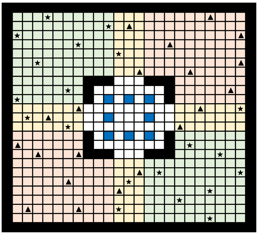
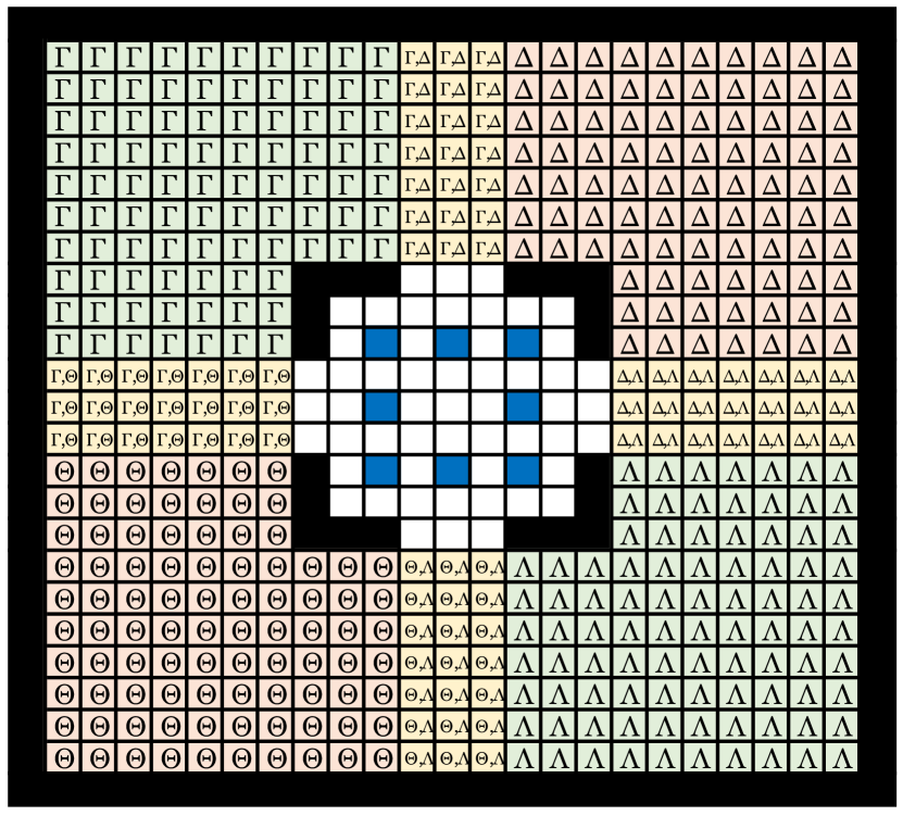
Problem Setting: In the object collection game, agents collect as many objects as possible in a grid-like environment of size $G_{X}\times G_{Y}$, as shown in Fig. 1. At the beginning of each episode, agents are placed at the initial positions indicated by blue cells in Fig. 1 and start exploration. At each step, agents encode the observed local environment in $N_{\mathrm{C}}$ channels of $R_{\mathrm{X}}\times R_{\mathrm{Y}}$ matrices (where $R_{\mathrm{X}}\times R_{\mathrm{Y}}$ is the size of the observation matrices $\in\mathbb{R}^{R_{\mathrm{X}}\times R_{\mathrm{Y}}}$) and feed their local observation in shape of $N_{\mathrm{C}}\times R_{\mathrm{X}}\times R_{\mathrm{Y}}$ into their own networks. Then, they decide the suitable action $a_{i}\in\mathcal{A}_{i}=\{\mathit{up},\mathit{down},\mathit{right},\mathit{left}\}$, wherein each element describes the movement direction of agents for the next step.

Agent $\forall i$ receives a reward $r_{i}$ depending on the condition at the next step, i.e., $i$ obtains a positive reward $r_{\mathrm{o}}>0$ if it moves to the same position as an object; it receives a negative reward $r_{\mathrm{c}}<0$ if it collides against other agents or walls; otherwise, it receives $r_{i}=0$.

Multi-Head Attention: The self-attention mechanism was introduced by [26] to get similarities in sequences as

$$\mathrm{Attention}(Q,K,V)=\mathrm{Softmax}(\frac{Q\cdot K^{T}}{\sqrt{d}})V,$$

where $Q$, $K$, and $V$ denote query, key, and value matrices, respectively, and $d$ is the dimension of the query/key. Multi-head attention (MHA) is determined by calculating the self-attention in $h$ parallel attention heads, as shown in equation below:

$$\begin{split}\mathrm{MHA}(Q,K,V)&=\mathrm{Concat}(\mathit{head}_{1},\ldots,\mathit{head}_{h})W^{O}\\ \mathit{head}_{l}&=\mathrm{Attention}(Q\cdot W_{l}^{Q},K\cdot W_{l}^{K},V\cdot W_{l}^{V}),\end{split}$$

where $W_{l}^{Q}$, $W_{l}^{K}$, $W_{l}^{V}$, $W^{O}$ are projected parameter matrices for attention head $\mathit{head}_{l}$ ($1\leq l\leq h$). The reader is referred to the original paper [26] for more details.

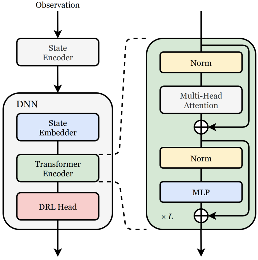
DA3-X: DA3-X [18] is a neural network model comprising the attention mechanism, as shown in Fig. 2. The significance of DA3-X is the interpretability of agents in distributed multi-agent systems. As agents are required to build coordination with other agents in multi-agent systems, it is crucial to clarify how their cooperative behaviors are induced through their black-box decision-making process. A few prior studies worked on the transparency of coordination in centralized multi-agent systems, but mostly they did not assume the distributed system that is more feasible in real-world applications. By using DA3-X as a baseline method, we verified its interpretability as well as its ability to selectively distinguish important segments of observation by analyzing the attention weights in DA3-X. Its versatile network structure where arbitrary reinforcement learning methods can be applied (DA3-DQN, DA3-DDPG, etc.) is also remarkable. Moreover, we verified that it is scale-free with respect to the number of agents as the DA3-X supposes a distributed system and does not depend on models from other agents.

IV Proposed Method: DA6-X

IV-A Neural Network Architecture

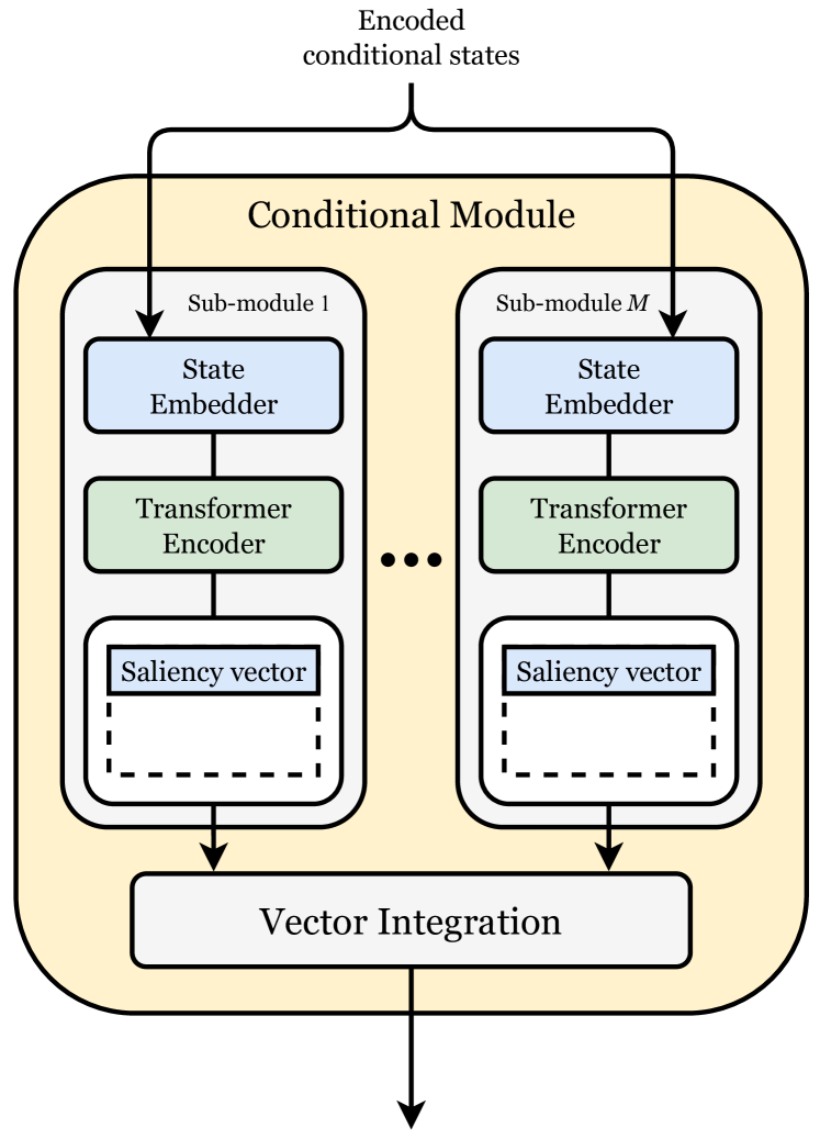
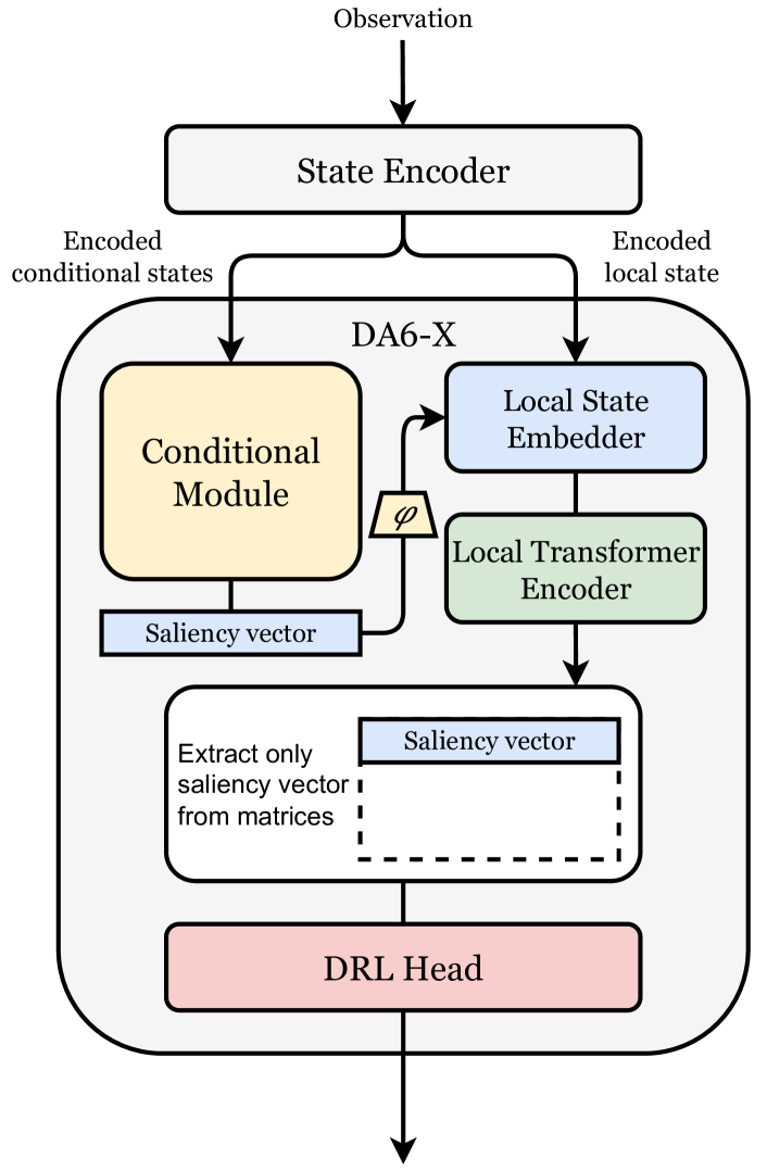
The key idea of DA6-X is to consistently use the same saliency vector in CM and the local transformer encoder, as illustrated in Fig. 2. CM and the local transformer encoder play the roles of recognizing the environmental conditions and weighing the local information by the attention mechanism, respectively. DA6-X is an extension of DA3-X; however, it is different in that DA6-X incorporates CM to explain the rationale for situation-dependent behaviors and to facilitate the understanding of administrators. We incorporated separate transformer encoders in CM to effectively generate the saliency vector. Through the attention mechanism in the transformer encoders in CM, DA6-X can flexibly recognize the conditional states and represent them in the saliency vector that is eventually reused in the local transformer encoders. We can clarify what CM does because it is also interpretable by analyzing the attention weights in the transformer encoders in CM. Similar to the attention analysis demonstrated in Section V-C, further attention analysis of how DA6-X handles the conditional states in CM can be similarly performed. The mathematical procedure of DA6-X is described as follows:

$$\begin{split}g_{m,0}&=[\bm{u}^{\mathrm{sal}}_{m};x^{1}_{m}E^{\mathrm{cond}}_{m};x^{2}_{m}E^{\mathrm{cond}}_{m};\ldots;x^{I_{m}}_{m}E^{\mathrm{cond}}_{m}]+P^{\mathrm{cond}}_{m}\\ g_{m,l}&=\mathrm{TEL}^{\mathrm{cond}}_{m}(g_{m,l-1}),\qquad l=1,\ldots,L_{m}\\ \bm{v}^{\mathrm{sal}}&=\mathrm{VectorIntegration}(g^{0}_{1,L_{1}},\ldots,g^{0}_{m,L_{m}},\ldots,g^{0}_{M,L_{M}})\end{split}$$

The equation above expresses the flow calculations of the conditional states in CM. Suppose there are $M$ submodules in total; the $m$-th $(1\leq m\leq M)$ patched conditional state matrix $x_{m}\in\mathbb{R}^{I_{m}\times(P^{2}_{m}N_{m})}$ is embedded by parameters $E^{\mathrm{cond}}_{m}\in\mathbb{R}^{(P^{2}_{m}N_{m})\times C_{m}}$ and subsequently concatenated with the saliency vector (trainable parameters) $\bm{u}^{\mathrm{sal}}_{m}\in\mathbb{R}^{C_{m}}$, where $I_{m}$ is the length of the $m$-th conditional state after the patched operation; $P_{m}$ is the $m$-th patch size; $N_{m}$ is the number of conditional state channels before the patched operation; and $C_{m}$ is the length of the $m$-th saliency vector. Note that this calculation corresponds to the procedure in the state embedder, as shown in Fig. 2. After positional embedding $P^{\mathrm{cond}}\in\mathbb{R}^{(I_{m}+1)\times C_{m}}$ is appended, the $m$-th input is fed into the $m$-th transformer encoder layer $(\mathrm{TEL}^{\mathrm{cond}}_{m})$, which is illustrated by the green box in Fig. 2. After looping $L_{m}$ times, saliency vector $g^{0}_{1,L_{1}},\ldots,g^{0}_{m,L_{m}},\ldots,g^{0}_{M,L_{M}}$ from all submodules are aggregated in a vector integration procedure to produce the final saliency vector $\bm{v}^{\mathrm{sal}}\in\mathbb{R}^{C_{\mathrm{L}}}$ of length $C_{\mathrm{L}}$.

The calculation after CM is described as follows:

$$\begin{split}h_{0}&=[\varphi(\bm{v}^{\mathrm{sal}});y^{1}E^{\mathrm{local}};y^{2}E^{\mathrm{local}};\ldots;y^{I_{\mathrm{L}}}E^{\mathrm{local}}]+P^{\mathrm{local}}\\ h_{l}&=\mathrm{TEL}^{\mathrm{local}}(h_{l-1}),\qquad l=1,\ldots,L_{\mathrm{L}}\\ Q&=\mathrm{DRLHead}(h^{0}_{L_{\mathrm{L}}})\end{split}$$

After the projection denoted by $\varphi(\cdot)$, the saliency vector $\bm{v}^{\mathrm{sal}}$ is directly fed into the local state embedder, as shown in Fig. 2. Similar to the previous process, the patched local observation $y\in\mathbb{R}^{I_{\mathrm{L}}\times(P^{2}_{\mathrm{L}}N_{\mathrm{L}})}$ is embedded by parameters $E_{\mathrm{L}}\in\mathbb{R}^{(P^{2}_{\mathrm{L}}N_{\mathrm{L}})\times C_{\mathrm{L}}}$ and concatenated to the projected saliency vector $\varphi(\bm{v}^{\mathrm{sal}})$, where $I_{\mathrm{L}}$ is the length of local observation after the patched operation; $P_{\mathrm{L}}$ is the local patch size; and $N_{\mathrm{L}}$ is the number of patched local observation channels. Reusing the saliency vector $\bm{v}^{\mathrm{sal}}$ of CM, DA6-X agents can build flexible policies after considering the conditional states. Similarly, the input is forwarded to the local transformer encoder layer $(\mathrm{TEL}^{\mathrm{local}})$ $L_{\mathrm{L}}$ times after the positional embedding $P^{\mathrm{local}}\in\mathbb{R}^{(I_{\mathrm{L}}+1)\times C_{\mathrm{L}}}$ is appended. Finally, only the saliency vector $h^{0}_{L_{\mathrm{L}}}$ is fed into DRLHead, as shown in Fig. 2.

(a) DA3-X [18].

(b) Conditional Module.

(c) DA6-X.

Figure 2: Architecture of baseline and proposed method.

IV-B Advantages of DA6-X

Because of the selection ability of the attention mechanism, agents achieve higher efficiency in exploration and even better robust coordination than when the attention mechanism is not incorporated in the system. Hence, DA6-X agents with the attention mechanism incorporated are also expected to outperform the conventional MADRL or DRL algorithms, similar to the previous method [17, 18]. In addition, the output of DRLHead denoted as $Q$ in the equation of DA6-X can be Q-values or a stochastic policy, depending on the DRL algorithm to incorporate, such as DDPG [12], PPO [23], or RAINBOW [5]. This feature also leads to higher versatility of DA6-X in real-world applications.

The reuse of the saliency vector in DA6-X is beneficial not only for performance improvement but also for improved interpretability when compared to DA3-X [18]. As explained earlier, DA6-X agents can flexibly change their strategy of weighing a particular piece of information in their local observation depending on an arbitrary number of available conditional states by reusing the saliency vector. Hence, complex behaviors of DA6-X agents can be interpretable using attention heatmaps in their local observation. By contrast, DA3-X agents directly feed the aggregated conditional states to the black-box DRLHead, such that their interpretability in local observations is relatively limited.

The main difference between our proposed method, DA6-X, and DA3-X is CM. Indeed, DA3-X can be regarded as DA6-X without CM ($M=0$) as shown in Fig. 2. Reusing the saliency vector from CM in the latter local transformer encoder, it is interpretable how agents see their local observation after they concern their conditional states in CM, such as their global positions (G pos). Therefore, because of the lack of its CM, DA3-X always acts in the same manner and its interpretability is consistent, whenever its local observation is the same and the conditional states vary. In contrast, DA6-X can flexibly change its way of obtaining the local observation after understanding the conditional states, such that it may act differently depending on the conditional states even though the same local observation is obtained. Because the saliency vector is reused, DA6-X possesses improved interpretability than that of DA3-X.

V Experiments and Results

V-A Experimental Setup

Our experiment was conducted using the objects’ collection game in an environment $\mathcal{E}$, as shown in Fig. 1, where $(G_{X},G_{Y})=(25,25)$, and each color of the cell indicates the entity: black for walls, blue for initial position of agents, white for empty, and green, red, and beige for object spawn regions. Two types of objects were spawned in $\mathcal{E}$: objects $\bigstar$ in green regions, objects of type $\blacktriangle$ in red regions, and both objects in the beige region. The number of objects was set to $20$ for each type ($40$ objects in total). The environment was divided into four distinct sections ($\Gamma$, $\Delta$, $\Theta$, and $\Lambda$), as shown in Fig. 1. Once an agent collected an object, the same type of object was spawned at random location within the spawn region.

TABLE I: Agent-task specification.

Agents	Num	Symbol	Region
Type A	2	$\bigstar$	$\Gamma$, $\Lambda$
Type B	2	$\blacktriangle$	$\Delta$, $\Theta$
Type C	2	$\bigstar$, $\blacktriangle$	$\Gamma$, $\Delta$
Type D	2	$\bigstar$, $\blacktriangle$	$\Theta$, $\Lambda$

Eight agents ($N=8$) were placed at blue cells and learned their individual policies $\pi_{i}$ to collect as many objects as possible without colliding for $5,000$ episodes, where the episode length was $H=200$ steps. These agents were classified into four types, as shown in Table I, which lists the agent type, number of agents, assigned object type, and region to collect. For example, there are two type A agents which collect $\bigstar$ objects in the diagonal regions ($\Gamma$ and $\Lambda$ in Fig. 1), and two type C agents which collect both $\bigstar$ and $\blacktriangle$ objects only in the top-half region ($\Gamma$ and $\Delta$ in Fig. 1). In other words, cooperative agents can be non-cooperative in another region. The reward scheme was set as $r_{\mathrm{o}}=1$ and $r_{\mathrm{c}}=-1$, where $r_{\mathrm{o}}$ is attributed to an agent only when it collects the assigned type object in the allocated region in Table I.

The purpose of our experiment was to analyze the attention weights in the local transformer encoders to investigate how DA6-X agents build situation-dependent coordination when encountering various conditional states and how these conditional states affect their behavioral decisions. We examined eight DA6-DQN agents and DA6-IQN agents, which had the MLP and implicit quantile network (IQN) [3] installed in their DRLHead, respectively. For baseline methods, eight standard DQN agents, IQN agents, DA3-DQN agents, and DA3-IQN agents were trained. In addition to the local observation that was fed into the local state encoder, two types of additional input were provided to the CM: the global position of the observing agent (G pos) and all objects’ positions (O pos) for the conditional states in the environment. Each agent obtains its local observation ($\{R_{\mathrm{X}},R_{\mathrm{Y}}\}=\{7,7\}$) from local view [15]. The baseline agents observe G pos and O pos by relative view [15], while the DA6-X agents obtain the conditional states by merged view [24]. The experiment was repeated three times for each condition by using approximately $100$ GPU hours of NVIDIA GeForce RTX 3090.

(a) Episode reward by DQN-based algorithms.

(b) Episode reward by IQN-based algorithms.

Figure 3: Learning performance comparison with varying conditional states.

TABLE II: Quantitative performance comparison.

Input to CM	Model	Episode reward	Objects counts	Agents collision	Walls collision
None	DQN	$348.64\pm 35.83$	$360.22\pm 35.02$	$6.35\pm 2.50$	$5.23\pm 2.73$
	DA3-DQN	$394.76\pm 34.92$	$402.43\pm 35.07$	$3.94\pm 1.40$	$3.72\pm 1.29$
	IQN	$389.94\pm 28.43$	$398.85\pm 28.48$	$4.30\pm 1.57$	$4.61\pm 1.71$
	DA3-IQN	$402.16\pm 30.44$	$410.41\pm 30.43$	$4.10\pm 1.33$	$4.15\pm 1.69$
G pos	DQN	$282.21\pm 22.75$	$305.59\pm 21.26$	$14.24\pm 6.71$	$9.14\pm 4.32$
	DA3-DQN	$397.94\pm 25.43$	$410.95\pm 25.82$	$7.62\pm 3.68$	$5.38\pm 3.32$
	DA6-DQN	$\mathbf{449.69\pm 24.96}$	$\mathbf{457.08\pm 25.13}$	$\mathbf{3.84\pm 1.21}$	$\mathbf{3.55\pm 1.37}$
	IQN	$147.77\pm 27.12$	$323.51\pm 19.75$	$13.78\pm 7.45$	$161.97\pm 13.42$
	DA3-IQN	$407.29\pm 25.69$	$419.39\pm 24.18$	$6.55\pm 2.85$	$5.55\pm 5.23$
	DA6-IQN	$\mathbf{452.64\pm 25.91}$	$\mathbf{460.65\pm 25.73}$	$\mathbf{4.09\pm 1.40}$	$\mathbf{3.92\pm 1.68}$
G pos + O pos	DQN	$14.60\pm 21.32$	$73.50\pm 10.90$	$39.36\pm 11.93$	$19.54\pm 6.54$
	DA3-DQN	$432.20\pm 22.96$	$446.11\pm 22.33$	$8.46\pm 3.36$	$5.45\pm 2.72$
	DA6-DQN	$\mathbf{456.05\pm 24.28}$	$\mathbf{463.81\pm 24.37}$	$\mathbf{4.04\pm 1.39}$	$\mathbf{3.72\pm 1.10}$
	IQN	$117.73\pm 29.48$	$342.13\pm 15.20$	$19.01\pm 10.28$	$205.40\pm 19.35$
	DA3-IQN	$441.15\pm 19.98$	$455.87\pm 18.72$	$8.37\pm 3.73$	$6.34\pm 4.40$
	DA6-IQN	$\mathbf{479.61\pm 20.30}$	$\mathbf{488.96\pm 19.76}$	$\mathbf{5.30\pm 1.48}$	$\mathbf{4.05\pm 1.47}$

V-B Performance Comparison

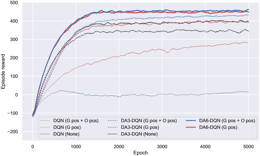
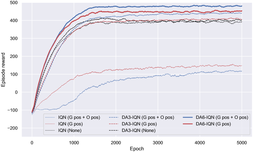
Figure 3 shows the averaged episode reward over $5,000$ episodes for each reinforcement learning method. The color of lines in Fig. 3 are indicatve of the conditional states fed to agents: blue for both G pos and O pos, red for G pos, and black for no conditional states. Table II lists the averaged episode reward, collected number of objects, and collisions that occurred between agents and walls in the final $100$ episode for each learning algorithm and conditional states to CM. In general, learning performance improved when more input information was available during decision-making regardless of the DRL method, and similar phenomena were confirmed except the DQN and IQN agents.

When G pos is available: According to Fig. 3 and Table II, providing the location of observing agents (G pos) resulted in DA3-X and DA6-X agents collecting more objects. DA3-DQN and DA3-IQN agents with G pos collect $8.52$ ($2.12\%$) and $8.98$ ($2.19\%$) more objects when compared with DA3-DQN and DA3-IQN agents, which had no input (None) to CM, while DA6-DQN and DA6-IQN agents with G pos obtain $54.65$ ($13.58\%$) and $50.24$ ($12.24\%$) more objects, thereby achieving $54.93$ and $50.48$ points more in episode rewards. In addition, DA6-DQN and DA6-IQN agents occurred only $7.39$ and $8.01$ collisions in total, which are $43.15\%$ and $33.80\%$ less than those of DA3-DQN and DA3-IQN agents with G pos. Performance degradation is confirmed for the standard DQN and IQN agents with G pos because of its state complexity overload.

When G pos and O pos are available: We confirmed that DA3-X and DA6-X agents achieved even higher learning performance when the location of both observing agents and objects (G pos + O pos) were available. As shown in Table II, DA3-DQN and DA3-IQN agents with G pos and O pos achieve $37.44$ and $38.99$ points more in episode rewards when compared with those of DA3-DQN and DA3-IQN agents without conditional states, while DA6-DQN and DA6-IQN agents improve $61.29$ and $77.45$ points in episode reward. Moreover, the differences in collected objects by DA3-DQN versus DA6-DQN agents and DA3-IQN versus DA6-IQN are $17.69$ ($3.97\%$) and $33.09$ ($7.26\%$), confirming that DA6-X agents successfully build their efficient policy with the conditional states. Similar to the previous case, learning performance by the standard DQN and IQN agents gets worse with G pos and O pos.

V-C Attention and Coordination

It was confirmed that providing conditional states makes DA6-X agents learn more efficient policies. The manner in which the conditional states affect the decision-making process was further investigated to improve the overall performance as well as for successful coordination by analyzing the intensity of the attention weights in particular situations. The coordination analysis was conducted for two cases: when only G pos was available and when G pos and O pos were available.

(a) Solo in $\Delta$.

(b) With type C agent in $\Delta$.

(c) Solo in $\Theta$.

(d) With type C agent in $\Theta$.

Figure 4: Coordination study with G pos.

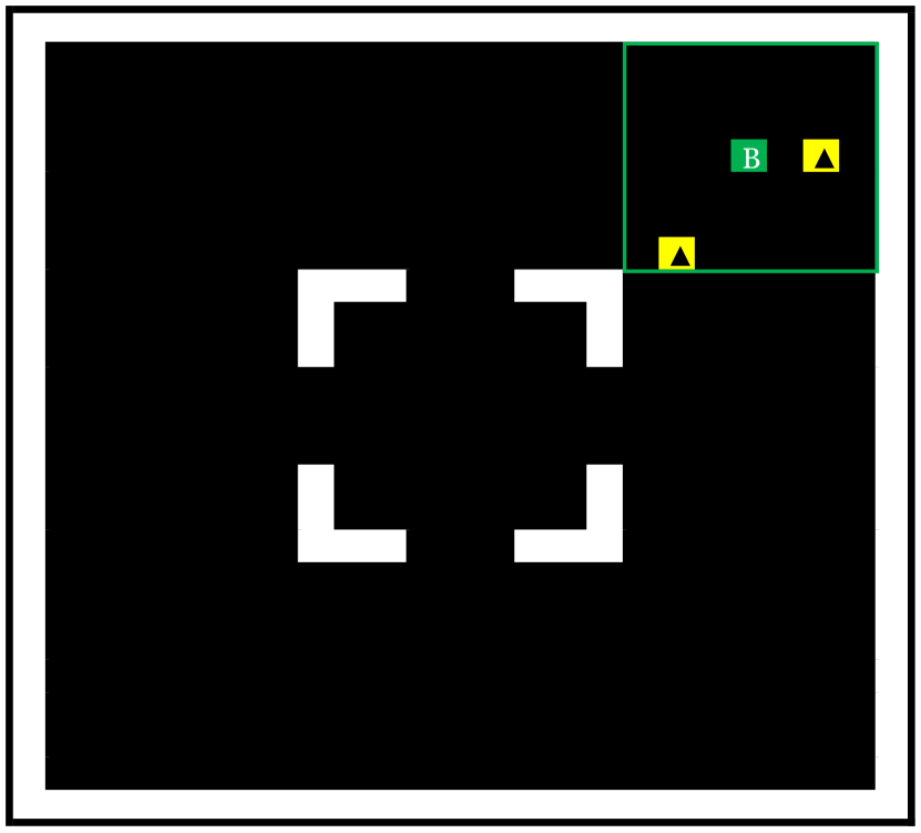
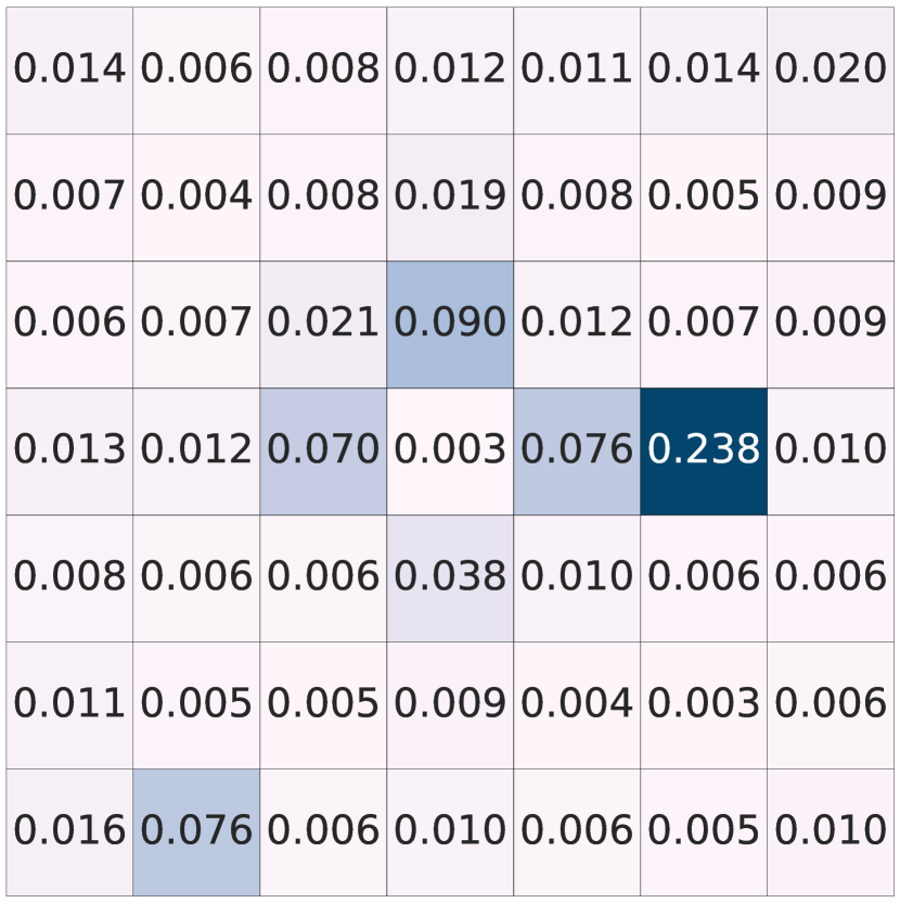
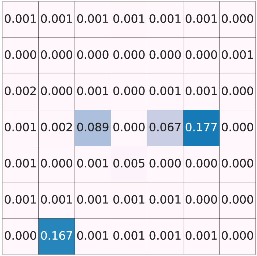
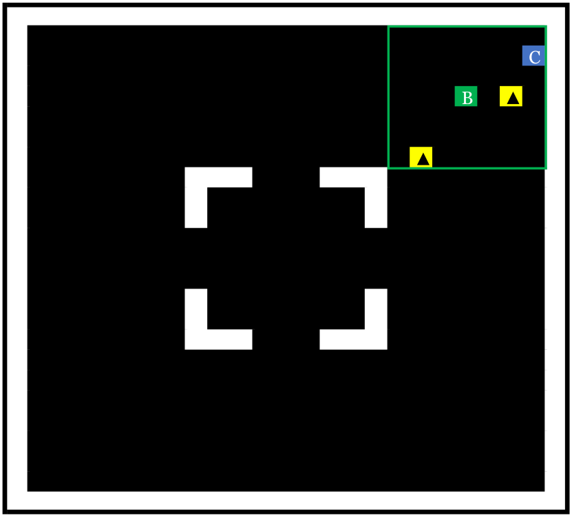
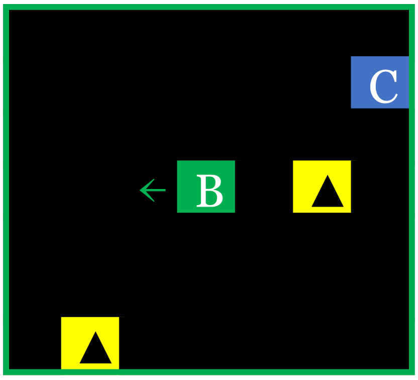
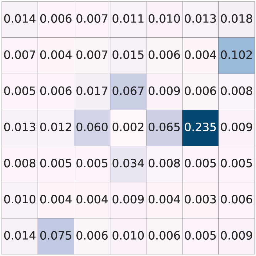
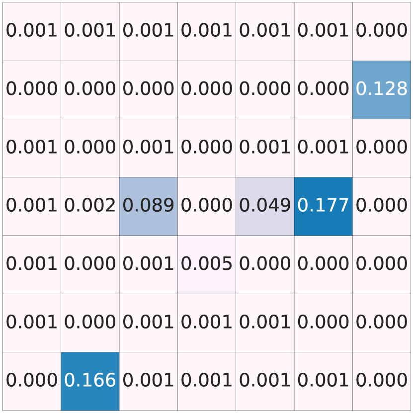
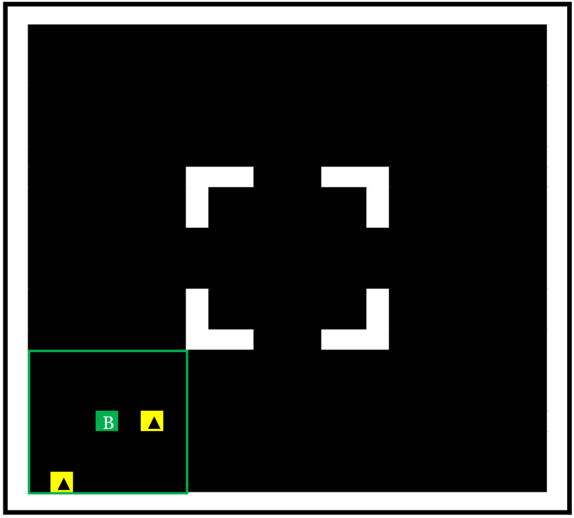
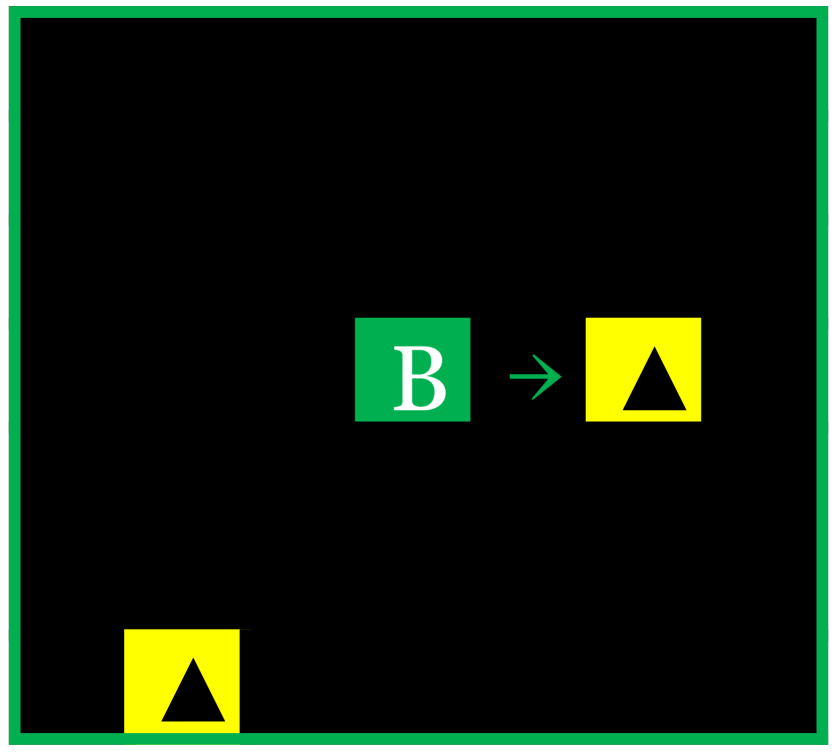
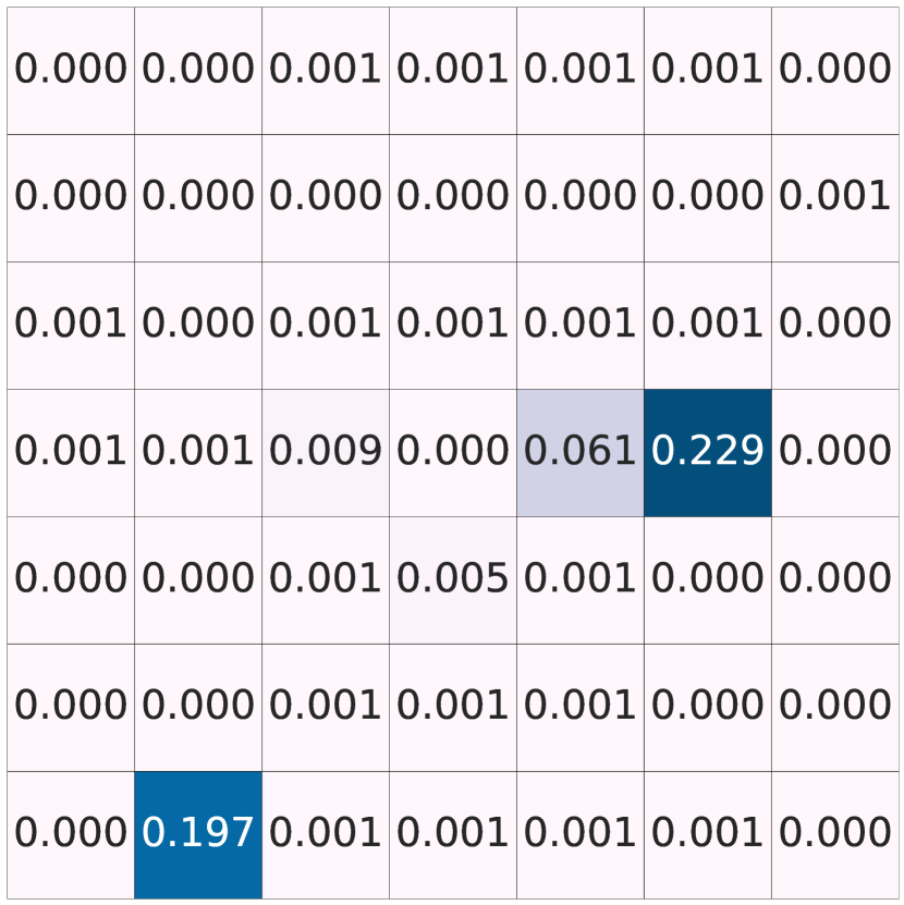
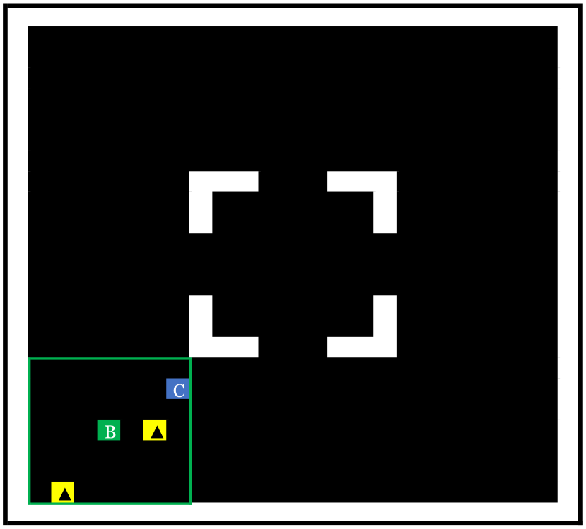
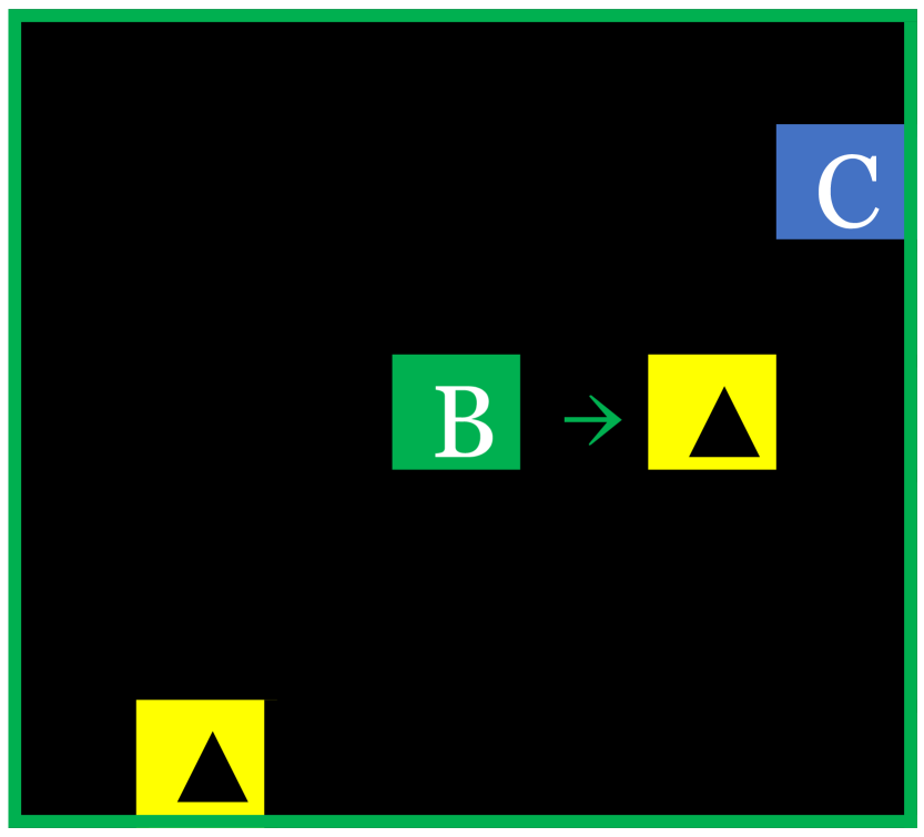
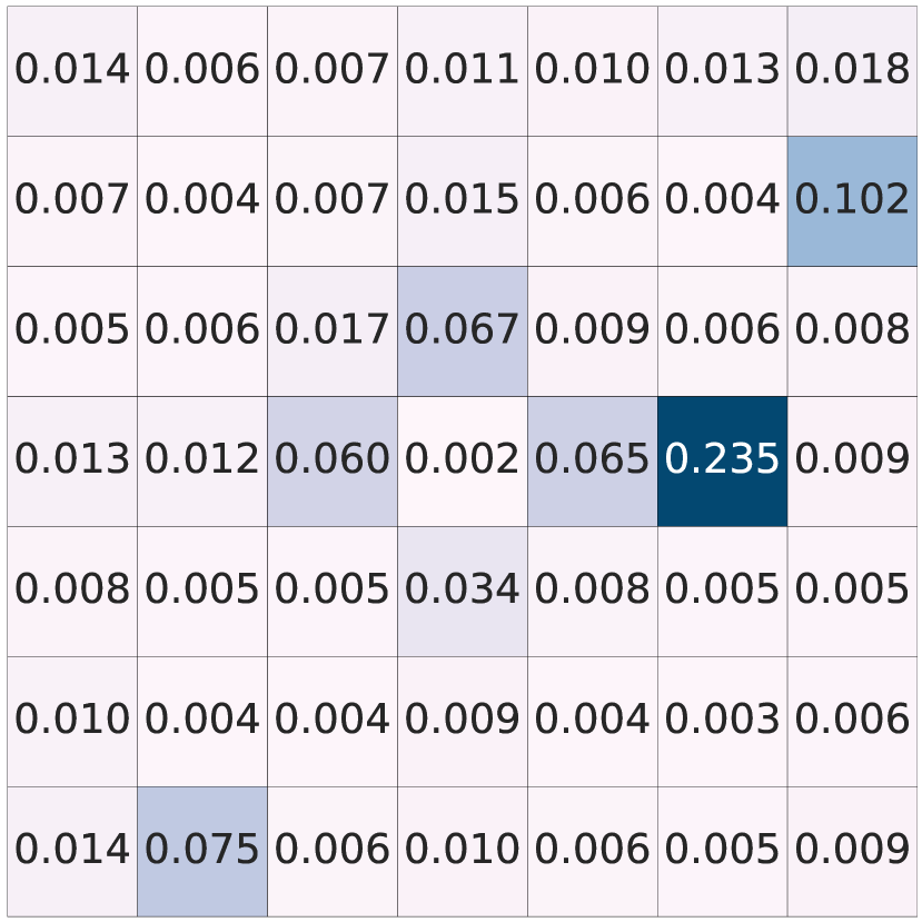
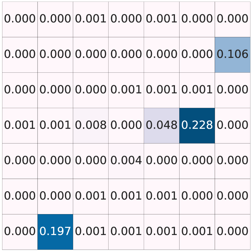
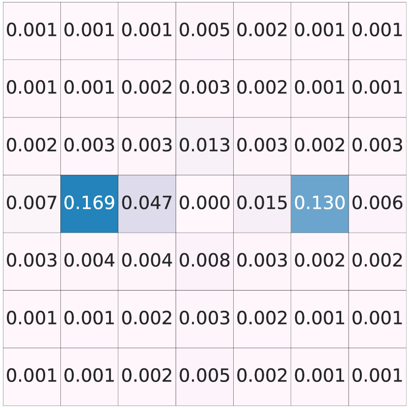
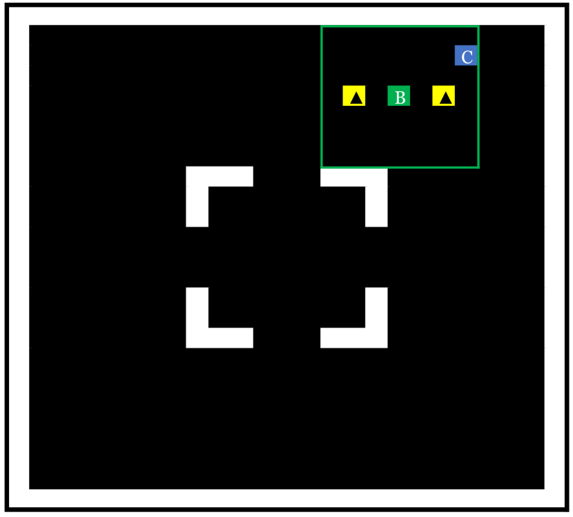
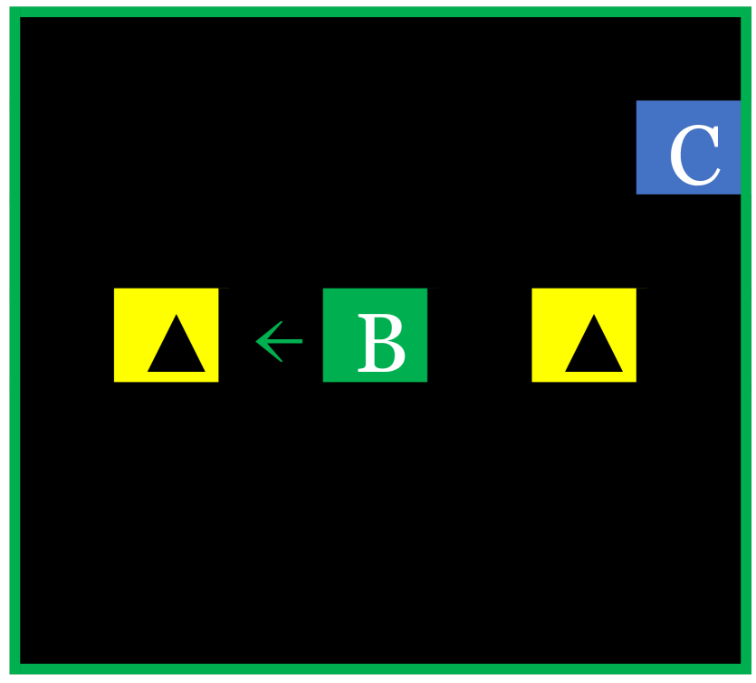
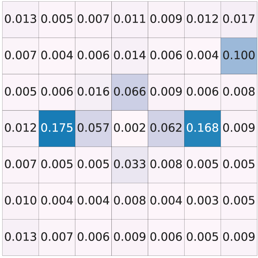
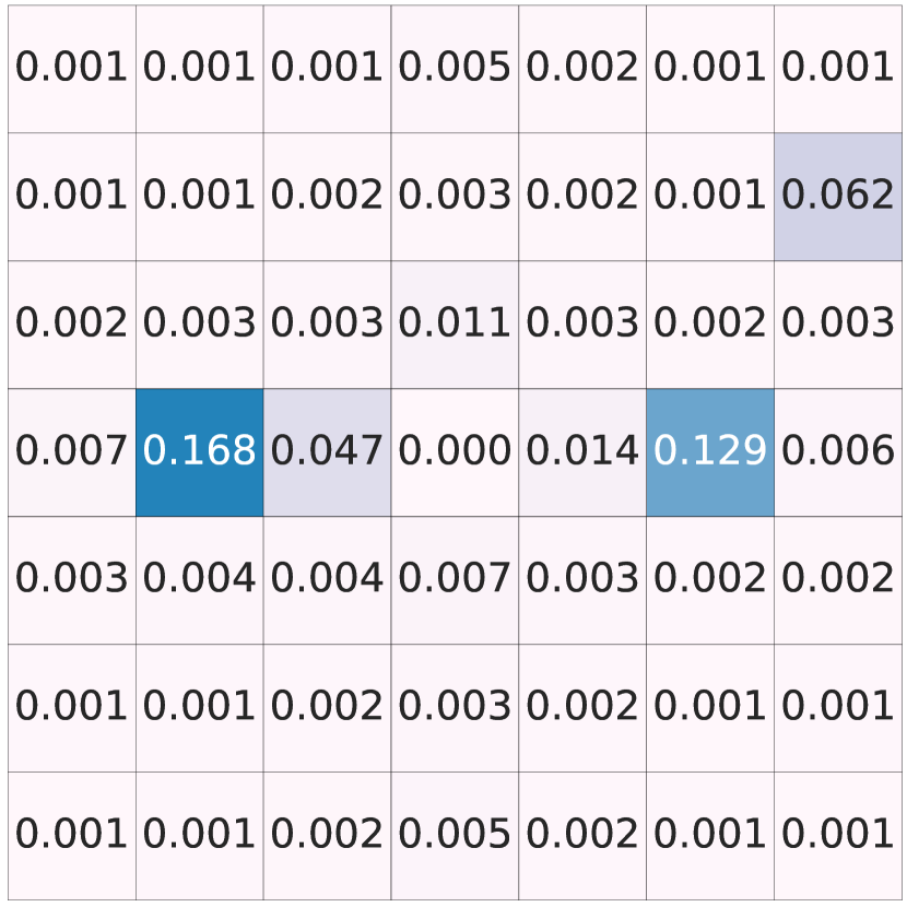
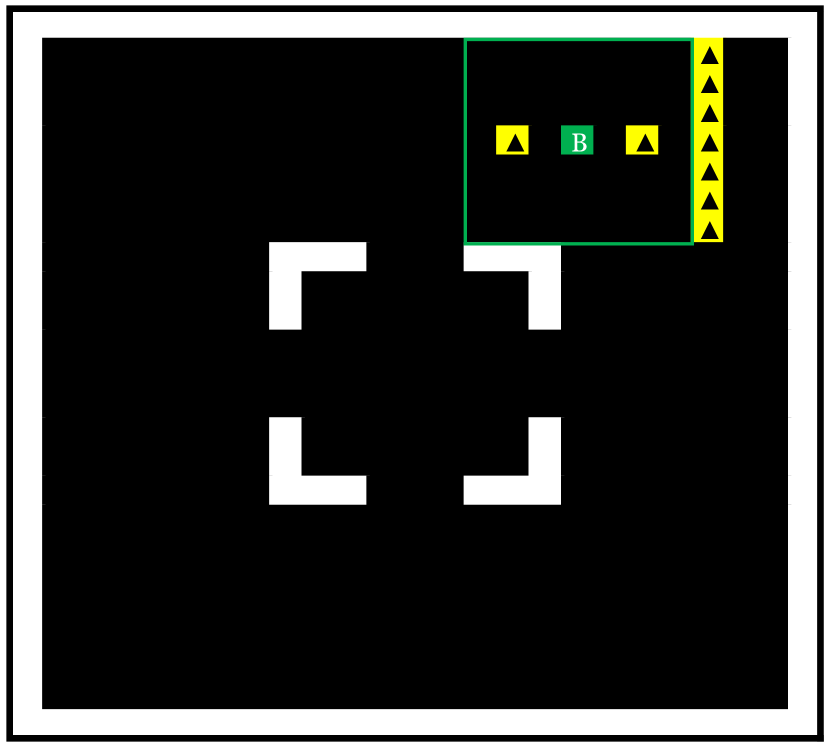
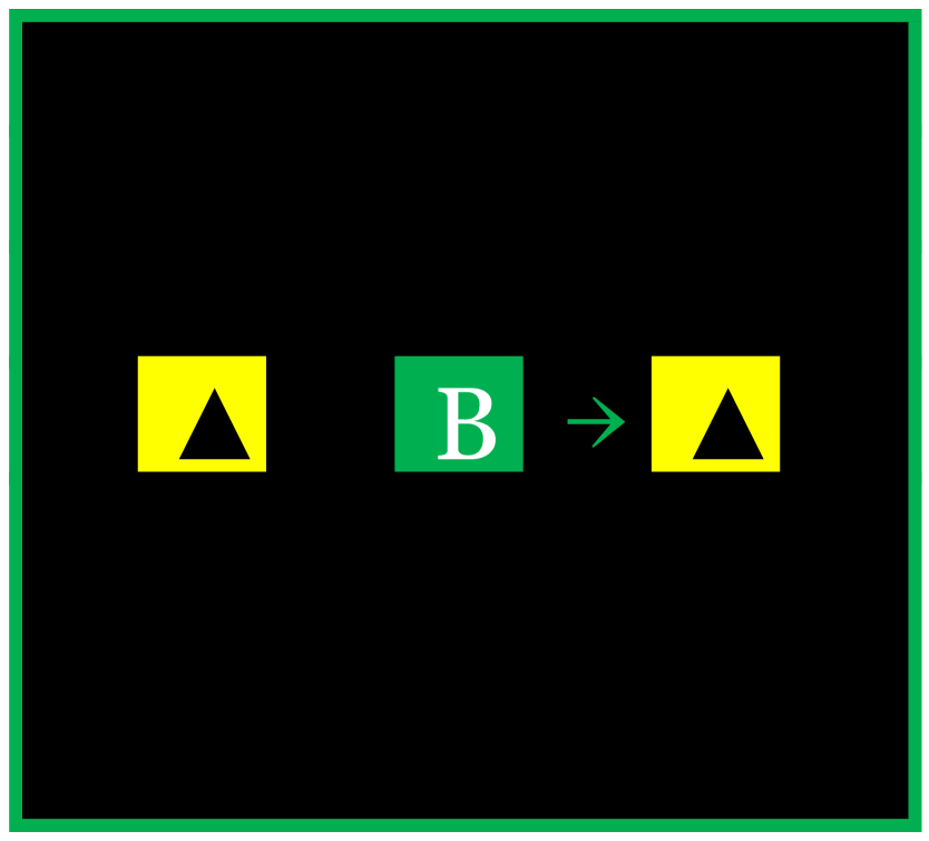
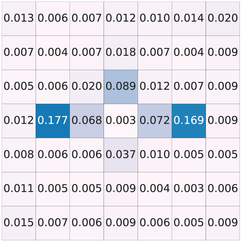
When G pos is available: DA6-DQN agents improved their performance by understanding their global position via the saliency vector. Hence, the way the coordinates vary was analyzed by testing at two different locations: right-up and left-bottom regions ($\Delta$ and $\Theta$). First, how a type B agent behaved with two objects at different distances was observed with/without type C agent located nearby, as depicted in Fig. 4. Each figure shows the global position of the type B agent (top left), the local observation (top right), and the corresponding attention heatmaps of DA3-DQN (bottom left) and DA6-DQN (bottom right) for interpretability comparison. Notably, the attention heatmap of DA3-DQN is generated from the attention weights of the transformer encoder in Fig. 2 without conditional states, while that of DA6-DQN from the local transformer encoder in Fig. 2. The green node in the global position (Fig. 4) is the observing agent itself, and the green square expresses the visible region ($\{R_{\mathrm{X}},R_{\mathrm{Y}}\}=\{7,7\}$). Color in the observation indicates the entities in the environment: white for walls, black for empty, green for observing the type B agent, yellow for the $\blacktriangle$ object, blue for the type C agent. Green arrows in the local observation indicate the orientation of next movement decided by DA6-DQN.

According to Fig. 4 and 4, the type B agent always approaches the closer object by moving toward the right as the closer object attracts more attention than the one farther away ($0.177$ and $0.089$ of DA6-DQN attention when the agent is in the right-upper region $\Delta$ whereas $0.229$ and $0.197$ of DA6-DQN attention when it is in the left-bottom region $\Theta$) regardless of the global position. The attention heatmap by DA3-DQN also puts higher attention on a closer object ($0.238$) than a farther object ($0.076$). However, the attention values are exactly the same in both Fig. 4 and 4 because DA3-X does not consider conditional states.

Interestingly, when the type C agent is located around the closer object (Fig. 4 and 4), the type B agent behaves differently depending on its global position. In the right-upper region $\Delta$ (Fig. 4), the type B agent moves leftward to approach the object farther out by yielding to the type C agent as the attention weight of DA6-DQN is $0.128$. The type B agent understands that the type C agent is aiming at the same target, interpreting it as worth building coordination to avoid competition. In contrast, at the left-bottom region $\Theta$ (Fig. 4), the type B agent assigns an attention weight of DA6-DQN at only $0.106$ to the type C agent and approaches the closer object by moving rightward. The type C agent cannot collect the object in $\Theta$, which is outside its assigned task region according to Table I. The type B agent successfully learned that it is not worth building coordination with the type C agent at the left-bottom region $\Theta$ through training experience. This policy of type B agent is verified from the reduction in attention weight (from $0.128$ to $0.106$ of DA6-DQN attention) on the type C agent at two different locations. Moreover, the behavioral analysis of how the conditional states influence the cooperative behaviors by DA3-X agents becomes very complicated because the attention heatmap by DA3-DQN does not change depending on the global position.

(a) Solo.

(b) With type E agent.

(c) Solo when many objects exist.

(d) With opponent and objects.

Figure 5: Coordination study with G pos + O pos.

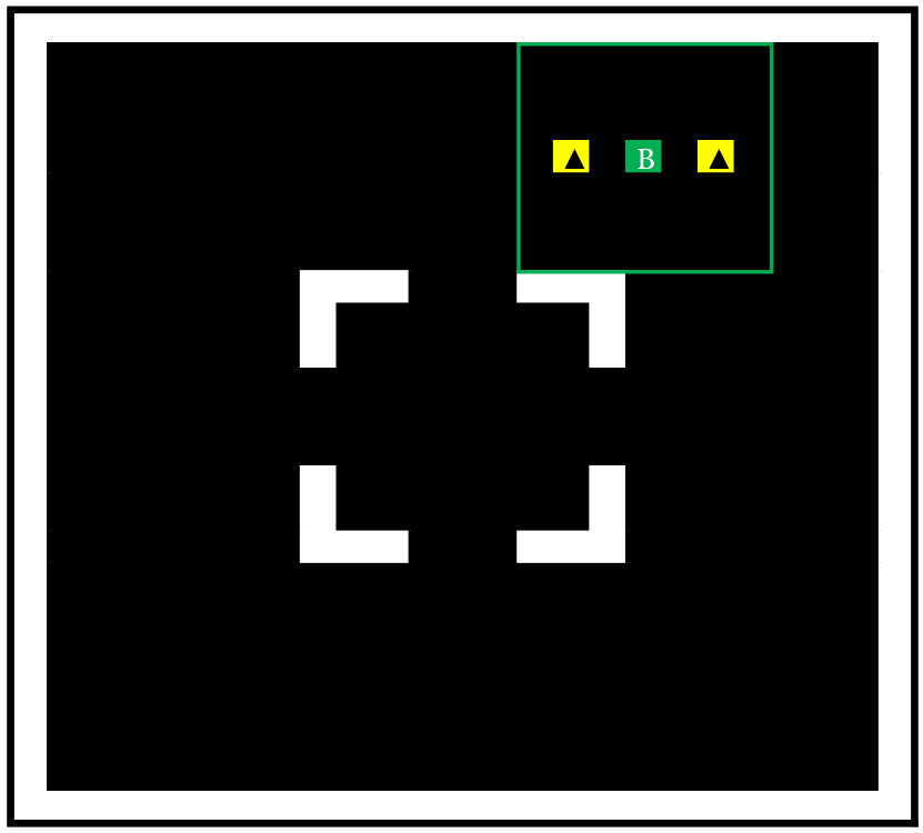
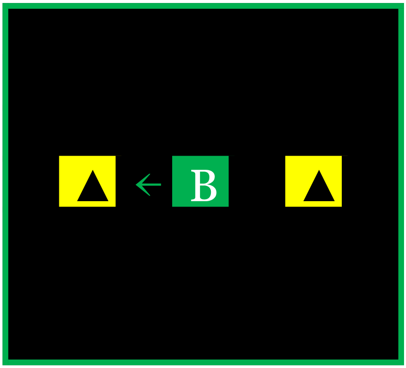
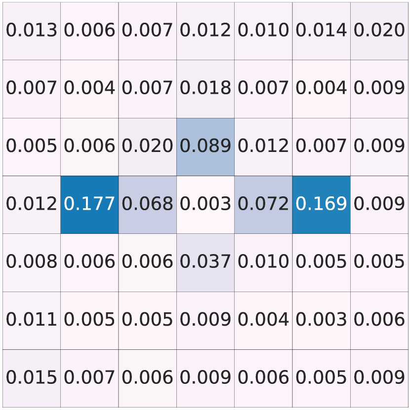
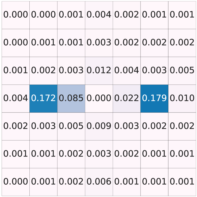
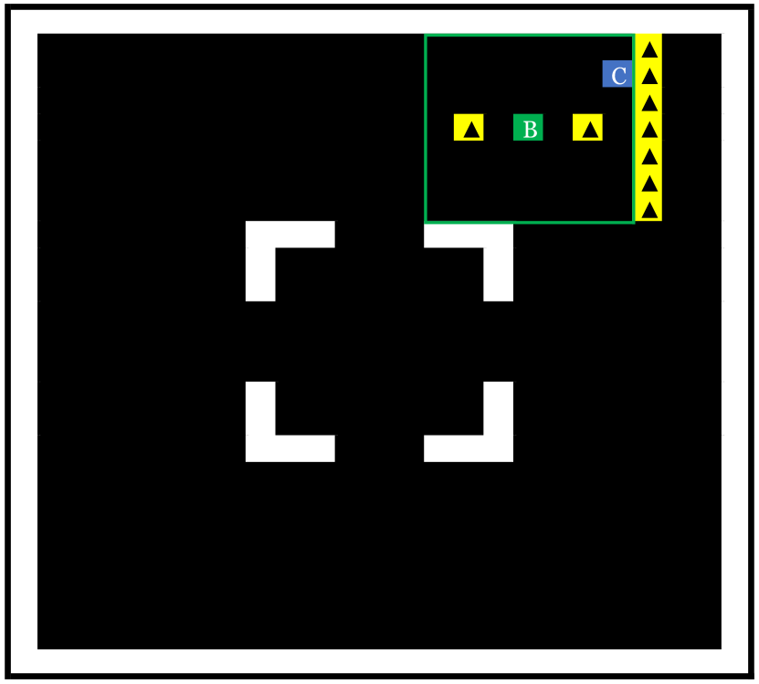
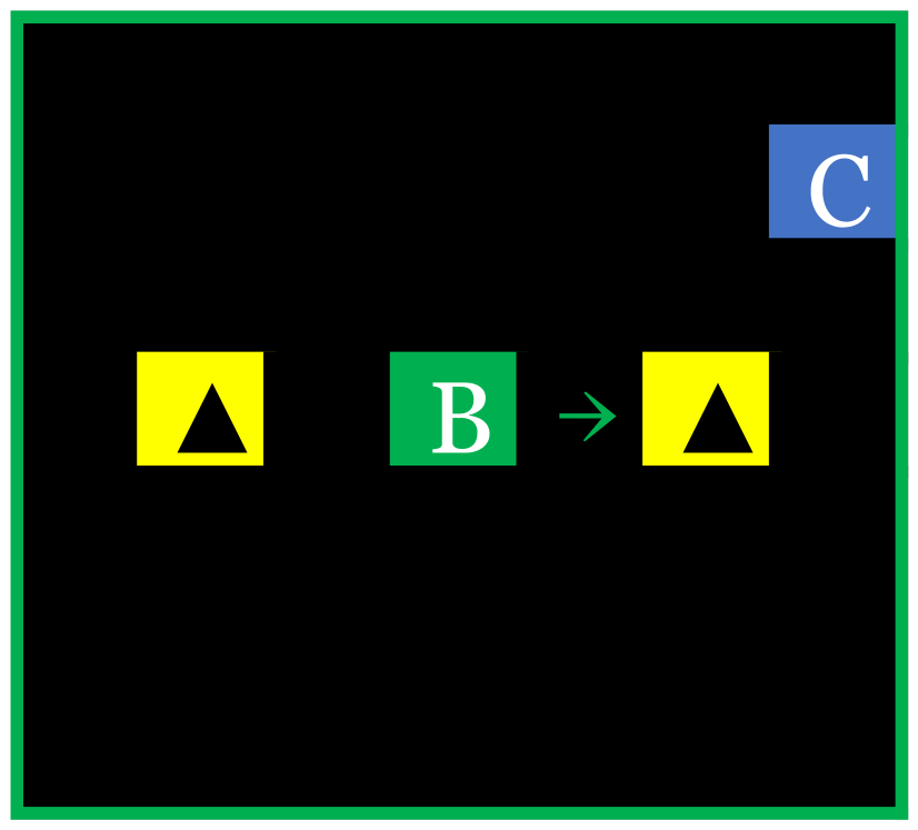
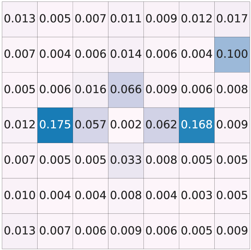
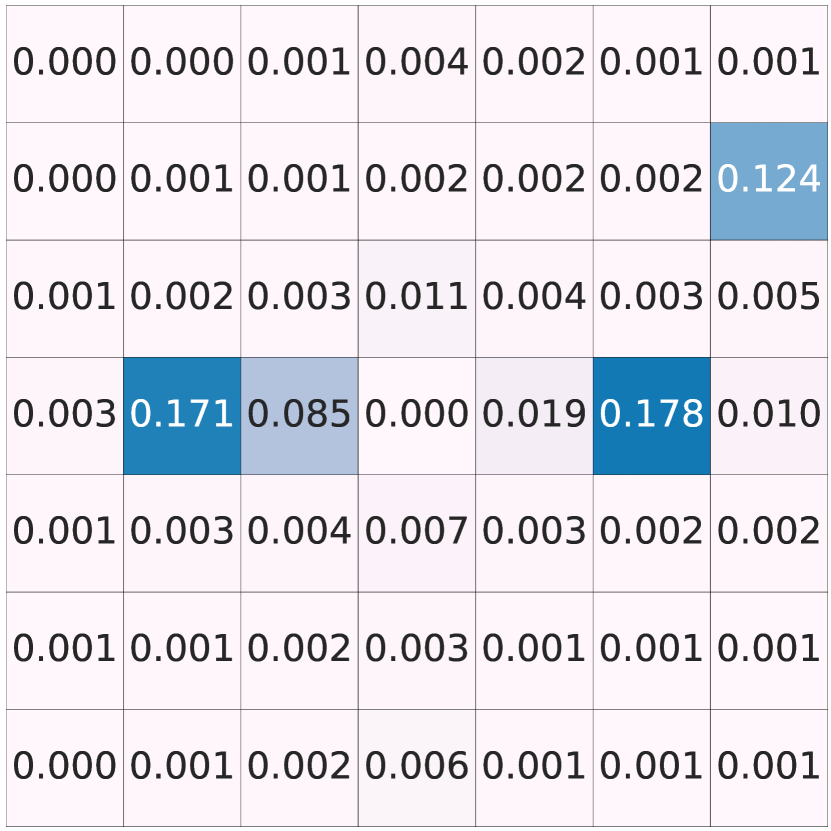
When G pos and O pos are available: According to Fig. 3 and Table II, DA6-X agents achieved even better performance when their global position and objects’ positions were given. Similar to the previous cases, the attention heatmaps of DA3-DQN and DA6-DQN are analyzed to compare and understand the improvement in performance. In this study, two $\blacktriangle$ objects were set at the same distance around the type B agent, and the behavior was analyzed by placing the type C agent close and seven objects outside of the visible range of the type B agent, as illustrated in Fig. 5. The colors in Fig. 5 indicate the same roles as those in Fig. 4.

When the type B agent observes two objects at the same distance in $\Delta$, it moves toward the object on the left, which has a higher attention weight ($0.177$ of DA3-DQN and $0.169$ of DA6-DQN attention) than that of the object on the right ($0.169$ of DA3-DQN and $0.130$ of DA6-DQN attention), as shown in Fig. 5.

The same situation was tested when the type C agent was located inside the visible range (Fig. 5). In this case, the type B agent accorded relatively less attention ($0.100$ of DA3-DQN and $0.062$ of DA6-DQN attention) to the type C agent and moved toward the left object. This behavior is reasonable because the type B agent always intended to collect the left object and the existence of the type C agent on the right did not affect its policy, as shown in the attention heatmap.

Seven objects were added at four units to the right of the type B agent to examine how DA6-IQN agents leverage reusing the saliency vector, which represents G pos and O pos conditions. Interestingly, the type B agent places a high attention weight on the right object ($0.179$ of DA6-DQN attention) and lower attention on the left object ($0.172$ of DA6-DQN attention) after considering the location of seven objects outside of the visible range, as shown in Fig. 5. The agent then moved right to approach more objects. It is verified that DA6-IQN agents successfully understand the approximate locations of other objects outside their vision from the saliency vector and appropriately build efficient strategies.

Finally, the behavior of the type B agent was tested when the type C agent was around and seven objects were located on the right. According to the attention heatmap in Fig. 5, the agent placed high attention weights of $0.178$ and $0.124$ on the right object and type C agent, respectively. The type B agent assigned almost twice more DA6-DQN attention to the type C agent after considering the existence of seven objects outside the visible range because the type C agent can be a competitor collecting the same objects. Indeed, the type B agent moved toward objects on the right along with the type C agent and kept locking on the type C agent.

Because DA6-X reuses the saliency vector in CM and local transformer, we can analyze how the conditional states affect the way of obtaining local observation and leads to the coordination. Hence, DA6-X achieves higher interpretability while improving the learning performance, and it can also deal with multiple conditional states, unlike the baseline algorithms.

VI Conclusion and Discussions

In this study, DA6-X was proposed to improve the interpretability of agents by reusing the saliency vector. Experiments were conducted while providing several conditional states for the object collection game to validate the effectiveness of the proposed method. The result quantitatively demonstrates that DA6-X agents successfully build more efficient policies than baseline methods by reusing the saliency vector, which represents the conditional states of the environment. Analysis of the attention heatmaps generated from the attention weights in the local transformer encoder indicated that providing the conditional states impproves the local observation and coordination strategy of agents and the decision-making process, which had been unknown because of the black-box issue.

This work can be extended to a continuous environment beyond the object collection game. The coordination study of DA6-X agents in a different environment may be in high demand for a better understanding of MADRL and XRL. In addition, the learning performance may improve by replacing transformer encoders in DA6-X with an alternative transformer encoder, such as TAFA introduced by [30] or GTrXL [19].

Our approach may still have limitations in evaluating the interpretability of agents quantitatively. In this work, the mechanism of DA6-X agents observing the environment was introduced via attention heatmaps, qualitatively demonstrating their explainability in several situations. The lack of quantitative evaluation on the explainability may be fatal in critical applications, such as self-driving systems, as in these systems high safety and algorithmic accountability need to be ensured. Therefore, our next research step is to quantitatively examine the transparency of agents’ decision-making process via attention heatmaps.

References

- [1] Lili Chen, Kevin Lu, Aravind Rajeswaran, Kimin Lee, Aditya Grover, Misha Laskin, Pieter Abbeel, Aravind Srinivas, and Igor Mordatch. Decision transformer: Reinforcement learning via sequence modeling. Advances in neural information processing systems, 34, 2021.
- [2] Jinyoung Choi, Beom-Jin Lee, and Byoung-Tak Zhang. Multi-focus attention network for efficient deep reinforcement learning, 2017.
- [3] Will Dabney, Georg Ostrovski, David Silver, and Remi Munos. Implicit quantile networks for distributional reinforcement learning. In Jennifer Dy and Andreas Krause, editors, Proceedings of the 35th International Conference on Machine Learning, volume 80 of Proceedings of Machine Learning Research, pages 1096–1105. PMLR, 10–15 Jul 2018.
- [4] Alexey Dosovitskiy, Lucas Beyer, Alexander Kolesnikov, Dirk Weissenborn, Xiaohua Zhai, Thomas Unterthiner, Mostafa Dehghani, Matthias Minderer, Georg Heigold, Sylvain Gelly, Jakob Uszkoreit, and Neil Houlsby. An image is worth 16x16 words: Transformers for image recognition at scale. In International Conference on Learning Representations, 2021.
- [5] Matteo Hessel, Joseph Modayil, Hado van Hasselt, Tom Schaul, Georg Ostrovski, Will Dabney, Dan Horgan, Bilal Piot, Mohammad Azar, and David Silver. Rainbow: Combining improvements in deep reinforcement learning. Proceedings of the AAAI Conference on Artificial Intelligence, 32(1), Apr. 2018.
- [6] Shariq Iqbal and Fei Sha. Actor-attention-critic for multi-agent reinforcement learning. In Kamalika Chaudhuri and Ruslan Salakhutdinov, editors, Proceedings of the 36th International Conference on Machine Learning, volume 97 of Proceedings of Machine Learning Research, pages 2961–2970. PMLR, 09–15 Jun 2019.
- [7] Rahul Radhakrishnan Iyer, Yuezhang Li, Huao Li, Michael Lewis, Ramitha Sundar, and Katia P. Sycara. Transparency and explanation in deep reinforcement learning neural networks. Proceedings of the 2018 AAAI/ACM Conference on AI, Ethics, and Society, 2018.
- [8] Z. Juozapaitis, A. Koul, A. Fern, M. Erwig, and F. Doshi-Velez. Explainable reinforcement learning via reward decomposition. In in proceedings at the International Joint Conference on Artificial Intelligence. A Workshop on Explainable Artificial Intelligence., 2019.
- [9] Dennis Lee, Natasha Jaques, Chase Kew, Jiaxing Wu, Douglas Eck, Dale Schuurmans, and Aleksandra Faust. Joint attention for multi-agent coordination and social learning, 2021.
- [10] Jiachen Li, Fan Yang, Masayoshi Tomizuka, and Chiho Choi. Evolvegraph: Multi-agent trajectory prediction with dynamic relational reasoning. In Proceedings of the Neural Information Processing Systems (NeurIPS), 2020.
- [11] Max Guangyu Li, Bo Jiang, Hao Zhu, Zhengping Che, and Yan Liu. Generative attention networks for multi-agent behavioral modeling. In AAAI, 2020.
- [12] Timothy P. Lillicrap, Jonathan J. Hunt, Alexander Pritzel, Nicolas Manfred Otto Heess, Tom Erez, Yuval Tassa, David Silver, and Daan Wierstra. Continuous control with deep reinforcement learning. CoRR, abs/1509.02971, 2016.
- [13] Ryan Lowe, Yi Wu, Aviv Tamar, Jean Harb, Pieter Abbeel, and Igor Mordatch. Multi-agent actor-critic for mixed cooperative-competitive environments. In Proceedings of the 31st International Conference on Neural Information Processing Systems, NIPS’17, pages 6382–6393, Red Hook, NY, USA, 2017. Curran Associates Inc.
- [14] Xueguang Lyu, Yuchen Xiao, Brett Daley, and Chris Amato. Contrasting centralized and decentralized critics in multi-agent reinforcement learning. ArXiv, abs/2102.04402, 2021.
- [15] Yuki Miyashita and Toshiharu Sugawara. Analysis of coordinated behavior structures with multi-agent deep reinforcement learning. Applied Intelligence, 51(2):1069–1085, February 2021. Funding Information: This work was partly supported by JSPS KAKENHI Grant Number 17KT0044. Publisher Copyright: © 2020, The Author(s).
- [16] Volodymyr Mnih, Koray Kavukcuoglu, David Silver, Andrei A. Rusu, Joel Veness, Marc G. Bellemare, Alex Graves, Martin Riedmiller, Andreas K. Fidjeland, Georg Ostrovski, Stig Petersen, Charles Beattie, Amir Sadik, Ioannis Antonoglou, Helen King, Dharshan Kumaran, Daan Wierstra, Shane Legg, and Demis Hassabis. Human-level control through deep reinforcement learning. Nature, 518(7540):529–533, 2015.
- [17] Yoshinari Motokawa and Toshiharu Sugawara. MAT-DQN: Toward interpretable multi-agent deep reinforcement learning for coordinated activities. In Artificial Neural Networks and Machine Learning - ICANN 2021: 30th International Conference on Artificial Neural Networks, Bratislava, Slovakia, September 14-17, 2021, Proceedings, Part IV, pages 556–567, 2021.
- [18] Yoshinari Motokawa and Toshiharu Sugawara. Distributed multi-agent deep reinforcement learning for robust coordination against noise. In 2022 International Joint Conference on Neural Networks (IJCNN), pages 1–8, 2022.
- [19] Emilio Parisotto, Francis Song, Jack Rae, Razvan Pascanu, Caglar Gulcehre, Siddhant Jayakumar, Max Jaderberg, Raphael Lopez Kaufman, Aidan Clark, Seb Noury, et al. Stabilizing transformers for reinforcement learning. In International Conference on Machine Learning, pages 7487–7498. PMLR, 2020.
- [20] P. Parnika, Raghuram Bharadwaj Diddigi, Sai Koti Reddy Danda, and Shalabh Bhatnagar. Attention actor-critic algorithm for multi-agent constrained co-operative reinforcement learning. In Proceedings of the 20th International Conference on Autonomous Agents and MultiAgent Systems, AAMAS ’21, pages 1616–1618, Richland, SC, 2021. International Foundation for Autonomous Agents and Multiagent Systems.
- [21] Erika Puiutta and Eric M. S. P. Veith. Explainable reinforcement learning: A survey. In Andreas Holzinger, Peter Kieseberg, A Min Tjoa, and Edgar Weippl, editors, Machine Learning and Knowledge Extraction, pages 77–95, Cham, 2020. Springer International Publishing.
- [22] Martin L. Puterman. Markov Decision Processes: Discrete Stochastic Dynamic Programming. John Wiley & Sons, Inc., USA, 1st edition, 1994.
- [23] John Schulman, Filip Wolski, Prafulla Dhariwal, Alec Radford, and Oleg Klimov. Proximal policy optimization algorithms. CoRR, abs/1707.06347, 2017.
- [24] Ken Smith, Yuki Miyashita, and Toshiharu Sugawara. Analysis of coordination structures of partially observing cooperative agents by multi-agent deep q-learning. In PRIMA 2020: Principles and Practice of Multi-Agent Systems: 23rd International Conference, Nagoya, Japan, November 18-20, 2020, Proceedings, pages 150–164, 2020.
- [25] Mukund Sundararajan, Ankur Taly, and Qiqi Yan. Axiomatic attribution for deep networks. In Proceedings of the 34th International Conference on Machine Learning - Volume 70, ICML’17, pages 3319–3328. JMLR.org, 2017.
- [26] Ashish Vaswani, Noam Shazeer, Niki Parmar, Jakob Uszkoreit, Llion Jones, Aidan N Gomez, Ł ukasz Kaiser, and Illia Polosukhin. Attention is all you need. In I. Guyon, U. V. Luxburg, S. Bengio, H. Wallach, R. Fergus, S. Vishwanathan, and R. Garnett, editors, Advances in Neural Information Processing Systems, 2017.
- [27] Wenguan Wang, Jianbing Shen, Xiankai Lu, Steven C. H. Hoi, and Haibin Ling. Paying attention to video object pattern understanding. IEEE Transactions on Pattern Analysis and Machine Intelligence, 43(7):2413–2428, 2021.
- [28] Vinicius Zambaldi, David Raposo, Adam Santoro, Victor Bapst, Yujia Li, Igor Babuschkin, Karl Tuyls, David Reichert, Timothy Lillicrap, Edward Lockhart, Murray Shanahan, Victoria Langston, Razvan Pascanu, Matthew Botvinick, Oriol Vinyals, and Peter Battaglia. Deep reinforcement learning with relational inductive biases. In International Conference on Learning Representations, 2019.
- [29] Matthew D. Zeiler and Rob Fergus. Visualizing and understanding convolutional networks. In David Fleet, Tomas Pajdla, Bernt Schiele, and Tinne Tuytelaars, editors, Computer Vision – ECCV 2014, pages 818–833, Cham, 2014. Springer International Publishing.
- [30] Qiyuan Zhang, Xiaoteng Ma, Yiqin Yang, Chenghao Li, Jun Yang, Yu Liu, and Bin Liang. Learning to discover task-relevant features for interpretable reinforcement learning. IEEE Robotics and Automation Letters, 6(4):6601–6607, 2021.