The effect of estimating prevalences on the population-wise error rate

Abstract

The population-wise error rate (PWER) is a type I error rate for clinical trials with multiple target populations. In such trials, one treatment is tested for its efficacy in each population. The PWER is defined as the probability that a randomly selected, future patient will be exposed to an inefficient treatment based on the study results. The PWER can be understood and computed as an average of strata specific family-wise error rates and involves the prevalences of these strata. A major issue of this concept is that the population prevalences needed to determine this average are usually not known in practice, so that the PWER cannot be directly controlled. Instead, one could use an estimator of the prevalences based on the given sample, like their maximum-likelihood estimator. In this paper we show in simulations that this does not substantially inflate the true PWER. We differentiate between the expected PWER, which is almost perfectly controlled, and study-specific values of the PWER which are conditioned to given sample sizes and vary within a narrow range. Thereby, we consider up to eight different overlapping patient populations and moderate to large sample sizes.

Keywords Family-wise error rate  $\cdot$ Multinomial distribution  $\cdot$ Multiple testing  $\cdot$ Population-wise error rate  $\cdot$ Relative prevalences

1 Introduction

Many clinical trials in personalised medicine examine multiple hypotheses, each about the efficacy of a medical treatment in a patient population defined by certain inclusion or exclusion criteria. If some of these populations overlap, taking a false test decision may affect more than one population. In this case, type I error control should be adjusted for multiplicity. For this purpose, Brannath et al. (2023) introduced the population-wise error rate (PWER), a multiple type I error rate which is adapted to clinical studies with overlapping populations. It has the advantage of being more liberal than the family-wise error rate and thus enabling greater power. This is particularly useful when examining rare diseases, when only small sample sizes are available. The PWER gives the average probability that a randomly selected patient from the overall population will receive an inefficient treatment. For calculating it, the overall population is partitioned into disjoint strata, each containing individuals affected by the same test decisions. For each stratum, the respective multiple type I error probability is then weighted by its relative prevalence, i.e. the proportion of the stratum in the total population. In practice, however, the relative prevalences are often not known and must be estimated from the study sample. One appropriate way to do this is to use the maximum-likelihood-estimator from the multinomial distribution. This paper aims to examine whether the use of this estimator inflates the true PWER and to which extent. To this end, we will carry out simulations in which the relative prevalences will be estimated and used for the calculation of the rejection boundaries in order to control the estimated PWER at the pre-specified level. We will then compare the true PWER (using the true prevalences) to this significance level.

We start this paper with the formal definition of the PWER (section 2). In section 3, we construct the test statistics used to handle the population-wise testing problems. We will primarily consider the situation where different treatments are tested in the populations, which is done, for example, in umbrella trials where the populations are defined by certain biomarkers that can appear in a certain type of cancer. The presentation of the simulations and their results is done in sections 4.1-4.5. In section 4.6, we will also consider the maximal strata-wise error probabilites resulting from PWER-control, to find out whether these will not become too large by not directly controlling the FWER but the PWER. Brannath et al. (2023) have already specified several upper limits, which are somewhat rough and can often be improved by the simulated values. In addition we will introduce an adjustment of the PWER in section 4.7 that could be made when, by chance, no patients are recruited from a stratum. The PWER would then be reduced in order to control for multiplicity in this stratum as well. The paper ends with a discussion in section 5.

2 The population-wise error rate (PWER)

In this section we first recall the formal definition of the PWER from Brannath et al. (2023) and present a result on least favourable parameter configurations for the PWER which will be used in the calculation of the rejection boundaries for PWER control.

2.1 Definition

Let $\mathcal{P}_{1},\dots,\mathcal{P}_{m}$ be the sets representing the given patient populations. They may, in particular, be overlapping. For every $i\in I=\{1,\dots,m\}$ we want to test a certain treatment $T_{i}$ in the population $\mathcal{P}_{i}$. Therefore we consider the null hypothesis $H_{i}\colon\theta_{i}\leq 0$, where $\theta_{i}=\theta(\mathcal{P}_{i},T_{i})\in\mathbb{R}$ denotes the efficacy of $T_{i}$ in comparison to a control treatment $C$ in the population $\mathcal{P}_{i}$. We now partition the overall population $\mathcal{P}=\cup_{i=1}^{m}\mathcal{P}_{i}$ into the (disjoint) subpopulations that include all individuals affected by the same treatments. This is achieved by defining the strata $\mathcal{P}_{J}\coloneqq\left(\cap_{j\in J}\mathcal{P}_{j}\right)\backslash\left(\cup_{k\in I\setminus J}\mathcal{P}_{k}\right)$ for all $J\subseteq I$. Figure 1 illustrates the resulting partition in the case of $m=3$ overlapping populations. For each stratum $\mathcal{P}_{J}$ we denote its relative prevalence among $\mathcal{P}$ by $\pi_{J}$. Since the prevalences are usually unknown in practice, we will later propose how to estimate them. The population-wise error rate of the multiple testing problem is defined by

$$\text{PWER}=\sum_{J\subseteq I}\pi_{J}\text{P}(\text{falsely reject any $H_{j}$ with $j\in J$}).$$

So it gives the average probability of committing at least one type I error that would concern the individuals in $\mathcal{P}$. The PWER is more liberal than the family-wise-error-rate (FWER), i.e. it fulfils $\text{PWER}\leq\text{FWER}$ (see Brannath et al. (2023)).

Figure 1: Partition of $m=3$ overlapping populations

In this paper we suppose that each hypothesis $H_{i}$ is tested in a right-tailed test, using the test statistic $Z_{i}$ and the common critical value $c$, so that the PWER equals to

$$\text{PWER}_{\theta}=\sum_{J\subseteq I}\,\pi_{J}\,\text{P}_{\theta}\left(\bigcup_{j\in J\cap I_{0}(\theta)}\{Z_{j}>c\}\right).$$

It depends on the vector $\theta=(\theta_{1},\dots,\theta_{m})$ of the true efficacies, and on the corresponding true null hypotheses which are indexed in $I_{0}(\theta)=\{i\in I:\theta_{i}\leq 0\}$.

2.2 Least favourable parameter configurations

Under two additional assumptions it can be shown that the null vector $0\in\mathbb{R}^{m}$ is a worst case parameter $\theta$ for which the PWER attains its maximum. The first condition is the subset pivotality assumption (see Westfall and Young (1993); Dickhaus (2014)), which states that the multivariate distributions of the vectors $(Z_{j})_{j\in J\cap I_{0}(\theta)}$ do not depend on the truth or falsity of those hypotheses they are not relevant for. It is formally described by

$$\forall\,J\subseteq I,J\neq\emptyset:\forall\,\theta\in H_{J}:\exists\,\theta^{*}\in H_{I}:\text{P}_{\theta}^{\max_{j\in J}Z_{j}}=\text{P}_{\theta^{*}}^{\max_{j\in J}Z_{j}},$$ (1)

where $H_{J}\coloneqq\bigcap_{j\in J}H_{j}\subseteq\mathbb{R}^{m}$, $J\subseteq I$, and $\text{P}_{\theta}^{\max_{j\in J}Z_{j}}$ denotes the distribution of $\max_{j\in J}Z_{j}$ in dependence of the parameter $\theta$. The second assumption is stochastic monotonicity of the subvectors $(Z_{j})_{j\in J}$, stating that

$$\forall\,J\subseteq I,J\neq\emptyset:\forall\,\theta,\theta^{\prime}\in H_{I},\theta\leq\theta^{\prime}:\text{P}_{\theta}\left(\max_{j\in J}Z_{j}>c\right)\leq\text{P}_{\theta^{\prime}}\left(\max_{j\in J}Z_{j}>c\right).$$ (2)

Here the relation $\theta\leq\theta^{\prime}$ is meant component-wise.

Theorem 1

Under conditions (1) and (2) one obtains $\sup_{\theta\in\mathbb{R}^{m}}\text{PWER}_{\theta}=\text{PWER}_{\theta^{*}}$ for $\theta^{*}=0\in\mathbb{R}^{m}$.

The proof of this can be found in appendix A. We call every $\theta^{*}$ fulfilling the equation from theorem 1 a least favourable parameter configuration (LFC) for the PWER. The existence of a LFC is very useful for controlling the PWER at a given significance level $\alpha\in(0,1)$. This can then be achieved by choosing the smallest critical value $c$ that satisfies $\text{PWER}_{\theta^{*}}(c)\leq\alpha$.

3 Choice of the test statistics

We now want to construct the vector of test statistics $Z=(Z_{i})_{i\in I}$ in order to conduct the multiple test. We consider the case where different treatments are tested, i.e. $T_{i}\neq T_{j}$ for $i\neq j$. Suppose that a sample of $N$ patients is given, in which $n_{J}$ patients belong to the stratum $\mathcal{P}_{J}$, for every $J\subseteq I$. We follow the approach proposed by Hillner (2021), but replace the true prevalences used there by the given sample sizes.

For every $i\in I$, let $\mu_{T_{i}}^{i}\in\mathbb{R}$ be the mean efficacy of $T_{i}$ in the population $\mathcal{P}_{i}$ and let $\mu_{C}^{i}\in\mathbb{R}$ be the mean efficacy of the control $C$ in $\mathcal{P}_{i}$. Then we have $\theta_{i}=\mu_{T_{i}}^{i}-\mu_{C}^{i}$. Additionally, for every $J\subseteq I$ we define the efficacies $\mu_{T_{j}}^{J}\in\mathbb{R}$ of $T_{j}$ in $\mathcal{P}_{J}$ (for all $j\in J$) and $\mu_{C}^{J}\in\mathbb{R}$ of $C$ in $\mathcal{P}_{J}$, which fulfil

$$\mu_{T_{i}}^{i}=\sum_{J\subseteq I:\,i\in J}\frac{\pi_{J}}{\pi_{i}}\mu_{T_{i}}^{J}\quad\text{and}\quad\mu_{C}^{i}=\sum_{J\subseteq I:\,i\in J}\frac{\pi_{J}}{\pi_{i}}\mu_{C}^{J},$$

where $\pi_{i}$ denotes the sum of all $\pi_{J}$ with $i\in J$ (and equals the prevalence of $\mathcal{P}_{i}$). In every stratum $\mathcal{P}_{J}$ we randomize the patients to the treatments evenly, such that $n_{J}/(|J|+1)$ patients get the treatments $T_{j}$ (for all $j\in J$) and $C$, respectively. We will ignore that this could be an uneven number, because this will not be a constraint in the simulations of section 4.

3.1 Normal distribution model with homogeneous, known variances

In every stratum $\mathcal{P}_{J}$, let us represent the measured effects of the $T_{j}$ (with $j\in J$) and $C$ through the normally distributed random variables $X^{J}_{T_{j},k}\sim\text{N}(\mu_{T_{j}}^{J},\sigma^{2})$ and $X_{C,k}^{J}\sim\text{N}(\mu_{C}^{J},\sigma^{2})$, for $k=1,\dots,n_{J}/(|J|+1)$. The variance $\sigma^{2}>0$ is here assumed to be known, and all the observations are assumed to be independent. For every $J$ and for every treatment $B\in\mathcal{T}_{J}\coloneqq\{T_{j}:j\in J\}\cup\{C\}$ we define the strata-wise arithmetic mean $\bar{X}_{B}^{J}\coloneqq\frac{1}{n_{J}/(|J|+1)}\sum_{k=1}^{n_{J}/(|J|+1)}X_{B,k}^{J}$. Then we can estimate the true effects $\mu_{T_{i}}^{i}$ and $\mu_{C}^{i}$ through

$$\hat{\mu}_{T_{i}}^{i}\coloneqq\sum_{J\subseteq I:\,i\in J}\frac{n_{J}}{n_{i}}\bar{X}_{T_{i}}^{J}\quad\text{and}\quad\hat{\mu}_{C}^{i}\coloneqq\sum_{J\subseteq I:\,i\in J}\frac{n_{J}}{n_{i}}\bar{X}_{C}^{J}.$$

This provides the (standardized) test statistics

$$Z_{i}\coloneqq\frac{\hat{\mu}_{T_{i}}^{i}-\hat{\mu}_{C}^{i}}{\sqrt{\text{Var}\left(\hat{\mu}_{T_{i}}^{i}-\hat{\mu}_{C}^{i}\right)}},\;i\in I.$$

One finds $V_{i}\coloneqq\text{Var}\left(\hat{\mu}_{T_{i}}^{i}-\hat{\mu}_{C}^{i}\right)=\sum_{J\subseteq I:\,i\in J}2n_{J}n_{i}^{-2}(|J|+1)\sigma^{2}.$ The vector $Z=(Z_{i})_{i\in I}$ follows a multivariate normal distribution, for whose parameters $\nu$ and $\Sigma$ we get

$$\nu_{i}=\frac{1}{\sqrt{V_{i}}}\left(\sum_{J\subseteq I:\,i\in J}\frac{n_{J}}{n_{i}}\left(\mu_{T_{i}}^{J}-\mu_{C}^{J}\right)\right)\quad\text{and}\quad\Sigma_{ij}=\frac{\sum_{J\subseteq I:\,i,j\in J}n_{J}(|J|+1)\sigma^{2}}{n_{i}n_{j}\sqrt{V_{i}V_{j}}}$$ (3)

for all $i\neq j$. The variance $\sigma^{2}$ cancels out in the right fraction, so that $\Sigma_{ij}$ is independent from $\sigma^{2}$. In the special case where one single treatment $T$ is tested in all populations, $\Sigma_{ij}$ reduces to $\Sigma_{ij}=\sum_{J\subseteq I:\,i,j\in J}n_{J}/\sqrt{n_{i}n_{j}}$.

We note that in both cases $Z$ fulfills the conditions (1) and (2), so that $\theta=0$ is a LFC for the PWER. Consequently, the maximal PWER can be calculated by

$$\text{PWER}=\sum_{J\subseteq I}\pi_{J}\left(1-\Phi_{\nu_{J},\Sigma_{J}}(c,\dots,c)\right),$$ (4)

where $\Phi$ denotes the cumulative distribution function of the normal distribution, which is restricted to $\nu_{J}\coloneqq(\nu_{j})_{j\in J}$ and $\Sigma_{J}\coloneqq\left(\Sigma_{ij}\right)_{i,j\in J}$.

3.2 Normal distribution model with homogeneous, unknown variances

We now assume the variance $\sigma^{2}$ to be unknown. For every $J\subseteq I$ and $B\in\mathcal{T}_{J}$ an unbiased estimator of $\sigma^{2}$ is given by

$$\hat{\sigma}_{J,B}^{2}=\frac{1}{n_{J}/(|J|+1)-1}\sum_{k=1}^{n_{J}/(|J|+1)}\left(X^{J}_{B,k}-\bar{X}_{B}^{J}\right)^{2}.$$

Let $s\coloneqq\#\{J:J\subseteq I\}=2^{m}-1$ be the number of strata. We use the (also unbiased) composite estimator

$$\hat{\sigma}^{2}=\frac{\sum_{J\subseteq I,\,B\in\mathcal{T}_{J}}(n_{J}/(|J|+1)-1)\hat{\sigma}_{J,B}^{2}}{N-s}$$

to construct the test statistics

$$T_{i}\coloneqq\frac{\hat{\mu}_{T_{i}}^{i}-\hat{\mu}_{C}^{i}}{\sqrt{W_{i}}},\quad\text{with}\quad W_{i}\coloneqq\sum_{J\subseteq I:\,i\in J}2n_{J}n_{i}^{-2}(|J|+1)\hat{\sigma}^{2},\quad i\in I.$$

Similarly to the previous section, the vector $\left(T_{i}\right)_{i\in I}\sim t_{N-s}(\nu^{\prime},\Sigma^{\prime})$ follows a noncentral multivariate $t$-distribution (of type Kshirsagar (1961)) with $N-s$ degrees of freedom. So in this case the PWER can be computed by replacing $\Phi_{\nu,\Sigma}$ with Kshirsagar’s cumulative distribution function $\Psi_{\nu^{\prime},\Sigma^{\prime}}$ using the noncentrality parameter $\nu^{\prime}=\sqrt{N-s}\cdot\nu$ and the scale matrix $\Sigma^{\prime}=\sqrt{N-s}\cdot\Sigma$ in formula (4).

4 Estimation of the population prevalences

The populations $\mathcal{P}_{1},\dots,\mathcal{P}_{m}$ are usually defined by certain inclusion and exclusion criteria and are of infinite size, because they should not only include current patients, but also potential future patients. Consequently, the exact values of the relative prevalences $\pi_{J}$ are typically not known in practice and must be estimated in some way in order to compute the PWER. For this purpose, one could possibly use findings from previous studies, or existing medical knowledge about the criteria. Another possibility is to utilize the sample sizes collected in the study. In the latter case, the vector $\pi=(\pi_{J})_{J\subseteq I}$ may be estimated by the maximum-likelihood-estimator (MLE) of the multinomial distribution with parameters $N$ and $\pi$, whose discrete density $f\colon(n_{J})_{J\subseteq I}\mapsto N!\prod_{J\subseteq I}\pi_{J}^{n_{J}}/n_{J}!$ gives the probability of selecting $n_{J}$ patients from the population $\mathcal{P}_{J}$ in a random sample of $N=\sum_{J\subseteq I}n_{J}$ patients. The MLE $\hat{\pi}=(\hat{\pi}_{J})_{J\subseteq I}$ has the form $\hat{\pi}_{J}=n_{J}/N$, and is an asymptotically consistent estimator. However, the question arises to what extent the PWER can still be controlled in this situation. This is examined in the following simulations. They are performed with R. The R-scripts can be found under the link given at the end of this paper.

4.1 Setup of the simulations

We first assume that all the assumptions from section 3.2 hold true, which is the more realistic of the two scenarios presented in section 3. The critical value of the multiple test is now calculated using the MLE estimator $\hat{\pi}$ instead of the true prevalences. So we obtain an estimated critical value $\hat{c}$ from the condition

$$\widehat{\text{PWER}}\left(\hat{c}\right)\coloneqq\sum_{J\subseteq I}\hat{\pi}_{J}\left(1-\Psi_{0,\Sigma_{J}}(\hat{c},\dots,\hat{c})\right)=\alpha.$$

For simplicity, we have here replaced the noncentrality parameter derived in formula (3) with the LFC $0\in\mathbb{R}^{m}$. Our goal is to find out if the true PWER

$$\text{PWER}\left(\hat{c}\right)=\sum_{J\subseteq I}\pi_{J}\left(1-\Psi_{0,\Sigma_{J}}(\hat{c},\dots,\hat{c})\right)$$

is still controlled at the significance level $\alpha$. Asymptotically, this is the case due to the almost sure convergence of $\hat{\pi}$ to $\pi$. We can also show that the sequence of critical values $\hat{c}$ converges in probability towards the true critical value $c$, resulting from the true prevalences and correspondingly proportioned sample sizes. This is not even necessary for showing the asymptotic PWER control, but could be of interest for further considerations (see the remark in the discussion). Both results can be found in appendix B.

For our simulation we define populations $\mathcal{P}_{1},\dots,\mathcal{P}_{m}$ by $m$ different binary and independent biomarkers, that are expressed with the probabilities $p_{1},\dots,p_{m}$. For every $i\in I$, let the population $\mathcal{P}_{i}$ consist of all patients with the $i$-th biomarker. In particular, since the biomarkers are not assumed to be exclusive, these populations may overlap. It should be noted that we do not consider the configuration where none of the biomarkers are present. Hence, we consider here the overall population of patients where at least one biomarker is expressed. In the first step of the simulation, we randomly generate the probabilities $p_{i}$ from the uniform distribution on $(0,1)$, implicitely defining the true prevalences. From these we generate in turn a multinomially distributed random vector for the $2^{m}-1$ disjoint strata and calculate $\hat{\pi}$ by dividing it with the sample size $N$. The critical value $\hat{c}$ is then numerically computed from the above formula and evaluated in $\text{PWER}(\hat{c})$. We repeat this procedure 10 000 times, draw a boxplot of the observed values and tabulate their mean. We will always consider the significance level $\alpha=0.025$.

4.2 Results

Figure 2 shows boxplots for the observed values of $\text{PWER}(\hat{c})$ for the sample size $N=500$, which is a quite common number for multi-population studies, but arbitrarily chosen here. We consider $m=2$ to $m=8$ biomarkers. With this we cover situations with up to $2^{8}-1=255$ different strata. For all these $m$, the observed values are clustered quite tightly and symmetrically around 0.025. The mean values, which approximate the expected, overall PWER, can be found in the summary statistics in table 1. They are very close to $\alpha$. The standard deviations are also quite small. For these reasons, the true PWER is mostly not significantly inflated. However, small variations may actually occur in individual situations: For example, in the case of $m=4$ biomarkers, 2.46 percent of the observed values are outside the interval $[0.02375,0.02625]$ and thus deviate from $\alpha$ by at least 5 percent.

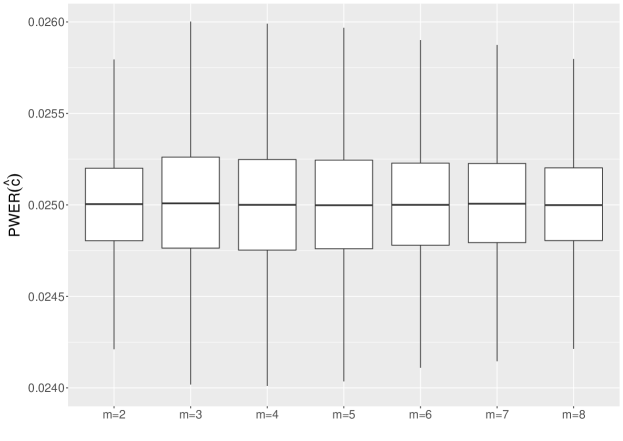
Figure 2: Distribution of $10^{4}$ simulated values of $\text{PWER}(\hat{c})$ for different numbers of biomarkers $m$. Outliers are omitted for better clarity. The significance level is $\alpha=0.025$ and the sample size is fixed at $N=500$.

$m$	Mean	SD	Min	Q1	Med	Q3	Max
2	0.02501	0.00032	0.02384	0.0248	0.025	0.0252	0.02635
3	0.02502	0.00038	0.02365	0.02476	0.02501	0.02526	0.02686
4	0.025	0.00039	0.02334	0.02475	0.025	0.02525	0.0266
5	0.025	0.00038	0.02341	0.02476	0.025	0.02524	0.02655
6	0.02501	0.00035	0.0233	0.02478	0.025	0.02523	0.02645
7	0.02501	0.00034	0.02357	0.02479	0.02501	0.02523	0.02667
8	0.02501	0.00032	0.02349	0.02481	0.025	0.0252	0.02667

Table 1: Summary statistics for the $10^{4}$ simulated values of $\text{PWER}(\hat{c})$ for $N=500$

Figure 3 shows 10 000 more simulated values of $\text{PWER}(\hat{c})$, whereby the number of biomarkers is now fixed at $m=3$ and the sample size varies. While larger inaccuracies can occur at sample sizes $N=25$ or $N=50$, for $N=100$ all values of the true PWER already deviate less than 15 percent from the significance level, and for $N=200$ less than 10 percent. So the mentioned convergence of $\text{PWER}(\hat{c})$ with respect to $N$ takes place very quickly and applies to practical situations.

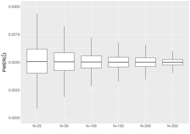
Figure 3: Distribution of $10^{4}$ simulated values of $\text{PWER}(\hat{c})$ for different sample sizes $N$. The number of biomarkers is fixed at $m=3$.

4.3 Constant prevalences

In figure 2, we see that the boxplot ranges also decrease as the number $m$ of populations increases. This is probably due to the fastly increasing number of strata and thus decreasing prevalences, so that single estimation inaccuracies in the strata-wise probabilities do not have a major impact on the PWER. In practice, of course, the sample size would have to be increased in order to have enough patients in all strata. We get similar results when we assume equal prevalences for all strata and leave them constant over all simulation runs. However, if individual prevalences remain constant with an increasing number of strata, this is not the case any more. This can be seen, for example, when one prevalence is set to 0.5 independently of the number of strata. The range of the simulated values then increases with increasing $m$, up to a standard deviation of $7.7\cdot 10^{-4}$ for $m=8$. The results for both of these cases can be found in the supplement to this paper.

4.4 Marginal sum estimator

Due to the independence of the biomarkers, another possibility of estimating the unknown prevalences is using the estimators

$$\tilde{\pi}_{J}=\left(\prod_{j\in J}\hat{\pi}_{j}\right)\left(\prod_{k\in I\setminus J}(1-\hat{\pi}_{k})\right),$$

which are based on the marginal frequencies $\hat{\pi}_{j}=\sum_{J\subseteq I:\,j\in J}\hat{\pi}_{J}$ of the $m$ overlapping populations. Under the indpendence assumption, this also gives consistent estimates. We obtain similar results when running the simulations like the ones in section 4.1. In this case, the deviation of the true PWER from $\alpha$ is slightly higher: The means are between 0.02501 (for $m=8$) and 0.02513 (for $m=2$) and the standard deviations are again between $3.2\cdot 10^{-4}$ and $3.9\cdot 10^{-4}$.

4.5 Correlated biomarkers and further cases

The assumption of independent biomarkers is not necessarily guaranteed in practice. But the above simulations can easily be extended to correlated biomarkers by deriving the biomarker probabilities from a normally distributed random vector with an arbitrary covariance matrix. We have done this for various cases and found no particular differences to the results of section 4.2. The same applies to the other cases treated in section 3, i.e. under the model with known variances (where the test statistics are normally distributed) and in the single treatment case, where we have $T_{i}=T$ for all $i\in I$ (with the simplified correlation matrix). The detailed results can be found in the supplement.

4.6 Behaviour of the maximal strata-wise FWER

In PWER-controlling test procedures, we are also interested in the behaviour of the single strata-wise family-wise error rates, which are defined by $\text{FWER}_{J}(c)\coloneqq\text{P}(\max_{j\in J}Z_{j}>c)$ for every $J\subseteq I$, to verify whether excessive type I error probabilities occur in individual strata. Brannath et al. (2023) give some upper bounds for $\text{FWER}_{J}(c)$, whose quality depend on different factors like the prevalence $\pi_{J}$ or the number of biomarkers the stratum $\mathcal{P}_{J}$ belongs to. Under the setup of the previous simulations, we also examined the actual values of the maximum $\max_{J\subseteq I}\text{FWER}(\hat{c})$. They are plotted in figure 4. We see that on average, they are all limited by $0.05=2\alpha$.

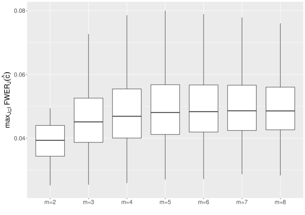
Figure 4: Distribution of $10^{4}$ simulated values of the maximal strata wise FWER for different numbers of biomarkers $m$. The sample size is fixed at $N=500$.

4.7 Introduction of a minimal prevalence for neglected strata

In the case of very small, but non-empty strata $\mathcal{P}_{J}$, it may happen that no patients are sampled from them, meaning that they are neglected by the estimated PWER. Then we would not directly account for the multiplicity in these strata and might therefore expose future patients to an increased risk of receiving inefficacious treatments. This is especially a problem when the strata are intersections of many different populations. If the biomarkers are independent, a solution could be to replace the MLE of $\pi$ with the marginal estimator $\tilde{\pi}$ from section 4.4. Since these estimates are based on the empirical marginal prevalences of the larger subpopulations $\mathcal{P}_{j}$, the problem of missed prevalences is avoided or at least much reduced. In the general case, one could introduce a minimal prevalence $\pi_{\text{min}}$ for all $\text{FWER}_{J}$ to be included in the estimated PWER, and reduce the other prevalences proportionally. It should not be chosen too large, as this could result in greater inaccuracy of the estimations (we replace the unbiased estimator $\hat{\pi}_{J}$ by an upwards biased value). One possible choice is $\pi_{\text{min}}=1/(2^{m+1}-2)$, i.e. half of the prevalence that each stratum would have if all strata were of same size. Given the very small value of $\pi_{\text{min}}$, especially for high numbers of biomarkers, we are then unlikely to overestimate the true prevalences. And this approach actually leads to more conservative tests: In additional simulations we restricted the biomarker probabilities $p_{1}$, …, $p_{m}$ to the interval $(0,0.2)$, in order to achieve that large intersections preferably get small prevalences. In a setting with $m=3$ populations, in $10^{4}$ simulation runs this resulted 4 229 times in at least one neglected strata. We then computed the critical boundary $\hat{c}$ and the adjusted $\hat{c}_{\text{min}}$ resulting from weighting up all neglected strata by $\pi_{\text{min}}$. Figure 5 compares the distributions of the true PWER and of the maximum FWER for these two boundaries. We see that for the unadjusted zero prevalences, the maximal FWER is increased in comparison to the previous simulation results, and is reduced to an acceptable level by the suggested adjustment of the prevalences. The true PWER is also becoming more conservative. For larger numbers of biomarkers $m$, this reduction becomes larger in absolute terms. For example, for $m=6$ the mean PWER decreases from 0.02501 to 0.01633 and the mean maximal FWER decreases from 0.1116 to 0.0740 by replacing $\hat{c}$ with $\hat{c}_{\text{min}}$. Note that $\hat{c}_{\text{min}}$ is not always larger than $\hat{c}$, especially when strata belonging to only few populations have small prevalences. Therefore we suggest comparing $\hat{c}$ and $\hat{c}_{\text{min}}$ and choosing the greater one for PWER control.

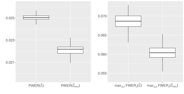
Figure 5: Comparison of the true PWER (left plot) and of the maximal strata-wise FWER (right plot) with and without the use of the minimal prevalence $\pi_{\text{min}}=1/(2^{m+1}-2)$, in a setting with $m=3$ popoulations, $N=500$ patients and $\alpha=0.025$

5 Discussion

We have seen that estimating the population prevalences in situations with up to eight different biomarkers and up to 255 strata does not prevent from adequate control of the true PWER. When interpreting the results from section 4, one should distinguish between individual values of the true PWER, which are conditioned to some vector $(n_{J})_{J\subseteq I}$ of sample sizes, and their mean over all simulation runs. An individual value of $\text{PWER}(\hat{c})$ is only meaningful for a specific study with a specific vector of sample sizes drawn from the multinomial distribution. We have seen a rather limited fluctation of these values. The unconditional PWER, where we average over all sample size configurations, approximates the expected PWER over many studies. For critical boundaries that are based on sample estimates of the prevalences, it is very well under control. In practice the situation may even be improved by also utilizing historical data in the estimation of the prevalences.

In section 3 we assumed that the variance of the observations is homogeneous between the different strata. In the inhomogeneous case, greater difficulties arise. The variances or their estimators then appear in the correlation matrix $\Sigma$, which makes its computation much more difficult, and thereby also PWER control. A general somewhat conservative solution is a Bonferroni based PWER control as described in Hsu et al. (to appear).

Another important prerequisite for the practical applicability of the PWER is the development of a sample size estimation for PWER-controlling studies, which is a topic for future research. The convergence of the rejection boundaries presented in appendix B could be of interest for this. Analogously to the PWER, a multiple power measure can be defined for studies with overlapping populations, the so-called population-wise power (PWP). It was introduced in Hillner (2021) and gives the average probability of correctly rejecting hypotheses that are relevant to the patients. Applying the approach from Section 4, we find that the PWP is also well controlled under the use of estimated prevalences.

Regarding the maximal strata-wise FWER, we have seen in the simulations that under PWER control it is often indirectly controlled at a higher level, here $2\alpha$. Note that there is no guarantee for this, so in practice the maximal FWER should always be taken into account in order to adjust the PWER or the prevalences used (if deemed necessary).

Appendix

A Proof of theorem 1

For $\theta\in\mathbb{R}^{m}$ and $J\subseteq I$ with $J\cap I_{0}(\theta)\neq\emptyset$ we have $\theta\in H_{J\cap I_{0}(\theta)}$. So according to the subset pivotality condition (1) there is a $\theta^{*}\in H_{I}$ with $\text{FWER}_{\theta}^{J}\coloneqq\text{P}_{\theta}\left(\max_{j\in J\cap I_{0}(\theta)}Z_{j}>c\right)=\text{P}_{\theta^{*}}\left(\max_{j\in J\cap I_{0}(\theta)}Z_{j}>c\right)\leq\text{P}_{\theta^{*}}\left(\max_{j\in J}Z_{j}>c\right).$ With the monotonicity (2) we get $\text{FWER}_{\theta}^{J}\leq\text{P}_{0_{\mathbb{R}^{m}}}\left(\max_{j\in J}Z_{j}>c\right)=\text{FWER}_{0_{\mathbb{R}^{m}}}^{J}.$ One concludes $\text{PWER}_{\theta}=\sum_{J\subseteq I}\pi_{J}\text{FWER}_{\theta}^{J}\leq\sum_{J\subseteq I}\pi_{J}\text{FWER}_{0_{\mathbb{R}^{m}}}^{J}=\text{PWER}_{0_{\mathbb{R}^{m}}}$.

B Convergence of the true PWER

Under the conditions of section 3.2 we assume that for every parameter $N\in\mathbb{N}$ of the multinomial distribution, and for each of its realizations $(n_{J})_{J\subseteq I}$, $\hat{c}_{N}$ is a critical value that satisfies $\widehat{\text{PWER}}(\hat{c}_{N})=\alpha$. The sequence $\left(\text{PWER}(\hat{c}_{N})\right)_{N\in\mathbb{N}}$ then almost surely converges to $\alpha$. This follows from $\text{PWER}(\hat{c}_{N})-\alpha=\text{PWER}(\hat{c}_{N})-\widehat{\text{PWER}}(\hat{c}_{N})=\sum_{J\subseteq I}\left(\pi_{J}-\hat{\pi}_{J}\right)\left(1-\Psi_{\nu_{J},\Sigma_{J}}\left(\hat{c}_{N},\dots,\hat{c}_{N}\right)\right)\xrightarrow[N\to\infty]{\text{a.s.}}0,$ in consequence of the strong consistency of the MLE $\hat{\pi}$ and the boundedness of $\Psi$.

The sequence $(\hat{c}_{N})_{N\in\mathbb{N}}$ of the estimated critical values is also convergent, in terms of convergence in probability, towards the critical limit $c(\pi)$ that results from using the true prevalences and correspondingly proportioned sample sizes. To prove this, we first note that for any fixed $c\in\mathbb{R}$ the estimated PWER $F_{N}(c)\coloneqq\widehat{\text{PWER}}_{\nu_{N},\Sigma_{N}}(c)$ converges in probability (and even almost surely) to $F(c)\coloneqq\text{PWER}_{\nu(\pi),\Sigma(\pi)}(c)$, where $\nu(\pi)$ and $\Sigma(\pi)$ are based on the true prevalences. This follows from the continuity of the multivariate t-distribution with respect to its location and scale matrix. Let $\varepsilon>0$ be given. Using the strong monotonicity of the PWER with respect to $c$, we find

$$\text{P}\left(\left|\hat{c}_{N}-c(\pi)\right|\geq\varepsilon\right) \leq\text{P}\left(\hat{c}_{N}\geq\varepsilon+c(\pi)\right)+\text{P}\left(\hat{c}_{N}\leq c(\pi)-\varepsilon\right)$$

$$\leq\text{P}\left(F_{N}\left(\varepsilon+c(\pi)\right)\geq\alpha\right)+\text{P}\left(F_{N}\left(c(\pi)-\varepsilon\right)\leq\alpha\right)$$

$$=\text{P}\left(F_{N}\left(\varepsilon+c(\pi)\right)-F(\varepsilon+c(\pi))\geq\alpha-F(\varepsilon+c(\pi))\right)$$

$$\quad+\text{P}\left(F(c(\pi)-\varepsilon)-F_{N}\left(c(\pi)-\varepsilon\right)\geq F(c(\pi)-\varepsilon)-\alpha\right),$$

and also some $\delta_{1},\delta_{2}>0$ with $F(\epsilon+c(\pi))=\alpha-\delta_{1}$ und $F(c(\pi)-\varepsilon)=\alpha+\delta_{2}.$ Hence with the pointwise convergence of $F_{N}$ to $F$ we get

$$\text{P}\left(\left|\hat{c}_{N}-c(\pi)\right|\geq\varepsilon\right) \leq\text{P}\left(\left|F_{N}\left(\varepsilon+c(\pi)\right)-F(\varepsilon+c(\pi))\right|\geq\delta_{1}\right)$$

$$\quad+\text{P}\left(\left|F(c(\pi)-\varepsilon)-F_{N}\left(c(\pi)-\varepsilon\right)\right|\geq\delta_{2}\right)\xrightarrow[N\to\infty]{}0+0=0.$$

Supplementary material

Supporting information for this article and the corresponding R program files are available under https://github.com/rluschei/PWER-Estimate-Prevalences.

References

- Brannath et al. (2023) Brannath, W., Hillner, C. and Rohmeyer, K. (2023). The population-wise error rate for clinical trials with overlapping populations. Statistical Methods in Medical Research. Vol. 32 (2) 334–352
- Hillner (2021) Hillner, C. (2021). Adaptive group sequential designs with control of the population-wise error rate. Universität Bremen, dissertation.
- Dickhaus (2014) Dickhaus, T. (2014). Simultaneous Statistical Inference. With Applications in the Life Sciences. Springer, Berlin, Heidelberg.
- Kshirsagar (1961) Kshirsagar, A. (1961). Some Extensions of the Multivariate t-Distribution and the Multivariate Generalization of the Distribution of the Regression Coefficient. Mathematical Proceedings of the Cambridge Philosophical Society Vol. 57 (1), 80-85.
- Westfall and Young (1993) Westfall, P. H. and Young, S. S. (1993). Resampling-based multiple testing. Examples and methods for p-value adjustment. Wiley series in probability and mathematical statistics, Applied probability and statistics. Wiley, New York.
- Hsu et al. (to appear) Hsu, J. C. et al. (to appear). Beyond conventional error rate control: decision-theoretic, conditional, Bayesian approaches: a panel discussion at MCP 2022.