Tetra-NeRF: Representing Neural Radiance Fields Using Tetrahedra

Abstract

Neural Radiance Fields (NeRFs) are a very recent and very popular approach for the problems of novel view synthesis and 3D reconstruction. A popular scene representation used by NeRFs is to combine a uniform, voxel-based subdivision of the scene with an MLP. Based on the observation that a (sparse) point cloud of the scene is often available, this paper proposes to use an adaptive representation based on tetrahedra obtained by Delaunay triangulation instead of uniform subdivision or point-based representations. We show that such a representation enables efficient training and leads to state-of-the-art results. Our approach elegantly combines concepts from 3D geometry processing, triangle-based rendering, and modern neural radiance fields. Compared to voxel-based representations, ours provides more detail around parts of the scene likely to be close to the surface. Compared to point-based representations, our approach achieves better performance. The source code is publicly available at: https://jkulhanek.com/tetra-nerf.

Figure 1: The input to Tetra-NeRF is a point cloud which is triangulated to get a set of tetrahedra used to represent the radiance field. Rays are sampled, and the field is queried. Barycentric interpolation is used to interpolate tetrahedra vertices, and the resulting features are passed through a shallow MLP to get the density and colours for volumetric rendering.

1 Introduction

Reconstructing 3D scenes from images and rendering photo-realistic novel views is a key problem in computer vision. Recently, NeRFs [39, 3, 4] became dominant in the field for their superior photo-realistic results. Originally, NeRFs used MLPs to represent the 3D scene as an implicit function. Given a set of posed images, NeRF randomly samples a batch of pixels, casts rays from the pixels into the 3D space, queries the implicit function at randomly sampled distances along the rays, and aggregates the sampled values using volumetric rendering [39, 37]. While the visual results of such methods are of high quality, the problem is that querying large MLPs at millions of points is costly. Also, once the network is trained, it is difficult to make any changes to the represented radiance field as everything is baked into the MLPs parameters, and any change has a non-local effect. Since then, there have been a lot of proposed alternatives to the large MLP field representation [41, 9, 17, 74, 70, 57, 32]. These methods combine an MLP with a voxel feature grid [41, 57], or in some cases represent the radiance field directly as a tensor [9, 10, 17]. When querying these representations, first, the containing voxel is found, and the features stored at the eight corner points of the voxel are trilinearly interpolated. The result is either passed through a shallow MLP [41, 57, 10, 9] or is used directly as the density and colour [17, 57, 32].

Having a dense tensor represent the entire scene is very inefficient, as we only need to represent a small space around surfaces. Therefore, different methods propose different ways of tackling the issue. Instant-NGP [41], for example, uses a hash grid instead of a dense tensor, where it relies on optimisation to resolve the hash collisions. However, similarly to MLPs, any change to the stored hashmap influences the field in many places. A more common direction to addressing the issue is by directly using a sparse tensor representation [17, 9]. These methods start with a low-resolution grid and, at predefined steps, subsample the representation, increasing the resolution. These approaches tend to require a careful setting of hyperparameters, such as the scene bounding box and the subdivision steps, in order for the methods to work well.

Because many of these methods use traditional structure from motion (SfM) [54, 55] methods to generate the initial poses for the captured images, we can reuse the original reconstruction in the scene representation. Inspired by classical surface reconstruction methods [22, 30, 29, 23], we represent the scene as a dense triangulation of the input point cloud, where the scene is a set of non-overlapping tetrahedra whose union is the convex hull of the original point cloud [14]. When querying such a representation, we find to which tetrahedron the query point belongs and perform barycentric linear interpolation of the features stored in the vertices of the tetrahedron. This very simple representation can be thought of as the direct extension of the classical triangle-rendering pipelines used in graphics [43, 45, 40]. The representation avoids problems with the sparsity of the input point cloud as the tetrahedra fully cover the scene, resulting in a continuous rather than discrete representation.

This paper makes the following contributions: (1) We propose a novel radiance field representation which is initialised from a sparse or dense point cloud. This representation is naturally denser in the proximity of surfaces and, therefore, provides a higher resolution in these regions. (2) The proposed representation is evaluated on multiple synthetic and real-world datasets and is compared with a state-of-the-art point-cloud-based representation – Point-NeRF [70]. The presented results show that our method clearly outperforms this baseline. We further demonstrate the effectiveness of our adaptive representation by comparing it with a voxel-based representation that uses the same number of trainable parameters. (3) We make the source code and model checkpoints publicly available.

2 Related work

Multi-view reconstruction.  The problem of multi-view reconstruction has been studied extensively and tackled with a variety of structure from motion (SfM) [61, 54, 63], and multi-view stereo (MVS) [55, 18, 12, 71] methods. These methods usually output the scene represented as a point cloud [54, 55]. In most rendering approaches, the point cloud is converted into a mesh [35, 24], and novel views are rendered by reprojecting observed images into each novel viewpoint and blending them together using either heuristically-defined [8, 13, 69] or learned [20, 50, 51, 73] blending weights.

However, the process of getting the meshes is usually quite noisy, and the resulting meshes tend to have inaccurate geometry in regions with fine details or complex materials. Instead of using noisy meshes, point-based neural rendering methods [26, 53, 38, 1] perform splatting of neural features and use 2D convolutions to render them. In contrast to these methods, our approach operates and aggregates features directly in 3D and does not suffer from the noise in the point cloud or the reconstructed mesh.

Neural radiance fields.  Recently, NeRFs [39, 77, 3, 4, 34] have gained a lot of attention thanks to their high-quality rendering performance. The original NeRF method [39] was extended to better handle aliasing artefacts in [3], to better represent unbounded scenes in [77, 4, 48], or to handle real-world captured images [36, 58]. The training of the large MLPs used in these methods can be quite slow, and there has been a lot of effort on speeding up either the training [41, 17, 9] or the rendering [48, 47, 74, 21] sometimes at the cost of larger storage requirements. Other approaches tackled different aspects of NeRFs like view-dependent artefacts [62], relighting [5, 7], or proposed generative models [64, 46]. Also, a popular research direction is making the models generalize across different scenes [11, 49, 28, 75, 66]. A large area of research is dedicated to the surface reconstruction and, instead of using the radiance fields, represents the scene implicitly by modelling the signed distance function (SDF) [76, 72, 65, 67, 52]. Unlike those approaches, we focus only on the radiance field representation and consider these methods orthogonal to ours.

Although there are some methods that train radiance fields while fine-tuning the poses [31, 60] or without known cameras [68, 6], most methods need camera poses for the reconstruction. SfM, e.g., COLMAP [54, 55], is typically used for estimating the poses, which also produces a (sparse) point cloud. Our approach makes use of this by-product of the pose recovery process instead of only using the poses themselves.

Field representations.  When a single MLP is used to represent the entire scene, everything is baked into a single set of parameters which cannot be easily modified, because any change to the parameters has a non-local effect, i.e., it changes the scene at multiple unrelated places. To overcome this problem, others have experimented with different representations of the radiance fields [17, 57, 41, 9, 70, 32, 10, 44]. A common practice is to represent the scene as a shallow MLP and an efficiently encoded voxel grid [32, 41, 9, 10, 44]. The encoded voxel grid can also be used represent the radiance field directly [17, 57]. The voxel grid can be encoded as a sparse tensor [57, 17, 32], a factorisation of the 4D tensor [9, 10], or a hashmap [41]. When these structures are queried, trilinear interpolation is used to combine the feature vectors stored in the containing voxel corners. Unfortunately, the hashmaps [41] and hierarchical representations [10] have the same non-local effect problem, and the rest of the approaches rely on subsequent upsampling of the field and can be overly complicated. Also, feature vectors cannot be placed arbitrarily in the 3D space as they must lie on the grid with a fixed resolution. In contrast, our approach is much more flexible as it stores the feature vectors freely in 3D space.

Finally, Point-NeRF [70] represents the scene as a point cloud of features which are queried using $k$-nearest neighbours search. However, when the point cloud contains sparse regions, the rays do not intersect any neighbourhoods of any points and the pixels stay empty without the ability to optimise. Therefore, Point-NeRF [70] relies on gradually adding more points during training and increasing the scene complexity. Since we use the triangulation of the point cloud rather than the discrete point cloud itself, our representation is continuous and does not suffer from empty regions. Therefore, we do not have to add any points during training.

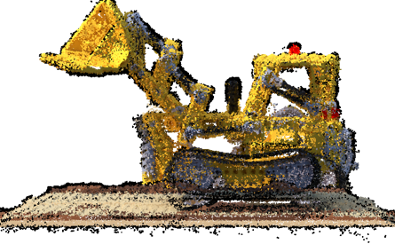
(a) dense point cloud

(b) dense tetrahedra slice

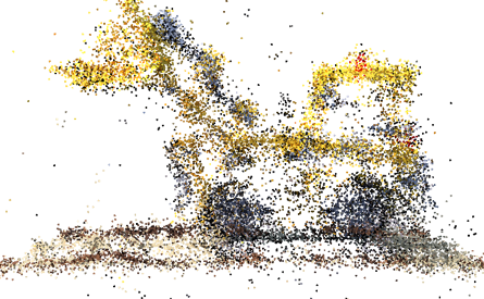
(c) sparse point cloud

(d) sparse tetrahedra slice

Figure 2: Input point cloud and a slice through the triangulated tetrahedra. Note that smaller tetrahedra are created closer to the surface of the scene, i.e., regions close to the surface are represented with a finer resolution.

3 Method

A common strategy in the literature is to represent the scene explicitly through a voxel volume. In contrast to this uniform subdivision, we investigate using an adaptive subdivision of the scene. In many scenarios, an approximation of the scene geometry is either given, e.g., when using SfM to compute the input camera poses, or can be computed, e.g., via MVS or single-view depth predictions [79]. This allows us to compute an adaptive subdivision of the scene via Delaunay triangulation [14] of such a point cloud. This results in a set of non-overlapping tetrahedra, where smaller tetrahedra are created close to the surface of the scene (c.f. Fig. 2). In the following, we explain how this adaptive subdivision of the scene can be used instead of voxels for volume rendering and neural rendering.

(a) trilinear interpolation

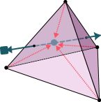
(b) barycentric interpolation

Figure 3: Trilinear and barycentric intepolation. Trilinear interpolation is a weighted combination of the eight voxel corners. Barycentric interpolation weights the four vertices of the tetrahedron vertices based on the barycentric coordinates [16].

3.1 Preliminaries

Neural Radiance Fields (NeRFs) [39] represent a scene through an implicit function $F(\mathbf{x},\mathbf{d})$, often modelled via a neural network, that returns a colour value and a volume density prediction for a given 3D point $\mathbf{x}$ in the scene observed from a viewing direction $\mathbf{d}$. Volume rendering [37] is used to synthesise novel views: for each pixel in a virtual view, we project a ray from the camera plane into the scene and sample the radiance field to obtain the colour and density values $\mathbf{c}_{i}$ and $\sigma_{i}$ at distances $t_{i}$ along the ray, where $i=1\ldots N$. The individual samples are then combined to predict the colour $\mathbf{C}$ for the pixel:

$$\begin{split}\mathbf{C}&=\sum_{i=1}^{N}T_{i}(1-\exp(\sigma_{i}\delta_{i}))\mathbf{c}_{i}\enspace,\text{where}\\ T_{i}&=\exp(-\sum_{i=1}^{N-1}\sigma_{i}\delta_{i})\enspace,\end{split}$$ (1)

and $\delta_{i}=t_{i}-t_{i-1}$ is the distance between adjacent samples. This process is fully differentiable. Thus, after computing the mean squared error (MSE) between the predicted and ground truth colours associated with each ray, we can back-propagate the gradients to the radiance field.

Voxel-based feature fields such as NSVF [32] represent the scene as a voxel grid and an MLP. Each grid point of the voxel grid is assigned a trainable vector. There are eight feature vectors associated with a single voxel, but the vectors are shared between neighbouring voxels. For each query point sampled along the ray, its corresponding voxel is found first. A feature for the point is then computed via trilinear interpolation of the features of the voxel grid points based on the position of the query point (c.f. Fig. 3, left). The resulting feature vector is passed through an MLP to predict the density and appearance vector. The appearance vector is combined with the ray direction and passed through a second MLP in order to compute a view-dependent colour.

3.2 Tetrahedra fields

Given a set of points in 3D space, we build the tetrahedra structure by triangulating the points. We apply the Delaunay triangulation [14] to obtain a set of non-overlapping tetrahedra whose union is the convex hull of the original points. Fig. 2 shows example tetrahedra obtained by triangulating dense and sparse COLMAP-reconstructed point clouds [54, 55]. Note that the resulting representation is adaptive as it uses a higher resolution (smaller tetrahedra) closer to the surface and larger tetrahedra to model regions farther away from the surface.

We associate all vertices of the tetrahedra with trainable vectors. As in the voxel grid case, vertices, and thus vectors, are shared between adjacent tetrahedra. The resulting tetrahedra field can be queried in the same way a voxel grid representation is queried: for each query point, we first find the tetrahedron containing the point. Instead of the trilinear interpolation used for voxel volumes, we use the barycentric interpolation [16] to compute a feature vector for the query point from the four feature vectors stored at the tetrahedron’s vertices (c.f. Fig. 3). To this end, we compute the query point $\mathbf{x}$’s barycentric coordinates $\bm{\lambda}$, which express the point’s 3D coordinates as a unique weighted combination of the 3D coordinates of the tetrahedron’s vertices. In particular, the weight for a vertex is the volume of the tetrahedron constructed from the query point and the face opposite to the vertex divided by the volume of the full tetrahedron:

$$\bm{\lambda}=\bigg{(}\frac{V_{x234}}{V_{1234}},\frac{V_{1x34}}{V_{1234}},\frac{V_{12x4}}{V_{1234}},\frac{V_{123x}}{V_{1234}}\bigg{)}\,,$$ (2)

where $V_{1234}$ is the volume of the full tetrahedron and $V_{x234}$, $V_{1x34}$, …, are volumes of tetrahedra with $1^{\text{st}}$, $2^{\text{nd}}$, …, vertex replaced by $\mathbf{x}$. The same weights $\bm{\lambda}$ are applied to the feature vectors of the vertices to obtain the query feature.

The interpolated features are used as the input to a small MLP in order to predict density and colour at the query point. We first pass the barycentric-interpolated features through a three-layer MLP to compute the density and appearance features. We then concatenate the appearance features with the ray direction vector encoded using Fourier features [59, 39] and pass the result through a single linear layer to get the raw RGB colour value.

Finally, to map the raw density values $\bar{\sigma_{i}}$ returned by the network to the volume density $\sigma_{i}$ required by volume rendering, we apply the softplus activation function [3]. For the RGB colour value, we use the sigmoid function [17].

3.3 Efficiently querying a tetrahedra field

Determining the corresponding voxel for a given query point can be done highly efficiently via hashing [42]. In contrast, finding the corresponding tetrahedron for a query point is more complex. This in turn can significantly impact rendering, and thus training, efficiency [17, 41, 57].

In order to efficiently look up the corresponding tetrahedra, we exploit that we are not considering isolated points, but points sampled from a ray. We compute the tetrahedra that are intersected by the ray, allowing us to march through the tetrahedra rather than computing them individually per point. The relevant tetrahedra can be found efficiently using acceleration structures for fast ray-triangle intersection computations, e.g., via NVidia’s OptiX library [43]: We first compute the intersections between the rays from a synthetic view and all faces of the tetrahedra. For each ray, we take the first 512 intersected triangles, and determine the corresponding tetrahedra. The tetrahedra can be ordered based on the intersections along the ray, allowing us to easily march through the tetrahedra to determine which tetrahedron to use for a given query point.

A side benefit of computing ray-triangle intersections is that we can simplify computing the barycentric coordinates: For each intersection, we compute the 2D barycentric coordinates w.r.t. the triangle. We then obtain the 3D barycentric coordinates w.r.t. the associate tetrahedron by simply adding zero for the vertex opposite to the triangle. For a query point inside a tetrahedron, we can compute its tetrahedron barycentric coordinates by linearly interpolating between the barycentric coordinates of the two intersections of the ray and the tetrahedron.

3.4 Coarse and fine sampling

We follow the common practice of having a two-stage sampling procedure [39, 9]. In the coarse stage, we sample uniformly along the ray. In the fine stage, we use the density weights from the coarse sampling stage to bias the sampling towards sampling closer to the potential surface. Following [39], we use the stratified uniform sampling for the coarse stage. The stratified uniform sampling splits the ray into equally long intervals and samples uniformly in each interval. Unlike NeRF [39], we limit the sampling to the space occupied by tetrahedra. In the fine sampling stage, we use the same network as in the coarse sampling stage.

For the fine sampling stage, we take the accumulated weights $w_{i}$ from the coarse sampling:

$$\bar{w_{i}}=(1-\exp(-\sigma_{i}\delta_{i}))\exp\bigg{(}-\sum_{j=1}^{i-1}\sigma_{j}\delta_{j}\bigg{)}\enspace.$$ (3)

These weights are the coefficients used in Equation 1 as multipliers for the colours [39]. We obtain $w_{i}$ by normalizing $\bar{w_{i}}$. Following [39], we sample set of fine samples using weight $w_{i}$. To render the final colour, we merge the dense and fine samples and use all in the rendering equation [9].

4 Experiments

We compare Tetra-NeRF to relevant methods on the commonly used synthetic Blender [39], the real-world Tanks and Temples [25], and the challenging object-centric Mip-NeRF 360 [4] datasets. To show its effectiveness, we compare Tetra-NeRF to a dense-grid representation and evaluate it with reduced quality of the input point cloud. We start by describing the exact hyperparameters used.

4.1 Implementation details

Generating point cloud & triangulation. Given a set of posed images, we use the COLMAP reconstruction pipeline [54, 55] to get the point cloud used in our tetrahedra field representation. We then reduce the size of the resulting point cloud such that if the number of points is larger than $10^{6}$, we subsample $10^{6}$ points randomly. For the Blender dataset experiments, where the number of points is smaller, we add more randomly generated points. In that case, the number of random points is half the number of original points. The reason for adding the points is that with a low number of points, some pixels on edges may not intersect any tetrahedra, potentially producing artefacts on the edges. Each added point is sampled as follows: we sample a random point $x_{0}$ from the original point cloud, sample a random normal vector $n$, and a number $\alpha\sim\mathcal{N}(\bar{d},\,\bar{d}^{2})$, where $\bar{d}$ is the average spacing of the original point cloud, i.e. the average distance between each point and its six closest neighbours. We then add the point $x=x_{0}+\alpha n$.

Initialization. Given the processed point cloud, we apply the Delaunay triangulation [14] to get a set of tetrahedra. To this end, we use the CGAL library [2], which in our experiments runs in the order of milliseconds. Following [41], we initialise the features of size $64$ at the vertices of the tetrahedra with small values sampled uniformly in the range $-10^{-4}$ to $10^{-4}$. However, to allow the model to reuse the information contained in the point cloud, we set the first four dimensions of the feature field to the RGBA colour values (rescaled to interval $[0,1]$) stored at the associated points in the point cloud. The alpha value of all original points is one, whereas all randomly sampled points have an alpha value of zero. For the MLP, we follow the common practice of using the Kaiming uniform initialisation [19]. The hidden sizes in all MLPs are 128.

Training. During training, we sample batches of 4,096 random rays from random training images. We use volumetric rendering to predict the colour of each ray. The gradients are computed by backpropagating the MSE loss between the predicted colour and the ground truth colour value. We use the RAdam optimizer [33] and decay the learning rate exponentially from $10^{-3}$ to $10^{-4}$ in $300$k steps. The training code is built on top of the Nerfstudio framework [60], and the tetrahedra field is implemented in CUDA and uses the OptiX library [43]. We train on a single NVIDIA A100 GPU and the training speed ranges from 15k rays per second to 30k rays per second. The speed depends on how well-structured the triangulation is, how many vertices there are, and if there is empty space around the object. The full training with 300k iterations takes between $11$ and $24$ hours, depending on the scene complexity. However, good results are typically obtained much earlier, e.g., in 100k iterations.

4.2 Results

Blender dataset [39] results. 

	PSNR $\uparrow$	SSIM $\uparrow$	LPIPS $\downarrow$
NeRF[39]	31.00	0.947	0.081
NSVF[32]	31.77	0.953	-
mip-NeRF[3]	tab_red 34.51	0.961	orange 0.043
instant-NGP[41]	yellow 33.18	-	-
Plenoxels[17]	31.71	0.958	yellow 0.049
Point-NeRFcol[70]	31.77	yellow 0.973	0.062
Point-NeRFmvs[70]	orange 33.31	orange 0.978	yellow 0.049
Tetra-NeRF	32.53	tab_red 0.982	tab_red 0.041

Table 1: Results on the Blender dataset [39] averaged over all scenes in the dataset. Even though we use the same input point cloud as Point-NeRF^col, we outperform it greatly. We perform on par with Point-NeRF^mvs even though it uses many more points and densifies the point cloud during training. We highlight the best, second, and third values.

Figure 4: Qualitative results on the Blender dataset. We compare with Point-NeRF^col as we use the same input point cloud. In the top-row picture, we can see that Tetra-NeRF is able to represent fine details well on the mic scene. On the drums scene (2${}^{\text{nd}}$ row), both methods struggle with shiny materials, but our method performs slightly better. 3${}^{\text{rd}}$ row: Tetra-NeRF can render thin ropes. Bottom row: accumulation is nonzero in areas close to surface.

We compare to relevant baselines on the standard Blender dataset. We used the same split and evaluation procedure as in the original NeRF paper [39] and the same SSIM implementation as Point-NeRF [70]. In order to ensure a fair comparison with Point-NeRF [70] when COLMAP points were used, we use the exact same COLMAP reconstruction as Point-NeRF. We report the PSNR, SSIM, and LPIPS (VGG) [78] metrics. Tab. 1 shows averaged results, Fig. 4 shows qualitative results, and the results for individual scenes are given in Supp. Mat.

When we use the exact same COLMAP points as Point-NeRF (row Point-NeRF^col), we outperform it in all three metrics. We score comparably with Point-NeRF^mvs, even though it starts from a much denser and higher-quality initial point cloud, which it generates from a jointly trained model. Also note that both of these Point-NeRF configurations grow the point cloud during training and, therefore, the complexity of the scene representation grows. For us, the points are fixed, and the number of parameters stays the same. We also outperform Plenoxels [17], which uses a sparse grid. Note that same as Point-NeRF, Plenoxels also gradually increases the representation complexity by subdividing the grid resolution at predefined training epochs. Even though both Mip-NeRF and instant-NGP outperform our approach in terms of PSNR, our method is slightly better in terms of SSIM, and on par with Mip-NeRF in terms of LPIPS.

	hotdog		ship
	PSNR $\uparrow$	SSIM $\uparrow$	PSNR $\uparrow$	SSIM $\uparrow$
Point-NeRFstatic	29.91	0.978	19.35	0.905
Tetra-NeRF	33.31	0.989	31.13	0.994

Table 2: Comparison with Point-NeRF with disabled point cloud growing and prunning shows that Point-NeRF performs significantly worse in all measured metrics because it struggles to handle the sparse point clouds.

To analyze the tetrahedra field representation, we compare it with the point cloud field representation used in Point-NeRF. In Table 2, we compare our method to Point-NeRF when we disable point cloud growth and pruning. We show the results on two scenes from the Blender dataset [39] which were selected in the Point-NeRF paper. With this setup, we vastly outperform Point-NeRF in all metrics. The reason is that Point-NeRF requires the point cloud to be dense such that all rays have a chance to intersect a neighbourhood of a point. Since we use a continuous representation (tetrahedra field) rather than a discrete one, we can achieve good results even for sparser point clouds.

Comparison with the dense grid representation. 

Figure 5: Comparison with dense grid field representation. Tetra-NeRF on the left, dense grid on the right. We used a comparable number of parameters for both methods (the dense grid having slightly more parameters). Due to the adaptive nature of tetrahedra fields, Tetra-NeRF produces significantly better rendering as it is able to focus on relevant parts of the scene.

In order to show the utility of the adaptive tetrahedra field representation, we compare it to a dense grid representation. Similarly to NSVF [32], we split the 3D scene bounding box into equally-sized voxels. When querying the field, we find the voxel to which the query point belongs and perform trilinear interpolation of the eight corners of the voxel. We choose the grid resolution such that the number of grid points is the lowest cube number larger than the number of points of the original point cloud. This ensures a fair comparison as the baseline uses a comparable (but larger) number of features than our approach. All other hyperparameters are kept the same as for Tetra-NeRF. We evaluate both approaches on two scenes from the Blender dataset [39]. The dense grid representation only scores PSNR $18.81$ and $18.91$ on the lego and ship scenes, respectively, whereas Tetra-NeRF scores PSNR $33.79$ and $30.69$, respectively. The results can be seen in Figure 5. Note that in this experiment, we only trained for $100,000$ iterations to save computation time. From the numbers and the figure, we can clearly see that the dense grid resolution is not sufficient to reconstruct the scene in enough detail. Because Tetra-NeRF uses an adaptive subdivision, which is more detailed around the surface, we are better able to focus on relevant scene parts. With a similar number of trainable parameters, we thus obtain better results.

Tanks and Temples [25] dataset. 

	PSNR $\uparrow$	SSIM $\uparrow$	LPIPS $\downarrow$
NV [34]	23.70	0.848	0.260
NeRF [39]	25.78	0.864	0.198
NSVF [32]	orange 28.40	yellow 0.900	yellow 0.153
Point-NeRF [70]∗	yellow 28.35	orange 0.942	orange 0.090
Tetra-NeRF	tab_red 28.90	tab_red 0.957	tab_red 0.059

Table 3: Result on the Tanks and Temples dataset [25] as processed by NSVF [32] averaged over all scenes. We show the PSNR, SSIM, and LPIPS (Alex) [78] metrics. We highlight the best, second, and third values. ^∗Note, that Point-NeRF [70] results differ from the paper as they were recomputed with the resolution used in other methods.

Figure 6: Results on Tanks and Temples dataset. In the top row, we can see that we are able to represent the rim of the wheel better than Point-NeRF. Similarly, we can represent the tyre better in the third row. Finally, in the bottom, Point-NeRF fails on the wall and the roof, whereas Tetra-NeRF can render these parts well.

To be able to compare with Point-NeRF [70] on real-world data, we have evaluated Tetra-NeRF on the Tanks and Temples [25] dataset. We use the same setup as in NSVF [32], where the object is masked. We report the usual metrics: PSNR, SSIM, and LPIPS (Alex). We used the dense COLMAP reconstruction to get the point cloud used in the tetrahedra field. Quantitative results are shown in Table 3, qualitative results are presented in Figure 6, and the per-scene results are given in the Supp. Mat. Note that the results originally reported in the Point-NeRF paper [70] were evaluated with a resolution different from the compared methods. Therefore, to ensure a fair comparison, we have recomputed the metrics in the publicly available Point-NeRF’s predictions with the full resolution of $1920\times 1080$ as used in NSVF [32]. In the public dataset, one of the scenes had corrupted camera parameters and we had to reconstruct the poses again for the Ignatius scene. With the reconstructed poses, our method performs slightly worse on that scene compared to others.

The results show that our method outperforms the baselines in all compared metrics. This indicates that even though Point-NeRF relies on the ability to grow the point cloud density during training, this is not needed when using a continuous instead of a discrete representation.

	Outdoor			Indoor			Mean
	PSNR $\uparrow$	SSIM $\uparrow$	LPIPS $\downarrow$	PSNR $\uparrow$	SSIM $\uparrow$	LPIPS $\downarrow$	PSNR $\uparrow$	SSIM $\uparrow$	LPIPS $\downarrow$
NeRF [39, 15]	21.46	0.458	0.515	26.84	0.790	0.370	23.85	0.605	0.451
mip-NeRF [3]	21.69	0.471	0.505	26.98	0.798	0.361	24.04	0.616	0.441
NeRF++ [77]	22.76	0.548	0.427	28.05	0.836	0.309	25.11	0.676	0.375
Deep Blending [20]	21.54	0.524	0.364	26.39	0.844	0.261	23.70	0.666	0.318
Point-Based Neural Rendering [26]	21.66	yellow 0.612	0.302	26.28	yellow 0.887	0.191	23.71	yellow 0.734	yellow 0.253
Stable View Synthesis [51]	yellow 23.01	orange 0.662	tab_red 0.253	yellow 28.22	orange 0.907	orange 0.160	yellow 25.33	orange 0.771	tab_red 0.211
mip-NeRF 360 [4]	tab_red 23.72	tab_red 0.687	orange 0.282	orange 29.43	tab_red 0.911	yellow 0.181	orange 26.26	tab_red 0.786	orange 0.237
Tetra-NeRF	orange 23.17	0.586	yellow 0.298	tab_red 30.21	0.881	tab_red 0.103	tab_red 26.30	0.717	tab_red 0.211

Table 4: Mip-NeRF 360 dataset results. We show the PSNR, SSIM, and LPIPS (Alex) [78] on two categories of Mip-NeRF 360 [4] scenes: outdoor, and indoor. On the outdoor scenes, we outperform the Stable View Synthesis [51] and are comparable to Mip-NeRF 360 [4], even though our method does not implement the improvements suggested in NeRF++ [77] and Mip-NeRF 360 [4], and is more comparable to vanilla NeRF [39]. We highlight the best, second, and third values.

Sparse and dense point cloud comparison. 

(a) sparse point cloud

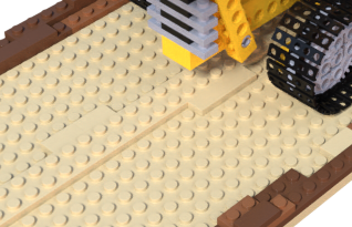
(b) ground-truth image

(c) sparse model

(d) dense model

Figure 7: Sparse vs. dense model comparison detail. Even though the area in the bottom contains few points, we are still able to reconstruct at least low-frequency data.

	sparse		dense
	PSNR/SSIM	#points	PSNR/SSIM	#points
Blender/lego	29.77/0.959	25,784	33.79/0.985	302,781
Blender/ship	26.90/0.899	7,152	30.69/0.942	321,861
360/bonsai	28.12/0.902	413,226	28.34/0.902	1,000,000
360/garden	24.79/0.806	227,532	25.41/0.838	1,000,000

Table 5: Dense and sparse point cloud comparison. We present results on two scenes from the Blender [39] and Mip-NeRF 360 [4] datasets. We also show the number of vertices of the tetrahedra field – including the randomly sampled points.

Previous experiments have used dense COLMAP reconstructions. However, dense point clouds may not be required to achieve good reconstructions. In this section, we compare models trained on dense reconstructions and sparse reconstructions. Table 5 compares PSNR, and SSIM metrics on two synthetic scenes from the Blender dataset [39] and two real-world scenes from the Mip-NeRF 360 dataset [4]. We also show the number of vertices of the tetrahedra, which is the size of the input point cloud, including the random points added at the beginning. Note that in this experiment, we only trained for $100,000$ iterations to save computation time.

From the results, we can see that for the Blender dataset [39] case, the dense model is much better. This is to be expected since the number of points obtained from the sparse reconstruction on the Blender dataset is very small and our MLP does not have enough capacity to represent fine details. However, even in regions with zero point coverage, we are still able to provide at least some low-frequency data (c.f. Fig. 7). On real-world scenes, the sparse point cloud model is almost on par with the dense one. The sparse reconstructions on the real-world dataset provide many more points compared to the synthetic dataset case, and the coverage is sufficient. From these results, we conclude that on real-world data the sparse model can be sufficient to achieve good performance.

Mip-NeRF 360[4] dataset. 

Figure 8: Mip-NeRF 360 results. 1${}^{\text{st}}$ row: we show the results on the garden scene. 2${}^{\text{nd}}$: we can see that Tetra-NeRF has some problems rendering grass. 3${}^{\text{rd}}$: Tetra-NeRF is able to represent the delicate texture of the tablecloth well. 4${}^{\text{th}}$: Tetra-NeRF is able to recover fine geometry.

We have further evaluated our method on the Mip-NeRF 360 [4] dataset. In order to ensure a fair comparison with Mip-NeRF 360 [4], we trained and evaluated on four times downsized images for the outdoor scenes and two times downsized images for the indoor scenes. The quantitative results are presented in Table 4, and the qualitative results are shown in Figure 8.

From the results, we can see that Tetra-NeRF is able to outperform both the vanilla NeRF [39] and Mip-NeRF [3]. We also outperform Stable View Synthesis [51] in terms of PSNR and score comparably in terms of LPIPS. This is possible because outdoor scenes contain a lot of high-resolution geometries, such as leaves and Stable View Synthesis is not able to overcome noise in the approximate geometry. Tetra-NeRF does not suffer from these problems as we aggregate features in 3D along rays rather than on the surface. Mip-NeRF 360 scores comparably to Tetra-NeRF in terms of PSNR and LPIPS, but it outperforms Tetra-NeRF in terms of SSIM. However, Mip-NeRF 360 implements some tricks designed to boost its performance. On the other hand, our approach is based on vanilla NeRF, and we believe that the performance can be boosted similarly.

Varying the number of input points  We conducted a study on the effect of the input point cloud size on the reconstruction quality. We consider both the sparse and the dense point clouds and analyse the performance as we sub-sample the points or add more points randomly. We evaluate on the family and the truck scenes from the Tanks and Temples [25] (tt) dataset, and the room and the garden scenes from the Mip-NeRF 360 [4] dataset. The sizes of sparse point clouds were roughly 16K, 30K, 113K, and 139K respectively and the sizes of dense point clouds were larger than 5M for all scenes. When the size of the original point cloud was larger than the desired size, we selected points uniformly at random, and when smaller, we added new random points as described Section 4.1. We include detailed results in the Supp. Mat. In order to save computational resources, we only train the method for $100$k iterations. The results are visualised in Figure 16.

As expected, the performance improves with the number of points used, as it leads to a finer subdivision of the scene around the surface. We can also observe (e.g., from tt/family) that the sparse reconstruction leads to a better reconstruction quality at the same point cloud size. The likely explanation is that sampling uniformly at random will be biased towards regions with high density and some regions may be missed or covered extremely sparsely.

Speed of convergence 

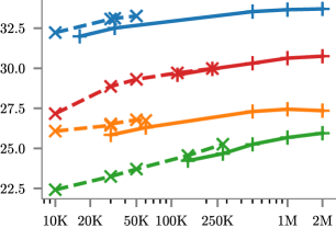
(a) Different point cloud sizes (PSNR)

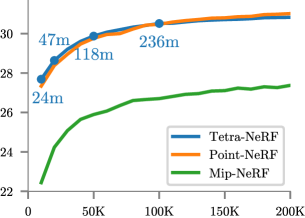
(b) Training performance on blender/ship (PSNR)

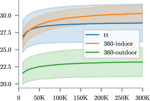
(c) Training performance (PSNR)

Figure 9: a) shows the PSNR with different sizes of input point clouds. The solid and dashed lines represent the dense and coarse COLMAP reconstructions. The following scenes were evaluated (best to worst): tt/family, 360/room, tt/truck, and 360/garden from Tanks and Temples [25] (tt) and Mip-NeRF 360  [4] (360-indoor/360-outdoor) datasets. As expected, the quality increases with the number of points. b) visualizes the training speed (PSNR at different training iterations) on the blender/ship scene [39]. It shows Tetra-NeRF training times for various timesteps and compares the rate of convergence with Point-NeRF [70] and Mip-NeRF [3]. Similarly, c) shows the rate of convergence aggregated over Tanks and Temples [25] (tt) and Mip-NeRF 360  [4] (360-indoor/360-outdoor) datasets. It shows the average PSNR, and the highlighted area represents the standard deviation.

Figures 8b, 8c show the rate of convergence on the ship scene from the Blender dataset and aggregated results on the Tanks and Temples [25], and Mip-NeRF 360 (indoor/outdoor) [4] datasets. Similar to PointNeRF, good results can be achieved quite early in the training process. E.g., on the blender/ship scene, in 24 minutes, our method achieves performance similar to Mip-NeRF [3] after several hours of training. The efficiency of the implementation is a large factor in the speed of different methods. E.g., in Instant-NGP [41], the authors invested a significant effort in optimizing GPU memory accesses, and the result is highly optimised efficient code (a main contribution of [41]). There are several places where our implementation can easily be made more efficient. E.g., changing the memory layout (row-major vs. column-major) of the tetrahedra field leads to a 10% speedup.

5 Limitations

(a) Failure case 1: low point cloud density on the ground

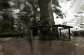
(b) Failure case 2: too many intersected tetrahedra

Figure 10: Failure cases. Left: barn scene from [25]. Right: tree hill scene from [4].

One drawback of our approach is that the quality of different regions of the rendered scene depends on the density of the point cloud in these regions. If the original point cloud was constructed using 2D feature matching, there can be regions with a very low number of 3D points. We show such an example in Fig. 9a. There are few 3D points on the ground, resulting in blurry renderings for that region.

Another issue is that the current implementation has a limit on the number of intersected tetrahedra per ray. For large or badly structured scenes, where rays intersect many tetrahedra, this can limit the reconstruction quality. Fig. 9b shows such a case on a Mip-NeRF 360 scene [4]. This problem can be addressed by increasing the limit on the number of visited tetrahedra at the cost of higher memory requirements and run-time. Alternatively, coarse-to-fine schemes that start with a coarser tetrahedralisation and prune the space could potentially handle this issue.

6 Conclusion

This paper proposes a novel radiance field representation that, compared to standard voxel-based representations, is easily able to adapt to 3D geometry priors given in the form of a (sparse) point cloud. Our approach elegantly combines concepts from geometry processing (Delaunay triangulation) and triangle-based rendering (ray-triangle intersections) with modern neural rendering approaches. The representation has a naturally higher resolution in the space near surfaces, and the input point cloud provides a straightforward way to initialise the radiance field. Compared to Point-NeRF, a state-of-the-art point cloud-based radiance field representation which uses the same input as our approach, Tetra-NeRF shows clearly better results. Our method performs comparably to state-of-the-art MLP-based methods. The results demonstrate that Tetra-NeRF is an interesting alternative to existing radiance field representations that is worth further investigation. Interesting research directions include adaptive refinement and pruning of the tetrahedralisation and exploiting the fact that the surface of the scene is likely close to some of the triangles in the scene.

Acknowledgements  This work was supported by the Czech Science Foundation (GAČR) EXPRO (grant no. 23-07973X), the Grant Agency of the Czech Technical University in Prague (grant no. SGS22/112/OHK3/2T/13), and by the Ministry of Education, Youth and Sports of the Czech Republic through the e-INFRA CZ (ID:90254).

Supplementary Material

First, in Section A, we describe the attached video where we illustrate the tetrahedra field and the optimisation process. Next, we extend Sections 4.2, 4.3, and 4.4 from the main paper by giving detailed results on the Blender [39], Tanks and Temples [25], and Mip-NeRF 360 [4] datasets in Sections B, C, and D. Finally, we extend Section 4.5 from the main paper and evaluate how the performance changes when varying the size of the input point cloud in Section E.

Appendix A Attached video

To present the idea of the paper visually, we include a video illustrating the tetrahedra field representation and showing the results of the optimisation at different points in the early stages of the training. In the video, we used the garden scene from the Mip-NeRF 360 dataset [4]. We show the optimisation using both the sparse and the dense input point clouds. The video starts by showing the initial point cloud and the tetrahedra obtained by the Delaunay triangulation. It then shows how the scene is optimised from the first iteration. Finally, it presents the resulting video generated by the fully trained model.

Appendix B Blender results

	PSNR$\uparrow$
	chair	drums	ficus	hotdog	lego	materials	mic	ship	mean
NPBG [1]	26.47	21.53	24.60	29.01	24.84	21.58	26.62	21.83	24.56
NeRF [39]	33.00	25.01	30.13	36.18	32.54	29.62	32.91	28.65	31.01
NSVF [32]	33.19	25.18	31.23	37.14	32.54	tab_red 32.68	34.27	27.93	31.77
Mip-NeRF [3]	tab_red 37.14	tab_red 27.02	33.19	tab_red 39.31	orange 35.74	orange 32.56	tab_red 38.04	tab_red 33.08	tab_red 34.51
Instant-NGP [41]	35.00	yellow 26.02	orange 33.51	orange 37.40	tab_red 36.39	yellow 29.78	orange 36.22	yellow 31.10	yellow 33.18
Plenoxels [17]	33.98	25.35	31.83	36.43	34.10	29.14	33.26	29.62	31.71
Point-NeRFcol [70]	yellow 35.09	25.01	33.24	35.49	32.65	26.97	35.54	30.18	31.77
Point-NeRFmvs [70]	orange 35.40	orange 26.06	tab_red 36.13	yellow 37.30	yellow 35.04	29.61	yellow 35.95	30.97	orange 33.31
Tetra-NeRF	35.05	25.01	yellow 33.31	36.16	34.75	29.30	35.49	orange 31.13	32.53
	SSIM$\uparrow$
	chair	drums	ficus	hotdog	lego	materials	mic	ship	mean
NPBG [1]	0.939	0.904	0.940	0.964	0.923	0.887	0.959	0.866	0.923
NeRF [39]	0.967	0.925	0.964	0.974	0.961	0.949	0.980	0.856	0.947
NSVF [32]	0.968	0.931	0.973	0.980	0.960	orange 0.973	0.987	0.854	0.953
Mip-NeRF [3]	yellow 0.981	0.932	yellow 0.980	0.982	0.978	0.959	yellow 0.991	0.882	0.961
Plenoxels [17]	0.977	0.933	0.890	0.985	0.976	tab_red 0.975	0.980	orange 0.949	0.958
Point-NeRFcol [70]	orange 0.990	yellow 0.944	orange 0.989	yellow 0.986	yellow 0.983	0.955	orange 0.993	0.941	yellow 0.973
Point-NeRFmvs [70]	tab_red 0.991	tab_red 0.954	tab_red 0.993	tab_red 0.991	tab_red 0.988	yellow 0.971	tab_red 0.994	yellow 0.942	orange 0.978
Tetra-NeRF	orange 0.990	orange 0.947	orange 0.989	orange 0.989	orange 0.987	0.968	orange 0.993	tab_red 0.994	tab_red 0.982
	LPIPS$\downarrow$
	chair	drums	ficus	hotdog	lego	materials	mic	ship	mean
NPBG [1]	0.085	0.112	0.078	0.075	0.119	0.134	0.060	0.210	0.109
NeRF [39]	0.046	0.091	0.044	0.121	0.050	0.063	0.028	0.206	0.081
Mip-NeRF [3]	orange 0.021	tab_red 0.065	tab_red 0.020	tab_red 0.027	tab_red 0.021	tab_red 0.040	tab_red 0.009	0.138	orange 0.043
Plenoxels [17]	0.031	orange 0.067	0.026	orange 0.037	0.028	yellow 0.057	0.015	yellow 0.134	yellow 0.049
Point-NeRFcol [70]	0.026	0.099	0.028	yellow 0.061	0.031	0.100	0.019	yellow 0.134	0.062
Point-NeRFmvs [70]	yellow 0.023	0.078	orange 0.022	orange 0.037	yellow 0.024	0.072	yellow 0.014	orange 0.124	yellow 0.049
Tetra-NeRF	tab_red 0.016	yellow 0.073	yellow 0.023	tab_red 0.027	orange 0.022	orange 0.056	orange 0.011	tab_red 0.103	tab_red 0.041

Table 6: Detailed results on the Blender dataset [39]. We show the PSNR, SSIM, and LPIPS (VGG) results averaged over the testing images. We highlight the best, second, and third values. We outperform Point-NeRF^col [70] which was evaluated with the same input point cloud as our method.

Figure 11: Results on the Blender dataset [39] (part 1). We show the ground-truth image, the prediction, and the predicted depth map on scenes: ship (top), lego, mic, and chair (bottom). The red squares highlight regions where there are visible errors in the images. Notice how our approach is able to recover fine textures in chair scene and tiny details in the ship scene geometry. However, the density seems to be non-zero in tetrahedra connecting different legs of the chair.

Figure 12: Results on the Blender dataset [39] (part 2). We show the ground-truth image, the prediction, and the predicted depth map on scenes: materials (top), drums, hotdog, and ficus (bottom). The red squares highlight regions where there are visible errors in the images. Some artefacts can be noticed in the top two scenes, where there are highly reflective surfaces. Also, the density seems to be non-zero in tetrahedra connecting distant parts of the 3D object.

In Sec. 4.2 and Tab. 1 of the main paper, we presented results averaged over all scenes in the Blender dataset [39]. In the following, we present results individually per scene. The quantitative results can be seen in Table 6. We report the PSNR, SSIM, and LPIPS (VGG) [78] metrics. The evaluation protocol is the same as in Point-NeRF [70], and we use the same input point cloud as Point-NeRF^col. From the results, we can see that we outperform the closest approach to ours, Point-NeRF, in all three metrics on almost all scenes when using the same input point cloud (row Point-NeRF^col). We are slightly outperformed by Point-NeRF^mvs, which uses denser input point clouds obtained from its end-to-end optimised Multi-View Stereo (MVS) pipeline. The results are more pronounced on the ficus scene where Point-NeRF performs exceptionally well, outperforming other baselines, including Mip-NeRF [3]. Note that both Point-NeRF configurations grow the point cloud during training and, therefore, the complexity of the scene representation grows. For us, the points are fixed, and the number of parameters stays the same. In most scenes, we also outperform Plenoxels [17] which uses a sparse grid. Note that same as Point-NeRF, Plenoxels also gradually increases the representation complexity by subdividing the grid resolution at predefined training epochs. Even though Mip-NeRF [3] outperforms our approach in terms of PSNR, our method is slightly better in terms of SSIM and on par with Mip-NeRF [3] in terms of LPIPS.

We also show rendered images from all Blender scenes in Figures 11 and 12. Some artefacts can only be noticed on scenes with highly reflective surfaces – materials, and drums. By closely inspecting the produced depth maps, one can notice that sometimes the density is non-zero in large tetrahedra connecting different parts of the object. A possible cause could be the combination of the training process and the implicit bias of our model. Since the tetrahedra field uses barycentric interpolation, the features will change linearly in the tetrahedra connecting different parts of the object. However, these tetrahedra should have a density of zero everywhere except for the regions close to the vertices. For the shallow MLP, it is difficult to represent such a function, and there is not enough pressure in the optimisation process to enforce it because the error will be close to zero since the background is white, without any texture, independently of how the density is distributed in these regions.

Appendix C Tanks and Temples results

We show the detailed per-scene results for the Tanks and Temples dataset [25]. Note that to be able to compare with the Point-NeRF method [70], we used the data pre-processing and splits proposed by NSVF [32], where the background is masked out. The quantitative results can be seen in Table 7. We report the PSNR, SSIM, and LPIPS (Alex) [78] metrics. The evaluation protocol is the same as in Point-NeRF [70], but we evaluate on the original resolution, the same as other compared methods. To be able to compare with Point-NeRF [70] which evaluated on a lower-resolution images, we have recomputed its metrics with the same full image resolution $1920\times 1080$. To obtain the initial point clouds, we used the dense COLMAP reconstruction, which was computed using the known intrinsic and extrinsic camera parameters. However, the NSVF [32] published split had corrupted camera parameters for the ignatius scene, and we had to run COLMAP reconstruction from scratch to obtain both the camera poses and intrinsics. This is likely the reason for the worse results on that scene. Otherwise, we outperform all baseline methods on all metrics.

	PSNR $\uparrow$
	barn	caterpillar	family	ignatius	truck	mean
NV [34]	20.82	20.71	28.72	26.54	21.71	23.70
NeRF [39]	24.05	23.75	30.29	25.43	25.36	25.78
NSVF [32]	yellow 27.16	orange 26.44	orange 33.58	orange 27.91	orange 26.92	orange 28.40
Point-NeRF [70]∗	orange 27.40	yellow 25.58	yellow 33.57	tab_red 28.39	yellow 26.83	yellow 28.35
Tetra-NeRF	tab_red 28.86	tab_red 26.64	tab_red 34.27	yellow 27.17†	tab_red 27.58	tab_red 28.90
	SSIM $\uparrow$
	barn	caterpillar	family	ignatius	truck	mean
NV [34]	0.721	0.819	0.916	tab_red 0.992	0.793	0.848
NeRF [39]	0.750	0.860	0.932	0.920	0.860	0.864
NSVF [32]	yellow 0.823	yellow 0.900	yellow 0.954	0.930	yellow 0.895	yellow 0.900
Point-NeRF [70]∗	orange 0.908	orange 0.927	orange 0.976	yellow 0.959	orange 0.939	orange 0.942
Tetra-NeRF	tab_red 0.942	tab_red 0.944	tab_red 0.985	orange 0.962	tab_red 0.952	tab_red 0.957
	LPIPS $\downarrow$
	barn	caterpillar	family	ignatius	truck	mean
NV [34]	0.117	0.312	0.479	0.280	0.111	0.260
NeRF [39]	yellow 0.111	0.192	0.395	0.196	0.098	0.198
NSVF [32]	orange 0.106	yellow 0.148	yellow 0.307	yellow 0.141	orange 0.063	yellow 0.153
Point-NeRF [70]∗	0.142	orange 0.118	orange 0.034	orange 0.064	yellow 0.091	orange 0.090
Tetra-NeRF	tab_red 0.087	tab_red 0.077	tab_red 0.021	tab_red 0.050	tab_red 0.062	tab_red 0.059

Table 7: Tanks and Temples results. We show the PSNR, SSIM, and LPIPS (Alex) results averaged over the testing images. We highlight the best, second, and third values. We outperform all compared methods in all metrics on all scenes except for ignatius, where we did not have the correct camera parameters and had to run camera pose estimation prior to training.

Figure 13: Results on the Tanks and Temples dataset [25]. We show the ground-truth image, the prediction, and the predicted depth map on scenes: barn (top), caterpillar, family, truck, and ignatius (bottom). We also show a comparison with Point-NeRF [70]. The red squares highlight regions where our method has fewer artefacts compared to Point-NeRF. Notice how our method produces less noisy images compared to Point-NeRF. We can observe similar non-zero density artefacts to the ones observed on the Blender dataset. Again, we attribute it to a combination of implicit bias and non-textured background.

We also extend Fig. 6 from the main paper and show more qualitative results in Figure 13. Compared to Point-NeRF [70], our method produces less noisy images. When looking at the depth maps, we can observe similar non-zero density artefacts to the ones observed on the Blender dataset. Same as in the Blender dataset case, a likely cause could be a combination of the implicit bias of our method and the usage of non-textured background.

Appendix D Mip-NeRF 360 results

	PSNR
	Outdoor					Indoor
	bicycle	flowers	garden	stump	treehill	room	counter	kitchen	bonsai
NeRF [39, 15]	21.76	19.40	23.11	21.73	21.28	28.56	25.67	26.31	26.81
mip-NeRF [3]	21.69	19.31	23.16	23.10	21.21	28.73	25.59	26.47	27.13
NeRF++ [77]	22.64	yellow 20.31	24.32	24.34	tab_red 22.20	yellow 28.87	26.38	27.80	yellow 29.15
Deep Blending [20]	21.09	18.13	23.61	24.08	20.80	27.20	26.28	25.02	27.08
Point-Based Neural Rendering [26]	21.64	19.28	22.50	23.90	20.98	26.99	25.23	24.47	28.42
Stable View Synthesis [51]	yellow 22.79	20.15	orange 25.99	yellow 24.39	yellow 21.72	orange 28.93	yellow 26.40	yellow 28.49	29.07
mip-NeRF 360 [4]	tab_red 23.95	tab_red 21.60	yellow 25.09	tab_red 25.98	orange 21.99	28.24	tab_red 28.40	tab_red 30.81	orange 30.27
Tetra-NeRF	orange 23.53	orange 20.36	tab_red 26.15	orange 24.42	21.41	tab_red 32.02	orange 28.02	orange 29.66	tab_red 31.13
	SSIM
	Outdoor					Indoor
	bicycle	flowers	garden	stump	treehill	room	counter	kitchen	bonsai
NeRF [39, 15]	0.455	0.376	0.546	0.453	0.459	0.843	0.775	0.749	0.792
mip-NeRF [3]	0.454	0.373	0.543	0.517	0.466	0.851	0.779	0.745	0.818
NeRF++ [77]	0.526	0.453	0.635	0.594	0.530	0.852	0.802	0.816	0.876
Deep Blending [20]	0.466	0.320	0.675	0.634	0.523	0.868	0.856	0.768	0.883
Point-Based Neural Rendering [26]	0.608	yellow 0.487	0.735	yellow 0.651	yellow 0.579	0.887	yellow 0.868	0.876	yellow 0.919
Stable View Synthesis [51]	orange 0.663	orange 0.541	tab_red 0.818	orange 0.683	orange 0.606	orange 0.905	orange 0.886	orange 0.910	orange 0.925
mip-NeRF 360 [4]	tab_red 0.687	tab_red 0.582	orange 0.800	tab_red 0.745	tab_red 0.619	tab_red 0.907	tab_red 0.890	tab_red 0.916	tab_red 0.932
Tetra-NeRF	yellow 0.614	0.470	yellow 0.775	0.613	0.456	yellow 0.894	0.850	yellow 0.877	0.905
	LPIPS
	Outdoor					Indoor
	bicycle	flowers	garden	stump	treehill	room	counter	kitchen	bonsai
NeRF [39, 15]	0.536	0.529	0.415	0.551	0.546	0.353	0.394	0.335	0.398
mip-NeRF [3]	0.541	0.535	0.422	0.490	0.538	0.346	0.390	0.336	0.370
NeRF++ [77]	0.455	0.466	0.331	0.416	0.466	0.335	0.351	0.260	0.291
Deep Blending [20]	0.377	0.476	0.231	0.351	0.383	0.266	0.258	0.246	0.275
Point-Based Neural Rendering [26]	0.313	yellow 0.372	0.197	0.303	orange 0.325	0.216	0.209	0.160	yellow 0.178
Stable View Synthesis [51]	tab_red 0.243	tab_red 0.317	orange 0.137	yellow 0.281	tab_red 0.286	orange 0.182	orange 0.168	orange 0.125	orange 0.164
mip-NeRF 360 [4]	yellow 0.296	orange 0.343	yellow 0.173	tab_red 0.258	yellow 0.338	yellow 0.208	yellow 0.206	yellow 0.129	0.182
Tetra-NeRF	orange 0.271	0.378	tab_red 0.136	orange 0.274	0.429	tab_red 0.104	tab_red 0.127	tab_red 0.098	tab_red 0.084

Table 8: Detailed Mip-NeRF 360 [4] results. We show the PSNR, SSIM, and LPIPS (Alex) results averaged over the testing images. We highlight the best, second, and third values. Our method has a worse SSIM. However, Tetra-NeRF seems to perform comparably to Mip-NeRF 360 [4] on most scenes in terms of PSNR and LPIPS, where we seem to achieve a slightly higher LPIPS and a slightly lower PSNR. We also outperform Stable View Synthesis [51] and all competitors other than Mip-NeRF 360 on all scenes in terms of PSNR.

Figure 14: Results on the indoor scenes from Mip-NeRF 360 dataset [4]. We show the ground-truth image, the prediction, and the predicted depth map on scenes: bonsai (top), counter, kitchen, and room (bottom). The red squares highlight regions where there are visible errors in the images. Tetra-NeRF is able to represent even fine details, such as texts on products in the counter scene, well.

Figure 15: Results on the outdoor scenes from Mip-NeRF 360 dataset [4]. We show the ground-truth image, the prediction, and the predicted depth map on scenes: garden (top), bicycle, treehill, stump, and flowers (bottom). The red squares highlight regions where there are visible errors in the images. Tetra-NeRF is not able to represent the grass and the ground in flowers and treehill scenes well, and we can see blur artefacts. On the garden scene, the reconstruction achieves high fidelity except for the centre of the table, where the reflections are slightly incorrect.

We also extend the results on the Mip-NeRF 360 dataset [4], presented in Table 8 and Figure 4 in the main paper, by showing detailed results for each scene. We follow the same training and evaluation procedure as Mip-NeRF 360 [4], and for the outdoor and indoor scenes, we train and evaluate with 4x and 2x downsampled images, respectively. The PSNR, SSIM, and LPIPS (Alex) [78] results are presented in Table 8. In terms of SSIM, our approach performs slightly worse than Point-Based Neural Rendering [26], Stable View Synthesis [51], and Mip-NeRF 360 [4]. In terms of the PSNR and LPIPS metrics, our approach performs comparable or better than these baselines. E.g., the state-of-the-art Mip-NeRF 360 [4] has a slightly better PSNR and Tetra-NeRF has a slightly better LPIPS. We typically outperform Stable View Synthesis [51] and competitors other than Mip-NeRF 360 in terms of PSNR. Note that similarly to Tetra-NeRF, Stable View Synthesis uses a geometric prior as input – a mesh instead of a point cloud.

We also show qualitative results for indoor and outdoor Mip-NeRF 360 scenes in Figures 14 and 15. We notice more artefacts in the outdoor scenes compared to indoor ones. Small, high-frequency details such as grass are not represented well, which can be visible, e.g., in the flowers scene. One potential cause for this behaviour, which we plan to investigate in future work, could be that the poses estimated outdoors (where the camera is typically farther away from the scene than indoors) are noisier which makes it harder to recover fine details. For the indoor scenes, our model is able to represent the scenes with very high fidelity, including very fine details such as texts on products in the counter scene.

Appendix E Varying the number of input points

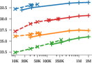
(a) PSNR

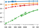
(b) SSIM

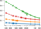
(c) LPIPS

Figure 16: Performance with different sizes and quality of the input point cloud. a, b, c) shows the PSNR, SSIM, and LPIPS [78] with different sizes of input point clouds (PSNR is repeated from the main paper). The solid and dashed lines represent the dense and coarse COLMAP reconstructions. The following scenes were evaluated (best to worst): tt/family, 360/room, tt/truck, and 360/garden from the Tanks and Temples [25] (tt) and the Mip-NeRF 360 [4] (360-indoor/360-outdoor) datasets. As expected, the quality increases with the number of points, but also sparse reconstruction performs better at the same number of points.

We conducted a study on the effect of different sizes of the input point cloud. In the main paper, we presented the PSNR results on four scenes. Here we also show the SSIM and LPIPS. We consider both the sparse and dense COLMAP reconstructions and analyse the performance as we sub-sample the points or add more points randomly. In order to save computational resources, we only train the method for $100$k iterations. The results are visualised in Figure 16.

As expected, the performance improves with the number of points used, as it leads to a finer subdivision of the scene around the surface. Note how the performance of dense reconstruction is lower than sparse reconstruction with the same size. Also, note how the performance of 360/garden increases when adding randomly sampled points to the sparse point cloud. For Tetra-NeRF it is important to have a dense-enough coverage in regions close to surfaces and randomly subsampling a larger point cloud may miss some regions. Similarly, adding more points at random in proximity to existing ones helps as it increases the density in those regions. For all experiments in the paper and the Supp. Mat., we used random sub-sampling. An interesting direction for future work is to investigate more sophisticated strategies that, e.g., sample more points around fine details such as corners and edges and fewer points in planar regions.

References

- [1] Kara-Ali Aliev, Artem Sevastopolsky, Maria Kolos, Dmitry Ulyanov, and Victor Lempitsky. Neural point-based graphics. In ECCV, 2020.
- [2] Pierre Alliez, Simon Giraudot, Clément Jamin, Florent Lafarge, Quentin Mérigot, Jocelyn Meyron, Laurent Saboret, Nader Salman, Shihao Wu, and Necip Fazil Yildiran. Point set processing. In CGAL User and Reference Manual. CGAL Editorial Board, 5.5.1 edition, 2022.
- [3] Jonathan T Barron, Ben Mildenhall, Matthew Tancik, Peter Hedman, Ricardo Martin-Brualla, and Pratul P Srinivasan. Mip-NeRF: A multiscale representation for anti-aliasing neural radiance fields. In ICCV, 2021.
- [4] Jonathan T Barron, Ben Mildenhall, Dor Verbin, Pratul P Srinivasan, and Peter Hedman. Mip-NeRF 360: Unbounded anti-aliased neural radiance fields. In CVPR, 2022.
- [5] Sai Bi, Zexiang Xu, Pratul Srinivasan, Ben Mildenhall, Kalyan Sunkavalli, Miloš Hašan, Yannick Hold-Geoffroy, David Kriegman, and Ravi Ramamoorthi. Neural reflectance fields for appearance acquisition. arXiv:2008.03824, 2020.
- [6] Wenjing Bian, Zirui Wang, Kejie Li, Jia-Wang Bian, and Victor Adrian Prisacariu. NoPe-NeRF: Optimising neural radiance field with no pose prior. arXiv:2212.07388, 2022.
- [7] Mark Boss, Raphael Braun, Varun Jampani, Jonathan T Barron, Ce Liu, and Hendrik Lensch. NeRD: Neural reflectance decomposition from image collections. In ICCV, 2021.
- [8] Chris Buehler, Michael Bosse, Leonard McMillan, Steven Gortler, and Michael Cohen. Unstructured lumigraph rendering. In Proceedings of the 28th annual conference on Computer graphics and interactive techniques, 2001.
- [9] Anpei Chen, Zexiang Xu, Andreas Geiger, Jingyi Yu, and Hao Su. TensoRF: Tensorial radiance fields. In ECCV, 2022.
- [10] Anpei Chen, Zexiang Xu, Xinyue Wei, Siyu Tang, Hao Su, and Andreas Geiger. Factor fields: A unified framework for neural fields and beyond. arXiv:2302.01226, 2023.
- [11] Anpei Chen, Zexiang Xu, Fuqiang Zhao, Xiaoshuai Zhang, Fanbo Xiang, Jingyi Yu, and Hao Su. MVSNeRF: Fast generalizable radiance field reconstruction from multi-view stereo. In ICCV, 2021.
- [12] Shuo Cheng, Zexiang Xu, Shilin Zhu, Zhuwen Li, Li Erran Li, Ravi Ramamoorthi, and Hao Su. Deep stereo using adaptive thin volume representation with uncertainty awareness. In CVPR, 2020.
- [13] Paul E Debevec, Camillo J Taylor, and Jitendra Malik. Modeling and rendering architecture from photographs: A hybrid geometry-and image-based approach. In Proceedings of the 23rd annual conference on Computer graphics and interactive techniques, 1996.
- [14] B Delaunay, S Vide, A Lamémoire, and V De Georges. Bulletin de l’academie des sciences de l’URSS. Classe des sciences mathématiques et naturelles, 6:793–800, 1934.
- [15] Boyang Deng, Jonathan T. Barron, and Pratul P. Srinivasan. JaxNeRF: an efficient JAX implementation of NeRF, 2020.
- [16] Michael S Floater. Generalized barycentric coordinates and applications. Acta Numerica, 24:161–214, 2015.
- [17] Sara Fridovich-Keil, Alex Yu, Matthew Tancik, Qinhong Chen, Benjamin Recht, and Angjoo Kanazawa. Plenoxels: Radiance fields without neural networks. In CVPR, 2022.
- [18] Yasutaka Furukawa and Jean Ponce. Accurate, dense, and robust multiview stereopsis. IEEE Transactions on Pattern Analysis and Machine Intelligence, 32:1362–1376, 2009.
- [19] Kaiming He, Xiangyu Zhang, Shaoqing Ren, and Jian Sun. Delving deep into rectifiers: Surpassing human-level performance on imagenet classification. In ICCV, 2015.
- [20] Peter Hedman, Julien Philip, True Price, Jan-Michael Frahm, George Drettakis, and Gabriel Brostow. Deep blending for free-viewpoint image-based rendering. SIGGRAPH, ToG, 37(6):1–15, 2018.
- [21] Peter Hedman, Pratul P Srinivasan, Ben Mildenhall, Jonathan T Barron, and Paul Debevec. Baking neural radiance fields for real-time view synthesis. In ICCV, 2021.
- [22] Vu Hoang Hiep, Renaud Keriven, Patrick Labatut, and Jean-Philippe Pons. Towards high-resolution large-scale multi-view stereo. In CVPR, 2009.
- [23] Michal Jancosek and Tomas Pajdla. Multi-view reconstruction preserving weakly-supported surfaces. In CVPR, 2011.
- [24] Michael Kazhdan, Matthew Bolitho, and Hugues Hoppe. Poisson surface reconstruction. In SGP, 2006.
- [25] Arno Knapitsch, Jaesik Park, Qian-Yi Zhou, and Vladlen Koltun. Tanks and temples: Benchmarking large-scale scene reconstruction. SIGGRAPH, ToG, 2017.
- [26] Georgios Kopanas, Julien Philip, Thomas Leimkühler, and George Drettakis. Point-based neural rendering with per-view optimization. In Computer Graphics Forum, volume 40, pages 29–43. Wiley Online Library, 2021.
- [27] Alex Krizhevsky, Ilya Sutskever, and Geoffrey E Hinton. Imagenet classification with deep convolutional neural networks. Advances in Neural Information Processing Systems, 25, 2012.
- [28] Jonáš Kulhánek, Erik Derner, Torsten Sattler, and Robert Babuška. ViewFormer: Nerf-free neural rendering from few images using transformers. In ECCV, 2022.
- [29] Patrick Labatut, Jean-Philippe Pons, and Renaud Keriven. Efficient multi-view reconstruction of large-scale scenes using interest points, Delaunay triangulation and graph cuts. In ICCV, 2007.
- [30] Patrick Labatut, J-P Pons, and Renaud Keriven. Robust and efficient surface reconstruction from range data. In Computer graphics forum, volume 28, pages 2275–2290. Wiley Online Library, 2009.
- [31] Chen-Hsuan Lin, Wei-Chiu Ma, Antonio Torralba, and Simon Lucey. BARF: Bundle-adjusting neural radiance fields. In ICCV, 2021.
- [32] Lingjie Liu, Jiatao Gu, Kyaw Zaw Lin, Tat-Seng Chua, and Christian Theobalt. Neural sparse voxel fields. Advances in Neural Information Processing Systems, 33:15651–15663, 2020.
- [33] Liyuan Liu, Haoming Jiang, Pengcheng He, Weizhu Chen, Xiaodong Liu, Jianfeng Gao, and Jiawei Han. On the variance of the adaptive learning rate and beyond. In International Conference on Learning Representations, 2020.
- [34] Stephen Lombardi, Tomas Simon, Jason Saragih, Gabriel Schwartz, Andreas Lehrmann, and Yaser Sheikh. Neural volumes: learning dynamic renderable volumes from images. SIGGRAPH, ToG, 38(4):1–14, 2019.
- [35] William E Lorensen and Harvey E Cline. Marching cubes: A high resolution 3D surface construction algorithm. SIGGRAPH, ToG, 1987.
- [36] Ricardo Martin-Brualla, Noha Radwan, Mehdi SM Sajjadi, Jonathan T Barron, Alexey Dosovitskiy, and Daniel Duckworth. NeRF in the wild: Neural radiance fields for unconstrained photo collections. In CVPR, 2021.
- [37] Nelson Max. Optical models for direct volume rendering. IEEE Transactions on Visualization and Computer Graphics, 1(2):99–108, 1995.
- [38] Moustafa Meshry, Dan B. Goldman, Sameh Khamis, Hugues Hoppe, Rohit Pandey, Noah Snavely, and Ricardo Martin-Brualla. Neural rerendering in the wild. In CVPR, June 2019.
- [39] Ben Mildenhall, Pratul P Srinivasan, Matthew Tancik, Jonathan T Barron, Ravi Ramamoorthi, and Ren Ng. NeRF: Representing scenes as neural radiance fields for view synthesis. In ECCV, 2020.
- [40] Tomas Möller. A fast triangle-triangle intersection test. Journal of Graphics Tools, 2(2):25–30, 1997.
- [41] Thomas Müller, Alex Evans, Christoph Schied, and Alexander Keller. Instant neural graphics primitives with a multiresolution hash encoding. SIGGRAPH, ToG, 2022.
- [42] M. Nießner, M. Zollhöfer, S. Izadi, and M. Stamminger. Real-time 3D reconstruction at scale using voxel hashing. SIGGRAPH, ToG, 2013.
- [43] Steven G Parker, James Bigler, Andreas Dietrich, Heiko Friedrich, Jared Hoberock, David Luebke, David McAllister, Morgan McGuire, Keith Morley, Austin Robison, et al. OptiX: a general purpose ray tracing engine. ACM Transactions on Graphics (ToG), 29(4):1–13, 2010.
- [44] Songyou Peng, Michael Niemeyer, Lars Mescheder, Marc Pollefeys, and Andreas Geiger. Convolutional occupancy networks. In ECCV, 2020.
- [45] Bui Tuong Phong. Illumination for computer generated pictures. Communications of the ACM, 18(6):311–317, 1975.
- [46] Ben Poole, Ajay Jain, Jonathan T Barron, and Ben Mildenhall. DreamFusion: Text-to-3D using 2D diffusion. arXiv:2209.14988, 2022.
- [47] Christian Reiser, Songyou Peng, Yiyi Liao, and Andreas Geiger. KiloNeRF: Speeding up neural radiance fields with thousands of tiny mlps. In ICCV, 2021.
- [48] Christian Reiser, Richard Szeliski, Dor Verbin, Pratul P Srinivasan, Ben Mildenhall, Andreas Geiger, Jonathan T Barron, and Peter Hedman. MERF: Memory-efficient radiance fields for real-time view synthesis in unbounded scenes. arXiv:2302.12249, 2023.
- [49] Jeremy Reizenstein, Roman Shapovalov, Philipp Henzler, Luca Sbordone, Patrick Labatut, and David Novotny. Common objects in 3D: Large-scale learning and evaluation of real-life 3D category reconstruction. In ICCV, 2021.
- [50] Gernot Riegler and Vladlen Koltun. Free view synthesis. In ECCV, 2020.
- [51] Gernot Riegler and Vladlen Koltun. Stable view synthesis. In CVPR, 2021.
- [52] Radu Alexandru Rosu and Sven Behnke. Permutosdf: Fast multi-view reconstruction with implicit surfaces using permutohedral lattices. In CVPR, 2023.
- [53] Darius Rückert, Linus Franke, and Marc Stamminger. ADOP: Approximate differentiable one-pixel point rendering. SIGGRAPH, ToG, 41(4):1–14, 2022.
- [54] Johannes Lutz Schönberger and Jan-Michael Frahm. Structure-from-motion revisited. In CVPR, 2016.
- [55] Johannes Lutz Schönberger, Enliang Zheng, Marc Pollefeys, and Jan-Michael Frahm. Pixelwise view selection for unstructured multi-view stereo. In ECCV, 2016.
- [56] Karen Simonyan and Andrew Zisserman. Very deep convolutional networks for large-scale image recognition. arXiv:1409.1556, 2014.
- [57] Cheng Sun, Min Sun, and Hwann-Tzong Chen. Direct voxel grid optimization: Super-fast convergence for radiance fields reconstruction. In CVPR, 2022.
- [58] Matthew Tancik, Vincent Casser, Xinchen Yan, Sabeek Pradhan, Ben Mildenhall, Pratul P Srinivasan, Jonathan T Barron, and Henrik Kretzschmar. Block-NeRF: Scalable large scene neural view synthesis. In CVPR, 2022.
- [59] Matthew Tancik, Pratul Srinivasan, Ben Mildenhall, Sara Fridovich-Keil, Nithin Raghavan, Utkarsh Singhal, Ravi Ramamoorthi, Jonathan Barron, and Ren Ng. Fourier features let networks learn high frequency functions in low dimensional domains. Advances in Neural Information Processing Systems, 33:7537–7547, 2020.
- [60] Matthew Tancik, Ethan Weber, Evonne Ng, Ruilong Li, Brent Yi, Justin Kerr, Terrance Wang, Alexander Kristoffersen, Jake Austin, Kamyar Salahi, et al. Nerfstudio: A modular framework for neural radiance field development. arXiv:2302.04264, 2023.
- [61] Chengzhou Tang and Ping Tan. BA-net: Dense bundle adjustment networks. In International Conference on Learning Representations, 2019.
- [62] Dor Verbin, Peter Hedman, Ben Mildenhall, Todd Zickler, Jonathan T Barron, and Pratul P Srinivasan. Ref-NeRF: Structured view-dependent appearance for neural radiance fields. In CVPR, 2022.
- [63] Sudheendra Vijayanarasimhan, Susanna Ricco, Cordelia Schmid, Rahul Sukthankar, and Katerina Fragkiadaki. SfM-Net: Learning of structure and motion from video. arXiv:1704.07804, 2017.
- [64] Can Wang, Menglei Chai, Mingming He, Dongdong Chen, and Jing Liao. Clip-NeRF: Text-and-image driven manipulation of neural radiance fields. In CVPR, 2022.
- [65] Peng Wang, Lingjie Liu, Yuan Liu, Christian Theobalt, Taku Komura, and Wenping Wang. NeuS: Learning neural implicit surfaces by volume rendering for multi-view reconstruction. Advances in Neural Information Processing Systems, 34:27171–27183, 2021.
- [66] Qianqian Wang, Zhicheng Wang, Kyle Genova, Pratul P. Srinivasan, Howard Zhou, Jonathan T. Barron, Ricardo Martin-Brualla, Noah Snavely, and Thomas Funkhouser. IBRNet: Learning multi-view image-based rendering. In CVPR, 2021.
- [67] Yiming Wang, Qin Han, Marc Habermann, Kostas Daniilidis, Christian Theobalt, and Lingjie Liu. NeuS2: Fast learning of neural implicit surfaces for multi-view reconstruction. arXiv:2212.05231, 2022.
- [68] Zirui Wang, Shangzhe Wu, Weidi Xie, Min Chen, and Victor Adrian Prisacariu. NeRF–: Neural radiance fields without known camera parameters. arXiv:2102.07064, 2021.
- [69] Daniel N Wood, Daniel I Azuma, Ken Aldinger, Brian Curless, Tom Duchamp, David H Salesin, and Werner Stuetzle. Surface light fields for 3D photography. In Proceedings of the 27th annual conference on Computer graphics and interactive techniques, 2000.
- [70] Qiangeng Xu, Zexiang Xu, Julien Philip, Sai Bi, Zhixin Shu, Kalyan Sunkavalli, and Ulrich Neumann. Point-NeRF: Point-based neural radiance fields. In CVPR, 2022.
- [71] Yao Yao, Zixin Luo, Shiwei Li, Tian Fang, and Long Quan. MVSNet: Depth inference for unstructured multi-view stereo. In ECCV, 2018.
- [72] Lior Yariv, Jiatao Gu, Yoni Kasten, and Yaron Lipman. Volume rendering of neural implicit surfaces. Advances in Neural Information Processing Systems, 34:4805–4815, 2021.
- [73] Lior Yariv, Peter Hedman, Christian Reiser, Dor Verbin, Pratul P Srinivasan, Richard Szeliski, Jonathan T Barron, and Ben Mildenhall. BakedSDF: Meshing neural SDFs for real-time view synthesis. arXiv:2302.14859, 2023.
- [74] Alex Yu, Ruilong Li, Matthew Tancik, Hao Li, Ren Ng, and Angjoo Kanazawa. PlenOctrees for real-time rendering of neural radiance fields. In ICCV, 2021.
- [75] Alex Yu, Vickie Ye, Matthew Tancik, and Angjoo Kanazawa. PixelNeRF: Neural radiance fields from one or few images. In CVPR, 2021.
- [76] Zehao Yu, Songyou Peng, Michael Niemeyer, Torsten Sattler, and Andreas Geiger. MonoSDF: Exploring monocular geometric cues for neural implicit surface reconstruction. In Advances in Neural Information Processing Systems, 2022.
- [77] Kai Zhang, Gernot Riegler, Noah Snavely, and Vladlen Koltun. NeRF++: Analyzing and improving neural radiance fields. arXiv:2010.07492, 2020.
- [78] Richard Zhang, Phillip Isola, Alexei A. Efros, Eli Shechtman, and Oliver Wang. The unreasonable effectiveness of deep features as a perceptual metric. In CVPR, June 2018.
- [79] Chaoqiang Zhao, Qiyu Sun, Chongzhen Zhang, Yang Tang, and Feng Qian. Monocular depth estimation based on deep learning: An overview. Science China Technological Sciences, 63(9):1612–1627, 2020.