Gluon distributions in the proton in a light-front spectator model

Abstract

We formulate a light-front spectator model for the proton incorporating the gluonic degree of freedom. In this model, at high energy scattering of the proton, the active parton is a gluon and the rest is viewed as a spin-$\frac{1}{2}$ spectator with an effective mass. The light front wave functions of the proton are constructed using a soft wall AdS/QCD prediction and parameterized by fitting the unpolarized gluon distribution function to the NNPDF3.0nlo data set. We investigate the helicity distribution of gluon in this model. We find that our prediction for the gluon helicity asymmetry agrees well with existing experimental data and satisfies the perturbative QCD constraints at small and large longitudinal momentum regions. We also present the transverse momentum dependent distributions (TMDs) for gluon in this model. We further show that the model-independent Mulders-Rodrigues inequalities are obeyed by the TMDs computed in our model.

I Introduction

Understanding the structure of hadrons in terms of the fundamental degrees of freedom in QCD i.e., quarks and gluons, is one of the remaining challenges in nuclear and particle physics. There have been numerous research in recent years to learn more about the parton distributions (PDFs), transverse momentum dependent distributions (TMDs), generalized parton distributions (GPDs), gravitational form factors (GFFs), Wigner distributions, etc., of the quarks and their properties were investigated using various theoretical models Meissner et al. (2007); Jakob et al. (1997); Brodsky et al. (2002); Bacchetta et al. (2008); Pasquini et al. (2008); Maji and Chakrabarti (2017); Gurjar et al. (2021, 2022); Lorce and Pasquini (2011); Ji et al. (1997); Scopetta and Vento (2003); Boffi et al. (2003, 2004); Vega et al. (2011); Chakrabarti and Mondal (2013); Mondal and Chakrabarti (2015); Chakrabarti and Mondal (2015); Xu et al. (2021); Kriesten et al. (2022); Chakrabarti et al. (2016); Meissner et al. (2008, 2009); Burkert et al. (2023), revealing numerous insights into the nucleon structure. In comparison to quark distributions, the gluon distributions are less precisely known, which has an impact on the calculation of the cross-section of a process dominated by the gluon-initiated channel. Gluons, which mediate the strong interaction, play a crucial role in the mass and spin of the nucleon Ji et al. (2021); Jaffe and Manohar (1990); Ji (1997); Leader (2022); Liu and Lorcé (2016). In the study of deep inelastic scattering processes, the gluon distributions and fragmentation functions contain essential information about the system Xie and Lu (2022). These process-independent distributions characterize the soft part of the scattering, or the deep structure of the hadrons, together with their quark and antiquark equivalents. The majority of hadron high energy scattering investigations relies on the QCD factorization, in which PDFs play a crucial role. There are two gluonic PDFs at leading twist: unpolarized $f_{1}^{g}(x)$ and polarized $g_{1L}^{g}(x)$ PDFs. The unpolarized gluon PDF has been studied using lattice QCD Khan et al. (2021); Yang et al. (2017); Delmar et al. (2022); Sufian et al. (2021) and various other theoretical approaches Brodsky et al. (2001); Dosch et al. (2022); Hou et al. (2021); Ball et al. (2017); Delmar et al. (2022); Freese et al. (2021) with better accuracy as compared to the polarized PDF. The uncertainty is mainly in the small $x$ region of the polarized PDF. Even the sign of the polarized PDF in the small $x$ region is not yet well-decided de Florian et al. (2014).

The first Mellin moment of the gluon polarized PDF gives the gluon spin contribution to the proton spin. It is found that the quark spin only contributes around $(20-30)\%$ of the proton spin Ashman et al. (1988, 1989); de Florian et al. (2009); Nocera et al. (2014); Ethier et al. (2017). Even after separating out the quark OAM and spin contributions, there is a sizable amount of spin contribution that can not be explained through quarks only. Several experiments like the RHIC spin program at BNL Nocera et al. (2014); Ethier et al. (2017); de Florian et al. (2014), PHENIX Adare et al. (2014, 2009) and COMPASS Adolph et al. (2016) observed a non-zero gluon helicity suggesting that the proton spin is significantly influenced by the gluon, which is important to resolve the proton spin puzzle. However, the gluon helicity is not well determined yet. The polarized PDF $g_{1L}^{g}(x)$ measures the gluon spin contribution to the proton but it has large uncertainty in the small-$x$ region. Recently, some theoretical studies using the basis light-front quantization (BLFQ) approach Xu et al. (2022), the holographic light-front QCD (HLFQCD) approach Gurjar et al. (2023), and the lattice QCD Khan et al. (2022); Egerer et al. (2022); Sufian et al. (2021) have reported the nonzero and sizeable contributions of the gluon spin to the total proton spin. While there have been significant improvements in the extracted $g_{1L}^{g}(x)$ precision over the last decade Gehrmann and Stirling (1996); Gluck et al. (2001); Blumlein and Bottcher (2002), there are still various concerns, such as the suppression in the gluon distribution in the momentum fraction region $0.1<x<0.4$ when the ATLAS and CMS jet data are included Hou et al. (2021), determination of gluon helicity in entire $x$-region etc. Accurate measurement of the nucleon spin structure, specifically the gluon and sea quark distributions, are two of the primary scientific objectives of the forthcoming Electron-Ion-Colliders (EICs) Accardi et al. (2016); Abdul Khalek et al. (2022); Anderle et al. (2021). It is not yet completely clear how gluons, valence quarks, and sea quarks share the mass and the spin of the proton. But in recent studies, it has been found that gluons contribute more to the proton spin than the valence quarks. The Electron-Ion-Collider (EIC) will focus particularly on the small-$x$ region, which contains more gluon density and is complicated to study. Also, the gluons play a crucial role in determining the mass of the proton, as their interactions with quarks contribute significantly to the overall mass of the proton Ji (1995a, b). Understanding the role of gluons in proton mass decomposition is an active area of research in theoretical and experimental physics, and has important implications for our understanding of the fundamental building blocks of matter Burkert et al. (2023); Rodini et al. (2020); Metz et al. (2020); Lorcé et al. (2021).

In addition to PDFs, we also explore the gluon TMDs in this work. It has recently been demonstrated that gluons and quark TMDs are essential to describe the three-dimensional picture of the nucleon in momentum space. The gluon TMDs have been studied in D’Alesio et al. (2019); Mulders and Rodrigues (2001); Boer et al. (2016); Lyubovitskij and Schmidt (2021a); Bacchetta et al. (2020); Lu and Ma (2016). TMDs play a crucial role in the experimentally observed single spin and azimuthal asymmetries in for example semi-inclusive deep inelastic scattering (SIDIS) and Drell-Yan (DY) processes. There are eight leading twist gluon TMDs. The collinear limit of the TMDs $f_{1}^{g}(x,{\bf p}_{\perp}^{2})$ and $g_{1L}^{g}(x,{\bf p}_{\perp}^{2})$ are related to the unpolarized and polarized PDFs, respectively. An overview of the available literature on unpolarized and helicity gluon TMDs at small-$x$ can be found in Ref. Petreska (2018) (and references therein). Some recent theoretical and phenomenological studies are discussed in Refs. Altinoluk et al. (2019, 2020); Zhou (2019).

Recently, a few spectator models have been proposed for the study of the gluon distributions Bacchetta et al. (2020); Lyubovitskij and Schmidt (2021b); Lu and Ma (2016); Tan and Lu (2023). In the construction of the spectator models, the crucial step is the choice of the light-front wave functions Brodsky et al. (2001). We can write the form factors, PDFs, TMDs, GPDs and Wigner distributions in terms of the light-front wave functions in a spectator model. It has been verified that the form factors and partonic distributions follow model-independent scaling rules in the limiting cases of the longitudinal momentum fraction $x$. The behaviour of gluon parton densities at large and small $x$ have been observed in Refs. Brodsky and Schmidt (1990); Brodsky et al. (1995). In these works, the authors derived QCD constraints  Brodsky and Schmidt (1990) on unpolarized $f_{1}^{g}$, polarized $g_{1L}^{g}$ gluon PDFs and on the gluon helicity asymmetry ratio $g_{1L}^{g}/f_{1}^{g}$, which goes to zero as $x\to 0$ and it is 1 as $x\to 1$ . A reasonably good model should follow these limiting conditions. In this work, we study the gluon PDFs and T-even gluon TMDs using a light-front gluon spectator model, where the light-front wave functions are constructed using a soft wall AdS/QCD prediction Brodsky et al. (2015). This model is a generalization of the light-front quark-diquark model Gutsche et al. (2014); Maji and Chakrabarti (2016); Mondal and Chakrabarti (2015). The gluon-spectator model describes the nucleon as a composite system of an active gluon and the rest of the system as a spectator. At low energy, the spectator contains mainly three valence quarks of the nucleon. We are considering the spectator as a spin-$\frac{1}{2}$ effective system.

The paper is organized as follows: In Sec. II, we discuss about our model construction. We show the model calculation of the T-even TMDs in Sec. III. In Sec. IV, we determine our model parameters from the fitting of our unpolarized gluon PDF to the NNPDF3.0nlo data. In Sec. V, we show our model results for all four T-even gluon TMDs. Finally, we provide a brief summary and discussion in Sec. VI.

II Model construction

The minimum Fock state of the proton contains only valence quarks. As we include the higher Fock sectors then gluons, and sea quarks also come into the picture. In this simplified model, we describe the proton as a composite state of one active gluon and a spin-$\frac{1}{2}$ spectator Lu and Ma (2016).

We choose a reference frame in which the transverse momentum of the proton vanishes, i.e. $P=(P^{+},\frac{M^{2}}{P^{+}},\textbf{0}_{\perp})$. The momentum of the active parton is given by $p=(xP^{+},\frac{p^{2}+\textbf{p}_{\perp}^{2}}{xP^{+}},\textbf{p}_{\perp})$ and the momentum of the spectator $P_{X}=((1-x)P^{+},P^{-}_{X},-\textbf{p}_{\perp})$ with $x=p^{+}/P^{+}$ being the fraction of proton longitudinal momentum carried by the struck gluon. The proton state can be written as a two-particle Fock-state expansion with proton spin components $J_{z}=\pm\frac{1}{2}$ Brodsky et al. (2001) as,

$$|P;\uparrow(\downarrow)\rangle=\int\frac{\mathrm{d}^{2}{\bf p}_{\perp}\mathrm{d}x}{16\pi^{3}\sqrt{x(1-x)}}\times\Bigg{[}\psi_{+1+\frac{1}{2}}^{\uparrow(\downarrow)}\left(x,{\bf p}_{\perp}\right)\left|+1,+\frac{1}{2};xP^{+},{\bf p}_{\perp}\right\rangle+\psi_{+1-\frac{1}{2}}^{\uparrow(\downarrow)}\left(x,{\bf p}_{\perp}\right)\left|+1,-\frac{1}{2};xP^{+},{\bf p}_{\perp}\right\rangle$$

$$+\psi_{-1+\frac{1}{2}}^{\uparrow(\downarrow)}\left(x,{\bf p}_{\perp}\right)\left|-1,+\frac{1}{2};xP^{+},{\bf p}_{\perp}\right\rangle+\psi_{-1-\frac{1}{2}}^{\uparrow(\downarrow)}\left(x,{\bf p}_{\perp}\right)\left|-1,-\frac{1}{2};xP^{+},{\bf p}_{\perp}\right\rangle\bigg{]},$$ (1)

where $\psi_{\lambda_{g}\lambda_{X}}^{\uparrow(\downarrow)}(x,{\bf p}_{\perp})$ are the LFWFs corresponding to the two-particle state $|\lambda_{g},\lambda_{X};xP^{+},{\bf p}_{\perp}\rangle$ with proton helicities $\lambda_{p}=\uparrow(\downarrow)$. Here, $\lambda_{g}$ and $\lambda_{X}$ stand for the helicity components of the constituent gluon and spectator, respectively.

Our proposal for the light-front wave functions in Eq. (II) is inspired by the wave function of the physical electron  Brodsky et al. (2001), which is made up of a spin-1 photon and a spin-$\frac{1}{2}$ electron. We argue that the light-front wave functions for the Fock-state expansion for a proton with $J_{z}=+1/2$ have the following form:

$$\psi_{+1+\frac{1}{2}}^{\uparrow}\left(x,{\bf p}_{\perp}\right) = -\sqrt{2}\frac{(-p^{1}_{\perp}+ip^{2}_{\perp})}{x(1-x)}\varphi(x,{\bf p}_{\perp}^{2}),$$

$$\psi_{+1-\frac{1}{2}}^{\uparrow}\left(x,{\bf p}_{\perp}\right) = -\sqrt{2}\bigg{(}M-\frac{M_{X}}{(1-x)}\bigg{)}\varphi(x,{\bf p}_{\perp}^{2}),$$

$$\psi_{-1+\frac{1}{2}}^{\uparrow}\left(x,{\bf p}_{\perp}\right) = -\sqrt{2}\frac{(p^{1}_{\perp}+ip^{2}_{\perp})}{x}\varphi(x,{\bf p}_{\perp}^{2}),$$

$$\psi_{-1-\frac{1}{2}}^{\uparrow}\left(x,{\bf p}_{\perp}\right) = 0,$$ (2)

where $M$ and $M_{X}$ represent the masses of the proton and spectator, respectively. $\varphi(x,{\bf p}_{\perp}^{2})$ is the modified form of the soft-wall AdS/QCD wave function Gutsche et al. (2014) modeled by introducing the parameters $a$ and $b$. Similarly, the light-front wave functions for the proton with $J_{z}=-1/2$ have the form

$$\psi_{+1+\frac{1}{2}}^{\downarrow}\left(x,{\bf p}_{\perp}\right) = 0,$$

$$\psi_{+1-\frac{1}{2}}^{\downarrow}\left(x,{\bf p}_{\perp}\right) = -\sqrt{2}\frac{(-p^{1}_{\perp}+ip^{2}_{\perp})}{x}\varphi(x,{\bf p}_{\perp}^{2}),$$

$$\psi_{-1+\frac{1}{2}}^{\downarrow}\left(x,{\bf p}_{\perp}\right) = -\sqrt{2}\bigg{(}M-\frac{M_{X}}{(1-x)}\bigg{)}\varphi(x,{\bf p}_{\perp}^{2}),$$

$$\psi_{-1-\frac{1}{2}}^{\downarrow}\left(x,{\bf p}_{\perp}\right) = -\sqrt{2}\frac{(p^{1}_{\perp}+ip^{2}_{\perp})}{x(1-x)}\varphi(x,{\bf p}_{\perp}^{2}).$$ (3)

The behaviour at $x\rightarrow 0$, as well as the counting rules at $x\rightarrow 1$, provide information on the various gluon distributions  Brodsky and Schmidt (1990); Brodsky et al. (1995). To elaborate, the asymptotic behaviour of the PDFs at small $x$ is adopted from the observed Regge behaviour in particle colliders, and the large-$x$ behavior is based on the power counting rules for hard scattering Brodsky et al. (1995). Keeping all these in mind, we have modified the soft wall AdS-QCD wave function, $\varphi(x,{\bf p}_{\perp}^{2})$, The complete form of the modified soft-wall AdS/QCD wave function is given by,

$$\varphi(x,{\bf p}_{\perp}^{2})=N_{g}\frac{4\pi}{\kappa}\sqrt{\frac{\log[1/(1-x)]}{x}}x^{b}(1-x)^{a}\exp{\bigg{[}-\frac{\log[1/(1-x)]}{2\kappa^{2}x^{2}}{\bf p}_{\perp}^{2}\bigg{]}}.$$ (4)

where $a$ and $b$ are our model parameters. The values of the model parameters $a$, $b$, and the normalization constant $N_{g}$ are fixed by fitting the gluon unpolarized PDF at the scale $\mu_{0}=2$ GeV with NNPDF3.0 data. For the stability of the proton, the spectator mass, $M_{X}$ is considered higher than the proton mass i.e., $M_{X}>M$.

III Gluon TMDs

In the light front formalism, the unintegrated gluon correlation function for leading twist gluon TMDs in the SIDIS process is given by the following relation Mulders and Rodrigues (2001):

$$\Phi^{g[ij]}(x,{\bf p}_{\perp};S)=\frac{1}{xP^{+}}\int\frac{d\xi^{-}}{2\pi}\,\frac{d^{2}\mathbf{\xi}{{}_{\perp}}}{(2\pi)^{2}}\,e^{ik\cdot\xi}\,\big{<}P;S\big{|}\,F^{+j}_{a}(0)\ \,\mathcal{W}_{+\infty,ab}(0;\xi)\,F^{+i}_{b}(\xi)\,\big{|}P;S\big{>}\,\Big{|}_{\xi^{+}=0^{+}}\,,$$ (5)

where $F^{\mu\nu}$ is the gluon field strength tensor and $\mathcal{W}_{+\infty,ab}$ is the Wilson line that ensures the correlator to be gauge invariant. The subscript “$+$” specifies that the Wilson line in the correlator operator expression is future-pointing, which is necessary for SIDIS TMD distributions. There are eight leading twist gluon TMDs out of which four of them are T-even ($f_{1}^{g}$, $g_{1L}^{g}$, $g_{1T}^{g}$, and $h_{1}^{\perp g}$) and the remaining four are T-odd ($f_{1T}^{\bot g},\;h_{1L}^{\bot g},\;h_{1T}^{g},\;h_{1T}^{\bot g}$) Meissner et al. (2007); Mulders and Rodrigues (2001). The twist-2 gluon TMDs are defined through the correlator (5) as Meissner et al. (2007)

$$\Phi^{g}(x,{\bf p}_{\perp};S) = \delta_{T}^{ij}\,\Phi^{g[ij]}(x,{\bf p}_{\perp};S)$$

$$= f_{1}^{g}(x,{\bf p}_{\perp}^{2})-\frac{\epsilon^{ij}_{\perp}{\bf p}_{\perp}^{i}S_{\perp}^{j}}{M}\,f_{1T}^{\bot g}(x,{\bf p}_{\perp}^{\,2})\,,$$

$$\tilde{\Phi}^{g}(x,{\bf p}_{\perp};S) = i\epsilon_{T}^{ij}\,\Phi^{g[ij]}(x,{\bf p}_{\perp};S)$$

$$= \lambda\,g_{1L}^{g}(x,{\bf p}_{\perp}^{\,2})+\frac{{\bf p}_{\perp}\cdot\mathbf{S}_{\perp}}{M}\,g_{1T}^{g}(x,{\bf p}_{\perp}^{\,2})\,,$$

$$\Phi_{T}^{g,\,ij}(x,{\bf p}_{\perp};S) =-\boldsymbol{\hat{S}}\,\Phi^{g[ij]}(x,{\bf p}_{\perp};S)$$ (8)

$$=-\frac{\hat{\mathbf{S}}{\bf p}_{\perp}^{i}{\bf p}_{\perp}^{j}}{2M^{2}}\,h_{1}^{\perp g}(x,{\bf p}_{\perp}^{2})+\frac{\lambda\,\boldsymbol{\hat{S}}{\bf p}_{\perp}^{i}\epsilon_{\perp}^{jk}{\bf p}_{\perp}^{k}}{2M^{2}}\,h_{1L}^{\perp g}(x,{\bf p}_{\perp}^{2})$$

$$+\frac{\hat{\bm{S}}{\bf p}_{\perp}^{i}\epsilon_{\perp}^{jk}S_{\perp}^{k}}{2M}\,\bigg{(}h_{1T}^{g}(x,{\bf p}_{\perp}^{\,2})+\frac{{\bf p}_{\perp}^{\,2}}{2M^{2}}\,h_{1T}^{\bot g}(x,{\bf p}_{\perp}^{\,2})\bigg{)}$$

$$+\frac{\hat{\bm{S}}{\bf p}_{\perp}^{i}\epsilon_{\perp}^{jk}\big{(}2p_{\perp}^{k}{\bf p}_{\perp}.\mathbf{S}_{\perp}-S_{\perp}^{k}{\bf p}_{\perp}^{\,2}\big{)}}{4M^{3}}h_{1T}^{\perp g}(x,{\bf p}_{\perp}^{2}).$$

Using the above Eqs. (III)-(8), one can compute all the T-even TMDs. The unpolarized TMD, $f_{1}^{g}(x,{\bf p}_{\perp}^{2})$ is defined as the overlap representation of the proton light-front wave functions as More et al. (2018)

$$f_{1}^{g}(x,{\bf p}_{\perp}^{2}) = \frac{1}{16\pi^{3}}\sum_{\lambda_{g}\lambda_{X}}(\epsilon^{1\ast}_{\lambda_{g}}\epsilon^{1}_{\lambda_{g}}+\epsilon^{2\ast}_{\lambda_{g}}\epsilon^{2}_{\lambda_{g}})\psi_{\lambda_{g}\lambda_{X}}^{\uparrow\ast}(x,{\bf p}_{\perp}^{2})\psi_{\lambda_{g}\lambda_{X}}^{\uparrow}(x,{\bf p}_{\perp}^{2})$$ (9)

$$= \frac{1}{16\pi^{3}}\bigg{[}|\psi_{+1+1/2}^{\uparrow}(x,{\bf p}_{\perp}^{2})|^{2}+|\psi_{+1-1/2}^{\uparrow}(x,{\bf p}_{\perp}^{2})|^{2}+|\psi_{-1+1/2}^{\uparrow}(x,{\bf p}_{\perp}^{2})|^{2}\bigg{]}.$$

After employing the light-front wave functions, Eqs. (II) and (II) in the above Eq. (9), we obtain the gluon unpolarized TMD as,

$$f_{1}^{g}(x,{\bf p}_{\perp}^{2})=N_{g}^{2}\frac{2}{\pi\kappa^{2}}\frac{\log[1/(1-x)]}{x}x^{2b}(1-x)^{2a}\bigg{[}A(x)+{\bf p}_{\perp}^{2}B(x)\bigg{]}\exp[-C(x){\bf p}_{\perp}^{2}],$$ (10)

where $A(x)$, $B(x)$ and $C(x)$ are given by

$$A(x)=\bigg{(}M-\frac{M_{X}}{(1-x)}\bigg{)}^{2},\hskip 14.22636ptB(x)=\frac{1+(1-x)^{2}}{x^{2}(1-x)^{2}}\hskip 14.22636pt\text{and}\hskip 14.22636ptC(x)=\frac{\log[1/(1-x)]}{\kappa^{2}x^{2}}.$$ (11)

Similarly, the gluon helicity TMD $g_{1L}^{g}(x,{\bf p}_{\perp}^{2})$, which describes the distribution of a circularly polarised gluon in a longitudinally polarised proton, is defined as

$$g_{1L}^{g}(x,{\bf p}_{\perp}^{2}) = \frac{1}{16\pi^{3}}i\sum_{\lambda_{g}\lambda_{X}}(\epsilon^{2\ast}_{\lambda_{g}}\epsilon^{1}_{\lambda_{g}}-\epsilon^{1\ast}_{\lambda_{g}}\epsilon^{2}_{\lambda_{g}})\psi_{\lambda_{g}\lambda_{X}}^{\uparrow\ast}(x,{\bf p}_{\perp}^{2})\psi_{\lambda_{g}\lambda_{X}}^{\uparrow}(x,{\bf p}_{\perp}^{2})$$ (12)

$$= \frac{1}{16\pi^{3}}\bigg{[}|\psi_{+1+1/2}^{\uparrow}(x,{\bf p}_{\perp}^{2})|^{2}+|\psi_{+1-1/2}^{\uparrow}(x,{\bf p}_{\perp}^{2})|^{2}-|\psi_{-1+1/2}^{\uparrow}(x,{\bf p}_{\perp}^{2})|^{2}\bigg{]}.$$ (13)

The analytical expression for the gluon helicity TMD in our model is obtained as,

$$g_{1L}^{g}(x,{\bf p}_{\perp}^{2})=N_{g}^{2}\frac{2}{\pi\kappa^{2}}\frac{\log[1/(1-x)]}{x}x^{2b}(1-x)^{2a}\bigg{[}A(x)+{\bf p}_{\perp}^{2}\tilde{B}(x)\bigg{]}\exp[-C(x){\bf p}_{\perp}^{2}],$$ (14)

where $A(x)$, $C(x)$ are same as (11), while $\tilde{B}(x)$ is given as

$$\tilde{B}(x) = \frac{1-(1-x)^{2}}{x^{2}(1-x)^{2}}.$$ (15)

The worm-gear gluon TMD $g_{1T}^{g}(x,{\bf p}_{\perp}^{2})$ is defined as the distribution of a circularly polarised gluon in a transversely polarized proton Lyubovitskij and Schmidt (2021b) and given by,

$$\frac{{\bf p}_{\perp}.\mathbf{S_{\perp}}}{M}g_{1T}^{g}(x,{\bf p}_{\perp}^{2}) = \frac{1}{16\pi^{3}}\frac{i}{2}\sum_{\lambda_{g}\lambda_{X}}(\epsilon^{1\ast}_{\lambda_{g}}\epsilon_{\lambda_{g}}^{2}-\epsilon^{2\ast}_{\lambda_{g}}\epsilon^{1}_{\lambda_{g}})\bigg{[}\psi_{\lambda_{g}\lambda_{X}}^{\uparrow\ast}(x,{\bf p}_{\perp})\psi_{\lambda_{g}\lambda_{X}}^{\downarrow}(x,{\bf p}_{\perp})+\psi_{\lambda_{g}\lambda_{X}}^{\downarrow\ast}(x,{\bf p}_{\perp})\psi_{\lambda_{g}\lambda_{X}}^{\uparrow}(x,{\bf p}_{\perp})\bigg{]}$$

$$g_{1T}^{g}(x,{\bf p}_{\perp}^{2}) = -\frac{4M}{16\pi^{3}x}\bigg{(}M-\frac{M_{X}}{(1-x)}\bigg{)}[\varphi(x,{\bf p}_{\perp}^{2})]^{2}.$$ (16)

Using the soft-wall AdS/QCD wave function (4), the above equation can be written as,

$$g_{1T}^{g}(x,{\bf p}_{\perp}^{2}) = -\frac{4M}{\pi\kappa^{2}}N_{g}^{2}\bigg{(}M(1-x)-{M_{X}}\bigg{)}\log[1/(1-x)]x^{2b-2}(1-x)^{2a-1}\exp[-C(x){\bf p}_{\perp}^{2}].$$ (17)

Finally, The Boer-Mulders gluon TMD $h_{1}^{\perp g}(x,{\bf p}_{\perp}^{2})$, which describes a linearly polarized gluon inside an unpolarized proton, is given as,

$$\frac{{\bf p}_{\perp}^{2}}{2M^{2}}h_{1}^{\perp g}(x,{\bf p}_{\perp}^{2}) = -\frac{1}{2}\sum_{\lambda_{N}\lambda_{g}\neq\lambda_{g}^{\prime}\lambda_{X}}\frac{1}{16\pi^{3}}\Big{[}\psi_{\lambda_{g}^{\prime}\lambda_{X}}^{\star\lambda_{N}}(x,{\bf p}_{\perp})\psi_{\lambda_{g}\lambda_{X}}^{\lambda_{N}}(x,{\bf p}_{\perp})\epsilon^{\mu\dagger}_{\lambda_{g}^{\prime}}\epsilon^{\nu}_{\lambda_{g}}\Big{]},\,$$

$$h_{1}^{\perp g}(x,{\bf p}_{\perp}^{2}) = -\frac{1}{16\pi^{3}}\frac{M^{2}}{{\bf p}_{\perp}^{4}}\sum_{\lambda_{N}\lambda_{X}}\bigg{[}(p^{1}-ip^{2})^{2}\psi_{+1\lambda_{X}}^{\star\lambda_{N}}(x,{\bf p}_{\perp})\psi_{-1\lambda_{X}}^{\lambda_{N}}(x,{\bf p}_{\perp})+(p^{1}+ip^{2})^{2}\psi_{-1\lambda_{X}}^{\star\lambda_{N}}(x,{\bf p}_{\perp})\psi_{+1\lambda_{X}}^{\lambda_{N}}(x,{\bf p}_{\perp})\bigg{]}$$

$$= \frac{8M^{2}}{16\pi^{3}}\frac{1}{x^{2}(1-x)}[\varphi(x,{\bf p}_{\perp}^{2})]^{2},$$

$$h_{1}^{\perp g}(x,{\bf p}_{\perp}^{2}) = \frac{8M^{2}}{\pi\kappa^{2}}N_{g}^{2}\log[1/(1-x)]x^{2b-3}(1-x)^{2a-1}\exp[-C(x){\bf p}_{\perp}^{2}].$$

After performing the ${\bf p}_{\perp}$-integration of the gluon unpolarized TMD, Eq. (10), we obtain the corresponding collinear unpolarized PDF, $f_{1}^{g}(x)$ as,

$$f_{1}^{g}(x) = \int d^{2}{\bf p}_{\perp}f_{1}^{g}(x,{\bf p}_{\perp}^{2})$$

$$= 2N_{g}^{2}x^{2b+1}(1-x)^{2a-2}\bigg{[}\kappa^{2}\frac{(1+(1-x)^{2})}{\log[1/(1-x)]}+(M(1-x)-M_{x})^{2}\bigg{]}.$$

The gluon helicity PDF $g_{1L}^{g}(x)$ can be obtained after the ${\bf p}_{\perp}$-integration of the gluon helicity TMD in Eq. (14) as,

$$g_{1L}^{g}(x) = \int d^{2}{\bf p}_{\perp}g_{1L}^{g}(x,{\bf p}_{\perp}^{2})$$

$$= 2N_{g}^{2}x^{2b+1}(1-x)^{2a-2}\bigg{[}\kappa^{2}\frac{(1-(1-x)^{2})}{\log[1/(1-x)]}+(M(1-x)-M_{x})^{2}\bigg{]}.$$

Similarly, the collinear PDFs of worm-gear, Eq.(17), and the Boer-Mulders, Eq.(III), TMDs are given as,

$$g_{1T}^{g}(x) = \int d^{2}{\bf p}_{\perp}g_{1T}^{g}(x,{\bf p}_{\perp}^{2})$$

$$= 4MN_{g}^{2}\big{(}M(1-x)-M_{x}\big{)}x^{2b}(1-x)^{2a-1},$$

and,

$$h_{1}^{\perp g}(x) = \int d^{2}{\bf p}_{\perp}h_{1}^{\perp g}(x,{\bf p}_{\perp}^{2})$$

$$= 8MN_{g}^{2}x^{2b-1}(1-x)^{2a-1}.$$

IV Numerical fitting and model parameters

There are four parameters $a$, $b$, $N_{g}$, and $M_{X}$ in our model, which will decide the goodness of the model. The parameters $N_{g}$ and $M_{X}$ are free parameters and they are fixed by normalization conditions of the gluon PDFs and spectator mass properties of the proton, respectively. The parameters $a$ and $b$ decide the behaviour of the distributions in extreme limits of $x$ are crucial to fix. We determine these model parameters, by fitting our unpolarized gluon distribution with the latest available gluon PDF data at NLO of the gluon distribution $xf_{1}^{g}(x)$ from the global analysis by the NNPDF Collaboration Ball et al. (2017). We particularly fit NNPDF3.0 NLO unpolarized gluon distribution at the scale $Q_{0}=2$ GeV. We choose 300 data points within the interval $0.001<x<1$ and 100 replicas of the gluon distribution. The effective uncertainties are calculated from the standard deviation of these 100 replicas for each value of $x_{i}$.

We set the gluon mass $M_{g}=0$. The choice of model parameters $a$ and $b$ depend on the spectator mass. During the search for the optimal fit, we find that for spectator mass close to the proton mass, the model parameters produce a more physically acceptable spin contribution of the gluon than for larger spectator mass. Here, we choose $M_{X}=0.985$ GeV. In a similar kind of spectator model, the spectator mass has been chosen as $M_{x}=0.943$ Lu and Ma (2016). The model is very sensitive in the small $x$ region. Even in the NNPDF analysis, the polarised PDF has large uncertainty in the small-$x$ region, which makes the spin contribution prediction sensitive to the lower limit of $x$. Keeping all of this in mind, we exclude a very small $x$ region from our fitting and our model is valid for the range $0.001<x<1$.

The value of the fitted model parameters is listed in Table 1.

Table 1: Numerical values and the uncertainties of the fitted model parameters $a$ and $b$.

Parameter	Central Value	$1\sigma$-Error band	$2\sigma$-Error band
$a$	3.88	$\pm$ 0.1020	$\pm$ 0.2232
$b$	-0.53	$\pm$ 0.0035	$\pm$ 0.0071

These model parameters are fixed by fitting the NNPDF3.0 NLO data set at $\mu^{2}=4$ GeV² with a $\chi_{\rm min}^{2}=20.37$ with the normalization constant $N_{g}=2.088$. We notice that the $2\sigma$ uncertainty to the parameter fitting is close to the experimental error corridor, and we take $2\sigma$ uncertainty as a standard maximized error in this model for further reporting. The parameters in the wave functions determined by the fitting of unpolarized gluon PDF can be further employed to predict the other gluon distributions e.g., gluon helicity, transversity, TMDs etc. In Fig. 1, we show the results of our fit for the unpolarized gluon distribution $xf_{1}^{g}(x)$ at $Q_{0}=2$ GeV. The solid magenta band identifies the NNPDF3.0 parametrization of $xf_{1}^{g}(x)$ Ball et al. (2018) and the blue-dashed line with the blue band shows our model results at $2\sigma$ error corridor.

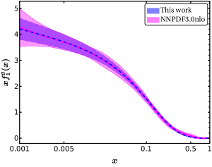
Figure 1: Our model Unpolarized gluon PDF $f_{1}^{g}(x)$ (blue dashed line with blue band of $2\sigma$ error) compared with the NNPDF3.0nlo data set (solid magenta line with magenta band) as a function of longitudinal momentum fraction $x$ in the kinematics region $0.001\leq x\leq 1$ at $Q_{0}=2$GeV.

V Results

The value of the average longitudinal momentum of the gluon is defined as the second Mellin’s moment of the unpolarized PDF as,

$$\langle x\rangle_{g}=\int_{0}^{1}dxxf_{1}^{g}(x)=0.416^{+0.048}_{-0.041},$$ (22)

which is close to the recent lattice calculations at $Q^{2}=4$ GeV², $\langle x\rangle_{g}=0.427(92)$ Alexandrou et al. (2020). In Table 2, we compared the average value of the longitudinal momentum fraction for the unpolarized gluon PDF with the available theoretical models in the literature  Bacchetta et al. (2020); Lyubovitskij and Schmidt (2021b); Lu and Ma (2016); Kaur and Dahiya (2019).

Table 2: Comparison of the numerical values of the average longitudinal momentum of the gluon at $Q_{0}=2$ GeV.

	This work	Bacchetta et al. (2020)	Lu and Ma (2016)	Kaur and Dahiya (2019)	Alexandrou et al. (2020)
$\langle x\rangle_{g}$	0.416	0.424	0.411	0.409	0.427

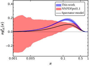
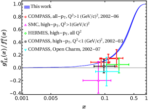
Figure 2: The gluon helicity pdf, $g_{1L}^{g}(x)$ (left panel) compared with the NNPDFpol1.1 Nocera et al. (2014) and the spectator model results Bacchetta et al. (2020) at $Q_{0}=2$ GeV. The right panel shows the comparison for the helicity asymmetry $g_{1L}^{g}(x)/f_{1}^{g}(x)$ from our calculation (blue band) with the experimental measurements. The direct measurements of COMPASS Ageev et al. (2006); Adolph et al. (2017), HERMES Airapetian et al. (2010) and SMC Adeva et al. (2004) are obtained in the leading order from high $p_{T}$ hadrons while open charm muon production at COMPASS  Adolph et al. (2013) are taken from next-to-leading order at different values of $x$.

In Fig. 2, we show our model predictions for the polarized gluon distribution $xg_{1L}^{g}(x)$ (left panel) and the gluon helicity asymmetry ratio $g^{g}_{1L}(x)/f_{1}^{g}(x)$ (right panel) at $Q_{0}=2$ GeV. The red band in the left panel of Fig. 2 represents the NNPDFpol1.1 results, which have large uncertainty in the entire range of $x$ and particularly in the small-$x$ region. The central line of NNPDFpol1.1 data is negative in the $x$ close to $0.001$ region, while in our model, the gluon helicity distribution is always positive. Overall, we find that our gluon helicity distribution in the entire region of $x$ except the domain $0.07<x<0.3$ is more or less consistent with the global analysis. Within the domain $0.07<x<0.3$, the distribution is going beyond the uncertainty band. As a result, we obtain the high value of gluon spin contribution in the small-$x$ region as shown in Table 3. The spin contribution for large-$x$ mainly comes from the quark sector and we can not expect much contribution from gluons. In Table 3, we list the dependence of the gluon helicity on the $x$ range and also compare them with the other model predictions of gluon helicity in certain ranges of $x$. We observe that the maximum contribution to the gluon helicity comes from the small-$x$ region. Compared to other model results, the gluon helicity contributions for different $x$ regions are found to be relatively larger in our model. The high gluon spin contribution has been reported in Refs. Joó et al. (2019); Kaur and Dahiya (2019). Meanwhile, in Ref. Bacchetta et al. (2020), the gluon spin contribution is relatively small, $s_{g}=0.159\pm 0.011$, which may be due to the fact that the unpolarized as well as helicity PDFs have been simultaneously fitted in that model. The latest lattice result of the gluon total angular momentum is reported to be $J_{g}=0.187(46)$ at the scale $2$ GeV Alexandrou et al. (2020).

Table 3: Comparison of the numerical values of the gluon spin contribution with the available data at $Q_{0}=2$ GeV.

Gluon helicity	Central Value	our predictions
$\Delta G=\int_{0.05}^{0.3}dx\Delta g(x)$	0.20    Adare et al. (2009)	$0.28_{-0.037}^{+0.047}$
$\Delta$G=$\int_{0.05}^{0.2}dx\Delta g(x)$	0.23(6) Nocera et al. (2014)	$0.22^{+0.033}_{-0.024}$
$\Delta$G=$\int_{0.05}^{1}dx\Delta g(x)$	0.19(6) de Florian et al. (2014)	$0.326^{+0.066}_{-0.050}$

In the right panel of Fig. 2, the gluon helicity asymmetry has been compared with available experimental data. From this comparison, we notice that our result for helicity asymmetry is in good agreement with the experimental measurements. In our model, the helicity asymmetry ratio is independent of the model parameters $a$ and $b$ and depends only on the spectator mass $M_{x}$, which satisfies the following model-independent QCD constraints Brodsky and Schmidt (1990); Brodsky et al. (1995) ,

$$\lim_{x\rightarrow 0}\frac{g_{1L}^{g}(x)}{f_{1}^{g}(x)}=0,\hskip 14.22636pt{\rm and}\hskip 14.22636pt\lim_{x\rightarrow 1}\frac{g_{1L}^{g}(x)}{f_{1}^{g}(x)}=1.$$ (23)

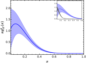
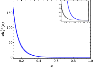
Figure 3: The gluon worm-gear, $xg_{1L}^{g}(x)$ (left) and the Boer-Mulders, $xh_{1}^{\perp g}(x)$ (right) collinear PDFs. The insets show a comparison of our results to those presented in Ref. Lyubovitskij and Schmidt (2021b) with dashed borders.

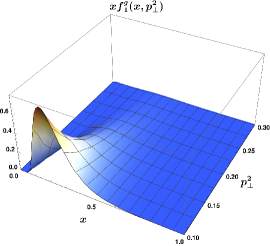
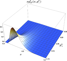
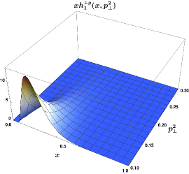
Figure 4: The TMDs for the gluon as functions of $x$ and ${\bf p}_{\perp}^{2}$. Upper panel: The unpolarized gluon TMD, $f_{1}^{g}(x,{\bf p}_{\perp}^{2})$ (left), The gluon helicity TMD, $g_{1L}^{g}(x,{\bf p}_{\perp}^{2})$ (right panel). Lower panel: The worm-gear TMD, $g_{1T}^{g}(x,{\bf p}_{\perp}^{2})$ (left) and the Boer-Mulders TMD, $h_{1}^{\perp g}(x,{\bf p}_{\perp}^{2})$ (right).

The uncertainty band in the helicity asymmetry ratio plot (Fig. 2) is created by including the errors in the spectator mass ($M_{x}=0.985^{+0.044}_{-0.045}$) in such a way that the maximum spin contribution should not go beyond the total proton spin and the lower cut-off for the spectator mass is $M_{x}\to M$.

In Fig. 3, we show $x$-weighted collinear PDFs of worm-gear $g_{1T}^{g}(x)$ and the Boer-Mulders $h_{1}^{\perp g}(x)$ TMDs as a function of $x$. There is no PDF corresponding to the collinear limit of the worm-gear and the Boer-Mulders TMDs. We have also shown their comparison with the results reported in Ref. Lyubovitskij and Schmidt (2021b) in the range $0<x<0.6$.

The three-dimensional distribution of the T-even TMDs, $f_{1}^{g}(x,{\bf p}_{\perp}^{2})$, $g_{1L}^{g}(x,{\bf p}_{\perp}^{2})$, $g_{1T}^{g}(x,{\bf p}_{\perp}^{2})$, and $h_{1}^{\perp g}(x,{\bf p}_{\perp}^{2})$ at the scale $Q_{0}=2$ GeV are shown in Fig. 4. All the T-even TMDs have their positive peaks around small $x$ and fall off very sharply with increasing ${\bf p}_{\perp}$. In Fig. 5, we present our model results for the T-even gluon TMDs as a function of ${\bf p}_{\perp}^{2}$ at $x=0.1$. These distributions are found to be slightly overestimated as compared to the results reported in Ref. Lyubovitskij and Schmidt (2021b), whereas the worm-gear TMD in Ref. Bacchetta et al. (2020) is shown to be negative. We also notice that our model results for T-even TMDs fall off very sharply with ${\bf p}_{\perp}^{2}$ as compared to the other theoretical predictions Lyubovitskij and Schmidt (2021b); Bacchetta et al. (2020); Kaur and Dahiya (2019).

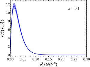
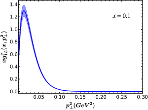
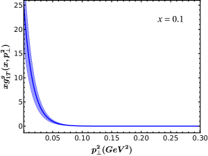
Figure 5: The T-even TMDs as a function of ${\bf p}_{\perp}^{2}$ for $x=0.1$. Upper panel: The unpolarized gluon TMD, $xf_{1}^{g}(x,{\bf p}_{\perp}^{2})$ (left), The helicity TMD, $xg_{1L}^{g}(x,{\bf p}_{\perp}^{2})$ (right). Lower panel: The worm-gear TMD, $g_{1T}^{g}(x,{\bf p}_{\perp}^{2})$ (left) and the Boer-Mulders TMD, $h_{1}^{\perp g}(x,{\bf p}_{\perp}^{2})$ (right), respectively.

The following gluon densities are also pertinent since they describe the two-dimensional ${\bf p}_{\perp}$-distributions of gluons at various $x$ for various combinations of their polarization and nucleon spin state. The unpolarized gluon density in an unpolarized nucleon is calculated as follows:

$$x\rho_{g}(x,p_{x},p_{y})=xf_{1}^{g}(x,{\bf p}_{\perp}^{2}),$$ (24)

which describes the probability density of finding the unpolarized gluons at given $x$ and ${\bf p}_{\perp}$. The “Boer-Mulders” density, which shows the probability density of finding the linearly polarized gluons with $x$ and ${\bf p}_{\perp}$ is given as,

$$x\rho^{\leftrightarrow}_{g}(x,p_{x},p_{y})=\frac{1}{2}\bigg{[}xf_{1}^{g}(x,{\bf p}_{\perp}^{2})+\frac{p_{x}^{2}-p_{y}^{2}}{2M^{2}}xh_{1}^{\perp g}(x,{\bf p}_{\perp}^{2})\bigg{]}.$$ (25)

Similarly, the “helicity density”, which describes the probability density of circularly polarized gluons at particular $x$ and ${\bf p}_{\perp}$ inside the longitudinally polarized proton is given as,

$$x\rho^{\circlearrowleft/+}_{g}(x,p_{x},p_{y})=xf_{1}^{g}(x,{\bf p}_{\perp}^{2})+xg_{1L}^{g}(x,{\bf p}_{\perp}^{2}).$$ (26)

Finally, the “worm-gear density”, which describes the probability density of circularly polarized gluons at given $x$ and ${\bf p}_{\perp}$ inside the transversely polarized proton is given as,

$$x\rho^{\circlearrowleft/\leftrightarrow}_{g}(x,p_{x},p_{y})=xf_{1}^{g}(x,{\bf p}_{\perp}^{2})-\frac{p_{x}}{M}xg_{1T}^{g}(x,{\bf p}_{\perp}^{2}).$$ (27)

The unpolarized, Eq. (24), and the helicity, Eq. (26), densities show that the ${\bf p}_{\perp}$ distributions are cylindrically symmetric around the longitudinal direction, as the proton (gluon) is unpolarized or longitudinally (circularly) polarized along to $P^{+}$. The Boer-Mulders density Eq. (25) is symmetric about the $p_{x}$ and $p_{y}$ axes because it describes unpolarized proton and linearly polarized gluons along the $p_{x}$ direction. The worm-gear density involves a transversely polarized proton along the $+p_{x}$ axes. Hence it is asymmetrically distributed in the same direction.

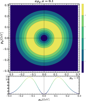
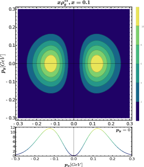
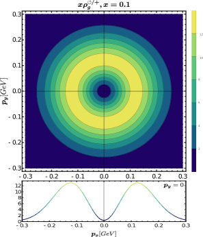
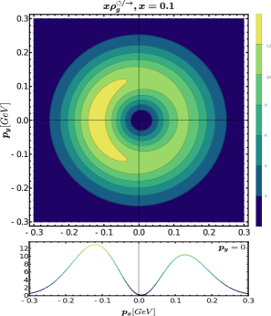
Figure 6: Upper panel: unpolarized gluon density (left), Boer-Mulders gluon density (right) for a virtually moving unpolarized nucleon. Lower panel: helicity gluon density (left) and worm-gear gluon density (right) for a polarized nucleon virtually moving towards the reader. 1D ancillary plots for each contour plot indicate the density at $p_{y}=0$. All densities are represented as a function of ${\bf p}_{\perp}\equiv(p_{x},p_{y})$ at a constant $x=0.1$.

In Fig. 6 we show the contour plots for the ${\bf p}_{\perp}$-distribution of the densities at $x=0.1$. The upper left panel shows the unpolarized density, $\rho_{g}$ which is cylindrically symmetric in the $p_{x}$ and $p_{y}$ directions followed by the ancillary 1D plots which represents the corresponding density at $p_{y}=0$. The upper right panel represents the BM density, $\rho^{\leftrightarrow}$ which shows a quadrupole structure. The lower left panel presents the gluon helicity density, $\rho^{\circlearrowleft/+}$ which is perfectly symmetric in the transverse plane because it describes a proton (gluon) longitudinally (circularly) polarized along the direction of motion pointing towards the reader. The lower right panel represents the worm-gear density, $\rho^{\circlearrowleft/\leftrightarrow}$ which is slightly asymmetric in $p_{x}$ at $x=0.1$ because the proton is transversely polarized along the $p_{x}$-direction. The color code identifies the size of the oscillation of each density along the $p_{x}$ and $p_{y}$ directions.

V.1 Relations between TMDs

The gluon TMDs are very sensitive to $x$. The TMDs and their relations among them could be separated into small and large $x$ regions. Depending upon the applicability of the model these relations can be checked only in certain ranges of $x$. The leading twist TMDs in this model also satisfy the inequality relations, which are valid in QCD and all models Lyubovitskij and Schmidt (2021b, a), e.g., positivity bound, which is the most known model-independent relation. According to which the unpolarized TMD $f_{1}^{g}(x,{\bf p}_{\perp}^{2})$ should be always positive and larger than the polarized one Mulders and Rodrigues (2001) i.e.,

$$f_{1}^{g}(x,{\bf p}_{\perp}^{2})>0,\hskip 14.22636ptf_{1}^{g}(x,{\bf p}_{\perp}^{2})\geq|g_{1L}^{g}(x,{\bf p}_{\perp}^{2})|.$$ (28)

and,

$$f_{1}^{g}(x,{\bf p}_{\perp}^{2})\geq\frac{|{\bf p}_{\perp}|}{M}|g_{1T}^{g}(x,{\bf p}_{\perp}^{2})|,\hskip 14.22636ptf_{1}^{g}(x,{\bf p}_{\perp}^{2})\geq\frac{|{\bf p}_{\perp}|^{2}}{2M^{2}}|h_{1}^{\perp g}(x,{\bf p}_{\perp}^{2})|.$$ (29)

Apart from these relations, there are several relations among TMDs themselves. The Mulders-Rodrigues relations for unpolarized and the polarised TMDs Mulders and Rodrigues (2001) are more stringent conditions than the above positivity bounds and are satisfied in our model:

$$\sqrt{[g_{1L}^{g}(x,{\bf p}_{\perp}^{2})]^{2}+\bigg{[}\frac{|{\bf p}_{\perp}|}{M}g_{1T}^{g}(x,{\bf p}_{\perp}^{2})\bigg{]}^{2}}\leq f_{1}^{g}(x,{\bf p}_{\perp}^{2}),$$

$$\sqrt{[g_{1L}^{g}(x,{\bf p}_{\perp}^{2})]^{2}+\bigg{[}\frac{{\bf p}_{\perp}^{2}}{2M^{2}}h_{1}^{\perp g}(x,{\bf p}_{\perp}^{2})\bigg{]}^{2}}\leq f_{1}^{g}(x,{\bf p}_{\perp}^{2}),$$

$$\sqrt{\bigg{[}\frac{|{\bf p}_{\perp}|}{M}g_{1T}^{g}(x,{\bf p}_{\perp}^{2})\bigg{]}^{2}+\bigg{[}\frac{{\bf p}_{\perp}^{2}}{2M^{2}}h_{1}^{\perp g}(x,{\bf p}_{\perp}^{2})\bigg{]}^{2}}\leq f_{1}^{g}(x,{\bf p}_{\perp}^{2}).$$ (30)

The positivity bounds Eqs. (28) and (29) can be derived as limiting cases of Eq.(V.1).

An interesting sum rule has been derived in Ref. Lyubovitskij and Schmidt (2021b) involving the T-even TMDs, by expressing them in terms of overlaps of LFWFs. This can be expressed as :

$$[f_{1}^{g}(x,{\bf p}_{\perp}^{2})]^{2}=[g_{1L}^{g}(x,{\bf p}_{\perp}^{2})]^{2}+\bigg{[}\frac{|{\bf p}_{\perp}|}{M}g_{1T}^{g}(x,{\bf p}_{\perp}^{2})\bigg{]}^{2}+\bigg{[}\frac{{\bf p}_{\perp}^{2}}{2M^{2}}h_{1}^{\perp g}(x,{\bf p}_{\perp}^{2})\bigg{]}^{2},$$ (31)

The above relation, Eq.(31), gives the connection between the square of an unpolarized TMD and a combination of squares of three polarised TMDs. In Fig. 7, we show the ratio of Boer-Mulders to unpolarized TMDs weighted by ${\bf p}_{\perp}^{2}/2M^{2}$ as a function of ${\bf p}_{\perp}$ for different values of the gluon longitudinal momentum fraction $x$. We notice that the positivity bound saturates only for the small $x$-values, for large $x$-values the positivity inequality is satisfied in the whole range of ${\bf p}_{\perp}$. Saturation of the positivity bound for gluon TMDs in a spectator model in the certain kinematical region has been reported in Ref. Kishore et al. (2022).

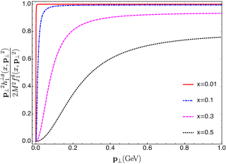
Figure 7: Positivity bound for different values of longitudinal momentum fraction $x$. The solid red curve shows the saturation of the positivity bound, whereas the other curves satisfy this constraint.

Note that all the relations listed above are independent of the parameters of our model.

VI Conclusion

We have proposed a light-front spectator model with the light-front wave functions modelled from the soft-wall holographic AdS/QCD prediction for two-body bound states. In this simple model, proton is assumed to consist of a struck gluon and a spin-1/2 spectator. We fixed our model parameters by fitting the unpolarized gluon PDF, $f_{1}^{g}(x)$ with the NNPDF3.0nlo global analysis. The helicity PDF and other T-even TMDs are calculated as predictions of the model and are shown to satisfy the positivity bound and have in good agreement with the available model predictions. The model is found to satisfy the constraints imposed by QCD including counting rules at small and large $x$. We have demonstrated that the gluon TMDs obey the model-independent Mulders-Rodrigues inequalities. We have also shown in this model that the superposition of the squares of all polarized T-even TMDs is equal to the square of the unpolarized TMD. We verified that this sum rule is also followed in similar models. It will be interesting to study the other proton properties like GPDs, T-odd TMDs, Wigner distributions, GTMDs, etc., and their scale evolutions in this model, and to compare with other model predictions, which can be helpful for the upcoming EICs.

References

- Meissner et al. (2007) S. Meissner, A. Metz, and K. Goeke, Phys. Rev. D 76, 034002 (2007), eprint hep-ph/0703176.
- Jakob et al. (1997) R. Jakob, P. J. Mulders, and J. Rodrigues, Nucl. Phys. A 626, 937 (1997), eprint hep-ph/9704335.
- Brodsky et al. (2002) S. J. Brodsky, D. S. Hwang, and I. Schmidt, Phys. Lett. B 530, 99 (2002), eprint hep-ph/0201296.
- Bacchetta et al. (2008) A. Bacchetta, F. Conti, and M. Radici, Phys. Rev. D 78, 074010 (2008), eprint 0807.0323.
- Pasquini et al. (2008) B. Pasquini, S. Cazzaniga, and S. Boffi, Phys. Rev. D 78, 034025 (2008), eprint 0806.2298.
- Maji and Chakrabarti (2017) T. Maji and D. Chakrabarti, Phys. Rev. D 95, 074009 (2017), eprint 1702.04557.
- Gurjar et al. (2021) B. Gurjar, D. Chakrabarti, P. Choudhary, A. Mukherjee, and P. Talukdar, Phys. Rev. D 104, 076028 (2021), eprint 2107.02216.
- Gurjar et al. (2022) B. Gurjar, D. Chakrabarti, and C. Mondal, Phys. Rev. D 106, 114027 (2022), eprint 2207.11527.
- Lorce and Pasquini (2011) C. Lorce and B. Pasquini, Phys. Rev. D 84, 034039 (2011), eprint 1104.5651.
- Ji et al. (1997) X.-D. Ji, W. Melnitchouk, and X. Song, Phys. Rev. D 56, 5511 (1997), eprint hep-ph/9702379.
- Scopetta and Vento (2003) S. Scopetta and V. Vento, Eur. Phys. J. A 16, 527 (2003), eprint hep-ph/0201265.
- Boffi et al. (2003) S. Boffi, B. Pasquini, and M. Traini, Nucl. Phys. B 649, 243 (2003), eprint hep-ph/0207340.
- Boffi et al. (2004) S. Boffi, B. Pasquini, and M. Traini, Nucl. Phys. B 680, 147 (2004), eprint hep-ph/0311016.
- Vega et al. (2011) A. Vega, I. Schmidt, T. Gutsche, and V. E. Lyubovitskij, Phys. Rev. D 83, 036001 (2011), eprint 1010.2815.
- Chakrabarti and Mondal (2013) D. Chakrabarti and C. Mondal, Phys. Rev. D 88, 073006 (2013), eprint 1307.5128.
- Mondal and Chakrabarti (2015) C. Mondal and D. Chakrabarti, Eur. Phys. J. C 75, 261 (2015), eprint 1501.05489.
- Chakrabarti and Mondal (2015) D. Chakrabarti and C. Mondal, Phys. Rev. D 92, 074012 (2015), eprint 1509.00598.
- Xu et al. (2021) S. Xu, C. Mondal, J. Lan, X. Zhao, Y. Li, and J. P. Vary (BLFQ), Phys. Rev. D 104, 094036 (2021), eprint 2108.03909.
- Kriesten et al. (2022) B. Kriesten, P. Velie, E. Yeats, F. Y. Lopez, and S. Liuti, Phys. Rev. D 105, 056022 (2022), eprint 2101.01826.
- Chakrabarti et al. (2016) D. Chakrabarti, T. Maji, C. Mondal, and A. Mukherjee, Eur. Phys. J. C 76, 409 (2016), eprint 1601.03217.
- Meissner et al. (2008) S. Meissner, A. Metz, M. Schlegel, and K. Goeke, JHEP 08, 038 (2008), eprint 0805.3165.
- Meissner et al. (2009) S. Meissner, A. Metz, and M. Schlegel, JHEP 08, 056 (2009), eprint 0906.5323.
- Burkert et al. (2023) V. D. Burkert, L. Elouadrhiri, F. X. Girod, C. Lorce, P. Schweitzer, and P. E. Shanahan (2023), eprint 2303.08347.
- Ji et al. (2021) X. Ji, F. Yuan, and Y. Zhao, Nature Rev. Phys. 3, 27 (2021), eprint 2009.01291.
- Jaffe and Manohar (1990) R. L. Jaffe and A. Manohar, Nucl. Phys. B 337, 509 (1990).
- Ji (1997) X. Ji, Phys. Rev. Lett. 78, 610 (1997).
- Leader (2022) E. Leader, Phys. Rev. D 105, 036005 (2022), eprint 2108.07730.
- Liu and Lorcé (2016) K.-F. Liu and C. Lorcé, Eur. Phys. J. A 52, 160 (2016), eprint 1508.00911.
- Xie and Lu (2022) X. Xie and Z. Lu (2022), eprint 2210.16532.
- Khan et al. (2021) T. Khan et al. (HadStruc), Phys. Rev. D 104, 094516 (2021), eprint 2107.08960.
- Yang et al. (2017) Y.-B. Yang, R. S. Sufian, A. Alexandru, T. Draper, M. J. Glatzmaier, K.-F. Liu, and Y. Zhao, Phys. Rev. Lett. 118, 102001 (2017), eprint 1609.05937.
- Delmar et al. (2022) J. Delmar, C. Alexandrou, K. Cichy, M. Constantinou, and K. Hadjiyiannakou (2022), eprint 2212.11399.
- Sufian et al. (2021) R. S. Sufian, T. Liu, and A. Paul, Phys. Rev. D 103, 036007 (2021), eprint 2012.01532.
- Brodsky et al. (2001) S. J. Brodsky, D. S. Hwang, B.-Q. Ma, and I. Schmidt, Nucl. Phys. B 593, 311 (2001), eprint hep-th/0003082.
- Dosch et al. (2022) H. G. Dosch, G. F. de Téramond, T. Liu, R. S. Sufian, S. J. Brodsky, and A. Deur (HLFHS), Phys. Rev. D 105, 034029 (2022), eprint 2201.09813.
- Hou et al. (2021) T.-J. Hou et al., Phys. Rev. D 103, 014013 (2021), eprint 1912.10053.
- Ball et al. (2017) R. D. Ball et al. (NNPDF), Eur. Phys. J. C 77, 663 (2017), eprint 1706.00428.
- Freese et al. (2021) A. Freese, I. C. Cloët, and P. C. Tandy, Phys. Lett. B 823, 136719 (2021), eprint 2103.05839.
- de Florian et al. (2014) D. de Florian, R. Sassot, M. Stratmann, and W. Vogelsang, Phys. Rev. Lett. 113, 012001 (2014), eprint 1404.4293.
- Ashman et al. (1988) J. Ashman et al. (European Muon), Phys. Lett. B 206, 364 (1988).
- Ashman et al. (1989) J. Ashman et al. (European Muon), Nucl. Phys. B 328, 1 (1989).
- de Florian et al. (2009) D. de Florian, R. Sassot, M. Stratmann, and W. Vogelsang, Phys. Rev. D 80, 034030 (2009), eprint 0904.3821.
- Nocera et al. (2014) E. R. Nocera, R. D. Ball, S. Forte, G. Ridolfi, and J. Rojo (NNPDF), Nucl. Phys. B 887, 276 (2014), eprint 1406.5539.
- Ethier et al. (2017) J. J. Ethier, N. Sato, and W. Melnitchouk, Phys. Rev. Lett. 119, 132001 (2017), eprint 1705.05889.
- Adare et al. (2014) A. Adare et al. (PHENIX), Phys. Rev. D 90, 012007 (2014), eprint 1402.6296.
- Adare et al. (2009) A. Adare et al. (PHENIX), Phys. Rev. Lett. 103, 012003 (2009), eprint 0810.0694.
- Adolph et al. (2016) C. Adolph et al. (COMPASS), Phys. Lett. B 753, 18 (2016), eprint 1503.08935.
- Xu et al. (2022) S. Xu, C. Mondal, X. Zhao, Y. Li, and J. P. Vary (2022), eprint 2209.08584.
- Gurjar et al. (2023) B. Gurjar, C. Mondal, and D. Chakrabarti, Phys. Rev. D 107, 054013 (2023), eprint 2209.14285.
- Khan et al. (2022) T. Khan, T. Liu, and R. S. Sufian (2022), eprint 2211.15587.
- Egerer et al. (2022) C. Egerer et al. (HadStruc), Phys. Rev. D 106, 094511 (2022), eprint 2207.08733.
- Gehrmann and Stirling (1996) T. Gehrmann and W. J. Stirling, Phys. Rev. D 53, 6100 (1996), eprint hep-ph/9512406.
- Gluck et al. (2001) M. Gluck, E. Reya, M. Stratmann, and W. Vogelsang, Phys. Rev. D 63, 094005 (2001), eprint hep-ph/0011215.
- Blumlein and Bottcher (2002) J. Blumlein and H. Bottcher, Nucl. Phys. B 636, 225 (2002), eprint hep-ph/0203155.
- Accardi et al. (2016) A. Accardi et al., Eur. Phys. J. A 52, 268 (2016), eprint 1212.1701.
- Abdul Khalek et al. (2022) R. Abdul Khalek et al., Nucl. Phys. A 1026, 122447 (2022), eprint 2103.05419.
- Anderle et al. (2021) D. P. Anderle et al., Front. Phys. (Beijing) 16, 64701 (2021), eprint 2102.09222.
- Ji (1995a) X.-D. Ji, Phys. Rev. Lett. 74, 1071 (1995a), eprint hep-ph/9410274.
- Ji (1995b) X.-D. Ji, Phys. Rev. D 52, 271 (1995b), eprint hep-ph/9502213.
- Rodini et al. (2020) S. Rodini, A. Metz, and B. Pasquini, JHEP 09, 067 (2020), eprint 2004.03704.
- Metz et al. (2020) A. Metz, B. Pasquini, and S. Rodini, Phys. Rev. D 102, 114042 (2020), eprint 2006.11171.
- Lorcé et al. (2021) C. Lorcé, A. Metz, B. Pasquini, and S. Rodini, JHEP 11, 121 (2021), eprint 2109.11785.
- D’Alesio et al. (2019) U. D’Alesio, C. Flore, F. Murgia, C. Pisano, and P. Taels, Phys. Rev. D 99, 036013 (2019), eprint 1811.02970.
- Mulders and Rodrigues (2001) P. J. Mulders and J. Rodrigues, Phys. Rev. D 63, 094021 (2001), eprint hep-ph/0009343.
- Boer et al. (2016) D. Boer, M. G. Echevarria, P. Mulders, and J. Zhou, Phys. Rev. Lett. 116, 122001 (2016), eprint 1511.03485.
- Lyubovitskij and Schmidt (2021a) V. E. Lyubovitskij and I. Schmidt, Phys. Rev. D 104, 014001 (2021a), eprint 2105.07842.
- Bacchetta et al. (2020) A. Bacchetta, F. G. Celiberto, M. Radici, and P. Taels, Eur. Phys. J. C 80, 733 (2020), eprint 2005.02288.
- Lu and Ma (2016) Z. Lu and B.-Q. Ma, Phys. Rev. D 94, 094022 (2016), eprint 1611.00125.
- Petreska (2018) E. Petreska, Int. J. Mod. Phys. E 27, 1830003 (2018), eprint 1804.04981.
- Altinoluk et al. (2019) T. Altinoluk, R. Boussarie, C. Marquet, and P. Taels, JHEP 07, 079 (2019), eprint 1810.11273.
- Altinoluk et al. (2020) T. Altinoluk, R. Boussarie, C. Marquet, and P. Taels, JHEP 07, 143 (2020), eprint 2001.00765.
- Zhou (2019) J. Zhou, Phys. Rev. D 99, 054026 (2019), eprint 1807.00506.
- Lyubovitskij and Schmidt (2021b) V. E. Lyubovitskij and I. Schmidt, Phys. Rev. D 103, 094017 (2021b), eprint 2012.01334.
- Tan and Lu (2023) C. Tan and Z. Lu (2023), eprint 2301.09081.
- Brodsky and Schmidt (1990) S. J. Brodsky and I. A. Schmidt, Phys. Lett. B 234, 144 (1990).
- Brodsky et al. (1995) S. J. Brodsky, M. Burkardt, and I. Schmidt, Nucl. Phys. B 441, 197 (1995), eprint hep-ph/9401328.
- Brodsky et al. (2015) S. J. Brodsky, G. F. de Teramond, H. G. Dosch, and J. Erlich, Phys. Rept. 584, 1 (2015), eprint 1407.8131.
- Gutsche et al. (2014) T. Gutsche, V. E. Lyubovitskij, I. Schmidt, and A. Vega, Phys. Rev. D 89, 054033 (2014), [Erratum: Phys.Rev.D 92, 019902 (2015)], eprint 1306.0366.
- Maji and Chakrabarti (2016) T. Maji and D. Chakrabarti, Phys. Rev. D 94, 094020 (2016), eprint 1608.07776.
- More et al. (2018) J. More, A. Mukherjee, and S. Nair, Eur. Phys. J. C 78, 389 (2018), eprint 1709.00943.
- Ball et al. (2018) R. D. Ball, V. Bertone, M. Bonvini, S. Marzani, J. Rojo, and L. Rottoli, Eur. Phys. J. C 78, 321 (2018), eprint 1710.05935.
- Alexandrou et al. (2020) C. Alexandrou, S. Bacchio, M. Constantinou, J. Finkenrath, K. Hadjiyiannakou, K. Jansen, G. Koutsou, H. Panagopoulos, and G. Spanoudes, Phys. Rev. D 101, 094513 (2020), eprint 2003.08486.
- Kaur and Dahiya (2019) N. Kaur and H. Dahiya, DAE Symp. Nucl. Phys. 64, 641 (2019).
- Ageev et al. (2006) E. S. Ageev et al. (COMPASS), Phys. Lett. B 633, 25 (2006), eprint hep-ex/0511028.
- Adolph et al. (2017) C. Adolph et al. (COMPASS), Eur. Phys. J. C 77, 209 (2017), eprint 1512.05053.
- Airapetian et al. (2010) A. Airapetian et al. (HERMES), JHEP 08, 130 (2010), eprint 1002.3921.
- Adeva et al. (2004) B. Adeva et al. (Spin Muon (SMC)), Phys. Rev. D 70, 012002 (2004), eprint hep-ex/0402010.
- Adolph et al. (2013) C. Adolph et al. (COMPASS), Phys. Rev. D 87, 052018 (2013), eprint 1211.6849.
- Joó et al. (2019) B. Joó, J. Karpie, K. Orginos, A. V. Radyushkin, D. G. Richards, R. S. Sufian, and S. Zafeiropoulos, Phys. Rev. D 100, 114512 (2019), eprint 1909.08517.
- Kishore et al. (2022) R. Kishore, A. Mukherjee, A. Pawar, and M. Siddiqah, Phys. Rev. D 106, 034009 (2022), eprint 2203.13516.