$\mathbb{Z}_{2}$-Nontrivial Moiré Minibands and Interaction-Driven Quantum Anomalous Hall Insulators in Topological Insulator Based Moiré Heterostructures

Abstract

We studied electronic band structure and topological property of a topological insulator thin film under a moiré superlattice potential to search for two-dimensional (2D) $\mathbb{Z}_{2}$ non-trivial isolated mini-bands. To model this system, we assume the Fermi energy inside the bulk band gap and thus consider an effective model Hamiltonian with only two surface states that are located at the top and bottom surfaces and strongly hybridized with each other. The moiré potential is generated by another layer of 2D insulating materials on top of topological insulator films. In this model, the lowest conduction (highest valence) mini-bands can be $\mathbb{Z}_{2}$ non-trivial when the minima (maxima) of the moiré potential approximately forms a hexagonal lattice with six-fold rotation symmetry. For the nontrivial conduction mini-band cases, the two lowest Kramers’ pairs of conduction mini-bands both have nontrivial $\mathbb{Z}_{2}$ invariant in presence of inversion, while applying external gate voltages to break inversion leads to only the lowest Kramers’ pair of mini-bands to be topologically non-trivial. The Coulomb interaction can drive the lowest conduction Kramers’ mini-bands into the quantum anomalous Hall state when they are half-filled, which is further stabilized by breaking inversion symmetry. We propose the monolayer Sb₂ on top of Sb₂Te₃ thin films to realize our model based on results from the first principles calculations.

Introduction - Recent research interests have focused on the moiré superlattice in 2D Van der Waals heterostructures, including grapheneBistritzer and MacDonald (2011); Cao et al. (2018a, b); Sharpe et al. (2019); Yankowitz et al. (2019); Serlin et al. (2020); Lu et al. (2019); Kennes et al. (2021) and transition metal dichalcogenide (TMD) multilayersZhang et al. (2017); Mak and Shan (2022); Wu et al. (2018); Regan et al. (2020); Tang et al. (2020); Alexeev et al. (2019); Jin et al. (2019); Seyler et al. (2019); Tran et al. (2019) , due to the strong correlation effect in the presence of flat bands. The flat bands formed by low-energy gapless Dirac fermions in magic angle twisted bilayer graphene typically have a bandwidth $\sim 5$ meV, much smaller than the band gap $25\sim 35$ meV that separates flat bands from higher energy bands and the Coulomb interaction of order $30$ meVCao et al. (2018b, a). In contrast, the flat bands in TMD moiré heterostructures are formed by electrons with parabolic dispersion and have a typical bandwidth $\sim 10$ meV, separated by a comparable gap from other energy bands, and a huge on-site Coulomb interaction $\sim 100$ meVMak and Shan (2022); Devakul et al. (2021); Wu et al. (2018). Besides the above materials, moiré superlattice has also been found in another family of van der Waals heterostructure consisting of topological insulators (TIs) Chang et al. (2015a); Salvato et al. (2022); Schouteden et al. (2016); Yin et al. (2022); Song et al. (2010); Wang et al. (2012); Liu et al. (2014); Xu et al. (2015); Vargas et al. (2017); Liu et al. . These TI-based moiré heterostructures show different features. TIs have the anomalous gapless surface bands that connect the bulk conduction and valence bands due to non-trivial bulk topology. The spin splitting of surface bands has a typical energy scale of hundreds meV due to the strong spin-orbit coupling (SOC). Previous studiesCano et al. (2021); Dunbrack and Cano (2022); Wang et al. (2021) show that a single surface state remains gapless upon the moiré superlattice potential, leading to satellite Dirac cones and van Hove singularities, instead of isolated flat bands. Furthermore, the moiré superlattice in magnetic TI materials, e.g. MnBi₂Te₄, is predicted to host Chern insulator phaseLian et al. (2020).

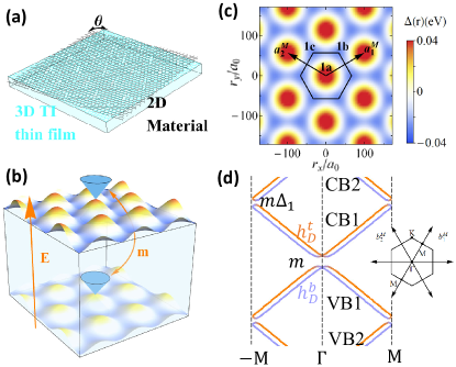
Figure 1: (a) A schematic figure for the twisted 2D materials (black) on top of a topological insulator thin film (cyan). (b) Schematic illustration of the moiré potentials from twisted 2D materials on the top and bottom surface of a TI thin film. The blue Dirac cones represent the top and bottom surface states coupled by $m$. An out-of-plane external electrical field $E$ creates the potential $V_{0}$. (c) The moiré potential $\Delta({\textbf{{r}}})$ with $\phi=0$. $a_{1}^{M},a_{2}^{M}$ are primitive vectors for a moiré unit cell. $1a,1b,1c$ are Wyckoff positions under the point group $C_{3v}$. (d) Schematic view of the spectrum. The orange (blue) lines are top (bottom) surface Dirac cones at $\Gamma,b_{1}^{\text{M}}$. Inset is the moiré BZ with the first shell moiré reciprocal lattice vectors.

In this work, we studied a model of the TI thin film (e.g. (Bi,Sb)₂Te₃ film) with the moiré superlattice potential (See Fig. 1). Different from a bulk TI, a strong hybridization between two surface states is expected for the TI thin film. The hybridization between two surface states can create isolated minibands that possess non-trivial $\mathbb{Z}_{2}$ topological invariant, denoted by $\nu$ below, in the low-energy moiré spectrum in a wide parameter space, particularly when the moiré potential approximately has six-fold rotation symmetry. In the presence of inversion symmetry, an emergent chiral symmetry in the low energy sector of surface states gives rise to $\nu_{\text{CB1}}+\nu_{\text{VB1}}=1$ for the lowest Kramers’ pair of conduction mini-bands, denoted as CB1, and the highest Kramers’ pair of valence minibands, denoted as VB1, in Fig. 1(d). We find $\nu_{\text{CB1}}=1,\nu_{\text{VB1}}=0$ ($\nu_{\text{CB1}}=0,\nu_{\text{VB1}}=1$) when the minima (maxima) of the moiré potential approximately form a hexagonal lattice. In the case of non-trivial CB1 ($\nu_{\text{CB1}}=1,\nu_{\text{VB1}}=0$), the lowest two Kramers’ pairs of conduction mini-bands (CB1 and CB2 in Fig. 1(d)) together can be adiabatically connected to the Kane-Mele modelKane and Mele (2005) when increasing quadratic terms, and thus CB2 is also topologically non-trivial, $\nu_{CB2}=1$. An asymmetric potential between two surface states can be generated by external gate voltages to break inversion but preserve six-fold rotation and generally induce the gap closing between different conduction mini-bands, leading to nodal phases. In the parameter regions where the conduction mini-bands are gapped from other mini-bands (parameter regions I, II, III in Fig. 2), the CB1 is always topologically non-trivial, $\nu_{CB1}=1$. We further study the influence of the Coulomb interaction via Hartree-Fock mean field theory when the CB1 carries $\nu_{CB1}=1$ and is half filled, and find that the quantum anomalous Hall (QAH) state competes with a trivial insulator state in region I of Fig. 2(c) and it can be robustly energetically favored by the asymmetric potential in region II. Finally, we propose a possible experimental realization of the TI-based moiré heterostructure consisting of a monolayer Sb₂ layer on top of Sb₂Te₃ thin films based on results from the first principles calculations.

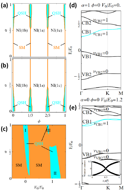
Figure 2: (a)(b) The topological phase diagrams of the lowest conduction bands CB1 for different moiré potentials with $V_{0}/E_{0}=0$ for (a) and $V_{0}/E_{0}=1.2$ for (b). (c) The phase diagram for different uniform asymmetrical potentials with $\phi=0$. Regions I, II and III are three parameter regimes with $\nu_{CB1}=1$ for CB1. (d)(e) Example spectra with nontrivial CB1 in the regions I and II, respectively. The spectrum in (d) has both TR and inversion, and is thus doubly degenerate. The inset of (e) is the Wannier center flow for CB1.

Model Hamiltonian - We show a schematic of a hetero-structure consisting of TI thin films and another 2D material (e.g. 2D Sb thin films) in Fig. 1(a) and (b), and the moiré potential induced by the 2D material can affect both the top and bottom surface states with different strength. We assume the Fermi energy is within the bulk gap of TI thin film, and thus model this system with the Hamiltonian

$$\begin{split}&H_{0}({\textbf{{r}}})=H^{\text{TI}}+H^{\text{M}}({\textbf{{r}}}),\\ &H^{\text{TI}}=v\tau_{z}(-i\partial_{y}s_{x}+i\partial_{x}s_{y})+m\tau_{x}s_{0},\\ &H^{\text{M}}({\textbf{{r}}})=\frac{1+\alpha}{2}\Delta({\textbf{{r}}})\tau_{0}s_{0}+\frac{1-\alpha}{2}\Delta({\textbf{{r}}})\tau_{z}s_{0}+V_{0}\tau_{z}s_{0}.\end{split}$$ (1)

$H^{\text{TI}}$ denotes two surface states of a TI thin film with the inter-surface hybridization $m=m_{0}+m_{2}(-\partial_{x}^{2}-\partial_{y}^{2})$, and $h^{t/b}_{D}({\textbf{{r}}})=\pm v(-i\partial_{y}s_{x}+i\partial_{x}s_{y})$ is the top/bottom surface Dirac HamiltonianYu et al. (2010). $s_{0,x,y,z}(\tau_{0,x,y,z})$ are the identity and Pauli matrices for spin (surfaces) and $v$ is the Fermi velocity. $H^{\text{M}}$ denotes the potential term, in which the $V_{0}$ term is the uniform asymmetric potential between two surfaces by gate voltages, the $\Delta({\textbf{{r}}})$ term is the moiré potential, and the $\alpha$ parameter ($0\leq\alpha\leq 1$) represents the asymmetry between top and bottom surfaces. $\Delta({\textbf{{r}}})$ is real, spin-independentCano et al. (2021), and assumed to possess the $C_{3v}$ symmetry coinciding with the atomic crystal symmetry of TI thin films. With the basis of the Hamiltonian, the corresponding symmetry operators are $C_{3z}=\exp(-i\pi\tau_{0}s_{z}/3)$ for three-fold rotation, $\mathcal{M}_{y}=\tau_{0}s_{y}$ for y-directional mirror, and $\mathcal{T}=i\tau_{0}s_{y}\mathcal{K}$ with $\mathcal{K}$ as complex conjugate for time-reversal. The moiré superlattice potential can be expanded as

$$\Delta({\textbf{{r}}})=\sum_{{\textbf{{G}}}}\Delta_{{\textbf{{G}}}}e^{i{\textbf{{G}}}\cdot{\textbf{{r}}}},$$ (2)

where ${{\textbf{{G}}}}=n_{1}{{\textbf{{b}}}}_{1}^{\text{M}}+n_{2}{{\textbf{{b}}}}_{2}^{\text{M}}$ is the moiré reciprocal lattice vectors with ${{\textbf{{b}}}}_{1}^{\text{M}}=\frac{4\pi}{\sqrt{3}|{{\textbf{{a}}}}_{1}^{\text{M}}|}(1/2,\sqrt{3}/2),{{\textbf{{b}}}}_{2}^{\text{M}}=\frac{4\pi}{\sqrt{3}|{{\textbf{{a}}}}_{1}^{\text{M}}|}(-1/2,\sqrt{3}/2)$ and $n_{1,2}$ as integers. ${{\textbf{{a}}}}_{1,2}^{\text{M}}$ are the primitive vectors for moiré superlattice (see Fig. 1(c)). The uniform part $\Delta_{{\textbf{{G}}}=0}$ can be absorbed into the chemical potential $\mu$ and the asymmetric potential $V_{0}$. To the lowest order, we only keep the first shell reciprocal lattice vectors $\pm{{\textbf{{b}}}}_{1}^{\text{M}},\pm{{\textbf{{b}}}}_{2}^{\text{M}},\pm({{\textbf{{b}}}}_{1}^{\text{M}}-{{\textbf{{b}}}}_{2}^{\text{M}})$ , as shown in Fig. 1(d). The values of $\Delta_{{\textbf{{G}}}}$ for different Gs are connected by three-fold rotation $C_{3z}$ and $\mathcal{T}$, so there is only one independent complex parameter, chosen to be $\Delta_{{\textbf{{b}}}_{1}^{\text{M}}}=\Delta_{1}e^{i2\pi\phi}$, where $\Delta_{1}$ is real and $\phi$ is the phase that tunes the relative strengths of potentials at three Wyckoff positions $1a,1b,1c$ in one moiré unit cell. Fig. 1(c) shows the moiré potential at $\phi=0$ with an additional six-fold rotation symmetry $C_{6z}=\exp(-i\pi\tau_{0}s_{z}/6)$, and the corresponding potential minima form the multiplicity-2 Wyckoff positions of the hexagonal lattice. The parameters used in our calculations below are $|{\textbf{{a}}}_{1}^{\text{M}}|=28$nm, $E_{0}=v|{\textbf{{b}}}_{1}^{\text{M}}|=38.5$ meV,Liu et al. (2010a) $m_{0}=0.4E_{0},~{}\Delta_{1}=0.24E_{0}$. The $m_{2}$ term and other quadratic terms are negligible for the low energy mini-bands in realistic materials as the relevant energy scale is around $1$ meV with a typical moiré momentum $10^{-2}\text{\AA}^{-1}$, much smaller than other terms in $H^{\text{TI}}$. But we still keep this term in low energy Hamiltonian as it plays an important role for connecting this model to the Kane-Mele model discussed below.

$\mathbb{Z}_{2}$ nontrivial moiré minibands - We first illustrate the crucial role of inter-surface hybridization in inducing isolated moiré minibands in TI thin films through the schematic view of the spectrum in Fig. 1(d). For a single Dirac surface state, it is knownCano et al. (2021); Mora et al. (2019); Wang et al. (2021) that moiré potential can fold the Dirac dispersion and the band touchings at the TR-invariant momenta, e.g. $\Gamma$ and $M$, in the moiré BZ remain gapless due to the Kramers’ theorem of TR symmetry. This leads to satellite Dirac cones, but prevents the formation of gaps and hence of isolated moiré minibands. For TI thin films, the inter-surface hybridization $m$ can directly result in a gap at $\Gamma$ while its combined effect with the moiré potential $\Delta({\textbf{{r}}})$ can lead to a gap (proportional to $m\Delta_{1}$) at $M$ (Fig. 1(d)). The gap openings at both $\Gamma$ and $M$ lead to the isolated moiré minibands, as demonstrated in Fig. 2(d) and (e) for the moiré spectrum of the model Hamiltonian (1) with different sets of parameters.

We are interested in the possibility of realizing ${\mathbb{Z}}_{2}$-nontrivial moiré mini-bands, particularly the low-energy Kramers’ pairs of conduction (valence) mini-bands, labelled by CB1, CB2 (VB1, VB2) in Fig. 2(d) and (e). For the parameters in Fig. 2(d), CB1 and CB2 are topologically non-trivial while VB1 and VB2 are trivial ($\nu_{\text{CB1}}=\nu_{\text{CB2}}=1$, $\nu_{\text{VB1}}=\nu_{\text{VB2}}=0$). For the parameters in Fig. 2(e), only CB1 is non-trivial while other mini-bands are trivial ($\nu_{\text{CB1}}=1,\nu_{\text{CB2}}=\nu_{\text{VB1}}=\nu_{\text{VB2}}=0$). Fig. 2(a) and (b) show the ${\mathbb{Z}}_{2}$-invariant $\nu_{\text{CB1}}$ for CB1 as a function of $\alpha$ and $\phi$ for a fixed $V_{0}/E_{0}=0$ and $1.2$, respectively. The blue regions correspond to $\nu_{\text{CB1}}=1$ while the white regions to $\nu_{\text{CB1}}=0$, and these two regions are separated by metallic lines (orange color). For both $V_{0}$ values, the $\nu_{\text{CB1}}=1$ blue regions appear around $\phi=0,1/3,2/3$. At these $\phi$ values, there is an additional $C_{6z}$ rotation symmetry, leading to a hexagonal lattice with the $C_{6v}$ group. Fig. 2(c) shows $\nu_{\text{CB1}}$ at $\phi=0$ as a function of $\alpha$ and $V_{0}$, and we find three different parameter regions I, II, III with $\nu_{\text{CB1}}=1$. These topologically non-trivial regions are separated by semi-metal phases that have band touchings between CB1 and CB2. $\nu_{\text{CB1}}$ for other $\phi$ is discussed in SM Sec.I.B and normal insulator phases are discussed in SM Sec.I.D.

The region I can be adiabatically connected to the parameter set $\alpha=1,~{}V_{0}/E_{0}=0$ with the band dispersion shown in Fig. 2(d), where the inversion symmetry $\mathcal{I}=\tau_{x}s_{0}$ and the horizontal mirror symmetry $\mathcal{M}_{z}=-i\tau_{x}s_{z}$ are present ($D_{6h}$ group). From the Fu-Kane parity criterionFu and Kane (2007), the $\mathbb{Z}_{2}$-invariant $\nu$ can be determined by $(-1)^{\nu}=\prod_{i}\lambda_{\Gamma_{i}}$ and $\lambda_{\Gamma_{i}}$ is the parity of eigen-states at the TR invariant momenta $\Gamma_{i=1,...,4}$. In 2D moiré BZ, they are corresponding to one $\Gamma$ point and three $M$ points, their values can be derived analytically in the weak $\Delta_{1}$ limit (See SM Sec. I.A). The four eigen-states of $H^{\text{TI}}$ are denoted as $|\psi^{\text{TI}}_{I,m_{z}}({\textbf{{k}}})\rangle$ with the gauge choice to satisfy $\mathcal{I}|\psi^{\text{TI}}_{I,m_{z}}({\textbf{{k}}})\rangle=I|\psi^{\text{TI}}_{I,m_{z}}(-{\textbf{{k}}})\rangle$ and $\mathcal{M}_{z}|\psi^{\text{TI}}_{I,m_{z}}({\textbf{{k}}})\rangle=m_{z}|\psi^{\text{TI}}_{I,m_{z}}({\textbf{{k}}})\rangle$, where $I=\pm$ and $m_{z}=\pm i$. The eigen-energies for $|\psi^{\text{TI}}_{I,m_{z}}({\textbf{{k}}})\rangle$ is $E^{\text{TI}}_{I,m_{z}}({\textbf{{k}}})=\text{sgn}(m)I\sqrt{m^{2}+v^{2}k^{2}}$ and two opposite mirror-eigen-value states $|\psi^{\text{TI}}_{I,m_{z}=\pm i}({\textbf{{k}}})\rangle$ are degenerate. At $\Gamma$, $|\psi^{\text{TI}}_{+,m_{z}}(\Gamma)\rangle$ and $|\psi^{\text{TI}}_{-,m_{z}}(\Gamma)\rangle$ are just the bonding and anti-bonding states formed by the top and bottom surface states, respectively. As the eigen-energies depend on the sign of $\text{sgn}(m)I$, the eigen-state of CB1 is $|\psi_{\text{CB1},m_{z}}(\Gamma)\rangle=|\psi^{\text{TI}}_{+\text{sgn}(m),m_{z}}(\Gamma)\rangle$ with the energy $E_{\text{CB1},m_{z}}(\Gamma)=|m|$ and parity $\lambda^{\text{CB1}}_{\Gamma}=\text{sgn}(m)$, while the eigen-state of VB1 is $|\psi_{\text{VB1},m_{z}}(\Gamma)\rangle=|\psi^{\text{TI}}_{-\text{sgn}(m),m_{z}}(\Gamma)\rangle$ with the energy $E_{\text{VB1},m_{z}}(\Gamma)=-|m|$ and parity $\lambda^{\text{VB1}}_{\Gamma}=-\text{sgn}(m)$, so we get $\lambda^{\text{VB1}}_{\Gamma}=-\lambda^{\text{CB1}}_{\Gamma}$. At M, the potential term $\Delta_{1}$ that can be treated as perturbation couples the states $|\psi^{\text{TI}}_{I,m_{z}}({\textbf{{M}}})\rangle$ and $|\psi^{\text{TI}}_{I,m_{z}}(-{\textbf{{M}}})\rangle$. Based on the degenerate perturbation theory, the eigen-state of CB1 is $|\psi_{\text{CB1},m_{z}}({\textbf{{M}}})\rangle=(|\psi^{\text{TI}}_{+\text{sgn}(m),m_{z}}({\textbf{{M}}})\rangle-\text{sgn}(\Delta_{1})|\psi^{\text{TI}}_{+\text{sgn}(m),m_{z}}(-{\textbf{{M}}})\rangle)/\sqrt{2}$ with the energy $E_{\text{CB1},m_{z}}({\textbf{{M}}})=\sqrt{m^{2}+v^{2}k_{\text{M}}^{2}}-|\Delta_{1}m|/\sqrt{m^{2}+v^{2}k_{\text{M}}^{2}}$ and parity $\lambda^{\text{CB1}}_{{\textbf{{M}}}}=+\text{sgn}(m)(-\text{sgn}(\Delta_{1}))$, where $k_{\text{M}}=|{\textbf{{M}}}|$. The eigen-state of VB1 is $|\psi_{\text{VB1},m_{z}}({\textbf{{M}}})\rangle=(|\psi^{\text{TI}}_{-\text{sgn}(m),m_{z}}({\textbf{{M}}})\rangle+\text{sgn}(\Delta_{1})|\psi^{\text{TI}}_{-\text{sgn}(m),m_{z}}(-{\textbf{{M}}})\rangle)/\sqrt{2}$ with the energy $E_{\text{VB1},m_{z}}({\textbf{{M}}})=-\sqrt{m^{2}+v^{2}k_{\text{M}}^{2}}+|\Delta_{1}m|/\sqrt{m^{2}+v^{2}k_{\text{M}}^{2}}$ and parity $\lambda^{\text{VB1}}_{{\textbf{{M}}}}=-\text{sgn}(m)(+\text{sgn}(\Delta_{1}))$ (See SM Sec. I.A for more details). Thus, we have $\lambda^{\text{CB1}}_{{\textbf{{M}}}}=\lambda^{\text{VB1}}_{{\textbf{{M}}}}$. CB1 and VB1 have the same parity at M and opposite parities at $\Gamma$, resulting in $\nu_{\text{CB1}}+\nu_{\text{VB1}}=1$ mod 2, implying that one of them is $\mathbb{Z}_{2}$-nontrivial while the other is trivial. As discussed in SM Sec. I.A, the relation of $\mathbb{Z}_{2}$ invariant between the CB1 and VB1 mini-bands can be understood as the consequence of the emergent chiral symmetry operator $\mathcal{C}=\tau_{z}s_{z}$ of $H^{\text{TI}}$, which satisfies $\{\mathcal{C},H^{\text{TI}}\}=0$, $[\mathcal{C},H^{\text{M}}]=0$ and $\{\mathcal{C},\mathcal{I}\}=0$.

At $\phi=0$ and $\alpha=1$ in Fig. 2(d), we notice that the CB2 mini-bands are also topologically non-trivial ($\nu_{\text{CB2}}=1$), so $\nu_{\text{CB1}}+\nu_{\text{CB2}}=0$ mod 2. According to the irreducible representations of CB1 and CB2 at high-symmetry momenta (See SM Sec.I.C), these two mini-bands can together form an elementary band representation (EBR) $\bar{E}^{2b}_{1}\uparrow G$ induced in the space group $P6mm$Bradlyn et al. (2017), which corresponds to the atomic limit with two s-wave atomic orbitals at the symmetry-related Wyckoff positions $1b$ and $1c$ in Fig. 1(c). Indeed, as demonstrated in SM Sec.I.C, when the $m_{2}$ term is tuned to dominate over other terms in $H_{0}$, we can adiabatically connect the CB1 and CB2 together in Fig. 2(d) to the effective Kane-Mele modelKane and Mele (2005). This provides an alternative explanation of non-trivial ${\mathbb{Z}}_{2}$ numbers for both CB1 and CB2 in Fig. 2(b).

For the nontrivial region II in Fig. 2(c), we consider the parameter set $\phi=0,\alpha=0,V_{0}/E_{0}=1.2$ with the energy dispersion shown in Fig. 2(e). The Fu-Kane criterion cannot be applied as inversion is broken, so we directly calculate the Wannier center flowYu et al. (2011) for the CB1 in the inset of Fig. 2(e), which corresponds to $\nu_{\text{CB1}}=1$. Different from the case of Fig. 2(d), CB2 is now topologically trivial $\nu_{\text{CB2}}=0$. We also examine the band evolution with respect to $m_{2}$ in the model, which is quite different from the case with inversion symmetry, as discussed in SM Sec.I.C. When the $m_{2}$ term dominates in $H_{0}$, CB1 and CB2 can be mapped to the Kane-Mele model with a Rashba SOC term from the inversion symmetry breaking, which leads to the gap closing between CB1 and CB2 around $K$ in moiré BZ with the overall ${\mathbb{Z}}_{2}$ number $\nu_{\text{CB1}}+\nu_{\text{CB2}}=0$ mod 2 since CB1 and CB2 together form an EBR. When reducing $m_{2}$, a Dirac type of gap closing between CB2 and higher-energy conduction mini-bands occurs at certain critical value of $m_{2}$ and changes $\nu_{\text{CB1}}+\nu_{\text{CB2}}$ to 1, which is persisted to $m_{2}=0$ ($\nu_{\text{CB1}}=1$ and $\nu_{\text{CB2}}=0$). The other ${\mathbb{Z}}_{2}$ non-trivial mini-band is found to appear in a much higher energy when $m_{2}$ is small (See Fig. S6 in SM Sec.I.C). This is in sharp contrast to the inversion-symmetric case in which CB1 and CB2 together have $\nu_{\text{CB1}}+\nu_{\text{CB2}}=0$ when varying $m_{2}$.

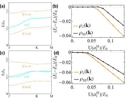
Figure 3: (a) The spectra for the Hartree-Fock mean-field Hamiltonian with the order parameter $\rho_{z}({\textbf{{k}}})$ at half filling of CB1 for the case with $\phi=0,\alpha=1,V_{0}/E_{0}=0$. $C$ is the Chern number of each band. (b) The difference in energy per particle between the self-consistent Hartree-Fock states $E_{i}$ and the non-interacting state $E_{n}$ as a function of Coulomb interaction strengths for the order parameters $\rho_{z}({\textbf{{k}}})$ (orange) and $\rho_{xy}({\textbf{{k}}})$ (black). (c) The spectra for the Hartree-Fock mean-field Hamiltonian with the order parameter $\rho_{z}({\textbf{{k}}})$ at half filling of CB1 for the case with $\phi=0,\alpha=0,V_{0}/E_{0}=1.2$. (d) The energy difference $E_{i}-E_{n}$ for the order parameters $\rho_{z}({\textbf{{k}}})$ (orange) and $\rho_{xy}({\textbf{{k}}})$ (black).

Interaction-driven QAH state $-$ The Coulomb interaction of electrons in the moiré superlattice can be estimated as $U_{0}=e^{2}/4\pi\varepsilon_{0}\varepsilon_{r}|{\textbf{{a}}}_{1}^{M}|\approx 5.11$meV $\sim 0.13E_{0}$, in which $e$ is the electron charge, $\varepsilon_{0}$ is vacuum permittivity, and dielectric constant $\varepsilon_{r}$ is about 10. Bernevig et al. (2021) The value of $U_{0}$ is comparable to both the moiré mini-band width $\sim 0.1E_{0}\approx 3.85$ meV and mini-band gaps $\sim 0.1E_{0}$. We next study the effects of the Coulomb interaction with the Hartree-Fock mean-field theoryZhang et al. (2020); Lian et al. (2021); Liu et al. (2021); Xie and MacDonald (2020); Bultinck et al. (2020); Bernevig et al. (2021). We first project the moiré Hamiltonian and the Coulomb interaction into the low-energy subspace spanned by either CB1 (a two-band model) or both CB1 and CB2 (a four-band model). By treating the density matrix $\rho_{n_{1}n_{2}}({\textbf{{k}}})=\langle c^{\dagger}_{n_{1}}({\textbf{{k}}})c_{n_{2}}({\textbf{{k}}})\rangle$ as the order parameter with $c^{\dagger}_{n}({\textbf{{k}}})$ for the creation operator of the $n$th eigenstate in the two-band or four-band subspace, we can decompose the Coulomb interaction Hamiltonian into two-fermion terms so that the order parameter $\rho({\textbf{{k}}})$ can be solved self-consistently (See SM Sec.II).

In the two-band model, we generally consider two types of order parameters, (1) $\rho_{z}({\textbf{{k}}})\propto f_{z}({\textbf{{k}}})\sigma_{z}$ and (2) $\rho_{xy}({\textbf{{k}}})\propto f_{x}({\textbf{{k}}})\sigma_{x}+f_{y}({\textbf{{k}}})\sigma_{y}$, where the $\sigma$ matrix is for the Kramers’ pair of CB1 and $f_{x,y,z}({\textbf{{k}}})$ represents the momentum-dependent part of the order parameter. The order parameter $\rho_{0}\propto\sigma_{0}$ is directly related to the band occupation and we always consider half-filling for the Kramers’ pair bands of CB1. At $\phi=0,\alpha=1,V_{0}/E_{0}=0$, the spin basis of CB1 also corresponds to mirror eigen-values $\pm i$ of horizontal mirror symmetry $\mathcal{M}_{z}$ of $D_{6h}$ group, and these two mirror-eigenstates carry nonzero mirror Chern number $\pm 1$ from the nontrivial $\mathbb{Z}_{2}$ topology. Thus, $\rho_{z}({\textbf{{k}}})$ and $\rho_{xy}({\textbf{{k}}})$ correspond to the mirror-polarized and mirror-coherent ground states. The self-consistent calculations suggest that both $\rho_{z}({\textbf{{k}}})$ and $\rho_{xy}({\textbf{{k}}})$ can be non-zero solutions when the Coulomb interaction exceeds certain critical values $U_{c}\sim 0.05E_{0}\approx 1.92$ meV, as shown in Fig. 3(b), where the ground state energies of self-consistent $\rho_{z}({\textbf{{k}}})$ and $\rho_{xy}({\textbf{{k}}})$ are shown as a function of interaction strength $U(a_{1}^{\text{M}})$, which is treated as a tuning parameter and equal to $U_{0}$ for the realistic moiré superlattice. Our estimate of Coulomb interaction $0.13E_{0}$ in TI moiré systems is larger than this critical value. From Fig. 3(b), we also see that the mirror-polarized state $\rho_{z}({\textbf{{k}}})$ has a lower ground state energy than the mirror-coherent state $\rho_{xy}({\textbf{{k}}})$. The energy spectrum of the CB1 before (blue lines) and after (orange lines) taking into account the $\rho_{z}({\textbf{{k}}})$ order parameter is shown in Fig. 3(a), in which the metallic state of CB1 (blue lines) is fully gapped out by $\rho_{z}({\textbf{{k}}})$ at half-filling. Due to non-zero mirror Chern number of non-interacting CB1 state, the mirror-polarized state $\rho_{z}({\textbf{{k}}})$ carries Chern number $\pm 1$ and thus gives rise to the QAH state. As shown in SM Sec.II.C, the mirror coherent state $\rho_{xy}({\textbf{{k}}})$ has nodes in its spectrum due to the $C_{2z}{\mathcal{T}}$ symmetry. This explains why the mirror-polarized state has a lower ground state energy than the mirror-coherent state. Thus, the mirror-polarized QAH state can be driven by Coulomb interaction in this system.

We also studied the case of $\phi=0,\alpha=0,V_{0}/E_{0}=1.2$ within the two-band model, in which the mirror $\mathcal{M}_{z}$ is broken at the single particle level and six-fold rotation remains, in SM Sec.II.C and find the $\rho_{z}({\textbf{{k}}})$ is still energetically favored, as shown in Fig. 3(d). The spectra with the order parameter $\rho_{z}({\textbf{{k}}})$ is shown in Fig. 3(c) and the ground state is a Chern insulator.

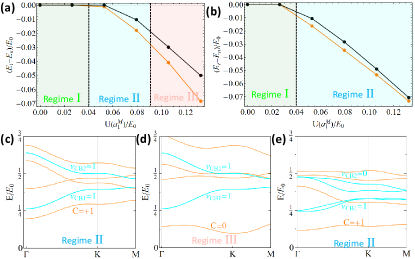
Figure 4: (a)The energy difference per particle $E_{i}-E_{n}$ at $1/4$ filling of the four-band model with both CB1 and CB2 for the case $\phi=0,\alpha=1,V_{0}/E_{0}=0$. Here $E_{i}$ and $E_{n}$ is the interacting ground state energy and non-interacting metallic state energy, respectively. The orange (black) line is for the $C_{2}\mathcal{T}$ symmetry breaking (preserving) density matrix. The interacting ground states in the regime I, II, and III correspond to a metallic phase, an insulating phase with $C=\pm 1$, and an insulating phase with $C=0$, respectively. (b) $E_{i}-E_{n}$ for the case with $\phi=0,\alpha=0,V_{0}/E_{0}=1.2$. (c)(d) The spectra of the Hartree-Fock mean-field Hamiltonian for the Coulomb interaction strength in regime II and III of (a). $C$ is the Chern number of each band. The spectra for the Hartree-Fock mean-field Hamiltonian for the case with $\phi=0,\alpha=1,V_{0}/E_{0}=0$. (e) The spectra of the mean-field Hamiltonian for the Coulomb interaction strength in Regime II of (b).

As the mini-band gap is comparable to Coulomb interaction, one may ask if the inter-mini-band mixing due to Coulomb interaction can change the topological nature of the ground state. Thus, we study the Coulomb interaction effect in a four-band model including both CB1 and CB2, as discussed in SM Sec.II.D. For the inversion-symmetric case $\phi=0,\alpha=1,V_{0}/E_{0}=0$, the ground state of the four-band model is still the mirror polarized $C=\pm 1$ state in regime II (blue) of Fig. 4(a), when $U(a_{1}^{\text{M}})=0.08E_{0}$ is smaller than the mini-band gap $\sim 0.1E_{0}$, with the spectra shown in Fig. 4(c). When $U(a_{1}^{\text{M}})=0.13E_{0}$ is larger than the mini-band gap (regime III (red) of Fig. 4(a)), the strong Coulomb interaction can induce mixing between CB1 and CB2 within one mirror parity sector and drive a topological phase transition to the $C=0$ state shown in Fig. 4(d) (More details in SM Sec.II.D). However, the situation for the inversion-asymmetric case $\phi=0,\alpha=0,V_{0}/E_{0}=1.2$ is different as $\nu_{\text{CB1}}=1$ and $\nu_{\text{CB2}}=0$. For the realistic estimated value $U(a_{1}^{\text{M}})\approx 0.13E_{0}$ that is larger than mini-band gap, the interacting ground state of the four-band model carries $C=\pm 1$ and thus remains the same as that of the two-band model, as shown by the regime II (blue) in Fig. 4(b). The energy spectra in this case is shown in Fig. 4(e). By comparing the phase diagrams for the inversion symmetric and asymmetric cases, we conclude that the asymmetric potential $V_{0}$ stabilizes the interaction-driven QAH state in TI moiré heterostructures.

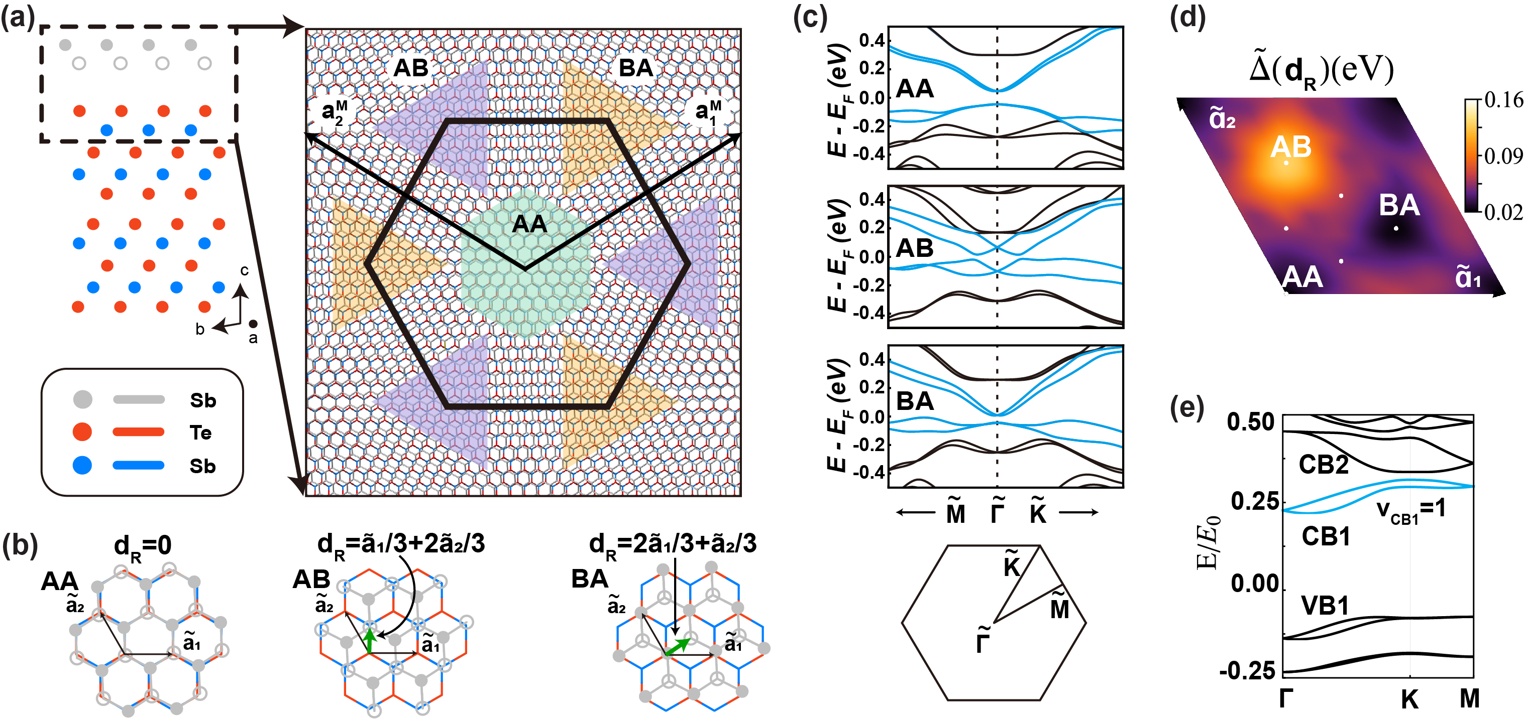
Figure 5: (a) Side view of Sb₂/2QL Sb₂Te₃ heterostructure with AA stacking (left panel) and the moiré pattern for twisted Sb₂ on top of Sb₂Te₃ thin film (right panel). To show the moiré pattern clearly, we only plot atoms in the region marked by black dashed lines in the left panel. The triangle regions with green, purple, and yellow background label structures with AA, AB, and BA stacking respectively. The primitive vectors for moiré supercell $a_{1}^{M}$ and $a_{2}^{M}$ are marked by black arrows. (b) Top views of configurations with AA, AB, and BA stacking. The atomic primitive lattice vectors of the 2QL Sb₂Te₃ thin film are labeled as $\tilde{{\textbf{{a}}}}_{1}\text{ and }\tilde{{\textbf{{a}}}}_{2}$. The green arrow labels the shift ${\textbf{{d}}}_{\textbf{{R}}}$ between the Sb₂Te₃ layer and Sb₂ monolayer in each stacked configuration. (c) Band structures around the $\Gamma$ point for heterostructures with AA, AB, and BA stacking from DFT calculations. The Brillouin zone is plotted for the slab model used in DFT calculations with atomic primitive lattices. The Fermi levels are set as zero. (d) The superlattice potential $\tilde{\Delta}({\textbf{{d}}}_{R})$ as a function of ${\textbf{{d}}}_{R}$ shown in the moiré superlattice. $\tilde{{\textbf{{a}}}}_{1,2}$ are marked by the black arrows. (e) Energy spectrum for twisted monolayer Sb₂ and 2QL Sb₂Te₃ with the superlattice potential shown in (d).

Sb₂/Sb₂Te₃ moiré heterostructure.$-$ We propose a possible experimental realization of TI based moiré heterostructure with twisted Sb₂ monolayer on top of Sb₂Te₃ thin film. The moiré lattice structure is shown in Fig. 5(a). Sb₂Te₃ is a prototype of three dimensional TI with layered structures. Within one quintuple layer (QL, see the red and green dots in Fig. 5(a)), there is strong chemical binding formed by the sequential Te-Sb-Te-Sb-Te atomic layers and the van der Waals coupling is between adjacent QLs Zhang et al. (2009). Precise control of layer thickness of the Sb₂Te₃ thin film has been achieved via molecular beam epitaxy (MBE) method experimentallyJiang et al. (2012); Zhang et al. (2013). On the top of Sb₂Te₃ thin film, Sb₂ monolayer could be depositedZhu et al. (2019); Bian et al. (2012); Chang et al. (2015b), forming Sb₂/Sb₂Te₃ heterostructure. By using density functional theory (DFT) calculations, we confirm that Sb₂ monolayer with buckled honeycomb structure marked as the gray in Fig. 5(a) is a semiconductor with a band gap larger than that of Sb₂Te₃ thin films. Furthermore, we put Sb₂ monolayer on the top of 2QL Sb₂Te₃ thin films with different stackings, including the AA, AB, and BA stackings (see Fig. 5(a)). The corresponding electronic band structures are shown in Fig. 5(c). The work function of monolayer Sb₂ and Sb₂Te₃ thin film matches with each other, forming the type I semiconductor hetero-junction. Around the Fermi level, the conduction and valence bands are both mainly contributed by two strongly hybridized surface states of the 2QL Sb₂Te₃ thin film. The role of Sb₂ monolayer is to provide a potential along the out-of-plane direction, leading to a Rashba type of spin-split bands. Thus, the twisted Sb₂/Sb₂Te₃ moiré heterostructure satisfies the requirements mentioned above for the $\mathbb{Z}_{2}$ nontrivial moiré minibands.

To connect the theoretical moiré model Hamiltonian in Eq. (1) to electronic band structure from DFT calculations, we first introduce a uniform shifting vector ${\textbf{{d}}}_{\textbf{{R}}}$ between monolayer Sb₂ and 2QL Sb₂Te₃ thin film, and AA, AB, and BA stackings correspond to ${\textbf{{d}}}_{R}=0,\tilde{{\textbf{{a}}}}_{1}/3+2\tilde{{\textbf{{a}}}}_{2}/3,\text{ and }2\tilde{{\textbf{{a}}}}_{1}/3+\tilde{{\textbf{{a}}}}_{2}/3$, respectively (Fig. 5(b)). $\tilde{{\textbf{{a}}}}_{1,2}$ are atomic primitive lattice vectors for Sb₂Te₃ lattice shown in Fig. 5(b). The spectrum from DFT calculations with different stacking is fitted by the dispersion of two-surface-state atomic Hamiltonian

$$\begin{split}H^{\text{DFT}}&({\textbf{{k}}},{\textbf{{d}}}_{\textbf{{R}}})=H^{\text{TI}}({\textbf{{k}}})\\ &+\frac{1+\alpha}{2}\tilde{\Delta}({\textbf{{d}}}_{\textbf{{R}}})\tau_{0}s_{0}+\frac{1-\alpha}{2}\tilde{\Delta}({\textbf{{d}}}_{\textbf{{R}}})\tau_{z}s_{0},\end{split}$$ (3)

where $s_{0}(\tau_{0,z})$ are the Pauli matrices for the spin (surfaces). $\tilde{\Delta}({\textbf{{d}}}_{\textbf{{R}}})$ is a uniform atomic potential induced by the Sb₂ monolayer for a fixed ${\textbf{{d}}}_{\textbf{{R}}}$ and different ${\textbf{{d}}}_{\textbf{{R}}}$ values correspond to different stacking configurations, shown in Fig. 5(b). For the ${\textbf{{d}}}_{\textbf{{R}}}$ values corresponding to the AA, AB, BA and several other stackings in SM Sec.III, we fit the energy dispersion of the model Hamiltonian $H^{\text{DFT}}({\textbf{{k}}},{\textbf{{d}}}_{\textbf{{R}}})$ to that from the DFT calculations to extract $\tilde{\Delta}({\textbf{{d}}}_{\textbf{{R}}})$, which can be further interpolated as a continuous function of ${\textbf{{d}}}_{\textbf{{R}}}$ shown in Fig. 5(d). $\tilde{\Delta}({\textbf{{d}}}_{\textbf{{R}}})$ has the periodicity of the atomic unit-cell defined by $\tilde{{\textbf{{a}}}}_{1,2}$. All other parameters in $H^{\text{DFT}}({\textbf{{k}}},{\textbf{{d}}}_{\textbf{{R}}})$ are treated as constants and can also obtained by fitting to the DFT bands. After obtaining the parameters for $H^{\text{DFT}}({\textbf{{k}}},{\textbf{{d}}}_{\textbf{{R}}})$, the next step is to connect them to those of the moiré Hamiltonian $H_{0}$ in Eq. (1). For the moiré TI with the twist angle $\theta$, the local shift between two layers at the atomic lattice vector R of the Sb₂Te₃ layer is ${\textbf{{d}}}_{\textbf{{R}}}=\mathcal{R}(\theta){\textbf{{R}}}-{\textbf{{R}}}$ , where $\mathcal{R}(\theta)$ is the rotation operator, so we can obtain the potential

$$\Delta({\textbf{{R}}})\approx\tilde{\Delta}({\textbf{{d}}}_{\textbf{{R}}})$$ (4)

at the location R. The last step is to treat $\Delta({\textbf{{r}}})$ as a function of continuous r by interpolating the function $\Delta({\textbf{{R}}})$ (See SM.IV), and $\Delta({\textbf{{r}}})$ serves as the morié superlattice potential for the model Hamiltonian $H_{0}({\textbf{{r}}})$. Besides, all the other parameters in $H_{0}$ are chosen to be the same as those in $H^{\text{DFT}}$. In Fig. 5(d), the potential maximum of $\tilde{\Delta}({\textbf{{d}}}_{\textbf{{R}}})$ appears at the AB stacking while two local minima exist at the BA and AA stackings and are close in energy. The parameters for the moiré potential at $\theta=0.5^{\circ}$ is given by $\Delta_{1}/E_{0}=0.22,\alpha=0.16$, and $\phi=0.68\pi$, close to $\phi=2\pi/3$ for the $C_{6}$-rotation symmetric potential in Fig. 2(g). Fig. 5(e) shows the energy dispersion of moiré mini-bands for $V_{0}/E_{0}=1.2$, in which the lowest conduction bands (cyan) indeed are isolated mini-bands with nontrivial $\nu_{CB1}$=1.

Conclusion and Discussion $-$ In summary, we demonstrate that the superlattice potential in a TI thin film can give rise to $\mathbb{Z}_{2}$ non-trivial isolated moiré mini-bands and Coulomb interaction can drive the system into the QAH state when the Kramer’s pair of non-trivial mini-bands are half filled. Besides the twisted Sb₂ monolayer on top of Sb₂Te₃ thin film, our model can be generally applied to other TI heterostructures with the in-plane superlattice potential, which can come from either the moiré pattern of another 2D insulating material or by gating a periodic patterned dielectric substrateForsythe et al. (2018); Yankowitz et al. (2018); Li et al. (2021); Shi et al. (2019); Xu et al. (2021a). The 2D TI thin films can be in a quantum spin Hall state or trivial insulator state, depending on the relative sign between $m_{0}$ and $m_{2}$ in the model Hamiltonian (see Eq. (1)) Liu et al. (2010b). Our calculations suggest that the Moiré potential can lead to $\mathbb{Z}_{2}$ non-trivial mini-bands no matter the sign of $m_{2}$, once this term is negligible compared to the linear term in the moiré scale. Such a result implies the possibility of realizing isolated $\mathbb{Z}_{2}$ non-trivial mini-bands in other 2D topologically trivial systems with strong Rashba SOC. In our calculation, a large moiré superlattice constant ($|{\textbf{{a}}}_{1}^{\text{M}}|\sim 28$nm) leads to small energy scales, around a few meV, for mini-band widths, mini-band gaps and Coulomb interactions, which may be disturbed by disorders. In See SM Sec.II.E, we reduce $|{\textbf{{a}}}_{1}^{\text{M}}|$ to $\sim 14$nm, which yields larger energy scales (around $10$meV) of mini-bands and Coulomb interaction, and our Hartree-Fock calculations suggests the estimated Coulomb interaction is still strong enough to drive the system into the QAH state. For a smaller moiré lattice constant $|{\textbf{{a}}}_{1}^{\text{M}}|$, it is desirable to reduce the bandwidth of moiré mini-bands while keeping the Coulomb energy, and this can be achieved by twisting two identical TIs or with in-plane magnetic fields, as proposed recently Chaudhary et al. (2022); Dunbrack and Cano (2022).

Acknowledgement – We would like to acknowledge Liang Fu, Jainendra Jain, Ribhu Kaul, Binghai Yan, Yunzhe Liu, Lunhui Hu and Jiabin Yu for the helpful discussion. KJY and CXL acknowledge the support through the Penn State MRSEC–Center for Nanoscale Science via NSF award DMR-2011839. CXL and BAB also acknowledges the support from the Princeton NSF-MERSEC (Grant No. MERSEC DMR 2011750). FS was supported by a fellowship at the Princeton Center for Theoretical Science. BAB was furthermore supported by Simons Investigator Grant No. 404513, ONR Grant No. N00014-20-1-2303, the Schmidt Fund for Innovative Research, the BSF Israel US Foundation Grant No. 2018226, the Gordon and Betty Moore Foundation through Grant No. GBMF8685 towards the Princeton theory program and Grant No. GBMF11070 towards the EPiQS Initiative, and the Princeton Global Network Fund. BAB acknowledges additional support through the European Research Council (ERC) under the European Union’s Horizon 2020 research and innovation program (Grant Agreement No. 101020833). PZT was supported by the National Natural Science Foundation of China (Grants No. 12234011) and the Open Research Fund Program of the State Key Laboratory of Low-Dimensional Quantum Physics.

Supplemental Materials

I Topology of the lowest conduction bands

I.1 Perturbation Theory and emergent chiral symmetry

In this section, the topology of inversion symmetric moiré system in Fig. 2(a) of the main text with $\phi=0,\alpha=1,V_{0}/E_{0}=0$ is studied under the perturbation of moiré potential strength $\Delta_{1}$.

By the Fu-Kane parity criterionFu and Kane (2007), the $\mathbb{Z}_{2}$ invariant $\nu$ can be determined by the parities $\lambda_{i}$ at time reversal ($\mathcal{T}$) invariant momenta one $\Gamma$ and three M of moiré Brillouin Zone (MBZ) for one of the degenerate states by $(-1)^{\nu}=\prod_{i}\lambda_{i}$ At $\phi=0,\alpha=1,V_{0}/E_{0}=0$, the crystal symmetry of this system is described by the point group $D_{6h}$ with six-fold rotation $C_{6z}$ about the z-axis, the inversion $\mathcal{I}$, the y-directional mirror $\mathcal{M}_{y}$ and the z-directional mirror $\mathcal{M}_{z}$. We label the original basis of our model Hamiltonian Eq. 1 in main text by $|{{\textbf{{k}}}},J_{z},\alpha\rangle$, where k is the momentum, $J_{z}=\pm 1/2$ labels two spin states of surface states and $\alpha=\text{t},\text{b}$ labels the top and bottom surfaces. The z-directional mirror $\mathcal{M}_{z}$ transforms the top surface to the bottom surface and thus it relates the basis wave-functions on two surfaces by

$$\mathcal{M}_{z}|{\textbf{{k}}},J_{z},\text{t}\rangle=e^{-i\pi J_{z}}|{\textbf{{k}}},J_{z},\text{b}\rangle\quad\mathcal{M}_{z}|{\textbf{{k}}},J_{z},\text{b}\rangle=e^{-i\pi J_{z}}|{\textbf{{k}}},J_{z},\text{t}\rangle.$$ (S1)

We may transform the basis wave-functions to the bonding and anti-bonding states of two surface states as

$$|{\textbf{{k}}},J_{z},I\rangle=\frac{1}{\sqrt{2}}(|{\textbf{{k}}},J_{z},\text{t}\rangle+I|{\textbf{{k}}},J_{z},\text{b}\rangle)$$ (S2)

with $I=\pm$ labels the transformation property under the inversion parity

$$\mathcal{I}|{\textbf{{k}}},J_{z},\pm\rangle=\pm|-{\textbf{{k}}},J_{z},\pm\rangle$$ (S3)

and the eigen-values of the $\mathcal{M}_{z}$ operator

$$\mathcal{M}_{z}|{\textbf{{k}}},J_{z},\pm\rangle=\pm e^{-i\pi J_{z}}|{\textbf{{k}}},J_{z},\pm\rangle.$$ (S4)

On these bonding and anti-bonding basis

$$|{\textbf{{k}}},J_{z},I\rangle=|{\textbf{{k}}},+\frac{1}{2},+\rangle,|{\textbf{{k}}},-\frac{1}{2},-\rangle,|{\textbf{{k}}},-\frac{1}{2},+\rangle,|{\textbf{{k}}},+\frac{1}{2},-\rangle,$$ (S5)

the Hamiltonian $H_{0}$ in the main text Eq.1 can be written in a block diagonal form,

$$H_{0}({\textbf{{r}}})=H^{\text{TI}}+H^{\text{M}}({\textbf{{r}}})=\begin{pmatrix}H^{\text{TI}}_{m_{z}=-i}&0\\ 0&H^{\text{TI}}_{m_{z}=+i}\\ \end{pmatrix}+\Delta({\textbf{{r}}})I_{4\times 4}.$$ (S6)

with

$$H^{\text{TI}}_{m_{z}=\pm i}=\begin{pmatrix}m&\mp iv\hat{k}_{\pm}\\ \pm iv\hat{k}_{\mp}&-m\\ \end{pmatrix},$$ (S7)

where $\hat{k}_{\pm}=-i(\partial_{x}\pm i\partial_{y})$, $m=m_{0}+m_{2}(-\partial_{x}^{2}-\partial_{y}^{2})$, $I_{4\times 4}$ is a $4\times 4$ identity matrix, and $m_{z}=\pm i$ labels the eigen-values of the mirror operator $\mathcal{M}_{z}$. $H^{\text{M}}$ is the moiré potential with $\phi=0,\alpha=1,V_{0}/E_{0}=0$.

We next determine the parities of lower-energy mini-bands at $\mathcal{T}$ invariant momenta, including one $\Gamma$ and three $M$ in the moiré BZ, of the Hamiltonian $H_{0}$ in the limit $|\Delta_{1}|\ll|v{\textbf{{b}}}_{1}^{\text{M}}|,|m|$ via perturbation theory. As the $H_{0}$ is block diagonal in the $m_{z}=\pm i$ subspace, we may perform the perturbation calculation for the $m_{z}=-i$ block while the mini-band parity of the $m_{z}=+i$ block can be related by TR symmetry. For the $m_{z}=-i$ block, the unperturbed Hamiltonian is $H^{\text{TI}}_{m_{z}=-i}$ while $H^{\text{M}}$ is treated as the perturbation. We choose the eigen-wavefunctions of $H^{\text{TI}}_{m_{z}=-i}$ to possess a well-defined gauge at $\Gamma$ in the moiré BZ, which can be written as

$$|\psi^{\text{TI}}_{+,-i}({\textbf{{k}}})\rangle=\begin{pmatrix}i\cos\frac{\theta_{\textbf{{k}}}}{2}\\ \sin\frac{\theta_{\textbf{{k}}}}{2}e^{i\phi_{\textbf{{k}}}}\end{pmatrix}\quad|\psi^{\text{TI}}_{-,-i}({\textbf{{k}}})\rangle=\begin{pmatrix}-i\sin\frac{\theta_{k}}{2}e^{-i\phi_{k}}\\ \cos\frac{\theta_{k}}{2}\\ \end{pmatrix}$$ (S8)

for $m>0$ with the eigen-energies $E^{\text{TI}}_{\pm}({\textbf{{k}}})=\pm\sqrt{m^{2}+v^{2}k^{2}}$ and

$$|\psi^{\text{TI}}_{+,-i}({\textbf{{k}}})\rangle=\begin{pmatrix}i\sin\frac{\theta_{k}}{2}\\ -\cos\frac{\theta_{k}}{2}e^{i\phi_{k}}\\ \end{pmatrix}\quad|\psi^{\text{TI}}_{-,-i}({\textbf{{k}}})\rangle=\begin{pmatrix}i\cos\frac{\theta_{\textbf{{k}}}}{2}e^{-i\phi_{\textbf{{k}}}}\\ \sin\frac{\theta_{\textbf{{k}}}}{2}\end{pmatrix}$$ (S9)

for $m<0$ with the eigen-energies $E^{\text{TI}}_{\pm}({\textbf{{k}}})=\mp\sqrt{m^{2}+v^{2}k^{2}}$, where $\cos\theta_{k}=m/\sqrt{m^{2}+v^{2}k^{2}}$ and $ke^{i\phi_{k}}=k_{x}+ik_{y}$.

$$\mathcal{I}|\psi^{\text{TI}}_{I,-i}({\textbf{{k}}})\rangle=I|\psi^{\text{TI}}_{I,-i}(-{\textbf{{k}}})\rangle,$$ (S10)

and the expression for the eigen-energy can be unified as

$$E^{\text{TI}}_{I}({\textbf{{k}}})={\text{sgn}(m)}I\sqrt{m^{2}+v^{2}k^{2}},$$ (S11)

so the inversion parity $I$ also labels different eigen-energies of our model Hamiltonian. The second lower-index $-i$ in the eigen-state labels the $\mathcal{M}_{z}$ eigen-values. This definition of the eigen-states $|\psi^{\text{TI}}_{I,m_{z}}\rangle$ is also used in the main text. From the expression of the eigen-energies (S11), the higher energy state with $E^{\text{TI}}_{\text{CB}}({\textbf{{k}}})=E^{\text{TI}}_{I=+\text{sgn}(m)}({\textbf{{k}}})$ that corresponds to the conduction bands should be given by

$$|\psi^{\text{TI}}_{\text{CB},-i}({\textbf{{k}}})\rangle=|\psi^{\text{TI}}_{+\text{sgn}(m),-i}({\textbf{{k}}})\rangle$$ (S12)

and the lower energy state with $E^{\text{TI}}_{\text{VB}}({\textbf{{k}}})=E^{\text{TI}}_{I=-\text{sgn}(m)}({\textbf{{k}}})$ for the valence bands should be

$$|\psi^{\text{TI}}_{\text{VB},-i}({\textbf{{k}}})\rangle=|\psi^{\text{TI}}_{-\text{sgn}(m),-i}({\textbf{{k}}})\rangle.$$ (S13)

For $m_{z}=+i$ subspace, we use TR symmetry operator, given by

$$\mathcal{T}=\begin{pmatrix}0&0&-1&0\\ 0&0&0&1\\ 1&0&0&0\\ 0&-1&0&0\\ \end{pmatrix}\mathcal{K}$$ (S14)

in the basis Eq. (S5) with $\mathcal{K}$ for complex conjugate, to define

$$|\psi^{\text{TI}}_{I,+i}({\textbf{{k}}})\rangle=-i\mathcal{T}|\psi^{\text{TI}}_{I,-i}(-{\textbf{{k}}})\rangle,$$ (S15)

and the commutation relation $[\mathcal{T},\mathcal{I}]=0$ leads to the same inversion parity for two degenerate states $|\psi^{\text{TI}}_{I,m_{z}=\pm i}(\Gamma_{i})\rangle$ at any TR-invariant momentum $\Gamma_{i}$.

The band gap and the inversion parity of mini-bands at $\Gamma$ of the moiré BZ are determined by the hybridization term $m$ in the limit $|\Delta_{1}|\ll|m|$, for which the moiré potential does not play a role. Thus, we only need to consider the unperturbed Hamiltonian $H^{\text{TI}}_{m_{z}=-i}$ in Eq. (S7), which is diagonal, and the eigen-state $|\psi^{\text{TI}}_{+,-i}(\Gamma)\rangle=(1,0)^{T}$ has the eigen-energy $m$ and $|\psi^{\text{TI}}_{-,-i}(\Gamma)\rangle=(0,1)^{T}$ has the eigen-energy $-m$. The lower index $I$ directly gives the parity of the eigen-state at $\Gamma$, namely $\mathcal{I}|\psi^{\text{TI}}_{I,-i}(\Gamma)\rangle=I|\psi^{\text{TI}}_{I,-i}(\Gamma)\rangle$. The parity of the CB1 for the eigen-state $|\psi^{\text{TI}}_{\text{CB},-i}(\Gamma)\rangle$ is $\lambda_{\Gamma}=+\text{sgn}(m)$ and that of the VB1 for the eigen-state $|\psi^{\text{TI}}_{\text{VB},-i}(\Gamma)\rangle$ is $\lambda_{\Gamma}=-\text{sgn}(m)$, depending on the sign of $m$. Therefore, the parities of CB1 and VB1 at $\Gamma$ are opposite,

$$\lambda^{\text{CB1}}_{\Gamma}=-\lambda^{\text{VB1}}_{\Gamma}.$$ (S16)

Different from the $\Gamma$ point, the moiré potential is essential in determining the parities of the mini-bands at $M$ in the moiré BZ. Without moiré potential, the eigen-states $|\psi^{\text{TI}}_{I,-i}({\textbf{{k}}})\rangle$ of $H^{\text{TI}}_{m_{z}=-i}$ at ${\textbf{{k}}}={\textbf{{M}}}=\frac{1}{2}{\textbf{{b}}}_{1}^{\text{M}}$ and ${\textbf{{k}}}={\textbf{{M}}}-{\textbf{{b}}}_{1}^{\text{M}}=-{\textbf{{M}}}$ are degenerate, so the spectrum is gapless at M, even with a finite $m$. The moiré potential will couple these two states at M and $-{\textbf{{M}}}$ as both belong to the same momentum in moiré BZ. By projecting the full Hamiltonian $H_{0}({\textbf{{r}}})$ into the subspace spanned by these two states $|\psi^{\text{TI}}_{\text{CB},-i}(\pm{\textbf{{M}}})\rangle$, we find the effective Hamiltonian $H^{\text{CB}}_{eff}({\textbf{{M}}})$ for CB1 and CB2 is given through the degenerate perturbation by

$$\begin{split}H^{\text{CB}}_{eff}({\textbf{{M}}})&=\begin{pmatrix}\langle\psi^{\text{TI}}_{\text{CB},-i}({\textbf{{M}}})|H^{\text{TI}}|\psi^{\text{TI}}_{\text{CB},-i}({\textbf{{M}}})\rangle&\langle\psi^{\text{TI}}_{\text{CB},-i}({\textbf{{M}}})|H^{\text{M}}|\psi^{\text{TI}}_{\text{CB},-i}(-{\textbf{{M}}})\rangle\\ \langle\psi^{\text{TI}}_{\text{CB},-i}(-{\textbf{{M}}})|H^{\text{M}}|\psi^{\text{TI}}_{\text{CB},-i}({\textbf{{M}}})\rangle&\langle\psi^{\text{TI}}_{\text{CB},-i}(-{\textbf{{M}}})|H^{\text{TI}}|\psi^{\text{TI}}_{\text{CB},-i}(-{\textbf{{M}}})\rangle\end{pmatrix}\\ &=\begin{pmatrix}E^{\text{TI}}_{\text{CB}}({\textbf{{M}}})&\Delta_{1}|\cos\theta_{k_{\text{M}}}|\\ \Delta_{1}|\cos\theta_{k_{\text{M}}}|&E^{\text{TI}}_{\text{CB}}(-{\textbf{{M}}})\end{pmatrix},\end{split}$$ (S17)

where $E^{\text{TI}}_{\text{CB}}({\textbf{{M}}})=E^{\text{TI}}_{\text{CB}}(-{\textbf{{M}}})=\sqrt{m^{2}+v^{2}k_{\text{M}}^{2}},\cos\theta_{k_{\text{M}}}=m/\sqrt{m^{2}+v^{2}k_{\text{M}}^{2}}$, and $k_{\text{M}}=|{\textbf{{M}}}|$. The eigen-state $(|\psi^{\text{TI}}_{\text{CB},-i}({\textbf{{M}}})\rangle+|\psi^{\text{TI}}_{\text{CB},-i}(-{\textbf{{M}}})\rangle)/\sqrt{2}$ has eigen-energy $E^{\text{TI}}_{\text{CB}}({\textbf{{M}}})+\Delta_{1}|\cos\theta_{\textbf{{k}}}|$ and the parity $+\text{sgn}(m)$ while the eigen-state $(|\psi^{\text{TI}}_{\text{CB},-i}({\textbf{{M}}})\rangle-|\psi^{\text{TI}}_{\text{CB},-i}(-{\textbf{{M}}})\rangle)/\sqrt{2}$ has eigen-energy $E^{\text{TI}}_{\text{CB}}({\textbf{{M}}})-\Delta_{1}|\cos\theta_{\textbf{{k}}}|$ and the parity $-\text{sgn}(m)$. The lower energy state (eigen-energy $E^{\text{TI}}_{\text{CB}}({\textbf{{M}}})-|\Delta_{1}||\cos\theta_{\textbf{{k}}}|$), which corresponds to CB1, depends on the sign of $\Delta_{1}$ and is given by

$$|\psi_{\text{CB1},-i}({\textbf{{M}}})\rangle=(|\psi^{\text{TI}}_{\text{CB},-i}({\textbf{{M}}})\rangle-\text{sgn}(\Delta_{1})|\psi^{\text{TI}}_{\text{CB},-i}(-{\textbf{{M}}})\rangle)/\sqrt{2}$$ (S18)

with the parity $\lambda^{\text{CB1}}_{\textbf{{M}}}=(+\text{sgn}(m))(-\text{sgn}(\Delta_{1}))$. For VB1 and VB2, the effective Hamiltonian at M is given by

$$\begin{split}H^{\text{VB}}_{eff}({\textbf{{M}}})&=\begin{pmatrix}\langle\psi^{\text{TI}}_{\text{VB},-i}({\textbf{{M}}})|H^{\text{TI}}|\psi^{\text{TI}}_{\text{VB},-i}({\textbf{{M}}})\rangle&\langle\psi^{\text{TI}}_{\text{VB},-i}({\textbf{{M}}})|H^{\text{M}}|\psi^{\text{TI}}_{\text{VB},-i}(-{\textbf{{M}}})\rangle\\ \langle\psi^{\text{TI}}_{\text{VB},-i}(-{\textbf{{M}}})|H^{\text{M}}|\psi^{\text{TI}}_{\text{VB},-i}({\textbf{{M}}})\rangle&\langle\psi^{\text{TI}}_{\text{VB},-i}(-{\textbf{{M}}})|H^{\text{TI}}|\psi^{\text{TI}}_{\text{VB},-i}(-{\textbf{{M}}})\rangle\end{pmatrix}\\ &=\begin{pmatrix}E^{\text{TI}}_{\text{VB}}({\textbf{{M}}})&\Delta_{1}|\cos\theta_{k_{\text{M}}}|\\ \Delta_{1}|\cos\theta_{k_{\text{M}}}|&E^{\text{TI}}_{\text{VB}}(-{\textbf{{M}}})\end{pmatrix},\end{split}$$ (S19)

where $E^{\text{TI}}_{\text{VB}}({\textbf{{M}}})=-\sqrt{m^{2}+v^{2}k_{\text{M}}^{2}}$. The eigen-state $(|\psi^{\text{TI}}_{\text{VB},-i}({\textbf{{M}}})\rangle+|\psi^{\text{TI}}_{\text{VB},-i}(-{\textbf{{M}}})\rangle)/\sqrt{2}$ has eigen-energy $E^{\text{TI}}_{\text{VB}}({\textbf{{M}}})+\Delta_{1}|\cos\theta_{k_{\text{M}}}|$ and the parity $-\text{sgn}(m)$ while the eigen-state $(|\psi^{\text{TI}}_{\text{VB},-i}({\textbf{{M}}})\rangle-|\psi^{\text{TI}}_{\text{VB},-i}(-{\textbf{{M}}})\rangle)/\sqrt{2}$ has eigen-energy $E^{\text{TI}}_{\text{VB}}({\textbf{{M}}})-\Delta_{1}|\cos\theta_{k_{\text{M}}}|$ and the parity $\text{sgn}(m)$. The higher energy state (eigen-energy $E^{\text{TI}}_{\text{VB}}({\textbf{{M}}})+|\Delta_{1}||\cos\theta_{k_{\text{M}}}|$), which corresponds to VB1, is given by

$$|\psi_{\text{VB1},-i}({\textbf{{M}}})\rangle=(|\psi^{\text{TI}}_{\text{VB},-i}({\textbf{{M}}})\rangle+\text{sgn}(\Delta_{1})|\psi^{\text{TI}}_{\text{VB},-i}(-{\textbf{{M}}})\rangle)/\sqrt{2}$$ (S20)

with the parity $\lambda^{\text{VB1}}_{{\textbf{{M}}}}=(-\text{sgn}(m))(+\text{sgn}(\Delta_{1}))$. Thus,

$$\lambda^{\text{CB1}}_{{\textbf{{M}}}}=\lambda^{\text{VB1}}_{{\textbf{{M}}}}=-\text{sgn}(m)\text{sgn}(\Delta_{1}).$$ (S21)

The parity at M for CB1 and VB1 are the same. Because the $\mathbb{Z}_{2}$ invariant is $(-1)^{\nu}=\lambda_{\Gamma}(\lambda_{\textbf{{M}}})^{3}$, $(-1)^{\nu_{\text{CB1}}}=-\text{sgn}(\Delta_{1})$ and $(-1)^{\nu_{\text{VB1}}}=+\text{sgn}(\Delta_{1})$, so that $\nu_{\text{CB1}}$ and $\nu_{\text{VB1}}$ are differed by 1. Thus, we conclude $\nu_{CB1}+\nu_{VB1}=1$ mod 2, namely one of CB1 and VB1 has nonzero $\mathbb{Z}_{2}$ invariant and the other has trivial $\mathbb{Z}_{2}$ invariant.

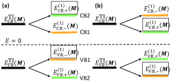
Figure S1: Schematic figures of energies under the first order perturbation. The orange (green) lines are states with odd (even) parities. The framed/unframed energies have the first order energy perturbation related by chiral symmetries. (a) $\langle\Psi_{\text{CB},+,m_{z}}({\textbf{{M}}})|H^{\text{M}}|\Psi_{\text{CB},+,m_{z}}({\textbf{{M}}})\rangle>\langle\Psi_{\text{CB},-,m_{z}}({\textbf{{M}}})|H^{\text{M}}|\Psi_{\text{CB},-,m_{z}}({\textbf{{M}}})\rangle$. (b) $\langle\Psi_{\text{CB},+,m_{z}}({\textbf{{M}}})|H^{\text{M}}|\Psi_{\text{CB},+,m_{z}}({\textbf{{M}}})\rangle<\langle\Psi_{\text{CB},-,m_{z}}({\textbf{{M}}})|H^{\text{M}}|\Psi_{\text{CB},-,m_{z}}({\textbf{{M}}})\rangle$ for $m_{z}=\pm i$.

The above conclusion of topology of CB1 and VB1 can also be understood from the chiral symmetry operator $\mathcal{C}$ of $H^{\text{TI}}$, defined by $\mathcal{C}=\tau_{z}s_{z}$, when the chemical potential is at the charge neutrality point, where $\tau$ acts on the top/bottom surface degrees of freedom and $s$ acts on spin. The emergence of the chiral symmetry requires dropping higher-order $k$ terms, e.g. $k^{2}$ terms, in $H^{\text{TI}}$, which are not important at the moiré energy scale. This operator has the commutation relations

$$\left\{\mathcal{C},H^{\text{TI}}\right\}=0,\left[\mathcal{C},H^{\text{M}}\right]=0,\left\{\mathcal{C},\mathcal{I}\right\}=0,\left\{\mathcal{C},\mathcal{M}_{z}\right\}=0.$$ (S22)

On the basis of Eq. (S5), the form of chiral symmetry operator is transformed into

$$\mathcal{C}=\begin{pmatrix}0&0&0&1\\ 0&0&-1&0\\ 0&-1&0&0\\ 1&0&0&0\\ \end{pmatrix},$$ (S23)

which mixes the eigen-states with opposite $\mathcal{M}_{z}$ eigen-values, namely

$$|\psi^{\text{TI}}_{-I,+i}({\textbf{{k}}})\rangle=\mathcal{C}|\psi^{\text{TI}}_{I,-i}({\textbf{{k}}})\rangle.$$ (S24)

This implies

$$|\psi_{\text{VB},+i}({\textbf{{k}}})\rangle=\mathcal{C}|\psi_{\text{CB},-i}({\textbf{{k}}})\rangle=\mathcal{C}|\psi^{\text{TI}}_{+\text{sgn}(m),-i}({\textbf{{k}}})\rangle=|\psi^{\text{TI}}_{-\text{sgn}(m),+i}({\textbf{{k}}})\rangle.$$ (S25)

At $\Gamma$, the opposite parities between $|\psi_{\text{CB},-i}(\Gamma)\rangle$ and $|\psi_{\text{VB},+i}(\Gamma)\rangle$ ($+\text{sgn}(m)$ for $|\psi_{\text{CB},-i}(\Gamma)\rangle$ and $-\text{sgn}(m)$ for $|\psi_{\text{VB},+i}(\Gamma)\rangle$ directly come from the anti-commutation relation $\left\{\mathcal{C},\mathcal{I}\right\}=0$.

At $M$, the CB1 (VB1) and CB2 (VB2) are degenerate for $H^{\text{TI}}$, so we need to consider the first order perturbation from $H^{\text{M}}$. For the convenience of the discussion, we introduce the inversion adapted basis functions for CB1, CB2, VB1, and VB2 as

$$\begin{split}|\Psi_{\text{CB},I,m_{z}}({\textbf{{M}}})\rangle&=\frac{1}{\sqrt{2}}\left(|\psi^{\text{TI}}_{\text{CB},m_{z}}({\textbf{{M}}})\rangle+I\text{sgn}(m)|\psi^{\text{TI}}_{\text{CB},m_{z}}(-{\textbf{{M}}})\rangle\right)\\ |\Psi_{\text{VB},I,m_{z}}({\textbf{{M}}})\rangle&=\frac{1}{\sqrt{2}}\left(|\psi^{\text{TI}}_{\text{VB},m_{z}}({\textbf{{M}}})\rangle-I\text{sgn}(m)|\psi^{\text{TI}}_{\text{VB},m_{z}}(-{\textbf{{M}}})\rangle\right)\end{split}$$ (S26)

with the parity

$$\mathcal{I}|\Psi_{\text{CB},I,m_{z}}\rangle=I|\Psi_{\text{CB},I,m_{z}}\rangle\quad\mathcal{I}|\Psi_{\text{VB},I,m_{z}}\rangle=I|\Psi_{\text{VB},I,m_{z}}\rangle.$$ (S27)

They are related by chiral symmetry

$$|\Psi_{\text{VB},I,m_{z}}({\textbf{{M}}})\rangle=\mathcal{C}|\Psi_{\text{CB},-I,-m_{z}}({\textbf{{M}}})\rangle.$$ (S28)

As $\left[\mathcal{I},H^{\text{M}}\right]=0$, the first order perturbation correction from $H^{\text{M}}$ is diagonal. For CB1 and CB2 $|\Psi_{\text{CB},I,m_{z}}({\textbf{{M}}})\rangle$, we find the perturbation Hamiltonian is

$$\begin{split}&\begin{pmatrix}\langle\Psi_{\text{CB},+,m_{z}}({\textbf{{M}}})|H^{\text{M}}|\Psi_{\text{CB},+,m_{z}}({\textbf{{M}}})\rangle&0\\ 0&\langle\Psi_{\text{CB},-,m_{z}}({\textbf{{M}}})|H^{\text{M}}|\Psi_{\text{CB},-,m_{z}}({\textbf{{M}}})\rangle\\ \end{pmatrix}\\ =&\begin{pmatrix}\Delta_{1}\cos\theta_{k_{\text{M}}}&0\\ 0&-\Delta_{1}\cos\theta_{k_{\text{M}}}\\ \end{pmatrix}\end{split}$$ (S29)

with $\cos\theta_{k_{\text{M}}}=m/\sqrt{m^{2}+v^{2}k_{\text{M}}^{2}}$, while for VB1 and VB2 $|\Psi_{\text{VB},I,m_{z}}({\textbf{{M}}})\rangle$, the perturbation Hamiltonian is

$$\begin{split}&\begin{pmatrix}\langle\Psi_{\text{VB},+,m_{z}}({\textbf{{M}}})|H^{\text{M}}|\Psi_{\text{VB},+,m_{z}}({\textbf{{M}}})\rangle&0\\ 0&\langle\Psi_{\text{VB},-,m_{z}}({\textbf{{M}}})|H^{\text{M}}|\Psi_{\text{VB},-,m_{z}}({\textbf{{M}}})\rangle\\ \end{pmatrix}\\ =&\begin{pmatrix}-\Delta_{1}\cos\theta_{k_{\text{M}}}&0\\ 0&\Delta_{1}\cos\theta_{k_{\text{M}}}\\ \end{pmatrix}\end{split}.$$ (S30)

The eigen-energy of the system at M after taking into first order perturbation is

$$\begin{split}E_{\text{CB},I}^{(1)}({\textbf{{M}}})=E^{\text{TI}}_{\text{CB}}({\textbf{{M}}})+\langle\Psi_{\text{CB},I,m_{z}}({\textbf{{M}}})|H^{\text{M}}|\Psi_{\text{CB},I,m_{z}}({\textbf{{M}}})\rangle\\ E_{\text{VB},I}^{(1)}({\textbf{{M}}})=E^{\text{TI}}_{\text{VB}}({\textbf{{M}}})+\langle\Psi_{\text{VB},I,m_{z}}({\textbf{{M}}})|H^{\text{M}}|\Psi_{\text{VB},I,m_{z}}({\textbf{{M}}})\rangle.\end{split}$$ (S31)

The two $m_{z}$ states are degenerate due to the $\mathcal{T}\mathcal{I}$ symmetry so the index $m_{z}$ is dropped in the above labelling for the eigen-energy. Chiral symmetry leads to

$$\langle\Psi_{\text{VB},I,m_{z}}({\textbf{{M}}})|H^{\text{M}}|\Psi_{\text{VB},I,m_{z}}({\textbf{{M}}})\rangle=\langle\Psi_{\text{CB},-I,-m_{z}}({\textbf{{M}}})|H^{\text{M}}|\Psi_{\text{CB},-I,-m_{z}}({\textbf{{M}}})\rangle$$ (S32)

as $\left[H^{\text{M}},\mathcal{C}\right]=0$. If

$$\begin{split}\langle\Psi_{\text{CB},+,m_{z}}({\textbf{{M}}})|H^{\text{M}}|\Psi_{\text{CB},+,m_{z}}({\textbf{{M}}})\rangle&>\langle\Psi_{\text{CB},-,m_{z}}({\textbf{{M}}})|H^{\text{M}}|\Psi_{\text{CB},-,m_{z}}({\textbf{{M}}})\rangle,\\ \langle\Psi_{\text{VB},-,-m_{z}}({\textbf{{M}}})|H^{\text{M}}|\Psi_{\text{VB},-,-m_{z}}({\textbf{{M}}})\rangle&>\langle\Psi_{\text{VB},+,-m_{z}}({\textbf{{M}}})|H^{\text{M}}|\Psi_{\text{VB},+,-m_{z}}({\textbf{{M}}})\rangle,\\ \end{split}$$ (S33)

which is equivalently

$$\langle\Psi_{\text{VB},-,m_{z}}({\textbf{{M}}})|H^{\text{M}}|\Psi_{\text{VB},-,m_{z}}({\textbf{{M}}})\rangle>\langle\Psi_{\text{VB},+,m_{z}}({\textbf{{M}}})|H^{\text{M}}|\Psi_{\text{VB},+,m_{z}}({\textbf{{M}}})\rangle.$$ (S34)

So, $E_{\text{CB},+}^{(1)}({\textbf{{M}}})>E_{\text{CB},-}^{(1)}({\textbf{{M}}})$ and $E_{\text{VB},-}^{(1)}({\textbf{{M}}})>E_{\text{VB},+}^{(1)}({\textbf{{M}}})$ as shown in Fig. S1(a). CB1 has the eigenstate $|\Psi_{\text{CB},-}({\textbf{{M}}})\rangle$ with the energy $E_{\text{CB},-}^{(1)}({\textbf{{M}}})$ while VB1 has the eigenstate $|\Psi_{\text{VB},-}({\textbf{{M}}})\rangle$ with the energy $E_{\text{VB},-}^{(1)}({\textbf{{M}}})$. CB1 and VB1 has the same parity at M. The other cases are shown in Fig. S1(b). CB1 and VB1 has the same parity as Eq. (S21) for all cases. In the above analysis, the key is that $H^{\text{M}}$ commutes with $\mathcal{C}$ and leads to the same parity at M, different from the case at $\Gamma$ where $H^{\text{TI}}$ anti-commutes with $\mathcal{C}$ and results in opposite parities. This leads to one of CB1 and VB1 to be topologically non-trivial while the other to be trivial.

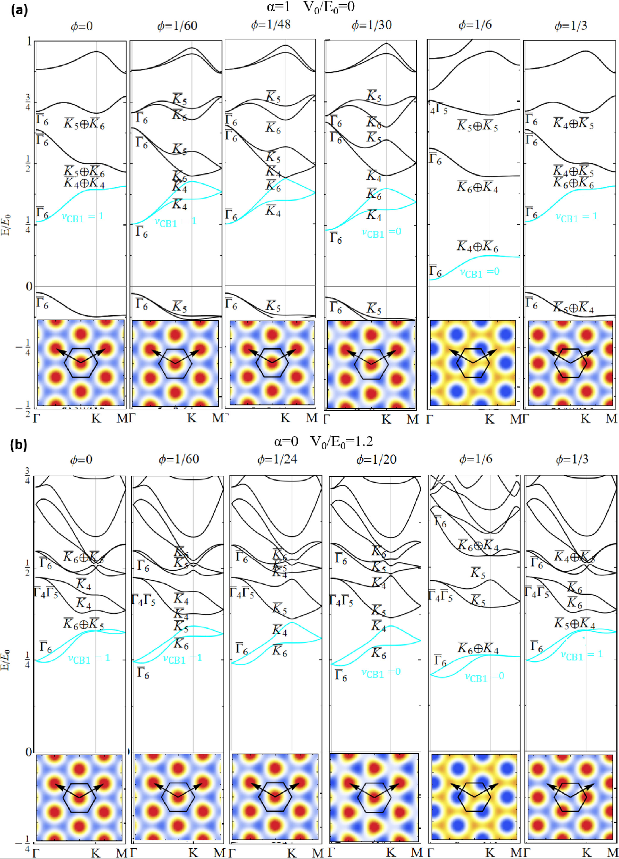
Figure S2: (a) Spectra for different $\phi$ in Fig. 2(a) of the main text. (b) Spectra for different $\phi$ in Fig. 2(b) of the main text. Insets are real space moiré potentials for different $\phi$. States are labelled with the irreducible representations by the little groups $C_{3v}$ at $\Gamma$ and $C_{3}$ at $K$. $\bar{K}_{5}$, $\bar{K}_{6}$, $\bar{K}_{4}$ represent the angular momentum states under $C_{3}$ with $J_{z}=1/2,-1/2,3/2$ respectively. $\nu$ is the $\mathbb{Z}_{2}$ invariant for the lowest conduction bands CB1.

	$\mathcal{C}_{3}$	$\mathcal{M}_{y}$	$\mathcal{T}$
$\bar{\Gamma}_{4}\bar{\Gamma}_{5}$	$\begin{pmatrix}-1&0\\ 0&-1\\ \end{pmatrix}$	$\begin{pmatrix}-i&0\\ 0&i\\ \end{pmatrix}$	$\begin{pmatrix}0&-1\\ 1&0\\ \end{pmatrix}$
$\bar{\Gamma}_{6}$	$\begin{pmatrix}e^{-i\pi/3}&0\\ 0&e^{i\pi/3}\\ \end{pmatrix}$	$\begin{pmatrix}0&-1\\ 1&0\\ \end{pmatrix}$	$\begin{pmatrix}0&1\\ -1&0\\ \end{pmatrix}$

(a) $\Gamma$

	$\mathcal{C}_{3}$
$\bar{K}_{4}$	$-1$
$\bar{K}_{5}$	$e^{-i\pi/3}$
$\bar{K}_{6}$	$e^{i\pi/3}$

(b) $K$

Table S1: (a)(b) symmetry operators in the irreducible representation at high symmetry momenta $\Gamma$ and $K$ for the double space group 156 $P3m1$ corresponding to the point group $C_{3v}$.

I.2 Topological phase transition when varying $\phi$

In this section, we study the topological phase transition of our system when varying $\phi$ of the moiré potentials. For general $\phi$, there is no inversion symmetry. As shown in Fig. S2(a), $\nu_{CB1}$ changes from $1$ to $0$ when $\phi$ varies from $0$ to $1/6$. Between the two phases, there is a gap closing around $\phi\approx 1/48$ at $K$ and $K^{\prime}$. The gap closing at $K,K^{\prime}$ happens between two states $|u_{J_{z}=-1/2}(K)\rangle$ and $|u_{J_{z}=3/2}(K)\rangle$, belonging to $\bar{K}_{6}$ and $\bar{K}_{4}$ irreducible representations as summarized in Tab.S1Xu et al. (2020); Elcoro et al. (2021), respectively, with different angular momenta $J_{z}=-1/2$ and $J_{z}=3/2$ under three-fold rotation $C_{3}$, where $|u_{J_{z}}(K)\rangle$ are eigen-states of $H_{0}(K)$ as Eq. (S44). The effective Hamiltonian on the basis $|u_{J_{z}=-1/2}(K)\rangle$ and $|u_{J_{z}=3/2}(K)\rangle$ has the Dirac fermion form $H_{eff}({\textbf{{k}}})=v_{K}(k_{x}\sigma_{x}+k_{y}\sigma_{y})+m_{K}\sigma_{z}$, up to the linear order, with $\sigma_{x,y,z}$ are Pauli matrices for the two band basis. The gap closing can be captured by one parameter, namely the Dirac mass $m_{K}$ that is controlled by $\phi$, corresponding to the co-dimension 1 case. The $\mathcal{T}$ symmetry guarantees the gap closing also occurring at $K^{\prime}$, and the gap closings at $K$ and $K^{\prime}$ lead to the change of $\mathbb{Z}_{2}$ number $\nu$ by $1$. The normal insulator (NI) states are localized at moiré potential minima of the Wyckoff position $1b$ shown by the insets of spectrum for $\phi=1/6$ in Fig. S2(a) (See SM Sec.I.D). From $\phi=1/6$ to $\phi=1/3$ in Fig. S2(a), another Dirac-type gap closing should happen at $K$ and $K^{\prime}$ , and we find the system with $\phi=1/3$ has $\nu_{\text{CB1}}=1$.

From the phase diagram in Fig. 2(a)(b) of the main text, we notice that the $\mathbb{Z}_{2}$ topological property of the system shows a periodicity when $\phi$ varies by $1/3$. Indeed, one can show that the moiré potential $\Delta(r)$ with $\phi$ and $\Delta^{\prime}(r)$ with $\phi+1/3$ (with the same $\Delta_{1}$ parameter) are related by a constant shift as

$$\begin{split}\Delta^{\prime}({\textbf{{r}}})&=\Delta_{1}e^{i2\pi\phi}e^{i2\pi/3}(e^{i{\textbf{{b}}}_{1}^{\text{M}}.{\textbf{{r}}}}+e^{i(-{\textbf{{b}}}_{1}^{\text{M}}+{\textbf{{b}}}_{2}^{\text{M}}).{\textbf{{r}}}}+e^{i(-{\textbf{{b}}}_{2}^{\text{M}}).{\textbf{{r}}}})+c.c.\\ &=\Delta_{1}e^{i2\pi\phi}(e^{i{\textbf{{b}}}_{1}^{\text{M}}.({\textbf{{r}}}+{\textbf{{a}}}_{1}^{\text{M}}/3+2{\textbf{{a}}}_{2}^{\text{M}}/3)}+e^{i(-{\textbf{{b}}}_{1}^{\text{M}}+{\textbf{{b}}}_{2}^{\text{M}}).({\textbf{{r}}}+{\textbf{{a}}}_{1}^{\text{M}}/3+2{\textbf{{a}}}_{2}^{\text{M}}/3)}+e^{i(-{\textbf{{b}}}_{2}^{\text{M}}).({\textbf{{r}}}+{\textbf{{a}}}_{1}^{\text{M}}/3+2{\textbf{{a}}}_{2}^{\text{M}}/3})+c.c.\\ &=\Delta({\textbf{{r}}}+{\textbf{{a}}}_{1}^{\text{M}}/3+2{\textbf{{a}}}_{2}^{\text{M}}/3).\end{split}$$ (S35)

As a constant shift of potential term cannot change the band topology of the system, $\nu$ must keep the same for $\phi$ and $\phi+1/3$ while keeping other parameters. For NI phase, the Wyckoff position of Wannier orbitals should also shift accordingly by ${\textbf{{a}}}_{1}^{\text{M}}/3+2{\textbf{{a}}}_{2}^{\text{M}}/3$, as shown in Fig. S7.

Similar topological phase transitions happen for $\alpha=0$ and $V_{0}/E_{0}=1.2$ by a Dirac-type gap closing at $K$ and $K^{\prime}$ between two states with different angular momenta when $\phi$ varies from $0$ to $1/6$ to $1/3$, as shown by Fig. S2(b).

The Wannier centers flows for CB1 with $\phi=0,1/6,1/3$ in Fig. S2(a) is shown in Fig. S3(a)-(c). CB1 with $\phi=0,1/3$ has nontrivial $\mathbb{Z}_{2}$ topology as analyzed in the main text. For the case with $\phi=1/6$, CB1 are topologically trivial. Similarly, the Wannier centers flows for CB1 with $\phi=0,1/6,1/3$ in Fig. S2(b) is shown in Fig. S3(d)-(f). The $\mathbb{Z}_{2}$ number of CB1 is $\nu_{CB1}=1$ for $\phi=0,1/3$ and $\nu_{CB1}=0$ for $\phi=1/6$.

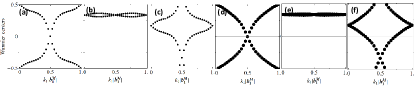
Figure S3: (a)(b)(c) The Wannier center flows for CB1 with $\phi=0,1/6,1/3$, corresponding to Fig. S2(a)(c)(d), respectively. (d)(e)(f) The Wannier center flows for CB1 with $\phi=0,1/6,1/3$, corresponding to Fig. S2(e)(g)(h), respectively.

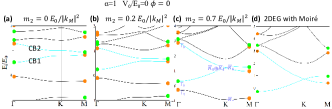
Figure S4: (a)(b)(c) Spectra with increasing $m_{2}$ for $\alpha=1,V_{0}/E_{0}=0,\phi=0$ of Fig. 2(d) in the main text. Green (Orange) dots denote even (odd) parities at $\Gamma$ and $M$. (d) Spectrum of 2DEG on the moiré potential with $\phi=0$ shown in Fig. 1(c) of the main text. Spectrum in (c) is labelled with irreps by the little group $C_{6v}$ at $\Gamma$ and $C_{3v}$ at $K$.

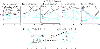
Figure S5: (a)-(e) Spectra with increasing $m_{2}$ for $\alpha=0,V_{0}/E_{0}=1.2,\phi=0$ of Fig. 2(e) in the main text. Different colorful dots $\Gamma$ represents different irreps of the little group $C_{6v}$. Spectrum in (c) is labelled with irreps by the little group $C_{6v}$ at $\Gamma$ and $C_{3v}$ at $K$. (f) spectrum around $K$ before and after breaking the inversion symmetry. $J_{z}$ is the angular momentum of the state at $K$ under $C_{3}$.

Figure S6: (a)-(f) Spectra with reducing $m_{2}$ for $\alpha=0,V_{0}/E_{0}=1.2,\phi=0$ of Fig. 2(e) in the main text. Different colorful dots $\Gamma$ represents different irreps of the little group $C_{6v}$ shown in Tab.S2. Cyan bands are CB1 and CB2. Orange ones are Cb3-5. Black ones are CB6 and higher energy bands. Insets in (d)(f) are enlargement of spectra around $\Gamma$ in the dashed boxes.

	$\mathcal{C}_{6}$	$\mathcal{M}_{y}$	$\mathcal{T}$
$\bar{\Gamma}_{7}$	$\begin{pmatrix}-i&0\\ 0&i\\ \end{pmatrix}$	$\begin{pmatrix}0&-1\\ 1&0\\ \end{pmatrix}$	$\begin{pmatrix}0&1\\ -1&0\\ \end{pmatrix}$
$\bar{\Gamma}_{8}$	$\begin{pmatrix}e^{i5\pi/6}&0\\ 0&e^{-i5\pi/6}\end{pmatrix}$	$\begin{pmatrix}0&-1\\ 1&0\\ \end{pmatrix}$	$\begin{pmatrix}0&1\\ -1&0\\ \end{pmatrix}$
$\bar{\Gamma}_{9}$	$\begin{pmatrix}e^{i\pi/6}&0\\ 0&e^{-i\pi/6}\end{pmatrix}$	$\begin{pmatrix}0&-1\\ 1&0\\ \end{pmatrix}$	$\begin{pmatrix}0&1\\ -1&0\\ \end{pmatrix}$

(a) $\Gamma$

	$\mathcal{C}_{3}$	$\mathcal{M}_{x}$
$\bar{K}_{4}$	$-1$	$-i$
$\bar{K}_{5}$	$-1$	$i$
$\bar{K}_{6}$	$\begin{pmatrix}e^{-i\pi/3}&0\\ 0&e^{i\pi/3}\end{pmatrix}$	$\begin{pmatrix}0&-1\\ 1&0\end{pmatrix}$

(b) $K$

Table S2: (a)(b) symmetry operators in the irreducible representation at high symmetry momenta $\Gamma$ and $K$ for the double space group 183 $P6mm$ corresponding to the point group $C_{6v}$.

I.3 Atomic limits at $m_{2}\rightarrow\infty$

In this section, we will provide theoretical understanding of the non-trivial morié mini-bands from the atomic limits of the CB1 and CB2 with a large $m_{2}$ term (the quadratic term of the inter-surface coupling $m$), and discuss how the realistic models with a small $m_{2}$ are connected to this atomic limit.

For $\alpha=1,V_{0}/E_{0}=0,\phi=0$ with the inversion symmetry in Fig. 2(d) of the main text, the energy spectra for increasing $m_{2}$ are shown in Fig. S4(a)-(c). We focus on CB1 and CB2 as a whole for atomic limits because they together have $\nu_{CB1}+\nu_{CB2}=0$ and are topologically trivial. When increasing $m_{2}$, we do not find any gap closing between CB1, CB2 and other valence bands or higher conduction bands. Thus, the topological properties of CB1 and CB2 remain the same, and the CB1 and CB2 are adiabatically connected to those corresponding bands in the large $m_{2}$ limit. When the $m_{2}$ term dominates in $H_{0}$, for $\phi=0$, we may consider the Hamiltonian in the $m_{z}=\pm i$ basis, Eq. (S6), and drop the linear term $\pm iv\hat{k}_{\pm}$ in the off-diagonal component first. Then, the remaining part of the Hamiltonian just describes the 2D electron gas (2DEG) with a simple parabolic dispersion on a hexagonal potential,

$$H^{\text{2DEG}}=\pm(m_{0}-m_{2}\nabla^{2})+\Delta({\textbf{{r}}}),$$ (S36)

with $\Delta({\textbf{{r}}})$ the hexagonal potential, as shown in Fig.1(c) in the main text. The corresponding conduction band dispersion with $m_{z}=-i$ is shown Fig. S4(d), while the $m_{z}=+i$ conduction bands are degenerate with $m_{z}=-i$ bands. The lowest two conduction bands of the Hamiltonian $H^{\text{2DEG}}$ can be viewed as coming from two s-wave atomic orbitals localized at the moiré hexagonal potential minima of the Wyckoff positions $1b$ and $1c$ for the point group $D_{6h}$ and give rise to a Dirac cone at K and K’, similar to the case of graphene. The off-diagonal linear term in Eq. (S6) represents the strong spin-orbit-coupling (SOC) of TI thin films, which gives rise to a small gap opening for the dispersion in Fig. S4(c) and can be treated perturbatively. We perform a ${\bf k\cdot p}$ type of perturbation expansion of the full Hamiltonian $H_{0}({\textbf{{k}}})$ around $K$. The basis wave functions are chosen to be the eigen-states of $H_{0}({\textbf{{K}}})$ in Eq. 1 of the main eigenstates without SOC ($v_{f}=0$)

$$|\tilde{u}_{J_{z},m_{z}}({\textbf{{K}}})\rangle=|\tilde{u}_{-1/2,-i}({\textbf{{K}}})\rangle,|\tilde{u}_{3/2,-i}({\textbf{{K}}})\rangle,|\tilde{u}_{3/2,i}({\textbf{{K}}})\rangle,|\tilde{u}_{+1/2,i}({\textbf{{K}}})\rangle$$ (S37)

for CB1 and CB2 with the irreps $\bar{K}_{6}$ for $|u_{1/2,+i}({\textbf{{K}}})\rangle,|u_{-1/2,-i}({\textbf{{K}}})\rangle$ and $\bar{K}_{4}$,$\bar{K}_{5}$ for $|u_{3/2,+i}({\textbf{{K}}})\rangle,|u_{3/2,-i}({\textbf{{K}}})\rangle$ (Fig. S4(c)), the detailed forms of which can be numerically evaluated. The relevant symmetry operators are

$$\mathcal{M}_{z}=-i\sigma_{z}\tau_{0}\quad\mathcal{T}\mathcal{I}=i\sigma_{y}\tau_{x}\mathcal{K}$$ (S38)

with $\sigma$ acts on the different $m_{z}$, $\tau$ acts on different $J_{z}$ in one $m_{z}$, and $\mathcal{K}$ is the complex conjugate. The SOC couples $|\tilde{u}_{J_{z},m_{z}}({\textbf{{K}}})\rangle$ and valence bands and contributes a k-independent term from the first order Löwdin perturbationWinkler (2003) by

$$H_{\text{SOC}}=C_{0}^{\prime}\sigma_{0}\tau_{0}+\Delta_{\text{KM}}\sigma_{z}\tau_{z}.$$ (S39)

The effective Hamiltonian $H_{eff}$ around $K$ to the first order in k with $m_{2}=0.7E_{0}/|k_{M}^{2}|$ is

$$H_{eff}({\textbf{{k}}})\approx H_{0}({\textbf{{K}}})+\left(\frac{\partial H_{0}({\textbf{{k}}})}{\partial{\textbf{{k}}}}\right)_{{\textbf{{k}}}={\textbf{{K}}}}\cdot{{\textbf{{k}}}}+H_{\text{SOC}}=C_{0}\sigma_{0}\tau_{0}+v_{f}(k_{x}\sigma_{0}\tau_{x}+k_{y}\sigma_{0}\tau_{y})+\Delta_{\text{KM}}\sigma_{z}\tau_{z},$$ (S40)

where $C_{0},\Delta_{\text{KM}},v_{f}$ are material dependent parameters and can be obtained numerically from the perturbation expansion. The above effective Hamiltonian $H_{eff}({\textbf{{k}}})$ resembles the Kane-Mele model Kane and Mele (2005) with the SOC term $\Delta_{\text{KM}}\sigma_{z}\tau_{z}$, which provides another understanding of the non-trivial $\mathbb{Z}_{2}$ topology of the CB1 and CB2 in our moiré system.

For $\alpha=0,V_{0}/E_{0}=1.2,\phi=0$, similar procedure can be applied to find the atomic limits of CB1 and CB2 at a large $m_{2}$. The point group in this case is $C_{6v}$ group. For $m_{2}=1.5E_{0}/|k_{M}|^{2}$ in Fig. S5(e), the effective Hamiltonian on the same basis as Eq. (S37) is given by

$$H_{eff}({\textbf{{k}}})=C_{0}\sigma_{0}\tau_{0}+v_{f}(k_{x}\sigma_{0}\tau_{x}+k_{y}\sigma_{0}\tau_{y})+\Delta_{\text{KM}}\sigma_{z}\tau_{z}+\Delta_{\text{R}}(\sigma_{x}\tau_{y}-\sigma_{y}\tau_{x}).$$ (S41)

Besides Kane-Mele SOC term $\Delta_{\text{KM}}$, there is another Rashba type of SOC term $\Delta_{\text{R}}(\sigma_{x}\tau_{y}-\sigma_{y}\tau_{x})$ as the inversion symmetry is broken for $\alpha=0$ Kane and Mele (2005). The Rashba term couples two basis functions $|\tilde{u}_{3/2,\pm i}({\textbf{{K}}})\rangle$ ($\bar{K}_{4}$ and $\bar{K}_{5}$ irreps) and opens the gap between these two states, as schematically shown in Fig. S5(f). The other two states $|\tilde{u}_{1/2,i}({\textbf{{K}}})\rangle,|\tilde{u}_{1/2,i}({\textbf{{K}}})\rangle$ ($\bar{K}_{6}$ irrep) remain degenerate and form a 2D irrep under the little group $C_{3v}$ at $K$. When this energy splitting $\Delta_{\text{R}}$ is larger than the Kane-Mele SOC gap $\Delta_{\text{KM}}$, the degenerate states with the 2D irrep $\bar{K}_{6}$ lies between the $\bar{K}_{4}$ and $\bar{K}_{5}$ state, leading to the band touching between CB1 and CB2 bands at K for $m_{2}=1.5E_{0}/|k_{M}|^{2}$ in Fig. S5(e). In this limit, the topology of the CB1 and CB2 is $\nu_{\text{CB1}}+\nu_{\text{CB2}}=0$, as the CB1 and CB2 together form an atomic limit. With decreasing $m_{2}$ to $m_{2}=0.1E_{0}/|k_{M}|^{2}$, we notice the nodes at K between CB1 and CB2 remains, but there is another band crossing between CB2 and higher conduction bands at $\Gamma$ in Fig. S5(b). This band crossing at $\Gamma$ changes the overall $\mathbb{Z}_{2}$ topology of CB1 and CB2 to $\nu_{\text{CB1}}+\nu_{\text{CB2}}=1$ for a smaller $m_{2}$. In Fig. S6, we also show the band dispersion and the irreducible representations at high symmetry momenta for other higher-energy mini-bands (labelled by CB3, CB4, CB5 and CB6). We find the mini-bands of CB3, CB4 and CB5 are always touching each other and their total $\mathbb{Z}_{2}$ number is $\nu_{\text{CB3}}+\nu_{\text{CB4}}+\nu_{\text{CB5}}=1$ for $0.04E_{0}/|k_{M}|^{2}<m_{2}<0.1E_{0}/|k_{M}|^{2}$. Another transition between CB5 and CB6 occurs at $m_{2}\approx 0.035E_{0}/|k_{M}|^{2}$ (See Fig. S6e), and after this transition, $\nu_{\text{CB3}}+\nu_{\text{CB4}}+\nu_{\text{CB5}}$ becomes zero while the other non-trivial $\mathbb{Z}_{2}$ number is moved to even higher energy mini-bands. For $m_{2}<0.1E_{0}/|k_{M}|^{2}$, these additional transitions only occur for higher-energy mini-bands, while the $\mathbb{Z}_{2}$ topology of CB1 and CB2 remains the same ($\nu_{\text{CB1}}+\nu_{\text{CB2}}=1$). For $m_{2}<0.04E_{0}/|k_{M}|^{2}$, we find a gap between CB1 and CB2 opens at K due to the interchange between the $\bar{K}_{6}$ and $\bar{K}_{5}$ mini-bands. Thus, the isolated CB1 with $\nu_{\text{CB1}}=1$ and CB2 with $\nu_{\text{CB2}}=0$ states can be found in Fig. S5(a) for $m_{2}=0$.

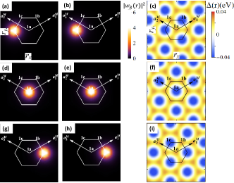
Figure S7: (a)(b) The real-space maximally localized Wannier functions $w_{\textbf{{R}}}({\textbf{{r}}})$ for the lowest conduction bands with $\phi=1/6$ corresponding to Fig. 2(a) of the main text. (c) The real space moiré potentials with $\phi=1/6$. (d)(e)(f) Those for $\phi=1/2$ and (g)(h)(i) Those for $\phi=5/6$.

I.4 Normal insulator phases of atomic limits

We construct the maximally localized Wannier functions Pizzi et al. (2020) for the topologically trivial region for the CB1 as shown in Fig. S7. The locations of Wannier functions show the NI phase of CB1 has localized orbitals at Wyckoff positions 1b for $\phi=1/6$, 1a for $\phi=1/2$, 1c for $\phi=5/6$, as indicated in the phase diagram Fig. 2(a)(b) of the main text. Comparing the Wannier functions with the moiré potentials, they are located at minima of moiré potentials and correspond to the lowest conduction bands as expected. Since the minima of potentials change from one to another when tuning $\phi$, the localized orbitals shift from one location to the other. The phase transition between two NI phases with orbitals at different Wyckoff positions has gap closingXu et al. (2021b), shown as the semi-metal phase in Fig. 2(a)(b) of the main text, as they belong to different atomic limits.

II Hartree Fock methods for Coulomb interaction

II.1 Eigenbasis projection

In this section, we project the Coulomb interaction into the eigenbasis of the non interacting Hamiltonian $H_{0}({\textbf{{k}}})$Zhang et al. (2020); Lian et al. (2021). The non-interacting moiré Hamiltonian in the second quantization form is

$$H_{0}({\textbf{{k}}})=\sum_{{\textbf{{G}}},{\textbf{{G}}}^{\prime},\alpha,\alpha^{\prime}}f_{\alpha}^{\dagger}({\textbf{{k}}}+{\textbf{{G}}})\left(H^{\text{TI}}_{\alpha,\alpha^{\prime}}({\textbf{{k}}}+{\textbf{{G}}})\delta_{{\textbf{{G}}},{\textbf{{G}}}^{\prime}}+H^{\text{M}}({\textbf{{G}}}-{\textbf{{G}}}^{\prime})\delta_{\alpha,\alpha^{\prime}}\right)f_{\alpha^{\prime}}({\textbf{{k}}}+{\textbf{{G}}}^{\prime}),$$ (S42)

where $\alpha=1,...,4$ labels both spin and layer index, $f_{\alpha}^{\dagger}({\textbf{{k}}}+{\textbf{{G}}})$ is a fermion creation operator, k is within the first moiré BZ and G is Moiré reciprocal lattice vectors. The creation operators for eigenstates of $H_{0}({\textbf{{k}}})$ are are defined as

$$c_{n}^{\dagger}({\textbf{{k}}})=\sum_{{\textbf{{G}}},\alpha}u_{{\textbf{{G}}},\alpha}^{n}({\textbf{{k}}})f_{\alpha}^{\dagger}({\textbf{{k}}}+{\textbf{{G}}}),$$ (S43)

where $u_{{\textbf{{G}}},\alpha}^{n}({\textbf{{k}}})$ satisfies the eigen equation

$$\sum_{{\textbf{{G}}}^{\prime},\alpha^{\prime}}\left({H^{\text{TI}}}_{\alpha,\alpha^{\prime}}({\textbf{{k}}}+{\textbf{{G}}})\delta_{{\textbf{{G}}},{\textbf{{G}}}^{\prime}}+H^{\text{M}}({\textbf{{G}}}-{\textbf{{G}}}^{\prime})\delta_{\alpha,\alpha^{\prime}}\right)u_{{\textbf{{G}}}^{\prime},\alpha^{\prime}}^{n}({\textbf{{k}}})=E^{n}_{0}({\textbf{{k}}})u_{{\textbf{{G}}},\alpha}^{n}({\textbf{{k}}})$$ (S44)

for $H_{0}({\textbf{{k}}})$ with energies $E_{0}^{n}({\textbf{{k}}})$. By replacing G with ${\textbf{{G}}}+{\textbf{{G}}}_{0}$ and ${\textbf{{G}}}^{\prime}$ with ${\textbf{{G}}}^{\prime}+{\textbf{{G}}}_{0}$ in Eq. (S44), we obtain

$$\sum_{{\textbf{{G}}}^{\prime},\alpha^{\prime}}\left({H^{\text{TI}}}_{\alpha,\alpha^{\prime}}({\textbf{{k}}}+{\textbf{{G}}}_{0}+{\textbf{{G}}})\delta_{{\textbf{{G}}},{\textbf{{G}}}^{\prime}}+H^{\text{M}}({\textbf{{G}}}-{\textbf{{G}}}^{\prime})\delta_{\alpha,\alpha^{\prime}}\right)u_{{\textbf{{G}}}^{\prime}+{\textbf{{G}}}_{0},\alpha^{\prime}}^{n}({\textbf{{k}}})=E^{n}_{0}({\textbf{{k}}})u_{{\textbf{{G}}}+{\textbf{{G}}}_{0},\alpha}^{n}({\textbf{{k}}}),$$ (S45)

which can be viewed as the eigen equations for $u_{{\textbf{{G}}},\alpha}^{n}({\textbf{{k}}}+{\textbf{{G}}}_{0})$ by replacing k with ${\textbf{{k}}}+{\textbf{{G}}}_{0}$ in Eq. (S44),

$$\sum_{{\textbf{{G}}}^{\prime},\alpha^{\prime}}\left({H^{\text{TI}}}_{\alpha,\alpha^{\prime}}({\textbf{{k}}}+{\textbf{{G}}}_{0}+{\textbf{{G}}})\delta_{{\textbf{{G}}},{\textbf{{G}}}^{\prime}}+H^{\text{M}}({\textbf{{G}}}-{\textbf{{G}}}^{\prime})\delta_{\alpha,\alpha^{\prime}}\right)u_{{\textbf{{G}}}^{\prime},\alpha^{\prime}}^{n}({\textbf{{k}}}+{\textbf{{G}}}_{0})=E^{n}_{0}({\textbf{{k}}}+{\textbf{{G}}}_{0})u_{{\textbf{{G}}},\alpha}^{n}({\textbf{{k}}}+{\textbf{{G}}}_{0}).$$ (S46)

Thus, we can fix the periodic gauge for the eigen-state as

$$u_{{\textbf{{G}}}+{\textbf{{G}}}_{0},\alpha}^{n}({\textbf{{k}}})=u_{{\textbf{{G}}},\alpha}^{n}({\textbf{{k}}}+{\textbf{{G}}}_{0}).$$ (S47)

As $u_{G,\alpha}^{n}({\textbf{{k}}})$ is a set of orthonormal basis, we can take the inverse of the above expansion as

$$f_{\alpha}^{\dagger}({\textbf{{k}}}+{\textbf{{G}}})=\sum_{n}u_{{\textbf{{G}}},\alpha}^{n*}({\textbf{{k}}})c_{n}^{\dagger}({\textbf{{k}}})$$ (S48)

and

$$\left\{c_{n}({\textbf{{k}}}),c_{n^{\prime}}^{\dagger}({\textbf{{k}}}^{\prime})\right\}=\sum_{{\textbf{{G}}},\alpha}u_{G,\alpha}^{n*}({\textbf{{k}}})\sum_{{\textbf{{G}}}^{\prime},\alpha^{\prime}}u_{{\textbf{{G}}}^{\prime},\alpha^{\prime}}^{n^{\prime}}({\textbf{{k}}}^{\prime})\left\{f_{\alpha}({\textbf{{k}}}+{\textbf{{G}}}),f_{\alpha^{\prime}}^{\dagger}({\textbf{{k}}}^{\prime}+{\textbf{{G}}}^{\prime})\right\}=\delta_{n,n^{\prime}}\delta({\textbf{{k}}}-{\textbf{{k}}}^{\prime}).$$ (S49)

To improve the efficiency of the numerical calculations, we need to further fix the gauge freedom of eigenstates. An important step is to choose the real gauge for the Hamiltonian and eigenbasis due to the space-time inversion symmetry $C_{2z}\mathcal{T}$ in 2D for moiré potential with $\phi=0$. Take $C_{2z}\mathcal{T}=U_{\text{CT}}\mathcal{K}$ with $\mathcal{K}$ as complex conjugate. $U_{\text{CT}}$ is unitary and satisfies the $U_{\text{CT}}{}^{*}U_{\text{CT}}=1$ from $\left(C_{2z}\mathcal{T}\right){}^{2}=1$. Under the basis transformation $U_{\text{CT}}{}^{1/2}$,

$$\left(U_{\text{CT}}{}^{1/2}\right){}^{\dagger}C_{2z}\mathcal{T}U_{\text{CT}}{}^{1/2}=U_{\text{CT}}{}^{-1/2}U_{\text{CT}}\left(U_{\text{CT}}{}^{1/2}\right){}^{*}\mathcal{K}=\mathcal{K},$$ (S50)

and the corresponding Hamiltonian and eigenbasis can be chosen to be real. There is still a $SO(2)$ gauge freedom left for eigenstates for Fig. 2(d) in the main text with inversion and $\pm$ gauge freedom for Fig. 2(e) in the main text without inversion.

In the eigenbasis, the non-interacting Hamiltonian is

$$H_{0}({\textbf{{k}}})=\sum_{n}c_{n}^{\dagger}({\textbf{{k}}})E_{0}^{n}(k)c_{n}({\textbf{{k}}}).$$ (S51)

The dual-gated Coulomb interaction potential is Zhang et al. (2020); Bernevig et al. (2021)

$$V({\textbf{{q}}})=\frac{e^{2}\tanh|{\textbf{{q}}}|d}{2\epsilon_{0}\epsilon_{r}|{\textbf{{q}}}|}\frac{1}{S},$$ (S52)

where $S$ is the area, $d$ is the dual-gate distance, $\epsilon_{0}\epsilon_{r}$ are permittivity, $e$ is electron charge. The Coulomb interaction Hamiltonian in second quantization form is

$$\begin{split}H_{\text{I}}&=\frac{1}{2}\sum_{{\textbf{{k}}}_{1},{\textbf{{k}}}_{2},{\textbf{{q}}},{\textbf{{G}}}}\sum_{{\textbf{{G}}}_{1},\alpha_{1},{\textbf{{G}}}_{2},\alpha_{2}}V({\textbf{{q}}}+{\textbf{{G}}})\\ &f_{\alpha_{1}}^{\dagger}\left({\textbf{{k}}}_{1}+{\textbf{{G}}}_{1}+{\textbf{{q}}}+{\textbf{{G}}}\right)f_{\alpha_{2}}^{\dagger}\left({\textbf{{k}}}_{2}+{\textbf{{G}}}_{2}-{\textbf{{q}}}-{\textbf{{G}}}\right)f_{\alpha_{2}}\left({\textbf{{k}}}_{2}+{\textbf{{G}}}_{2}\right)f_{\alpha_{1}}\left({\textbf{{k}}}_{1}+{\textbf{{G}}}_{1}\right)\\ &=\frac{1}{2}\sum_{{\textbf{{k}}}_{1},{\textbf{{k}}}_{2},{\textbf{{q}}},{\textbf{{G}}}}\sum_{m_{1},n_{1},m_{2},n_{2}}V({\textbf{{q}}}+{\textbf{{G}}})\Lambda_{m_{1}n_{1}}\left({\textbf{{k}}}_{1}+{\textbf{{q}}}+{\textbf{{G}}},{\textbf{{k}}}_{1}\right)\Lambda_{m_{2}n_{2}}\left({\textbf{{k}}}_{2}-{\textbf{{q}}}-{\textbf{{G}}},{\textbf{{k}}}_{2}\right)\\ &c_{m_{1}}^{\dagger}\left({\textbf{{k}}}_{1}+{\textbf{{q}}}\right)c_{m_{2}}^{\dagger}\left({\textbf{{k}}}_{2}-{\textbf{{q}}}\right)c_{n_{2}}\left({\textbf{{k}}}_{2}\right)c_{n_{1}}\left({\textbf{{k}}}_{1}\right)\end{split}$$ (S53)

with the form factor

$$\Lambda_{m_{1}n_{1}}\left({\textbf{{k}}}_{1}+{\textbf{{G}}},{\textbf{{k}}}_{2}\right)=\sum_{{\textbf{{G}}}^{\prime},\alpha^{\prime}}u_{{\textbf{{G}}}^{\prime},\alpha^{\prime}}^{m_{1}*}\left({\textbf{{k}}}_{1}+{\textbf{{G}}}\right)u_{{\textbf{{G}}}^{\prime},\alpha^{\prime}}^{n_{1}}\left({\textbf{{k}}}_{2}\right)=\left\langle u^{m_{1}}\left({\textbf{{k}}}_{1}+{\textbf{{G}}}\right)|u^{n_{1}}\left({\textbf{{k}}}_{2}\right)\right\rangle.$$ (S54)

The form factor satisfies

$$\Lambda_{m_{1}n_{1}}\left({\textbf{{k}}}_{1}+{\textbf{{G}}},{\textbf{{k}}}_{2}\right)=\Lambda_{n_{1}m_{1}}^{*}\left({\textbf{{k}}}_{2},{\textbf{{k}}}_{1}+{\textbf{{G}}}\right)=\Lambda_{m_{1}n_{1}}\left({\textbf{{k}}}_{1},{\textbf{{k}}}_{2}-{\textbf{{G}}}\right).$$ (S55)

In the real eigenbasis, the form factors are all real.

II.2 Self-consistent Hartree-Fock mean field Theory

In this section, we treat the Coulomb interaction under the Hartree-Fock (HF) approximationZhang et al. (2020). The basic idea is the decoupling of four-fermion operators by

$$\begin{split}c_{1}^{\dagger}c_{1}c_{2}^{\dagger}c_{2}&=\left(\left\langle c_{1}^{\dagger}c_{1}\right\rangle+c_{1}^{\dagger}c_{1}-\left\langle c_{1}^{\dagger}c_{1}\right\rangle\right)\left(\left\langle c_{2}^{\dagger}c_{2}\right\rangle+c_{2}^{\dagger}c_{2}-\left\langle c_{2}^{\dagger}c_{2}\right\rangle\right)\\ &\approx\left\langle c_{1}^{\dagger}c_{1}\right\rangle\left\langle c_{2}^{\dagger}c_{2}\right\rangle+\left\langle c_{1}^{\dagger}c_{1}\right\rangle\left(c_{2}^{\dagger}c_{2}-\left\langle c_{2}^{\dagger}c_{2}\right\rangle\right)+\left(c_{1}^{\dagger}c_{1}-\left\langle c_{1}^{\dagger}c_{1}\right\rangle\right)\left\langle c_{2}^{\dagger}c_{2}\right\rangle\\ &=\left\langle c_{1}^{\dagger}c_{1}\right\rangle c_{2}^{\dagger}c_{2}+c_{1}^{\dagger}c_{1}\left\langle c_{2}^{\dagger}c_{2}\right\rangle-\left\langle c_{1}^{\dagger}c_{1}\right\rangle\left\langle c_{2}^{\dagger}c_{2}\right\rangle.\end{split}$$ (S56)

The expectation value of the two-fermion operator is the density matrix

$$\rho_{mn}({\textbf{{k}}})=\left\langle c_{m}^{\dagger}({\textbf{{k}}})c_{n}({\textbf{{k}}})\right\rangle=\sum_{j}\psi^{\text{HF *}}_{j,m}({\textbf{{k}}})\psi^{\text{HF}}_{j,n}({\textbf{{k}}})n_{F}\left(E_{j}^{\text{HF}}({\textbf{{k}}})\right)$$ (S57)

determined by with $n_{F}$ as the Fermi distribution function and $\psi^{\text{HF}}_{j,m}({\textbf{{k}}})$,$E_{j}^{\text{HF}}({\textbf{{k}}})$ as the $j$-th eigenstates and eigen-energies of Hartree-Fock Hamiltonian

$$\sum_{m}H^{\text{HF}}_{nm}[\rho]({\textbf{{k}}})\psi^{\text{HF}}_{j,m}({\textbf{{k}}})=E_{j}^{\text{HF}}({\textbf{{k}}})\psi^{\text{HF}}_{j,n}({\textbf{{k}}}),$$ (S58)

where $H^{\text{HF}}_{nm}[\rho]({\textbf{{k}}})$ is defined in Eq. Eq. (S61) below. We always choose $E_{j=1}^{\text{HF}}({\textbf{{k}}})<E_{j=2}^{\text{HF}}({\textbf{{k}}})<....$, so the mean field ground state is given by the eigen-state $\psi^{\text{HF}}_{j=1}({\textbf{{k}}})$. Here, we do not consider non-uniform order parameters in real space with the form $\left\langle c_{m}^{\dagger}({\textbf{{k}}})c_{n}({\textbf{{k}}}+{\textbf{{q}}})\right\rangle$ for ${\textbf{{q}}}\neq 0$.

The Coulomb interaction under Hartree-Fock approximation is

$$\begin{split}H_{\text{I}}[\rho({\textbf{{k}}})]&=\frac{1}{2}\sum_{{\textbf{{k}}}_{1},{\textbf{{k}}}_{2},{\textbf{{q}}},{\textbf{{G}}}}V({\textbf{{q}}}+{\textbf{{G}}})\sum_{m_{1},n_{1},m_{2},n_{2}}\Lambda_{m_{1}n_{1}}\left({\textbf{{k}}}_{1}+{\textbf{{q}}}+{\textbf{{G}}},{\textbf{{k}}}_{1}\right)\Lambda_{m_{2}n_{2}}\left({\textbf{{k}}}_{2}-{\textbf{{q}}}-{\textbf{{G}}},{\textbf{{k}}}_{2}\right)\\ &\quad(\delta_{{\textbf{{q}}}=0}\left(\rho_{m_{1}n_{1}}\left({\textbf{{k}}}_{1}\right)c_{m_{2}}^{\dagger}\left({\textbf{{k}}}_{2}\right)c_{n_{2}}\left({\textbf{{k}}}_{2}\right)+c_{m_{1}}^{\dagger}\left({\textbf{{k}}}_{1}\right)c_{n_{1}}\left({\textbf{{k}}}_{1}\right)\rho_{m_{2}n_{2}}\left({\textbf{{k}}}_{2}\right)-\rho_{m_{1}n_{1}}\left({\textbf{{k}}}_{1}\right)\rho_{m_{2}n_{2}}\left({\textbf{{k}}}_{2}\right)\right)\\ &-\delta_{{\textbf{{q}}}={\textbf{{k}}}_{2}-{\textbf{{k}}}_{1}}\left(\rho_{m_{1}n_{2}}\left({\textbf{{k}}}_{2}\right)c_{m_{2}}^{\dagger}\left({\textbf{{k}}}_{1}\right)c_{n_{1}}\left({\textbf{{k}}}_{1}\right)+c_{m_{1}}^{\dagger}\left({\textbf{{k}}}_{2}\right)c_{n_{2}}\left({\textbf{{k}}}_{2}\right)\rho_{m_{2}n_{1}}\left({\textbf{{k}}}_{1}\right)-\rho_{m_{1}n_{2}}\left({\textbf{{k}}}_{2}\right)\rho_{m_{2}n_{1}}\left({\textbf{{k}}}_{1}\right)\right))\\ &=\sum_{{\textbf{{k}}}_{1}}C^{\dagger}\left({\textbf{{k}}}_{1}\right)\left(H_{\text{I}}^{\text{H}}[\rho]\left({\textbf{{k}}}_{1}\right)-H_{\text{I}}^{\text{F}}[\rho]\left({\textbf{{k}}}_{1}\right)\right)C\left({\textbf{{k}}}_{1}\right)-E_{C}[\rho].\end{split}$$ (S59)

with the Hartree term $H_{\text{I}}^{\text{H}}[\rho]\left({\textbf{{k}}}_{1}\right)$, Fock term $H_{\text{I}}^{\text{F}}[\rho]\left({\textbf{{k}}}_{1}\right)$, condensation energy $E_{C}[\rho]$ defined as

$$\begin{split}H_{\text{I}}^{\text{H}}[\rho]\left({\textbf{{k}}}_{1}\right)&=\sum_{{\textbf{{k}}}_{2},{\textbf{{G}}}}V({\textbf{{G}}})\Lambda\left({\textbf{{k}}}_{1}-{\textbf{{G}}},{\textbf{{k}}}_{1}\right)\text{Tr}\left(\rho\left({\textbf{{k}}}_{2}\right)\Lambda^{*}\left({\textbf{{k}}}_{2}-{\textbf{{G}}},{\textbf{{k}}}_{2}\right)\right)\\ H_{\text{I}}^{\text{F}}[\rho]\left({\textbf{{k}}}_{1}\right)&=\sum_{{\textbf{{k}}}_{2},{\textbf{{G}}}}V\left({\textbf{{k}}}_{2}-{\textbf{{k}}}_{1}+{\textbf{{G}}}\right)\Lambda\left({\textbf{{k}}}_{1}-{\textbf{{G}}},{\textbf{{k}}}_{2}\right)\rho^{T}\left({\textbf{{k}}}_{2}\right)\Lambda^{\dagger}\left({\textbf{{k}}}_{1}-{\textbf{{G}}},{\textbf{{k}}}_{2}\right)\\ E_{C}[\rho]&=\frac{1}{2}\sum_{{\textbf{{k}}}_{1},{\textbf{{k}}}_{2},{\textbf{{G}}}}V({\textbf{{G}}})\text{Tr}\left(\rho\left({\textbf{{k}}}_{1}\right)\Lambda^{T}\left({\textbf{{k}}}_{1}-{\textbf{{G}}},{\textbf{{k}}}_{1}\right)\right)\text{Tr}\left(\rho\left({\textbf{{k}}}_{2}\right)\Lambda^{*}\left({\textbf{{k}}}_{2}-{\textbf{{G}}},{\textbf{{k}}}_{2}\right)\right)\\ &-\frac{1}{2}\sum_{{\textbf{{k}}}_{1},{\textbf{{k}}}_{2},{\textbf{{G}}}}V\left({\textbf{{k}}}_{2}-{\textbf{{k}}}_{1}+{\textbf{{G}}}\right)\text{Tr}\left(\rho^{T}\left({\textbf{{k}}}_{1}\right)\Lambda\left({\textbf{{k}}}_{1}-{\textbf{{G}}},{\textbf{{k}}}_{2}\right)\rho^{T}\left({\textbf{{k}}}_{2}\right)\Lambda^{\dagger}\left({\textbf{{k}}}_{1}-{\textbf{{G}}},{\textbf{{k}}}_{2}\right)\right).\\ \end{split}$$ (S60)

$C^{\dagger}(k)=(c_{1}^{\dagger}({\textbf{{k}}}),c_{2}^{\dagger}({\textbf{{k}}})),\dots,c_{n}^{\dagger}({\textbf{{k}}}))$ with $n$ as the number of bands projected. Since the $H_{0}({\textbf{{k}}})$ comes from DFT with Hartree-Fock interaction, the non-interacting states $\psi^{\text{HF}}_{j,m}(k)=\delta_{j,m}$ or $\rho_{0}({\textbf{{k}}})$ would be a solution to the Hartree-Fock mean-field Hamiltonian. To achieve this, the $H_{\text{I}}\left[\rho_{0}\right]$ is subtracted from $H_{\text{I}}\left[\rho\right]$ Zhang et al. (2020); Liu et al. (2021). We define the Hartree-Fock Hamiltonian to be

$$\begin{split}H^{\text{HF}}[\rho]({\textbf{{k}}})&=H_{0}({\textbf{{k}}})+H^{\text{H}}_{\text{I}}[\rho]({\textbf{{k}}})-H^{\text{F}}_{\text{I}}[\rho]({\textbf{{k}}})-\left(H^{\text{H}}_{\text{I}}\left[\rho_{0}\right]({\textbf{{k}}})-H^{\text{F}}_{\text{I}}[\rho_{0}]({\textbf{{k}}})\right)\\ &=H_{0}({\textbf{{k}}})+H^{\text{H}}_{\text{I}}[\rho-\rho_{0}]({\textbf{{k}}})-H^{\text{F}}_{\text{I}}[\rho-\rho_{0}]({\textbf{{k}}}).\end{split}$$ (S61)

We solve $H^{\text{HF}}[\rho]({\textbf{{k}}})$ self-consistently in the following standard procedures. We first choose an initial guess of the density matrix, denoted as $\rho_{ini}({\textbf{{k}}})$, as the order parameter for the filling of one band (half filling in two-band model and one quarter filling for four-band model). Based on $\rho_{ini}({\textbf{{k}}})$, we can construct $H^{\text{HF}}[\rho_{ini}]({\textbf{{k}}})$ from Eq. (S61) and calculate the corresponding new eigenstates that allow us to construct the new density matrix, denoted as $\rho_{new}({\textbf{{k}}})$. We reset $\rho_{ini}({\textbf{{k}}})=\rho_{new}({\textbf{{k}}})$ and continue the iterative process until the convergence is achieved. The criterion for the convergence is taken as the spectra $\tilde{E}_{j}^{\text{HF}}({\textbf{{k}}})$ of $H^{\text{HF}}[\rho_{ini}]$ and $E_{j}^{\text{HF}}({\textbf{{k}}})$ of $H^{\text{HF}}[\rho_{new}]$ satisfy

$$\max_{j,{\textbf{{k}}}}|\tilde{E}_{j}^{\text{HF}}({\textbf{{k}}})-E_{j}^{\text{HF}}({\textbf{{k}}})|<10^{-5}E_{0}$$ (S62)

with $\max$ taken for all bands $j$ in $H^{\text{HF}}$ and k on the high symmetry lines $\Gamma-K-M$ as shown in Fig. S8(a). $E_{0}=v|{\textbf{{b}}}_{1}^{\text{M}}|$.

The final self-consistent solution for the density matrix is denoted as $\rho^{HF}({\textbf{{k}}})$ which is determined by the eigen wavefunctions $|\psi^{\text{HF}}_{j}({\textbf{{k}}})\rangle$ by Eq. (S57) and (S58). The energy per particles for each self-consistent solution to the mean-field Hamiltonian is

$$E_{\text{I}}[\rho]=\frac{1}{N}\sum_{\textbf{{k}}}\text{Tr$\rho$}^{T}({\textbf{{k}}})H^{\text{HF}}[\rho]({\textbf{{k}}})-\left(E_{C}[\rho]-E_{C}\left[\rho_{0}\right]\right).$$ (S63)

with $N$ as the number of electrons for the filling.

II.3 Two-band model of CB1

In this section, we discuss the self-consistent solutions of $H^{\text{HF}}({\textbf{{k}}})$ at half filling of two-band model for CB1. Below we will discuss both the inversion-symmetric and asymmetric cases.

We first describe our gauge choice of the non-interacting eigen-states for the case $\alpha=1,V_{0}/E_{0}=0,\phi=0$ with inversion symmetry, which is important to simplify the numerical calculations. The non-interacting states are $|u^{\text{CB1}}_{\pm i}({\textbf{{k}}})\rangle$ with the $m_{z}$ eigenvalues $\pm i$. The mirror Chern numberFu (2011) $C=\pm 1$ can be defined for $|u^{\text{CB1}}_{\pm i}({\textbf{{k}}})\rangle$. $C_{2z}\mathcal{T}$ relates two $m_{z}$-eigen states by

$$C_{2z}\mathcal{T}|u^{\text{CB1}}_{\pm i}({\textbf{{k}}})\rangle=|u^{\text{CB1}}_{\mp i}({\textbf{{k}}})\rangle.$$ (S64)

It turns out that the Hartree-Fock calculations can be simplified by taking the real gauge due to the $C_{2z}\mathcal{T}$ symmetry and thus we transform the basis wavefunctions into the real-gauge form

$$\begin{split}|u^{\text{R},\text{CB1}}_{+}({\textbf{{k}}})\rangle=\frac{1}{\sqrt{2}}\left(e^{\text{i$\varphi$}_{\textbf{{k}}}}|u^{\text{CB1}}_{-i}({\textbf{{k}}})\rangle+e^{-\text{i$\varphi$}_{\textbf{{k}}}}|u^{\text{CB1}}_{+i}({\textbf{{k}}})\rangle\right)\\ |u^{\text{R},\text{CB1}}_{-}({\textbf{{k}}})\rangle=\frac{1}{\sqrt{2}i}\left(e^{\text{i$\varphi$}_{\textbf{{k}}}}|u^{\text{CB1}}_{-i}({\textbf{{k}}})\rangle-e^{-\text{i$\varphi$}_{\textbf{{k}}}}|u^{\text{CB1}}_{+i}({\textbf{{k}}})\rangle\right),\end{split}$$ (S65)

where $\varphi_{k}$ is the remaining relative $U(1)$ phase between eigen-states opposite $m_{z}$ (spin $U(1)$ symmetry). The real eigen-states with different $\varphi_{k}$ can be related by a $SO(2)$ transformation

$$R(\tilde{\varphi}_{\textbf{{k}}})=\begin{pmatrix}\cos\tilde{\varphi}_{\textbf{{k}}}&-\sin\tilde{\varphi}_{\textbf{{k}}}\\ \sin\tilde{\varphi}_{\textbf{{k}}}&\cos\tilde{\varphi}_{\textbf{{k}}}\\ \end{pmatrix},$$ (S66)

which shifts $\varphi_{\textbf{{k}}}$ to $\varphi_{\textbf{{k}}}+\tilde{\varphi}_{\textbf{{k}}}$. The other symmetry operators can be taken as

$$\mathcal{T}=i\sigma_{y}\mathcal{K};\quad C_{2z}=-i\sigma_{y};\quad C_{2z}\mathcal{T}=\mathcal{K};\quad\mathcal{M}_{z}=-i\sigma_{y},$$ (S67)

with Pauli matrices $\sigma$ redefined under the basis $|u^{\text{R},\text{CB1}}_{\pm}({\textbf{{k}}})\rangle$. $|u^{\text{R},\text{CB1}}_{\pm}({\textbf{{k}}})\rangle$ are taken as the eigenstates projected for the self-consistent Hartree-Fock calculations, which are related to the basis $|u^{\text{CB1}}_{m_{z}=\pm i}\rangle$ used in the main text by Eq. (S65). The density matrices in the main text, denoted as $[\rho]_{\alpha\beta}=\langle u^{\text{CB1}}_{\alpha}|\hat{\rho}|u^{\text{CB1}}_{\beta}\rangle$ with $\alpha,\beta=\pm i$, are related to the density matrices $\rho^{\text{R}}$ in the real basis discussed below, denoted as $[\rho^{\text{R}}]_{\alpha\beta}=\langle u^{\text{R,CB1}}_{\alpha}|\hat{\rho}|u^{\text{R, CB1}}_{\beta}\rangle$ with $\alpha,\beta=\pm$, by

$$\rho^{\text{R}}=U^{\text{R}\dagger}\rho U^{\text{R}}$$ (S68)

and

$$U^{\text{R}}({\textbf{{k}}})=\frac{1}{\sqrt{2}}\begin{pmatrix}e^{i\varphi_{\textbf{{k}}}}&-ie^{i\varphi_{\textbf{{k}}}}\\ e^{-i\varphi_{\textbf{{k}}}}&ie^{-i\varphi_{\textbf{{k}}}}\\ \end{pmatrix},$$ (S69)

which transforms Pauli matrices $\sigma$ as $U^{\text{R}\dagger}\sigma_{y}U^{\text{R}}=\sigma_{x}\cos{2\varphi_{\textbf{{k}}}}-\sigma_{z}\sin{2\varphi_{\textbf{{k}}}},U^{\text{R}\dagger}\sigma_{x}U^{\text{R}}=\sigma_{x}\sin{2\varphi_{\textbf{{k}}}}+\sigma_{z}\cos{2\varphi_{\textbf{{k}}}},U^{\text{R}\dagger}\sigma_{z}U^{\text{R}}=\sigma_{y}$.

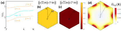
Figure S8: (a) The spectrum of $H^{\text{HF}}({\textbf{{k}}})$ for mirror polarized states with $\rho^{\text{R}}_{y}({\textbf{{k}}})$ (orange lines) . (b)(c) The overlap between Hartree-Fock states $|\psi^{\text{H}F}_{j=1}({\textbf{{k}}})\rangle$ in (a) and the non-interacting mirror polarized basis wavefunction $|u^{\text{CB1}}_{\pm i}\rangle({\textbf{{k}}})$. (d) The Berry curvature $\Omega_{xy}({\textbf{{k}}})$ over the moiré BZ for the filled band. Here the calculation is for the two-band model with the parameters $\phi=0,\alpha=1,V_{0}/E_{0}=0$.

We performed the self-consistent calculations on the basis $|u^{\text{R},\text{CB1}}_{\pm}({\textbf{{k}}})\rangle$ and generally consider the following two types of order parameters: $\rho^{\text{R}}_{y}({\textbf{{k}}})=f_{0y}({\textbf{{k}}})\sigma_{0}+f_{y}({\textbf{{k}}})\sigma_{y}$ and $\rho^{\text{R}}_{zx}({\textbf{{k}}})=f_{0zx}({\textbf{{k}}})\sigma_{0}+f_{x}({\textbf{{k}}})\sigma_{x}+f_{z}({\textbf{{k}}})\sigma_{z}$ with $\sigma$ acting on the basis $|u^{\text{R},\text{CB1}}_{\pm}({\textbf{{k}}})\rangle$ in Eq. (S65). These two types of order parameters possess different symmetry properties as summarized in Tab.S3. For $\rho^{\text{R}}_{y}({\textbf{{k}}})$, the density matrix breaks the $C_{2z}\mathcal{T}$ symmetry with complex $f_{y}({\textbf{{k}}})\sigma_{y}$ and preserves $SO(2)$ symmetry in Eq. (S66) by $[R(\tilde{\varphi}_{\textbf{{k}}}),\rho^{\text{R}}_{y}({\textbf{{k}}})]=0$. $\rho^{\text{R}}_{y}({\textbf{{k}}})$ also preserves the z-directional mirror symmetry, $[\rho^{\text{R}}_{y}({\textbf{{k}}}),\mathcal{M}_{z}]=0$, as $\mathcal{M}_{z}=-i\sigma_{y}$ in the $|u^{\text{R},\text{CB1}}_{\pm}({\textbf{{k}}})\rangle$ basis, which is the generator of the $SO(2)$ symmetry. It represents the many-body states polarized to one of the mirror states $|u^{\text{CB1}}_{m_{z}}\rangle$, dubbed as mirror-polarized states. For $\rho^{\text{R}}_{zx}({\textbf{{k}}})$, the density matrix is real and preserves the $C_{2z}\mathcal{T}$ symmetry ($[C_{2z}\mathcal{T},\rho^{\text{R}}_{zx}({\textbf{{k}}})]=0$) but breaks $SO(2)$ symmetry. It represents the many-body states with superposition of both mirror states $|u^{\text{CB1}}_{m_{z}}\rangle$, dubbed as mirror-coherent states. The identity matrix $\sigma_{0}$ appears in both order parameters and mainly determines the filling of states $|\psi^{\text{HF}}_{j}({\textbf{{k}}})\rangle$ at different momenta k.

	$\mathcal{T}$	$C_{2z}$	$C_{2z}\mathcal{T}$	$\mathcal{M}_{z}$	$\mathcal{I}$	$C_{6z}$	$C_{3z}$	$\mathcal{M}_{x}$	$\mathcal{M}_{y}$
	$i\tau_{0}s_{y}\mathcal{K}$	$-i\tau_{0}s_{z}$	$i\tau_{0}s_{x}\mathcal{K}$	$-i\tau_{x}s_{z}$	$\tau_{x}s_{0}$	$\exp(-i\pi\tau_{0}s_{z}/6)$	$\exp(-i\pi\tau_{0}s_{z}/3)$	$-i\tau_{0}s_{x}$	$-i\tau_{0}s_{y}$
	$i\sigma_{y}\mathcal{K}$	$-i\sigma_{y}$	$\mathcal{K}$	$-i\sigma_{y}$	$\sigma_{0}$	$\exp(-i\pi\sigma_{y}/6)$	$\exp(-i\pi\sigma_{y}/3)$	$-i\sigma_{z}$	$-i\sigma_{x}$
$\rho_{y}^{\text{R,HF}}({\textbf{{k}}})$	$\times$	✓	$\times$	✓	✓	✓	✓	$\times$	$\times$
$\rho_{zx}^{\text{R,HF}}({\textbf{{k}}})$	$\times$	$\times$	✓	$\times$	✓	$\times$	$\times$	✓	$\times$

Table S3: A summary of symmetries preserved (✓) or broken ($\times$) by the mirror polarized states with $\rho_{y}^{\text{R,HF}}({\textbf{{k}}})$ and the mirror coherent states with $\rho_{zx}^{\text{R,HF}}({\textbf{{k}}})$. $\rho^{\text{R,HF}}({\textbf{{k}}})$ are the self-consistent solutions from the mean-field Hamiltonian $H^{\text{HF}}({\textbf{{k}}})$. The symmetry operators are written in two basis. $\tau,s$ are Pauli matrices for the surface and spin basis as Eq.1 in the main text. $\sigma$ are the Pauli matrices for the real basis $|u^{\text{R,CB1}}_{\pm}({\textbf{{k}}})\rangle$.

Different symmetry properties of $\rho^{\text{R}}_{y}({\textbf{{k}}})$ and $\rho^{\text{R}}_{zx}({\textbf{{k}}})$ under the $C_{2z}\mathcal{T}$ and $SO(2)$ symmetry guarantee that they will not mix with each other. We may start from the initial density matrix $\rho^{\text{R}}_{ini}({\textbf{{k}}})=\rho^{\text{R}}_{y}({\textbf{{k}}})$ with certain forms of $f_{0y}$ and $f_{y}$, which preserves the $R(\tilde{\varphi}_{\textbf{{k}}})$ symmetry, $[\rho^{\text{R}}_{ini}({\textbf{{k}}}),R(\tilde{\varphi}_{\textbf{{k}}})]=0$. As the Hartree-Fock Hamiltonian $H^{\text{HF}}[\rho^{\text{R}}_{ini}]({\textbf{{k}}})$ is constructed from $\rho^{\text{R}}_{ini}$, direct calculation shows that $[H^{\text{HF}}[\rho^{\text{R}}_{ini}]({\textbf{{k}}}),R(\tilde{\varphi}_{\textbf{{k}}})]=0$ for any $\varphi_{\textbf{{k}}}$. From Eq. (S66) of $R(\tilde{\varphi}_{\textbf{{k}}})$, the Hamiltonian has to take the form

$$H^{\text{HF}}[\rho^{\text{R}}_{ini}]({\textbf{{k}}})=h_{0}({\textbf{{k}}})\sigma_{0}+h_{y}({\textbf{{k}}})\sigma_{y},$$ (S70)

where $h_{0}({\textbf{{k}}}),h_{y}({\textbf{{k}}})$ are some functions of k which can be determined numerically. From the above form of the Hamiltonian, the new density matrix can be evaluated as

$$\rho^{\text{R}}_{new}({\textbf{{k}}})=\sum_{j=\pm}n_{F}\left(h_{0}({\textbf{{k}}})+jh_{y}({\textbf{{k}}})\right)\frac{1}{2}\left(\sigma_{0}-j\sigma_{y}\right),$$ (S71)

which still satisfies $[\rho^{\text{R}}_{new}({\textbf{{k}}}),R(\tilde{\varphi}_{\textbf{{k}}})]=0$. $n_{F}(E)$ is the Fermi distribution function. Thus, the $R(\tilde{\varphi}_{\textbf{{k}}})$ symmetry is preserved in the self-consistent calculation process and thus the Pauli matrices $\sigma_{x}$ and $\sigma_{z}$ cannot be generated in the final $\rho^{\text{R,HF}}_{y}({\textbf{{k}}})$.

Similar argument can be applied to the initial density matrix $\rho^{\text{R}}_{ini}({\textbf{{k}}})=\rho^{\text{R}}_{zx}({\textbf{{k}}})$ with certain forms of $f_{0zx},f_{z},f_{x}$. The $C_{2z}\mathcal{T}$ symmetry is preserved for $\rho^{\text{R}}_{ini}({\textbf{{k}}})$ and $H^{\text{HF}}[\rho^{\text{R}}_{ini}]({\textbf{{k}}})$. As a result, the Hamiltonian form has to be

$$H^{\text{HF}}=h_{0}({\textbf{{k}}})\sigma_{0}+h_{x}({\textbf{{k}}})\sigma_{x}+h_{z}({\textbf{{k}}})\sigma_{z},$$ (S72)

and the new density matrix is

$$\rho^{\text{R}}_{new}({\textbf{{k}}})=\sum_{j=\pm}n_{F}\left(h_{0}({\textbf{{k}}})+j\sqrt{h_{x}^{2}({\textbf{{k}}})+h_{z}^{2}({\textbf{{k}}})}\right)\frac{1}{2}\left(\sigma_{0}+j\frac{h_{x}({\textbf{{k}}})}{\sqrt{h_{x}^{2}({\textbf{{k}}})+h_{z}^{2}({\textbf{{k}}})}}\sigma_{x}+j\frac{h_{z}({\textbf{{k}}})}{\sqrt{h_{x}^{2}({\textbf{{k}}})+h_{z}^{2}({\textbf{{k}}})}}\sigma_{z}\right),$$ (S73)

which has the $C_{2z}\mathcal{T}$ symmetry, $[\rho^{\text{R}}_{new}({\textbf{{k}}}),C_{2z}\mathcal{T}]=0$. So the Pauli matrix $\sigma_{y}$ cannot be mixed into the density matrix $\rho^{\text{R,HF}}_{zx}({\textbf{{k}}})$ in the above procedure. Based on this symmetry argument, we can discuss the self-consistent solutions for the density matrix form $\rho^{\text{R}}_{y}({\textbf{{k}}})$ and $\rho^{\text{R}}_{zx}({\textbf{{k}}})$, separately, below.

For $\rho^{\text{R}}_{y}({\textbf{{k}}})$, we choose the initial density matrix as

$$\rho^{\text{R}}_{ini}({\textbf{{k}}})=\frac{1}{2}(\sigma_{0}-\sigma_{y}),$$ (S74)

which can be obtained from the states $|u^{\text{CB1}}_{-i}({\textbf{{k}}})\rangle$. Although the initial density matrix $\rho^{\text{R}}_{ini}$ is independent of k, the $H^{\text{HF}}({\textbf{{k}}})$ in Eq. (S61) depends on k and the self-consistent density matrix should in principle depend on k. The self-consistent solutions are shown in Fig. S8, in which we evaluate the overlap

$$|\langle\psi^{\text{HF}}_{j=1}({\textbf{{k}}})|u^{\text{CB1}}_{-i}({\textbf{{k}}})\rangle|=1\quad|\langle\psi^{\text{HF}}_{j=1}({\textbf{{k}}})|u^{\text{CB1}}_{+i}({\textbf{{k}}})\rangle|=0$$ (S75)

in Fig. S8(b)(c) with $|\psi^{\text{HF}}_{j=1}({\textbf{{k}}})\rangle=\sum_{m=\pm}\psi^{\text{HF}}_{1,m}({\textbf{{k}}})|u^{\text{R},\text{C}B1}_{m}({\textbf{{k}}})\rangle$ in Fig. S8(a) for the filled bands at half-filling. Furthermore, the Chern number for the band $j$ can be evaluated by

$$C=\frac{1}{2\pi}\int d^{2}{\textbf{{k}}}\ \Omega_{xy}({\textbf{{k}}}),$$ (S76)

where the Berry curvature is calculated by Fukui et al. (2005)

$$\begin{split}\Omega_{xy}({\textbf{{k}}})=-\arg\Big{(}&\langle\psi^{\text{HF}}_{j}({\textbf{{k}}})|\psi^{\text{HF}}_{j}({\textbf{{k}}}+\delta k_{x})\rangle\langle\psi^{\text{HF}}_{j}({\textbf{{k}}}+\delta k_{x})|\psi^{\text{HF}}_{j}({\textbf{{k}}}+\delta k_{x}+\delta k_{y})\\ &\langle\psi^{\text{HF}}_{j}({\textbf{{k}}}+\delta k_{y})|\psi^{\text{HF}}_{j}({\textbf{{k}}}+\delta k_{x}+\delta k_{y})\rangle^{-1}\langle\psi^{\text{HF}}_{j}({\textbf{{k}}})|\psi^{\text{HF}}_{j}({\textbf{{k}}}+\delta k_{y})\rangle^{-1}\Big{)}\end{split}$$ (S77)

with $\delta k_{x},\delta k_{y}$ as the momenta connecting neighboring momentum grid points in the $x,y$ direction. Our calculation shows $C=+1$ for the filled band $|\psi^{\text{HF}}_{j=1}({\textbf{{k}}})\rangle$ with the Berry curvature distribution shown in Fig. S8(d).

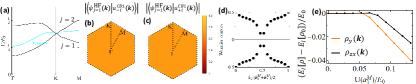
Figure S9: (a) The spectrum of $H^{\text{HF}}({\textbf{{k}}})$ for the mirror coherent states with $\rho^{\text{R}}_{zx}({\textbf{{k}}})$ (black lines) . (b)(c) The overlap between mirror coherent states $|\psi^{\text{H}F}_{j=1}({\textbf{{k}}})\rangle$ for the filled band in (a) and the non interacting states $|u^{\text{CB1}}_{\pm i}\rangle({\textbf{{k}}})$. (d) The Wannier center flow for both eigen-states of $H^{\text{HF}}({\textbf{{k}}})$. (e) The energy per particle $E_{\text{I}}[\rho^{\text{R}}]$ with non-interacting energy $E_{\text{I}}[\rho_{0}]$ subtracted for $\rho^{\text{R}}_{y}({\textbf{{k}}})$ and $\rho^{\text{R}}_{zx}({\textbf{{k}}})$. Here the calculation is for the two-band model with the parameters $\phi=0,\alpha=1,V_{0}/E_{0}=0$.

For $\rho^{\text{R}}_{zx}({\textbf{{k}}})$, the initial density matrices are taken as

$$\rho^{\text{R}}_{ini}=\frac{1}{2}(\sigma_{0}+\sigma_{z}\cos 2\tilde{\varphi}-\sigma_{x}\sin 2\tilde{\varphi})$$ (S78)

for a certain uniform value of $\tilde{\varphi}$, which corresponds to states $\cos\tilde{\varphi}|u^{\text{R},\text{CB1}}_{+}({\textbf{{k}}})\rangle-\sin\tilde{\varphi}|u^{\text{R},\text{CB1}}_{-}({\textbf{{k}}})\rangle$. The HF energy spectrum from this initial $\rho^{\text{R}}_{ini}$ in Fig. S9 shows nodes at $K,K^{\prime}$. These nodes can be understood from nonzero Euler number, denoted as $\mu$, a topological invariant defined for a two-band model with the $C_{2z}\mathcal{T}$ symmetry Bouhon et al. (2020); Yu et al. (2022); Ahn et al. (2019). The non-interacting eigen-state of CB1 has non-trivial $\mathbb{Z}_{2}$ number $\nu_{\text{CB1}}=1$, and the Euler number can be related to the $\mathbb{Z}_{2}$ number by $\nu_{CB1}=\mu\mod 2$Ahn et al. (2019). Thus, when $\nu_{\text{CB1}}=1$, $\mu$ has to be an odd number, which gives rise to $2\mu$ of gapless Dirac nodes in the spectrum. Because $C_{2z}\mathcal{T}$ is preserved for the initial density matrix $\rho^{\text{R}}_{ini}$, this symmetry remains throughout the whole self-consistent calculation process, so Euler class is still well-defined for the final self-consistent Hatree-Fock ground state. We evaluate the Wannier center flow for the final Hatree-Fock ground state, which is shown in Fig. S9(d). The nonzero Euler class with $\mu=1$ from the Wannier center flow guarantees the existence of $2$ Dirac nodes in the Hartree-Fock spectrum. Fig. S9(b)(c) shows that the Hartree-Fock solutions $|\psi^{\text{HF}}_{j=1}({\textbf{{k}}})\rangle$ shown in Fig. S9(a) are superposition of two $m_{z}$ states with the same probability

$$|\langle\psi^{\text{HF}}_{j=1}({\textbf{{k}}})|u^{\text{CB1}}_{-i}({\textbf{{k}}})\rangle|=1/\sqrt{2}\quad|\langle\psi^{\text{HF}}_{j=1}({\textbf{{k}}})|u^{\text{CB1}}_{+i}({\textbf{{k}}})\rangle|=1/\sqrt{2},$$ (S79)

which are denoted as mirror coherent states.

The true ground state of the system is obtained by comparing the energies $E_{\text{I}}[\rho^{\text{R}}]$ of two self-consistent density matrices in Fig. S9(e). Above the critical interaction value around $0.05E_{0}\approx 2$ meV, our calculation shows that the mirror polarized state with $\rho^{\text{R}}_{y}({\textbf{{k}}})$ has lower energies than the non-interacting ground state and the mirror coherent states with $\rho^{\text{R}}_{zx}({\textbf{{k}}})$. This is because non-interacting ground state and mirror coherent state have gapless excitations in their spectrum, while the mirror polarized states are fully gapped. Thus, we conclude that the true ground state is a mirror polarized Chern insulator.

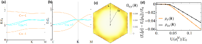
Figure S10: (a)(b) The spectra (orange) of $H^{\text{HF}}({\textbf{{k}}})$ with $\rho^{\text{R}}_{y}({\textbf{{k}}})$ for (a) and $\rho^{\text{R}}_{zx}({\textbf{{k}}})$ for (b). The cyan lines are non-interacting spectrum. (c) Berry curvature for the lower band of $H^{\text{HF}}({\textbf{{k}}})$ in (a). (c) The energy per particle $E_{\text{I}}[\rho^{\text{R}}]$ with non-interacting energy $E_{\text{I}}[\rho_{0}]$ subtracted for $\rho^{\text{R}}_{y}({\textbf{{k}}})$ and $\rho^{\text{R}}_{zx}({\textbf{{k}}})$. Here the calculation is for the two-band model with the parameters $\phi=0,\alpha=0,V_{0}/E_{0}=1.2$.

For the case with $\alpha=0,V_{0}/E_{0}=1.2,\phi=0$ without inversion, the mirror symmetry $\mathcal{M}_{z}$ is broken so we cannot characterize the non-interacting eigen-state with mirror eigen-values and mirror Chern number. However, the $C_{2z}\mathcal{T}$ symmetry remains, so we can still choose the real gauge for non-interacting states as $|u^{\text{R,CB1}}_{1}({\textbf{{k}}})\rangle,|u^{\text{R,CB1}}_{2}({\textbf{{k}}})\rangle$, which satisfies

$$C_{2z}\mathcal{T}|u^{\text{R,CB1}}_{n}({\textbf{{k}}})\rangle=|u^{\text{R,CB1}}_{n}({\textbf{{k}}})\rangle,$$ (S80)

where $n=1,2$ labels two spin-split bands for the Kramers’ pair of CB1. Consequently, two types of order parameters, $\rho^{\text{R}}_{y}({\textbf{{k}}})$ that breaks $C_{2z}\mathcal{T}$ and $\rho^{\text{R}}_{zx}({\textbf{{k}}})$ that breaks spin $U(1)$ symmetry, do not mix with each other. The self-consistent solutions with two types of order parameters are shown in Fig. S10. $\rho^{\text{R}}_{y}({\textbf{{k}}})$ breaks $\mathcal{T}$ symmetry and one band of CB1 with nonzero Chern number is gapped from the other band. $\rho^{\text{R}}_{zx}({\textbf{{k}}})$ has Dirac nodes in spectra at $K,K^{\prime}$ with energies $E_{\text{I}}[\rho^{\text{R}}_{zx}({\textbf{{k}}})]$ higher than the other case. The ground state is an interaction-driven Chern insulator, same as the inversion symmetric case.

II.4 Four-band model with CB1 and CB2

In the main text, we have discussed the important role of the band mixing between CB1 and CB2 induced by the Coulomb interaction, which can result in the interacting ground state varying from the QAH state to a trivial insulator state for the realistic Coulomb interaction strength for the inversion symmetric case ($V_{0}=0$), while the QAH state remains for the realistic Coulomb interaction when a large asymmetric potential $V_{0}$ is applied. The difference between the inversion symmetric and asymmetric cases is that both CB1 and CB2 carry non-trivial $\mathbb{Z}_{2}$ number, $\nu_{CB1}=\nu_{CB2}=1$, for inversion symmetric case, while a strong asymmetric potential $V_{0}$ gives a trivial insulator phase for CB2, $\nu_{CB1}=1$ and $\nu_{CB2}=0$, for inversion asymmetric case. This effect can only be taken into account when considering both CB1 and CB2, and thus it is important to go beyond the two-band model discussed above and consider a four-band model with both CB1 and CB2. In this section, we will provide more details of our numerical self-consistent calculations of the interacting ground state within the HF approximations for the four-band model. Below we always assume the $1/4$ filling of four bands, which corresponds to the $1/2$ filling of CB1.

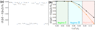
Figure S11: (a) The energy per particle for the self-consistent Hartree-Fock solutions labelled by initial density matrix $\rho_{ini}$ for $U(a_{1}^{\text{M}})=0.13E_{0}$. (b) The energy per particle for the self-consistent Hartree-Fock solutions under different interaction strength. Orange (Black) lines are $C_{2z}\mathcal{T}$ symmetry breaking (preserving) states. Here the calculation is for the four-band model with the parameters $\phi=0,\alpha=1,V_{0}/E_{0}=0$

.

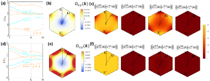
Figure S12: (a) The spectra (orange) of $H^{\text{HF}}({\textbf{{k}}})$ with $\rho^{\text{R}}_{ini}({\textbf{{k}}})=\tau_{0}\sigma_{y}$ and $U(a_{1}^{\text{M}})=0.13E_{0}$. The cyan lines are non-interacting spectrum. (b) Berry curvature for the lowest band $j=1$ of $H^{\text{HF}}({\textbf{{k}}})$ in (a). (c) The overlap between the ground states $|\tilde{\psi}^{\text{HF}}_{j=1}({\textbf{{k}}})\rangle$ in (a) and the non-interacting states $|u^{\text{R,CB1/CB2}}_{\pm i}({\textbf{{k}}})\rangle$. (d)(e)(f) are same as (a)(b)(c), respectively, for $U(a_{1}^{\text{M}})=0.08E_{0}$. Here the calculation is for the four-band model with the parameters $\phi=0,\alpha=1,V_{0}/E_{0}=0$.

For the case $\alpha=1,V_{0}/E_{0}=0,\phi=0$ with inversion symmetry, the non-interacting states now have $|u^{\text{CB1}}_{\pm i}({\textbf{{k}}})\rangle$ with $C=\pm 1$ and $|u^{\text{CB2}}_{\pm i}({\textbf{{k}}})\rangle$ with $C=\mp 1$, where $C$ denotes the Chern number of the mini-bands in the $m_{z}=-i$ subspace (mirror Chern number). For the convenience of the calculations, we choose the real gauge by applying the transformation given in Eq. (S65) to the basis wave-functions for both CB1 and CB2, denoted as $|u^{\text{ R,CB1}}_{\pm}\rangle,|u^{\text{ R,CB2}}_{\pm}\rangle$. The initial density matrices $\rho^{\text{R}}_{ini}$ are taken as one of $\tau_{i}\sigma_{j}$ with $i,j=0,x,y,z$ and $\tau$ acting on CB1,CB2 and $\sigma$ acts on two real basis in one Kramer pair of bands, which are all possible $4\times 4$ uniform density matrices. From $E_{I}[\rho^{\text{R}}({\textbf{{k}}})]$ for different $\rho^{\text{R}}_{ini}$ in Fig. S11, the self-consistent solutions can also be divided into two groups: one with complex density matrices breaking $C_{2z}\mathcal{T}$ (e.g. $\tau_{i}\sigma_{y}$ and $\tau_{y}\sigma_{i}$ with $i=0,x,z$) and the other with real density matrices preserving breaking $C_{2z}\mathcal{T}$ (e.g. $\tau_{i}\sigma_{j}$ with $i,j=0,x,z$ and $\tau_{y}\sigma_{y}$), as the $C_{2z}\mathcal{T}$ symmetry is preserved at the single-particle Hamiltonian level for $\phi=0$. We generally find that the self-consistent solutions with the initial complex density matrices have lower energies, as shown in Fig. S11(a). Although the initial density matrices $\rho^{\text{R}}_{ini}$ are different, we numerically find the self-consistent density matrices are all mirror polarized states related by $C_{2z}$ or $\mathcal{T}$. From Fig.4(a) in the main text or Fig. S11(b) reproduced here, the self-consistent solutions with complex density matrices becomes the ground states when the Coulomb interaction exceeds $0.04E_{0}$. The inter-band mixing between CB1 and CB2 is negligible for interaction strength in regime II with $0.04E_{0}<U(a^{M}_{1})<0.09E_{0}$ but a strong band mixing is found in regime III with larger Coulomb interaction $0.09E_{0}<U(a^{M}_{1})$. Fig. S12 shows the self-consistent solutions for the initial density matrix $\rho^{\text{R}}_{ini}=\tau_{0}\sigma_{y}$ as an example. Here Fig. S12(a)-(c) are for $U(a_{1}^{\text{M}})=0.13E_{0}$ (regime III) while (d)-(f) are for $U(a_{1}^{\text{M}})=0.08E_{0}$ (regime II). The filled band $|\tilde{\psi}^{\text{HF}}_{j=1}({\textbf{{k}}})\rangle$ in Fig. S12(a) for regime III has the Chern number $C=0$ and that in Fig. S12(d) for regime II has $C=+1$. Fig. S12(b) and (e) show the distribution of Berry curvature $\Omega_{xy}$ in the moiré BZ for regime III and regime II, respectively. Fig. S12(c) and (f) show the projection of $|\tilde{\psi}^{\text{HF}}_{j=1}({\textbf{{k}}})\rangle$ into non-interacting states $|u^{\text{CB1}}_{\pm i}({\textbf{{k}}})\rangle$ and $|u^{\text{CB2}}_{\pm i}({\textbf{{k}}})\rangle$ in regime III and regime II, respectively. One can see that the interacting ground state $|\tilde{\psi}^{\text{HF}}_{j=1}({\textbf{{k}}})\rangle$ has a strong component from $|u^{\text{CB2}}_{\pm i}({\textbf{{k}}})\rangle$, in addition to $|u^{\text{CB1}}_{\pm i}({\textbf{{k}}})\rangle$, due to the strong band mixing in regime III, while only the $|u^{\text{CB1}}_{\pm i}({\textbf{{k}}})\rangle$ part dominates the interacting ground state in regime II. Thus, from Fig. S12, we show that the Coulomb interaction can drive the interacting ground state into a trivial Mott insulator phase Sorella and Tosatti (1992); Neto et al. (2009) via band mixing between CB1 and CB2 when there is inversion symmetry.

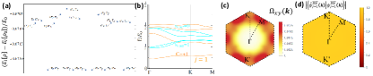
Figure S13: (a) The energies of the self-consistent Hartree Fock states with different initial density matrices $\rho^{\text{R}}_{ini}({\textbf{{k}}})$. (b) The spectra (orange) of $H^{\text{HF}}({\textbf{{k}}})$ with $\rho^{\text{R}}_{ini}({\textbf{{k}}})=\sigma_{y}\tau_{0}$ and $U(a_{1}^{\text{M}})=0.13E_{0}$. The cyan lines are non-interacting spectrum. (c) Berry curvature for the lowest band of $H^{\text{HF}}({\textbf{{k}}})$ in (b). (d) The overlap between the ground states $|\tilde{\psi}^{\text{HF}}_{j=1}({\textbf{{k}}})\rangle$ for four-band Hartree-Fock calculations and the ground states $|\psi^{\text{HF}}_{j=1}({\textbf{{k}}})\rangle$ for two-band Hartree-Fock calculations. Here the calculation is for the four-band model with the parameters $\phi=0,\alpha=0,V_{0}/E_{0}=1.2$.

For the case $\alpha=0,V_{0}/E_{0}=1.2,\phi=0$ without inversion symmetry, the self-consistent solutions are summarized in Fig. S13. As shown in the phase diagram of Fig. 4(b) in the main text, the system stays in the QAH state with $C=+1$ for the realistic Coulomb interaction strength $U(a_{1}^{\text{M}})=U_{0}\approx 0.13E_{0}$, which is quite different from the inversion symmetric case. Here we show more details of this calculation in Fig. S13 for $U(a_{1}^{\text{M}})=0.13E_{0}$. Fig. S13(a) shows that the self-consistent solutions with the initial complex density matrices that break the $C_{2z}\mathcal{T}$ still have lower energy. We consider $\sigma_{0}\tau_{y}$ as an example and show the energy dispersion of HF bands in Fig. S13(b). The distribution of the Berry curvature $\Omega_{xy}$ in the moiré BZ is shown in Fig. S13(c). We further project the interacting ground state of the four-band model, denoted as $|\tilde{\psi}^{\text{HF}}_{j=1}({\textbf{{k}}})\rangle$, into that of the two-band model, denoted as $|\psi^{\text{HF}}_{j=1}({\textbf{{k}}})\rangle$, and find their overlap is almost 1 in the whole moiré BZ, as shown in Fig. S13(d). Thus, the inter-band mixing is negligible in the inversion asymmetric case for $U(a_{1}^{\text{M}})=U_{0}\approx 0.13E_{0}$.

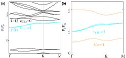
Figure S14: (a) Spectrum for the moiré system for smaller moiré unit cells. (b) The spectra (orange) of $H^{\text{HF}}$ with $\rho^{\text{R}}_{y}({\textbf{{k}}})$ for mirror polarized states. Here the calculation is for the two-band model with the parameters $\phi=1/3,\alpha=0.16,V_{0}/E_{0}^{\prime}=1.1$.

II.5 Coulomb interaction for smaller moiré unit cells

In this section, we discuss the moiré systems with a smaller moiré lattice constant, $|{\textbf{{a}}}_{1}^{\text{M}}|=14$nm, for a twist angle $\theta=1.0^{\circ}$. The Coulomb interaction scales inversely with the moiré unit cell length and its strength can be estimated as $U({\textbf{{a}}}_{1}^{\text{M}})=10$ meV.

The spectrum is shown in Fig. S14(a). The parameters for the spectrum are $\Delta_{1}=14$meV, $\phi=1/3$, and $m_{0}=30$meV. The energy scale is $E_{0}^{\prime}=v|{\textbf{{b}}}_{1}^{\text{M}}|=77$meV. The bandwidth of CB1 is $7.4$meV and the direct gap between CB1 and CB2 is $4$meV. The ratio between $U({\textbf{{a}}}_{1}^{\text{M}})$ and bandwidth is smaller for the smaller $|{\textbf{{a}}}_{1}^{\text{M}}|$. When the Coulomb interaction is considered for CB1 with the density matrix $\rho^{\text{R}}_{y}({\textbf{{k}}})$ as shown in Fig. S14(b), the mirror polarized states with $C=+1$ can be induced.

III Computational Methods for DFT calculations and moiré lattice

The DFT calculations were performed with the Vienna Ab initio Simulation Package (VASP)${}^{\cite[cite]{\@@bibref{Authors Phrase1YearPhrase2}{kresse1996efficient}{\@@citephrase{(}}{\@@citephrase{)}}}}$. The exchange-correlation functional was chosen as the Perdew-Burke-Ernzerhof type generalized-gradient approximation${}^{\cite[cite]{\@@bibref{Authors Phrase1YearPhrase2}{perdew1996generalized}{\@@citephrase{(}}{\@@citephrase{)}}}}$ and the projector-augmented-wave method was used for the core-electron potentials${}^{\cite[cite]{\@@bibref{Authors Phrase1YearPhrase2}{blochl1994projector,kresse1999ultrasoft}{\@@citephrase{(}}{\@@citephrase{)}}}}$. The energy cutoff was set as 340 eV for all calculations. The convergence criterion was set as 10^-5 eV for self-consistent electronic calculations and the $k$-point meshes were set as $13\times 13\times 1$ to sample the Brillouin zone. We used the DFT-D3 method${}^{\cite[cite]{\@@bibref{Authors Phrase1YearPhrase2}{grimme2010consistent}{\@@citephrase{(}}{\@@citephrase{)}}}}$ to correctly describe the van der Waals interactions.

As discussed in the main text and the next section IV, the moiré potential $\Delta({\textbf{{r}}})$ in the twisted Sb₂/Sb₂Te₃ hetero-structures could be obtained from the uniform potential $\tilde{\Delta}({\textbf{{d}}}_{{\textbf{{R}}}})$ for the hetero-structure with a uniform shift ${\textbf{{d}}}_{{\textbf{{R}}}}$ between the Sb₂ layer and Sb₂Te₃ layer. Therefore, we will describe below our first principles calculations of the band structures with different stacking configurations that correspond to different shifting vectors ${\textbf{{d}}}_{{\textbf{{R}}}}$. As shown in Fig. S15(a), the heterostructure model with the specific stacking contains $1\times 1$ Sb₂ monolayer and $1\times 1$ 2QL Sb₂Te₃ thin film. A vacuum layer with 20 Å was added along the z direction to avoid the interaction between adjacent slabs. Because the uniform potential $\tilde{\Delta}({\textbf{{d}}}_{{\textbf{{R}}}})$ is induced by coupling between Sb₂ monolayer and Sb₂Te₃ thin films, we fixed the value of the van der Waals gap inside 2QL Sb₂Te₃ thin film as the bulk value (2.708 Å), and then let Sb₂ monolayer and its neighboring atoms fully relax until the calculated forces are smaller than 0.01 eV/Å. In Fig. 5 of the main text, we plot the relaxed lattices and corresponding band structures for heterostructures with AA, AB, and BA stacking, whose interlayer distances between Sb₂ monolayer and 2QL Sb₂Te₃ thin film are 3.92 Å, 2.81 Å, and 2.91 Å respectively.

Besides the stacking configurations shown in the main text, other stacked heterostructures can be also found in the moiré pattern (see Fig. 5 in the main text). In order to calculate moiré potential $\Delta({\textbf{{r}}})$ accurately (see Section IV below), we consider extra nine stacked configurations, as shown in Fig. S15(b-d), which are located in the intermediate regions among AA, AB, and BA stackings, named AAmAA-X (Fig. S15(b)), AAmAB-X (Fig. S15(c)), and AAmBA-X (Fig. S15(d)) with X = I, II, III. We take the heterostructure models with AAmAA stackings as an example to show their lattices in details and the other intermediate stacked configurations could be obtained by using the same method. There are three types of AAmAA stacked structures in the moiré pattern, corresponding to the shifting vector ${\textbf{{d}}}_{R}$ as $\tilde{{\textbf{{a}}}}_{1}/2+0\tilde{{\textbf{{a}}}}_{2}$, $0\tilde{{\textbf{{a}}}}_{1}-\tilde{{\textbf{{a}}}}_{2}/2$, and $\tilde{{\textbf{{a}}}}_{1}/2+\tilde{{\textbf{{a}}}}_{2}/2$ for AAmAA-I, AAmAA-II, and AAmAA-III respectively. These three configurations are related by C_3z rotation, and thus we only need to calculate the electronic structure for one of them. On the other hand, because these intermediate stacked structures are not in the local minimum of the potential energy surface, we only relax the $z$ direction coordinate while fix the $x$ and $y$ coordinates of the Sb₂ monolayer (see Fig. S15(a)). The corrugation effect, which is crucial for predicting the correct band structure in twisted bilayer grapheneLucignano et al. (2019); Uchida et al. (2014); Koshino et al. (2018), is taken into account after this lattice relaxation process. Using the same method, we obtained the relaxed intermediate stacked heterostructures for AAmAB-X and AAmBA-X (X = I, II, III). The interlayer distances between Sb₂ monolayer and 2QL Sb₂Te₃ thin film are 2.94 Å, 3.38 Å, and 3.42 Å for AAmAA, AAmAB, and AAmBA stacked heterostructures respectively and the related band structures are shown in Fig. S15(e) correspondingly.

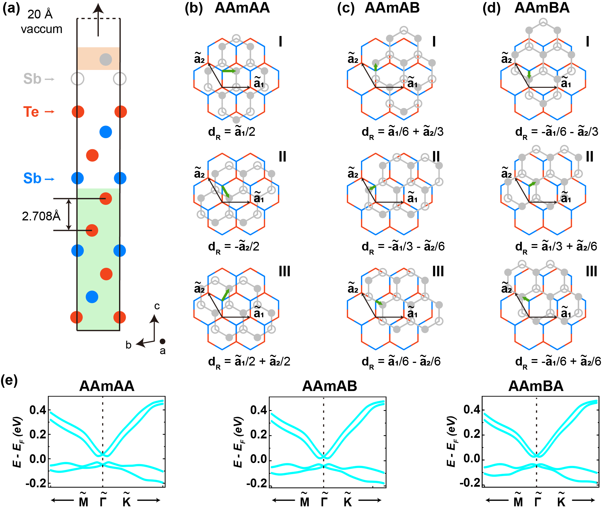
Figure S15: (a) The side view of the Sb₂/Sb₂Te₃ heterostructure with AA stacking. The solid black lines mark the unitcell used in DFT calculations. Sb atoms in Sb₂ monolayer are marked as gray, Sb atoms and Te atoms in Sb₂Te₃ films are marked as red and blue. The atoms in the region with the green background are frozen when we relax the lattice structures, the $x$ and $y$ coordinates of Sb atoms in the region with the yellow background are fixed. The value of the van der Waals gap inside 2QL Sb₂Te₃ films is 2.078Å. (b-d) The top view for heterostructures with the stacking of AAmAA-X, AAmAB-X, and AAmBA-X (X = I, II, III). Corresponding ${\textbf{{d}}}_{R}$ is shown by the green arrows. The black arrows show the lattice vector of Sb₂ monolayer. (e) Calculated band structures of the heterostructure with the stacking of AAmAA, AAmAB, and AAmBA, respectively. The Fermi levels are set as zero.

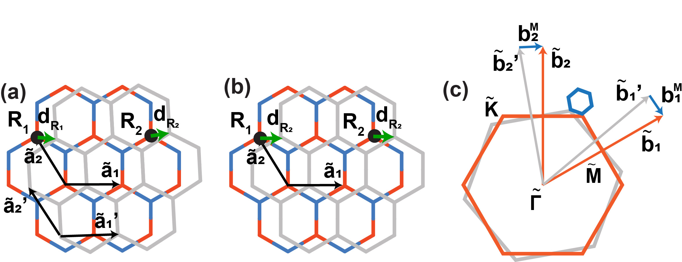
Figure S16: (a) The lattice structures for the twisted Sb₂ (gray) on top of Sb₂Te₃ (blue and orange) at a location same as Fig.4(c) of the main text. $\tilde{{\textbf{{a}}}}_{1,2}$ are primitive lattice vectors for the Sb₂Te₃ layer and $\tilde{{\textbf{{a}}}}_{1,2}^{\prime}$ are primitive lattice vectors for Sb₂ layer. ${\textbf{{d}}}_{{\textbf{{R}}}_{1,2}}$ are the local lattice shifts at sites ${\textbf{{R}}}_{1,2}$. (b) Commensurate Sb₂ (gray) on top of Sb₂Te₃ with a constant shift ${\textbf{{d}}}_{{\textbf{{R}}}_{2}}$ as an approximation for the local lattice structures in (a). (c) BZs for Sb₂Te₃ (orange), Sb₂ (gray), and moiré superlattice (blue). $\tilde{{\textbf{{b}}}}_{1,2}$, $\tilde{{\textbf{{b}}}}_{1,2}^{\prime}$, $\tilde{{\textbf{{b}}}}^{\text{M}}_{1,2}$ are reciprocal lattice vectors for for Sb₂Te₃, Sb₂, moiré superlattice, respectively.

IV Moiré potentials from the fitting to the DFT band structure

In this section, we discuss the method to obtain Moire potential $\Delta({\textbf{{r}}})$ in Eq. 1 of the main text from the above DFT calculation in Sec. III Jung et al. (2014).

We first consider the effective Hamiltonian $H^{\text{DFT}}$ in Eq. (3) of the main text. Compared to the original Hamiltonian $H_{0}$ in Eq. 1, the spatially dependent moiré potential term $\Delta({\textbf{{r}}})$ is changed to a uniform potential term $\tilde{\Delta}({\textbf{{d}}}_{R})$ for a fixed ${\textbf{{d}}}_{R}$ that describes the relative shift between Sb₂ and Sb₂Te₃ layers. $H^{\text{DFT}}$ describes the effective model for the hetero-structure with a uniform shift between two atomic layers, and different values of the shifting vector ${\textbf{{d}}}_{R}$ describe different stacking configurations. Thus, we can use the energy dispersion of $H^{\text{DFT}}$ to fit to that from the DFT calculations.

The effective Hamiltonian $\hat{H}^{\text{DFT}}({\textbf{{d}}}_{R})$ is then given by

$$\langle{\textbf{{k}}}_{1},\beta_{1}|\hat{H}^{\text{DFT}}({\textbf{{d}}}_{R})|{\textbf{{k}}}_{2},\beta_{2}\rangle=\delta({\textbf{{k}}}_{1}-{\textbf{{k}}}_{2})(\begin{pmatrix}h_{D}^{t}({\textbf{{k}}}_{1})&ms_{0}\\ ms_{0}&h_{D}^{b}({\textbf{{k}}}_{1})\end{pmatrix}+\begin{pmatrix}\tilde{\Delta}({\textbf{{d}}}_{R})s_{0}&0\\ 0&\alpha\tilde{\Delta}({\textbf{{d}}}_{R})s_{0}\end{pmatrix})=\delta({\textbf{{k}}}_{1}-{\textbf{{k}}}_{2})H^{\text{DFT}}({\textbf{{k}}}_{1},{\textbf{{d}}}_{\textbf{{R}}}),$$ (S81)

where $H^{\text{DFT}}({\textbf{{k}}},{\textbf{{d}}}_{\textbf{{R}}})$ is just Eq.(4) in the main text, $h_{D}^{t/b}({\textbf{{k}}})$ are the top/bottom Dirac surface states same as Eq. (1) of the main text, $s_{0}$ are the identical matrix in spin space, $m$ is the tunnelling between two surfaces, and $\alpha$ captures the difference in the potentials on two surfaces created by the Sb₂ layer. $|{\textbf{{k}}},\beta\rangle$ is the atomic Bloch states for the Sb₂Te₃ and Sb₂ lattice with a constant shift. $\beta_{1,2}=1,...,4$ represents both the spin and layer degrees of freedom. The spectra of this model are given by

$$E^{\text{DFT}}_{\eta,\xi}({\textbf{{k}}},{\textbf{{d}}})=\frac{1+\alpha}{2}\tilde{\Delta}({\textbf{{d}}})+\eta\sqrt{m^{2}+\left(\frac{1-\alpha}{2}\tilde{\Delta}({\textbf{{d}}})+\xi v^{2}k^{2})\right)^{2}}.$$ (S82)

with $\eta=\pm,\xi=\pm$. By fitting $E^{\text{DFT}}_{\eta,\xi}({\textbf{{k}}},{\textbf{{d}}})$ to the spectrum calculated from DFT in Fig.4(b) of the main text and Fig. S15(f), the parameters $\alpha$, $\tilde{\Delta}({\textbf{{d}}})$, $v$ and $m$ in the model Hamiltonian can be obtained. From the three-fold rotation symmetry $C_{3}$ of the underlying lattice, one can obtain

$$\langle{\textbf{{k}}},\beta_{1}|\hat{H}^{\text{DFT}}({\textbf{{d}}})|{\textbf{{k}}},\beta_{2}\rangle=\langle C_{3}{\textbf{{k}}},\beta_{1}|\hat{H}^{\text{DFT}}(C_{3}{\textbf{{d}}})|C_{3}{\textbf{{k}}},\beta_{2}\rangle$$ (S83)

and

$$E^{\text{DFT}}_{\eta,\xi}({\textbf{{k}}},{\textbf{{d}}})=E^{\text{DFT}}_{\eta,\xi}(C_{3}{\textbf{{k}}},C_{3}{\textbf{{d}}})=E^{\text{DFT}}_{\eta,\xi}({\textbf{{k}}},C_{3}{\textbf{{d}}}),$$ (S84)

where the last line following from $E^{\text{DFT}}_{\eta,\xi}$ depends on $|{\textbf{{k}}}|$ in Eq. (S82). So, only one of three stacking related by $C_{3}$ shown in Fig. S15(b)-(d) needs to be fitted.

Next we will establish the relation between the moiré Hamiltonian $H_{0}$ in Eq.1 of the main text and the Hamiltonian $H^{\text{DFT}}$ constructed from the fitting to the DFT energy spectrum. We start from the momentum-space moiré Hamiltonian $\langle{\textbf{{k}}}_{1},\beta_{1}|\hat{H}_{0}|{\textbf{{k}}}_{2},\beta_{2}\rangle$ in Eq.1 of the main text, where $\beta_{1,2}=1,\cdots,4$ label both layer and spin indices and $|{\textbf{{k}}},\beta\rangle$ are atomic Bloch states for each layer underlying the moiré superlattice. As the moiré Hamiltonian $H_{0}$ does not preserve atomic lattice translation, the crystal momentum k is not a good quantum number and $H_{0}$ can mix different k states. The atomic Bloch wave function $|{\textbf{{k}}},\beta\rangle$ is related to atomic Wannier function $|{\textbf{{R}}},\beta\rangle$ by

$$|{\textbf{{k}}},\beta\rangle=\sum_{{\textbf{{R}}}}e^{i{\textbf{{k}}}\cdot{\textbf{{R}}}}|{\textbf{{R}}},\beta\rangle,$$ (S85)

so the moiré Hamiltonian is transformed into the form on the atomic Wannier function basis as

$$\langle{\textbf{{k}}}_{1},\beta_{1}|\hat{H}_{0}|{\textbf{{k}}}_{2},\beta_{2}\rangle=\sum_{{\textbf{{R}}}_{1}{\textbf{{R}}}_{2}}e^{-i{\textbf{{k}}}_{1}\cdot{\textbf{{R}}}_{1}}\langle{\textbf{{R}}}_{1},\beta_{1}|\hat{H}_{0}|{\textbf{{R}}}_{2},\beta_{2}\rangle e^{i{\textbf{{k}}}_{2}\cdot{\textbf{{R}}}_{2}}.$$ (S86)

Here $\langle{\textbf{{R}}}_{1},\beta_{1}|\hat{H}_{0}|{\textbf{{R}}}_{2},\beta_{2}\rangle$ describes the Hamiltonian matrix element between atomic Wannier functions located at ${\textbf{{R}}}_{1}$ and ${\textbf{{R}}}_{2}$ in the superlattice shown in Fig. S16(a). As the overlap between atomic Wannier functions decays quickly as the distance increases, we only consider the local hopping within the length scale $|{\textbf{{R}}}_{2}-{\textbf{{R}}}_{1}|\sim\mathcal{O}(|\tilde{{\textbf{{a}}}}_{1}|)$, where $\tilde{{\textbf{{a}}}}_{1}$ is the atomic primitive lattice vector for the Sb₂Te₃ layer. In this atomic length scale, the Hamiltonian matrix element between two Wannier orbitals near R on the superlattice structure with twist angle $\theta$ in Fig. S16(a) can be approximated locally by the Hamiltonian matrix element for two atomic layers with a constant shift ${\textbf{{d}}}_{\textbf{{R}}}$ in Fig. S16(b)Jung et al. (2014), where

$${\textbf{{d}}}_{\textbf{{R}}}=\mathcal{R}(\theta){\textbf{{R}}}-{\textbf{{R}}}$$ (S87)

and $\mathcal{R}(\theta)$ as the rotation operator for the Sb₂ layer with the rotating angle $\theta$. This approximation is valid for a small twist angle $\theta$ because the local shift vector ${\textbf{{d}}}_{\textbf{{R}}}$ is almost uniform at the atomic length scale,

$${\textbf{{d}}}_{{\textbf{{R}}}_{2}}\approx{\textbf{{d}}}_{{\textbf{{R}}}_{1}}$$ (S88)

for $|{\textbf{{R}}}_{2}-{\textbf{{R}}}_{1}|\sim\mathcal{O}(|\tilde{{\textbf{{a}}}}_{1}|)$. The Hamiltonian matrix element between two atomic Wannier orbitals for the commensurate lattice is captured by $\langle{\textbf{{R}}}_{1},\beta_{1}|\hat{H}^{\text{DFT}}({\textbf{{d}}}_{{\textbf{{R}}}_{2}})|{\textbf{{R}}}_{2},\beta_{2}\rangle$, so we make the approximation

$$\langle{\textbf{{R}}}_{1},\beta_{1}|\hat{H}_{0}|{\textbf{{R}}}_{2},\beta_{2}\rangle\approx\langle{\textbf{{R}}}_{1},\beta_{1}|\hat{H}^{\text{DFT}}({\textbf{{d}}}_{{\textbf{{R}}}_{2}})|{\textbf{{R}}}_{2},\beta_{2}\rangle$$ (S89)

and

$$\langle{\textbf{{k}}}_{1},\beta_{1}|\hat{H}_{0}|{\textbf{{k}}}_{2},\beta_{2}\rangle=\sum_{{\textbf{{R}}}_{1}{\textbf{{R}}}_{2}}e^{-i{\textbf{{k}}}_{1}\cdot{\textbf{{R}}}_{1}}\langle{\textbf{{R}}}_{1},\beta_{1}|\hat{H}^{\text{DFT}}({\textbf{{d}}}_{{\textbf{{R}}}_{2}})|{\textbf{{R}}}_{2},\beta_{2}\rangle e^{i{\textbf{{k}}}_{2}\cdot{\textbf{{R}}}_{2}}.$$ (S90)

To extract ${\textbf{{R}}}_{2}$ in $\hat{H}^{\text{DFT}}({\textbf{{d}}}_{{\textbf{{R}}}_{2}})$ for the summation, we transform $\hat{H}^{\text{DFT}}({\textbf{{d}}}_{\textbf{{R}}})$ to the momentum-space by

$$\hat{H}^{\text{DFT}}({\textbf{{d}}}_{\textbf{{R}}})=\sum_{\tilde{{\textbf{{G}}}}}e^{-i\tilde{{\textbf{{G}}}}\cdot{\textbf{{d}}}_{\textbf{{R}}}}\hat{H}^{\text{DFT}}(\tilde{{\textbf{{G}}}})$$ (S91)

as $\hat{H}^{\text{DFT}}({\textbf{{d}}}_{\textbf{{R}}}+x\tilde{{\textbf{{a}}}}_{1}+y\tilde{{\textbf{{a}}}}_{2})=\hat{H}^{\text{DFT}}({\textbf{{d}}}_{\textbf{{R}}})$ is periodic for atomic lattice vectors ($x,y$ are integers here), as shown in Fig. S16(b). We also denote the atomic reciprocal lattice vector $\tilde{{\textbf{{G}}}}=\tilde{{\textbf{{G}}}}_{wz}=w\tilde{{\textbf{{b}}}}_{1}+z\tilde{{\textbf{{b}}}}_{2}$ with integers $w,z$, so the summation over $\tilde{{\textbf{{G}}}}$ is equivalent to the summation over $w,z$. $\tilde{{\textbf{{b}}}}_{1,2}$ are atomic reciprocal lattice vectors satisfying $\tilde{{\textbf{{b}}}}_{i}\cdot\tilde{{\textbf{{a}}}}_{j}=\delta_{ij}$ for $i,j=1,2$ and shown in Fig. S16(c). Since

$$\tilde{{\textbf{{G}}}}_{wz}\cdot{\textbf{{d}}}_{\textbf{{R}}}=\tilde{{\textbf{{G}}}}_{wz}\cdot(\mathcal{R}(\theta){\textbf{{R}}}-{\textbf{{R}}})=(\tilde{{\textbf{{G}}}}_{wz}-\mathcal{R}(\theta)\tilde{{\textbf{{G}}}}_{wz})\cdot(\mathcal{R}(\theta){\textbf{{R}}})={\textbf{{G}}}_{wz}\cdot({\textbf{{R}}}+{\textbf{{d}}}_{\textbf{{R}}})\approx{\textbf{{G}}}_{wz}\cdot{\textbf{{R}}}$$ (S92)

with the moiré reciprocal lattice vectors ${\textbf{{G}}}_{wz}$ given by

$$\begin{split}{\textbf{{G}}}_{wz}&=\tilde{{\textbf{{G}}}}_{wz}-\mathcal{R}(\theta)\tilde{{\textbf{{G}}}}_{wz}\\ &=(w\tilde{{\textbf{{b}}}}_{1}+z\tilde{{\textbf{{b}}}}_{2})-\mathcal{R}(\theta)(w\tilde{{\textbf{{b}}}}_{1}+z\tilde{{\textbf{{b}}}}_{2})\\ &=w(\tilde{{\textbf{{b}}}}_{1}-\mathcal{R}(\theta)\tilde{{\textbf{{b}}}}_{1})+z(\tilde{{\textbf{{b}}}}_{2}-\mathcal{R}(\theta)\tilde{{\textbf{{b}}}}_{2})\\ &=w(\tilde{{\textbf{{b}}}}_{1}-\tilde{{\textbf{{b}}}}_{1}^{\prime})+z(\tilde{{\textbf{{b}}}}_{2}-\tilde{{\textbf{{b}}}}_{2}^{\prime})\\ &=w{{\textbf{{b}}}_{1}^{\text{M}}}+z{{\textbf{{b}}}_{2}^{\text{M}}},\end{split}$$ (S93)

we have

$$e^{-i\tilde{{\textbf{{G}}}}\cdot{\textbf{{d}}}_{\textbf{{R}}}}\approx e^{-i{\textbf{{G}}}\cdot{\textbf{{R}}}},\quad\hat{H}^{\text{DFT}}({\textbf{{d}}}_{\textbf{{R}}})\approx\sum_{w,z}e^{-i{\textbf{{G}}}_{wz}\cdot{\textbf{{R}}}}\hat{H}^{\text{DFT}}(\tilde{{\textbf{{G}}}}_{wz}).$$ (S94)

Here $\tilde{{\textbf{{a}}}}_{1,2}^{\prime}=\mathcal{R}(\theta)\tilde{{\textbf{{a}}}}_{1,2}\ (\tilde{{\textbf{{b}}}}_{1,2}^{\prime}=\mathcal{R}(\theta)\tilde{{\textbf{{b}}}}_{1,2})$ are primitive (reciprocal) lattice vectors for the twisted Sb₂ layer as shown in Fig. S16(c) and ${\textbf{{b}}}_{1,2}^{\text{M}}=\tilde{{\textbf{{b}}}}_{1,2}-\tilde{{\textbf{{b}}}}_{1,2}^{\prime}$ are the moiré reciprocal lattice vectors. The approximation in Eq. (S92) is valid as $|{\textbf{{d}}}_{\textbf{{R}}}|\sim\mathcal{O}(|\tilde{{\textbf{{a}}}}_{1}|)\ll|{\textbf{{a}}}_{1}^{\text{M}}|$ and ${\textbf{{G}}}\cdot{\textbf{{d}}}_{\textbf{{R}}}\ll{\textbf{{G}}}\cdot{\textbf{{a}}}_{1}^{\text{M}}\sim\mathcal{O}(1)$.

Substituting Eq. (S89) and (S94) into Eq. (S86) leads to

$$\begin{split}\langle{\textbf{{k}}}_{1},\beta_{1}|\hat{H}_{0}|{\textbf{{k}}}_{2},\beta_{2}\rangle&\approx\sum_{{\textbf{{R}}}_{1}{\textbf{{R}}}_{2},w,z}e^{-i{\textbf{{k}}}_{1}\cdot{\textbf{{R}}}_{1}}e^{-i{\textbf{{G}}}_{wz}\cdot{\textbf{{R}}}_{2}}\langle{\textbf{{R}}}_{1},\beta_{1}|\hat{H}^{\text{DFT}}(\tilde{{\textbf{{G}}}}_{wz})|{\textbf{{R}}}_{2},\beta_{2}\rangle e^{i{\textbf{{k}}}_{2}\cdot{\textbf{{R}}}_{2}}\\ &=\sum_{w,z}\langle{\textbf{{k}}}_{1},\beta_{1}|\hat{H}^{\text{DFT}}(\tilde{{\textbf{{G}}}}_{wz})|{\textbf{{k}}}_{2}-{\textbf{{G}}}_{wz},\beta_{2}\rangle\\ &=\sum_{w,z}\delta({\textbf{{k}}}_{2}-{\textbf{{k}}}_{1}-{\textbf{{G}}}_{wz})\langle{\textbf{{k}}}_{1},\beta_{1}|\hat{H}^{\text{DFT}}(\tilde{{\textbf{{G}}}}_{wz})|{\textbf{{k}}}_{1},\beta_{2}\rangle.\end{split}$$ (S95)

The last line comes from the conservation of crystal momenta of $H^{\text{DFT}}({\textbf{{d}}})$,

$$\langle{\textbf{{k}}}_{1},\beta_{1}|\hat{H}^{\text{DFT}}(\tilde{{\textbf{{G}}}})|{\textbf{{k}}}_{2},\beta_{2}\rangle=\int\mathrm{d}^{2}{\textbf{{d}}}e^{i\tilde{{\textbf{{G}}}}\cdot{\textbf{{d}}}}\langle{\textbf{{k}}}_{1},\beta_{1}|\hat{H}^{\text{DFT}}({\textbf{{d}}})|{\textbf{{k}}}_{2},\beta_{2}\rangle=\delta({\textbf{{k}}}_{1}-{\textbf{{k}}}_{2})\langle{\textbf{{k}}}_{1},\beta_{1}|\hat{H}^{\text{DFT}}(\tilde{{\textbf{{G}}}})|{\textbf{{k}}}_{1},\beta_{2}\rangle.$$ (S96)

Eq. (S95) connects $H^{\text{DFT}}$ and $H_{0}$ in atomic Bloch states in general, which is applied to the moiré potential in our model next.

We next show the relation between the potential $\tilde{\Delta}({\textbf{{d}}}_{\textbf{{R}}})$ from DFT and the moiré potential $\Delta({\textbf{{r}}})$ in our model by Eq. (S95). The Fourier transform of $\langle{\textbf{{k}}},\alpha|\hat{H}^{\text{DFT}}({\textbf{{d}}}_{\textbf{{R}}})|{\textbf{{k}}},\alpha\rangle$ in Eq. (S81) by Eq. (S96) is

$$\langle{\textbf{{k}}},\beta_{1}|\hat{H}^{\text{DFT}}(\tilde{{\textbf{{G}}}})|{\textbf{{k}}},\beta_{2}\rangle=\begin{pmatrix}h_{D}^{t}({\textbf{{k}}})&ms_{0}\\ ms_{0}&h_{D}^{b}({\textbf{{k}}})\end{pmatrix}\delta_{\tilde{{\textbf{{G}}}}=0}+\begin{pmatrix}\tilde{\Delta}(\tilde{{\textbf{{G}}}})s_{0}&0\\ 0&\alpha\tilde{\Delta}(\tilde{{\textbf{{G}}}})s_{0}\end{pmatrix}.$$ (S97)

In atomic Bloch basis, the moiré Hamiltonian from Eq.1 of the main text without external electrical field is

$$\langle{\textbf{{k}}}_{1},\beta_{1}|\hat{H}_{0}|{\textbf{{k}}}_{2},\beta_{2}\rangle=\begin{pmatrix}h_{D}^{t}({\textbf{{k}}}_{1})&ms_{0}\\ ms_{0}&h_{D}^{b}({\textbf{{k}}}_{1})\end{pmatrix}\delta({\textbf{{k}}}_{2}-{\textbf{{k}}}_{1})+\begin{pmatrix}\Delta({\textbf{{G}}})s_{0}&0\\ 0&\alpha\Delta({\textbf{{G}}})s_{0}\end{pmatrix}\delta({\textbf{{k}}}_{2}-{\textbf{{k}}}_{1}-{\textbf{{G}}}).$$ (S98)

By comparison of two Hamiltonian following Eq. (S95), one obtains

$$\Delta({\textbf{{G}}}_{wz})=\tilde{\Delta}(\tilde{{\textbf{{G}}}}_{wz})$$ (S99)

for $w,z$ as integers, ${\textbf{{G}}}_{wz}=w{\textbf{{b}}}_{1}^{\text{M}}+z{\textbf{{b}}}_{2}^{\text{M}}$, and $\tilde{{\textbf{{G}}}}_{wz}=w\tilde{{\textbf{{b}}}}_{1}+z\tilde{{\textbf{{b}}}}_{2}$. In real space, this leads to

$$\Delta({\textbf{{R}}})=\sum_{w,z}e^{-i{\textbf{{G}}}_{w,z}\cdot{\textbf{{R}}}}\Delta({\textbf{{G}}}_{wz})\approx\sum_{w,z}e^{-i\tilde{{\textbf{{G}}}}_{w,z}\cdot(\mathcal{R}(\theta){\textbf{{R}}}-{\textbf{{R}}})}\tilde{\Delta}(\tilde{{\textbf{{G}}}}_{wz})=\tilde{\Delta}(\mathcal{R}(\theta){\textbf{{R}}}-{\textbf{{R}}})=\tilde{\Delta}({\textbf{{d}}}_{\textbf{{R}}})$$ (S100)

following Eq. (S92) and Eq. (S99), reproducing Eq. (4) in the main text. It then can be interpolated to the whole real space by replacing the atomic lattice vectors R by the continuous variable r,

$$\Delta({\textbf{{r}}})\approx\tilde{\Delta}(\mathcal{R}(\theta){\textbf{{r}}}-{\textbf{{r}}}),$$ (S101)

because the atomic length scale is much smaller than the moiré length scale for small twist angles so that it is a good approximation to take the continuous limit for the atomic length scale.

References

Bistritzer and MacDonald (2011)
R. Bistritzer and
A. H. MacDonald,
Proceedings of the National Academy of Sciences
108, 12233
(2011).
Cao et al. (2018a)
Y. Cao,
V. Fatemi,
A. Demir,
S. Fang,
S. L. Tomarken,
J. Y. Luo,
J. D. Sanchez-Yamagishi,
K. Watanabe,
T. Taniguchi,
E. Kaxiras,
et al., Nature
556, 80
(2018a).
Cao et al. (2018b)
Y. Cao,
V. Fatemi,
S. Fang,
K. Watanabe,
T. Taniguchi,
E. Kaxiras, and
P. Jarillo-Herrero,
Nature 556, 43
(2018b).
Sharpe et al. (2019)
A. L. Sharpe,
E. J. Fox,
A. W. Barnard,
J. Finney,
K. Watanabe,
T. Taniguchi,
M. Kastner, and
D. Goldhaber-Gordon,
Science 365,
605 (2019).
Yankowitz et al. (2019)
M. Yankowitz,
S. Chen,
H. Polshyn,
Y. Zhang,
K. Watanabe,
T. Taniguchi,
D. Graf,
A. F. Young, and
C. R. Dean,
Science 363,
1059 (2019).
Serlin et al. (2020)
M. Serlin,
C. Tschirhart,
H. Polshyn,
Y. Zhang,
J. Zhu,
K. Watanabe,
T. Taniguchi,
L. Balents, and
A. Young,
Science 367,
900 (2020).
Lu et al. (2019)
X. Lu,
P. Stepanov,
W. Yang,
M. Xie,
M. A. Aamir,
I. Das,
C. Urgell,
K. Watanabe,
T. Taniguchi,
G. Zhang,
et al., Nature
574, 653 (2019).
Kennes et al. (2021)
D. M. Kennes,
M. Claassen,
L. Xian,
A. Georges,
A. J. Millis,
J. Hone,
C. R. Dean,
D. Basov,
A. N. Pasupathy,
and A. Rubio,
Nature Physics 17,
155 (2021).
Zhang et al. (2017)
C. Zhang,
C.-P. Chuu,
X. Ren,
M.-Y. Li,
L.-J. Li,
C. Jin,
M.-Y. Chou, and
C.-K. Shih,
Science advances 3,
e1601459 (2017).
Mak and Shan (2022)
K. F. Mak and
J. Shan,
Nature Nanotechnology 17,
686 (2022).
Wu et al. (2018)
F. Wu,
T. Lovorn,
E. Tutuc, and
A. H. MacDonald,
Physical review letters 121,
026402 (2018).
Regan et al. (2020)
E. C. Regan,
D. Wang,
C. Jin,
M. I. Bakti Utama,
B. Gao,
X. Wei,
S. Zhao,
W. Zhao,
Z. Zhang,
K. Yumigeta,
et al., Nature
579, 359 (2020).
Tang et al. (2020)
Y. Tang,
L. Li,
T. Li,
Y. Xu,
S. Liu,
K. Barmak,
K. Watanabe,
T. Taniguchi,
A. H. MacDonald,
J. Shan, et al.,
Nature 579,
353 (2020).
Alexeev et al. (2019)
E. M. Alexeev,
D. A. Ruiz-Tijerina,
M. Danovich,
M. J. Hamer,
D. J. Terry,
P. K. Nayak,
S. Ahn,
S. Pak,
J. Lee,
J. I. Sohn,
et al., Nature
567, 81 (2019).
Jin et al. (2019)
C. Jin,
E. C. Regan,
A. Yan,
M. Iqbal Bakti Utama,
D. Wang,
S. Zhao,
Y. Qin,
S. Yang,
Z. Zheng,
S. Shi, et al.,
Nature 567, 76
(2019).
Seyler et al. (2019)
K. L. Seyler,
P. Rivera,
H. Yu,
N. P. Wilson,
E. L. Ray,
D. G. Mandrus,
J. Yan,
W. Yao, and
X. Xu,
Nature 567, 66
(2019).
Tran et al. (2019)
K. Tran,
G. Moody,
F. Wu,
X. Lu,
J. Choi,
K. Kim,
A. Rai,
D. A. Sanchez,
J. Quan,
A. Singh,
et al., Nature
567, 71 (2019).
Devakul et al. (2021)
T. Devakul,
V. Crépel,
Y. Zhang, and
L. Fu,
Nature communications 12,
1 (2021).
Chang et al. (2015a)
C.-Z. Chang,
P. Tang,
X. Feng,
K. Li,
X.-C. Ma,
W. Duan,
K. He, and
Q.-K. Xue,
Physical review letters 115,
136801 (2015a).
Salvato et al. (2022)
M. Salvato,
M. D. Crescenzi,
M. Scagliotti,
P. Castrucci,
S. Boninelli,
G. M. Caruso,
Y. Liu,
A. Mikkelsen,
R. Timm,
S. Nahas,
et al., ACS nano
16, 13860 (2022).
Schouteden et al. (2016)
K. Schouteden,
Z. Li,
T. Chen,
F. Song,
B. Partoens,
C. Van Haesendonck,
and K. Park,
Scientific reports 6,
1 (2016).
Yin et al. (2022)
Y. Yin,
G. Wang,
C. Liu,
H. Huang,
J. Chen,
J. Liu,
D. Guan,
S. Wang,
Y. Li,
C. Liu, et al.,
Nano Research 15,
1115 (2022).
Song et al. (2010)
C.-L. Song,
Y.-L. Wang,
Y.-P. Jiang,
Y. Zhang,
C.-Z. Chang,
L. Wang,
K. He,
X. Chen,
J.-F. Jia,
Y. Wang, et al.,
Applied Physics Letters 97,
143118 (2010).
Wang et al. (2012)
Y. Wang,
Y. Jiang,
M. Chen,
Z. Li,
C. Song,
L. Wang,
K. He,
X. Chen,
X. Ma, and
Q.-K. Xue,
Journal of Physics: Condensed Matter
24, 475604
(2012).
Liu et al. (2014)
Y. Liu,
Y. Li,
S. Rajput,
D. Gilks,
L. Lari,
P. Galindo,
M. Weinert,
V. Lazarov, and
L. Li,
Nature Physics 10,
294 (2014).
Xu et al. (2015)
S. Xu,
Y. Han,
X. Chen,
Z. Wu,
L. Wang,
T. Han,
W. Ye,
H. Lu,
G. Long,
Y. Wu, et al.,
Nano letters 15,
2645 (2015).
Vargas et al. (2017)
A. Vargas,
F. Liu,
C. Lane,
D. Rubin,
I. Bilgin,
Z. Hennighausen,
M. DeCapua,
A. Bansil, and
S. Kar,
Science advances 3,
e1601741 (2017).
Liu et al. (0)
B. Liu,
T. Wagner,
S. Enzner,
P. Eck,
M. Kamp,
G. Sangiovanni,
and R. Claessen,
Nano Letters 0,
null (0), pMID: 37027539,
eprint https://doi.org/10.1021/acs.nanolett.2c04974.
Cano et al. (2021)
J. Cano,
S. Fang,
J. Pixley, and
J. H. Wilson,
Physical Review B 103,
155157 (2021).
Dunbrack and Cano (2022)
A. Dunbrack and
J. Cano,
Physical Review B 106,
075142 (2022).
Wang et al. (2021)
T. Wang,
N. F. Yuan, and
L. Fu,
Physical Review X 11,
021024 (2021).
Lian et al. (2020)
B. Lian,
Z. Liu,
Y. Zhang, and
J. Wang,
Physical review letters 124,
126402 (2020).
Kane and Mele (2005)
C. L. Kane and
E. J. Mele,
Physical review letters 95,
226801 (2005).
Yu et al. (2010)
R. Yu,
W. Zhang,
H.-J. Zhang,
S.-C. Zhang,
X. Dai, and
Z. Fang,
science 329,
61 (2010).
Liu et al. (2010a)
C.-X. Liu,
X.-L. Qi,
H. Zhang,
X. Dai,
Z. Fang, and
S.-C. Zhang,
Physical Review B 82,
045122 (2010a).
Mora et al. (2019)
C. Mora,
N. Regnault, and
B. A. Bernevig,
Physical review letters 123,
026402 (2019).
Fu and Kane (2007)
L. Fu and
C. L. Kane,
Physical Review B 76,
045302 (2007).
Bradlyn et al. (2017)
B. Bradlyn,
L. Elcoro,
J. Cano,
M. G. Vergniory,
Z. Wang,
C. Felser,
M. I. Aroyo, and
B. A. Bernevig,
Nature 547,
298 (2017).
Yu et al. (2011)
R. Yu,
X. L. Qi,
A. Bernevig,
Z. Fang, and
X. Dai,
Physical Review B 84,
075119 (2011).
Bernevig et al. (2021)
B. A. Bernevig,
Z.-D. Song,
N. Regnault, and
B. Lian,
Physical Review B 103,
205413 (2021).
Zhang et al. (2020)
Y. Zhang,
K. Jiang,
Z. Wang, and
F. Zhang,
Physical Review B 102,
035136 (2020).
Lian et al. (2021)
B. Lian,
Z.-D. Song,
N. Regnault,
D. K. Efetov,
A. Yazdani, and
B. A. Bernevig,
Physical Review B 103,
205414 (2021).
Liu et al. (2021)
S. Liu,
E. Khalaf,
J. Y. Lee, and
A. Vishwanath,
Physical Review Research 3,
013033 (2021).
Xie and MacDonald (2020)
M. Xie and
A. H. MacDonald,
Physical review letters 124,
097601 (2020).
Bultinck et al. (2020)
N. Bultinck,
E. Khalaf,
S. Liu,
S. Chatterjee,
A. Vishwanath,
and M. P.
Zaletel, Physical Review X
10, 031034
(2020).
Zhang et al. (2009)
H. Zhang,
C.-X. Liu,
X.-L. Qi,
X. Dai,
Z. Fang, and
S.-C. Zhang,
Nature phys. 5,
438 (2009).
Jiang et al. (2012)
Y. Jiang,
Y. Wang,
M. Chen,
Z. Li,
C. Song,
K. He,
L. Wang,
X. Chen,
X. Ma, and
Q.-K. Xue,
Phys. Rev. Lett. 108,
016401 (2012).
Zhang et al. (2013)
T. Zhang,
J. Ha,
N. Levy,
Y. Kuk, and
J. Stroscio,
Phys. Rev. Lett. 111,
056803 (2013).
Zhu et al. (2019)
S.-Y. Zhu,
Y. Shao,
E. Wang,
L. Cao,
X.-Y. Li,
Z.-L. Liu,
C. Liu,
L.-W. Liu,
J.-O. Wang,
K. Ibrahim,
et al., Nano Letters
19, 6323 (2019).
Bian et al. (2012)
G. Bian,
X. Wang,
Y. Liu,
T. Miller, and
T.-C. Chiang,
Phys. Rev. Lett. 108,
176401 (2012).
Chang et al. (2015b)
C.-Z. Chang,
P. Tang,
X. Feng,
K. Li,
X.-C. Ma,
W. Duan,
K. He, and
Q.-K. Xue,
Phys. Rev. Lett. 115,
136801 (2015b).
Forsythe et al. (2018)
C. Forsythe,
X. Zhou,
K. Watanabe,
T. Taniguchi,
A. Pasupathy,
P. Moon,
M. Koshino,
P. Kim, and
C. R. Dean,
Nature nanotechnology 13,
566 (2018).
Yankowitz et al. (2018)
M. Yankowitz,
J. Jung,
E. Laksono,
N. Leconte,
B. L. Chittari,
K. Watanabe,
T. Taniguchi,
S. Adam,
D. Graf, and
C. R. Dean,
Nature 557,
404 (2018).
Li et al. (2021)
Y. Li,
S. Dietrich,
C. Forsythe,
T. Taniguchi,
K. Watanabe,
P. Moon, and
C. R. Dean,
Nature Nanotechnology 16,
525 (2021).
Shi et al. (2019)
L.-k. Shi,
J. Ma, and
J. C. Song,
2D Materials 7,
015028 (2019).
Xu et al. (2021a)
Y. Xu,
C. Horn,
J. Zhu,
Y. Tang,
L. Ma,
L. Li,
S. Liu,
K. Watanabe,
T. Taniguchi,
J. C. Hone,
et al., Nature Materials
20, 645
(2021a).
Liu et al. (2010b)
C.-X. Liu,
H. Zhang,
B. Yan,
X.-L. Qi,
T. Frauenheim,
X. Dai,
Z. Fang, and
S.-C. Zhang,
Physical review B 81,
041307 (2010b).
Chaudhary et al. (2022)
G. Chaudhary,
A. A. Burkov,
and O. G.
Heinonen, arXiv preprint arXiv:2205.00349
(2022).
Xu et al. (2020)
Y. Xu,
L. Elcoro,
Z.-D. Song,
B. J. Wieder,
M. Vergniory,
N. Regnault,
Y. Chen,
C. Felser, and
B. A. Bernevig,
Nature 586,
702 (2020).
Elcoro et al. (2021)
L. Elcoro,
B. J. Wieder,
Z. Song,
Y. Xu,
B. Bradlyn, and
B. A. Bernevig,
Nature communications 12,
1 (2021).
Winkler (2003)
R. Winkler,
Spin-orbit coupling effects in two-dimensional electron
and hole systems, vol. 191
(Springer, 2003).
Pizzi et al. (2020)
G. Pizzi,
V. Vitale,
R. Arita,
S. Blügel,
F. Freimuth,
G. Géranton,
M. Gibertini,
D. Gresch,
C. Johnson,
T. Koretsune,
et al., Journal of Physics: Condensed Matter
32, 165902
(2020).
Xu et al. (2021b)
Y. Xu,
L. Elcoro,
Z.-D. Song,
M. Vergniory,
C. Felser,
S. S. Parkin,
N. Regnault,
J. L. Mañes,
and B. A.
Bernevig, arXiv preprint arXiv:2106.10276
(2021b).
Fu (2011)
L. Fu,
Physical Review Letters 106,
106802 (2011).
Fukui et al. (2005)
T. Fukui,
Y. Hatsugai, and
H. Suzuki,
Journal of the Physical Society of Japan
74, 1674 (2005).
Bouhon et al. (2020)
A. Bouhon,
Q. Wu,
R.-J. Slager,
H. Weng,
O. V. Yazyev,
and
T. Bzdušek,
Nature Physics 16,
1137 (2020).
Yu et al. (2022)
J. Yu,
Y.-A. Chen, and
S. D. Sarma,
Physical Review B 105,
104515 (2022).
Ahn et al. (2019)
J. Ahn,
S. Park, and
B.-J. Yang,
Physical Review X 9,
021013 (2019).
Sorella and Tosatti (1992)
S. Sorella and
E. Tosatti,
EPL (Europhysics Letters) 19,
699 (1992).
Neto et al. (2009)
A. C. Neto,
F. Guinea,
N. M. Peres,
K. S. Novoselov,
and A. K. Geim,
Reviews of modern physics 81,
109 (2009).
Kresse and
Furthmüller (1996)
G. Kresse and
J. Furthmüller,
Physical review B 54,
11169 (1996).
Perdew et al. (1996)
J. P. Perdew,
K. Burke, and
M. Ernzerhof,
Physical review letters 77,
3865 (1996).
Blöchl (1994)
P. E. Blöchl,
Physical review B 50,
17953 (1994).
Kresse and Joubert (1999)
G. Kresse and
D. Joubert,
Physical review b 59,
1758 (1999).
Grimme et al. (2010)
S. Grimme,
J. Antony,
S. Ehrlich, and
H. Krieg,
The Journal of chemical physics
132, 154104
(2010).
Lucignano et al. (2019)
P. Lucignano,
D. Alfè,
V. Cataudella,
D. Ninno, and
G. Cantele,
Physical Review B 99,
195419 (2019).
Uchida et al. (2014)
K. Uchida,
S. Furuya,
J.-I. Iwata, and
A. Oshiyama,
Physical Review B 90,
155451 (2014).
Koshino et al. (2018)
M. Koshino,
N. F. Yuan,
T. Koretsune,
M. Ochi,
K. Kuroki, and
L. Fu,
Physical Review X 8,
031087 (2018).
Jung et al. (2014)
J. Jung,
A. Raoux,
Z. Qiao, and
A. H. MacDonald,
Physical Review B 89,
205414 (2014).