Better Together: The Complex Interplay Between Radiative Cooling and Magnetic Draping

Abstract

Rapidly outflowing cold H-I gas is ubiquitously observed to be co-spatial with a hot phase in galactic winds, yet the ablation time of cold gas by the hot phase should be much shorter than the acceleration time. Previous work showed efficient radiative cooling enables clouds to survive in hot galactic winds under certain conditions, as can magnetic fields even in purely adiabatic simulations for sufficiently small density contrasts between the wind and cloud. In this work, we study the interplay between radiative cooling and magnetic draping via three dimensional radiative magnetohydrodynamic simulations with perpendicular ambient fields and tangled internal cloud fields. We find magnetic fields decrease the critical cloud radius for survival by two orders of magnitude (i.e., to sub-pc scales) in the strongly magnetized ($\beta_{\rm wind}=1$) case. Our results show magnetic fields (i) accelerate cloud entrainment through magnetic draping, (ii) can cause faster cloud destruction in cases of inefficient radiative cooling, (iii) do not significantly suppress mass growth for efficiently cooling clouds, and, crucially, in combination with radiative cooling (iv) reduce the average overdensity by providing non-thermal pressure support of the cold gas. This substantially reduces the acceleration time compared to the destruction time (more than due to draping alone), enhancing cloud survival. Our results may help to explain the cold, tiny, rapidly outflowing cold gas observed in galactic winds and the subsequent high covering fraction of cold material in galactic halos.

1 Introduction

The formation of galaxies involves a complex interplay between cooling, heating, infall, and outflow. Galactic outflows in particular play a key role in the chemical and dynamical evolution of galaxies (e.g., Veilleux et al., 2005; Rupke, 2018; Zhang, 2018). Galactic outflows redistribute angular momentum, enabling the formation of extended disks (Brook et al., 2011; Übler et al., 2014) and reorient magnetic field lines, catalyzing the growth of large-scale magnetic fields in dwarf galaxies (Moss & Sokoloff, 2017). The mass-metallicity relation (Lequeux et al., 1979; Tremonti et al., 2004) may be explained by galactic outflows preferentially ejecting metals from low mass halos (Larson, 1974; Mac Low & Ferrara, 1999), enriching the intergalactic medium with (observed) metal line absorbers (Hellsten et al., 1997; Steidel et al., 2010; Booth et al., 2012). Moreover, the missing baryons problem (Bell et al., 2003) may be resolved by galactic outflows ejecting gas (e.g., Mac Low & Ferrara 1999) from disks or preventing gas from accreting onto disks (Somerville & Davé, 2015; Pandya et al., 2020), creating a vast reservoir of gas in the circumgalactic medium (Tumlinson et al., 2005; Werk et al., 2014; Tumlinson et al., 2017; Qu et al., 2022; Faucher-Giguere & Oh, 2023).

Indeed galactic outflows are detected ubiquitously: at high redshifts, in dwarf starbursts, nearby ultraluminous infrared galaxies, and in the Local Group (Chisholm et al., 2017; Rudie et al., 2019; Veilleux et al., 2020; Stacey et al., 2022). Classically, galactic outflows are expected to arise when clustered supernovae inject thermal energy, inflating a hot shocked over-pressurized bubble into the ambient interstellar medium (Chevalier & Clegg, 1985; Thompson et al., 2016; Bustard et al., 2016). The injection of thermal energy by supernovae develops a wind solution analogous to stellar winds (Weaver et al., 1977; Lancaster et al., 2021). X-ray observations (Strickland & Heckman, 2009) detect hot winds in remarkable agreement with the energy loading predicted by Chevalier & Clegg (1985). Yet galactic wind models suggest the hot phase cannot carry sufficient mass to resolve discrepancies between the observed luminosity function and the predicted halo mass function (Mac Low & Ferrara, 1999; Guo et al., 2010).

Multiwavelength observations reveal galactic outflows are ubiquitously multiphase, containing H-I gas co-spatial with the hot ionized component and outflowing at one-few of the escape velocity of the system (e.g., Heckman et al., 1990). Quasar absorption-line studies detect cold 10^4-5 K gas in the CGM of the Galaxy, as additionally measured in emission with H-I and at colder temperatures with CO (Putman et al., 2002; Di Teodoro et al., 2018; Fox et al., 2019; Su et al., 2021). A larger body of literature has focused in detail on the multiphase gas dynamics in the winds (e.g. Schneider & Robertson, 2018; debora2023; Li & Bryan, 2020) and the impact of the launching mechanisms such as supernova feedback (Martizzi et al., 2016; Gatto et al., 2017; Fielding et al., 2018), stellar winds (Kim & Ostriker, 2018) or cosmic rays (Girichidis et al., 2016; Pakmor et al., 2016; Simpson et al., 2016; Ruszkowski et al., 2017; Farber et al., 2018). Recent work has studied in both interstellar medium (ISM) patch simulations (Holguin et al., 2019; Rathjen et al., 2021; Girichidis et al., 2022; Habegger et al., 2022) as well as global models (Lita et al., 2021; Pandya et al., 2021; Steinwandel et al., 2022a, b; Farber et al., 2022) the structure and evolution of winds which either fountain flow or eject a cold phase. Despite the progress in full wind simulations (Jacob et al., 2018; Hopkins et al., 2021) (for earlier work see Naab & Ostriker 2017 and references therein), much work remains to disentangle the relevance of the competing processes in driving galactic winds and reproducing in detail observations of multiphase, mass-loaded outflows.

For the simplest picture of a multiphase, galactic wind, consider a cold cloud of density $\rho_{\rm c}$ in pressure equilibrium with a hot ambient medium of density $\rho_{\rm h}$. We define the density contrast (equivalently, the overdensity) as $\chi\equiv\rho_{\rm c}/\rho_{\rm h}$ with typical values of $\chi\sim 10^{2}$ for a warm neutral/ionized cloud $T\sim 10^{4}$ K embedded in a hot soft X-ray phase $T\sim 10^{6}$ K. If the hot medium is a wind with relative velocity $v_{\rm rel}$, then the Kelvin-Helmholtz time is $t_{\rm KH}=\chi^{1/2}/(kv_{\rm rel})$ (Chandrasekhar, 1961). Although small wavelengths grow fastest, $k^{-1}\sim R_{\rm cl}$ are the most destructive, so we define the destruction time as $t_{\mathrm{destroy}}\equiv\chi^{1/2}R_{\rm cl}/v_{\rm rel}$. For nonradiative strong shocks Klein et al. (1994) showed both the shock-crossing time and the Rayleigh-Taylor growth time are comparable to the Kelvin-Helmholtz time, which we generically call the cloud crushing time, $t_{\mathrm{cc}}\equiv\chi^{1/2}$ $R_{\rm cl}$/ $v_{\rm rel}$.

Next, consider the equation of motion for a rigid cloud $m_{\mathrm{cloud}}\dot{v}_{\rm cloud}=-\frac{1}{2}C_{\rm D}\rho_{\rm h}{v_{\rm rel}}^{2}A$ where $C_{\rm D}$ is the drag coefficient $\sim 1$ and $A$ is the cross-sectional area of the cloud. Then it is easy to show that the acceleration time is $t_{\rm drag}=\chi{R_{\rm cl}}/{v_{\rm rel}}=\chi^{1/2}t_{\rm cc}$. Therefore, $t_{\rm drag}\gg t_{\rm cc}$.

Indeed, both early (Cowie & McKee, 1977; Nittmann et al., 1982; Stone & Norman, 1992; Klein et al., 1994) and recent studies of cold clouds in hot winds (Scannapieco & Brüggen, 2015; Brüggen & Scannapieco, 2016; Girichidis et al., 2021) find cloud destruction, which is rather puzzling since fast moving cold gas is observed throughout the Universe (see, e.g., Veilleux et al., 2020). One potential solution is the inclusion of magnetic fields as they purportedly suppress instabilities and thus mixing.

For instance, Mac Low et al. (1994) studied strong MHD shocks impacting a $\chi\sim 10$ cloud and found putative cloud survival due to the magnetic field damping Kelvin-Helmholtz instability and braking vortexes (although they only ran their simulations to 3 $t_{\mathrm{c}c}$). Shin et al. (2008) studied a variety of initial orientations (with respect to the shock front) and strengths of the magnetic field with high resolution $\sim 100$ cells per $R_{\rm cl}$ in three-dimensional supersonic (sonic Mach = 10) simulations. They found no difference even for strong fields during the first four $t_{\rm cc}$ but subsequently MHD reduces fragmentation and mixing. Weak $\beta\sim 10$ perpendicular fields produced significantly different morphological evolution of the clouds compared to parallel magnetic fields or hydrodynamic simulations. This is in agreement with works finding magnetic fields suppress Richtmeyer-Meshkov (Wheatley et al., 2005), Kelvin-Helmholtz (Ryu et al., 2000) and Rayleigh-Taylor (Stone & Gardiner, 2007a, b) instabilities and corroborated by recent high-resolution studies (Sparre et al., 2020). Interestingly, however, in three-dimensional magnetohydrodynamic simulations of mildly supersonic cold clouds in hot winds, Gregori et al. (1999) found magnetic fields enhanced the growth rate of Rayleigh-Taylor instability by trapping of vortexes on surface deformations, causing more rapid cloud destruction. Albeit, their resolution was poor compared to e.g., Shin et al. (2008).

Another important effect of magnetic fields is the buildup of pressure upstream of the cloud and consequential faster acceleration (Jones et al., 1996; Fragile et al., 2005; Dursi & Pfrommer, 2008; Pfrommer & Dursi, 2010; McCourt et al., 2018). Specifically, this process known as ‘magnetic draping’ shortens the drag time to (Dursi & Pfrommer, 2008; McCourt et al., 2015)

$$\frac{t^{\rm mhd}_{\rm drag}}{t^{\rm hydro}_{\mathrm{drag}}}=\left(1+\frac{2}{\beta_{\mathrm{w}}\mathcal{M}^{2}}\right)^{-1}.$$ (1)

where $\beta_{\rm w}$ is the ratio of the thermal to magnetic pressure in the wind. However, for survival, we require $t_{\rm cc}\sim t_{\rm drag}$, thus, the successful acceleration of cold gas with aid of magnetic fields only works for overdensities of

$$\chi\lesssim 9\left(\frac{\xi}{3}\right)^{2}\left(1+\frac{2}{\beta_{\rm w}\mathcal{M}}\right)^{2}$$ (2)

where we used $\xi\sim t_{\rm life}/t_{\rm cc}$ to parametrize the lifetime of the cloud. This yields $\chi\lesssim 32$ for a transonic $\mathcal{M}\sim 1.5$, $\beta_{\rm w}\sim 1$ wind. The above follows the argument of Gronke & Oh (2020), who also checked Eq. 2 using adiabatic cloud-crushing simulations with $\beta_{\rm w}=1$. In conclusion, for most media of astrophysical interest where $\chi\gtrsim 100$, magnetic fields alone do not solve the entrainment problem, i.e., cold gas is destroyed prior to being accelerated.

However, another proposed solution to the ‘entrainment problem’ is the inclusion of radiative cooling and indeed simulations with efficient radiative cooling generically show cold clouds can survive and even grow in hot winds if some cooling time is shorter than the destruction time. Studies on this regard include observational evidence from galactic fountains (Marinacci et al., 2010; Mandelker et al., 2020) and other exhaustive analysis of properties of the wind and clouds (Sparre et al., 2020; Gronke et al., 2022; Fielding & Bryan, 2022; Tan et al., 2022). The study of appearance and structure of the entrained gas (Banda-Barragán et al., 2016; Sparre et al., 2019; Farber & Gronke, 2022), besides turbulence processes that induce such entrainment (Kanjilal et al., 2021) have proven to be essential to the understanding of the problem. Much work has been put into hydrodynamical simulations (Armillotta et al., 2017; Gronke & Oh, 2018; Li & Bryan, 2020), and other more complex studies (Abruzzo et al., 2021; Li & Bryan, 2020; Abruzzo et al., 2022) with the purpose of reproducing the physics behind these observations.

Specifically, Gronke & Oh (2018) have shown using hydrodynamical simulations that cold gas can survive when the following condition is satisfied:

$$\centering\frac{t_{\rm cool,mix}}{t_{\rm cc}}\lesssim 1\@add@centering$$ (3)

with $t_{\rm cool,mix}$ as the radiative cooling timescale for the mixing turbulent interface between multitemperature plasmas, namely $t_{\rm cool,mix}\equiv t_{\rm cool}(T_{\rm mix},\rho_{\rm mix})$ with $T_{\rm cool,mix}=\sqrt{T_{\rm h}T_{\rm c}}$ and $\rho_{\rm mix}=\sqrt{\rho_{\rm h}\rho_{\rm c}}$ (Begelman & Fabian, 1990; Hillier & Arregui, 2019). Other works (Li et al., 2020; Sparre et al., 2020) introduce similar arguments but use different cooling and survival timescales (see Kanjilal et al., 2021, for a comparison).

To connect Eq. (3) to observations, it is interesting to point out that $t_{\rm cc}\propto r_{\rm cl}$, whereas $t_{\rm cool}$ is merely a function of the properties of the gas. One can hence rewrite the survival criterion Eq. 3 into a geometrical condition $r\gtrsim r_{\rm crit}$ (cf. Gronke & Oh, 2018; Gronke & Oh, 2020) stating only clouds larger than a critical radius (dependent on the physical conditions) will survive the acceleration process.

While the effects of either radiative cooling or magnetic fields on ram pressure acceleration have been studied extensively, the combination of both has only been addressed in relatively few studies (Fragile et al., 2005; McCourt et al., 2015; Grønnow et al., 2018; Cottle et al., 2020). In particular, a systematic exploration of how magnetic fields affect the survival criterion Eq. (3) is outstanding. This is noteworthy as it has been argued that $r_{\rm crit}$ following from Eq. (3) applies to the survival of only relatively massive clouds (Sparre et al., 2020; Xu et al., 2022), yet we know already that $r_{\rm crit}\rightarrow 0$ for $\chi\lesssim 30$, $\beta\sim 1$ and transonic winds (Gronke & Oh, 2020).

In this paper, we aim to systematically clarify the interplay between radiative cooling and magnetic draping. The structure of this paper is as follows. In Sec. 2 we divulge our numerical methods. We show our results in Sec. 3, discuss in Sec. 4, and conclude in Sec. 5.

2 Methods

2.1 Numerical Methods

We performed our simulations using the Eulerian grid code Athena 4.0 (Stone et al., 2008) on a three-dimensional regular Cartesian basis (with fixed grid spacing $d_{\mathrm{cell}}$), using an HLLD Riemann solver with third-order reconstruction and the constrained transport method to solve the compressible, inviscid, radiative fluid equations including a divergence-free magnetic field.

The Townsend (2009) algorithm is used for the integration of optically-thin radiative cooling included in our simulations, which requires a piecewise powerlaw solution for the cooling curve. Here we use the seven-piece power law fit to the Sutherland & Dopita (1993) cooling curve of McCourt et al. (2015) (also used by Gronke & Oh 2018, Gronke & Oh 2020, and Farber & Gronke 2022), assuming gas of solar metallicity. This cooling rate can be computed as:

$$\Lambda(T)=c_{k}\left(\frac{T}{T_{k}}\right)^{\alpha_{k}}$$ (4)

where $\Lambda(T)$ is the temperature-dependent cooling rate, $c_{k}$ is the power-law coefficient, $T_{k}$ is the lower bound of the temperature bin of the seven-piece power law fit and $\alpha_{k}$ is the power-law index. Table 1 shows the temperature bins and coefficients employed.

Table 1: Piecewise power law fit to the cooling curve adopted in our simulations.

Temperature range	Coefficient (erg cm3 s-1	Index
$8000K\leq T<10^{4}K$	$3\times 10^{-26}$	19.6
$10^{4}K\leq T<2\times 10^{4}K$	$2.4\times 10^{-24}$	6
$2\times 10^{4}K\leq T<2\times 10^{5}K$	$1.5438\times 10^{-24}$	0.6
$2\times 10^{5}K\leq T<1.5\times 10^{6}K$	$6.6831\times 10^{-22}$	-1.7
$1.5\times 10^{6}K\leq T<8\times 10^{6}K$	$2.7735\times 10^{-23}$	-0.5
$8\times 10^{6}K\leq T<5.8\times 10^{7}K$	$1.1952\times 10^{-23}$	0.22
$5.8\times 10^{7}K\leq T$	$1.8421\times 10^{-23}$	0.4

2.2 Initial conditions

The computational setup is similar to past experiments by Gronke & Oh (2020). A stationary, spherical cloud of radius $r_{\rm cl}$, temperature $T_{\rm cl}\sim 4\times 10^{4}$ K and density $n_{\rm cl}\sim 0.1\mathrm{cm}^{3}$ is embedded in pressure equilibrium with a hot wind with an overdensity $\chi=n_{\rm cl}/n_{\rm wind}=T_{\rm wind}/T_{\rm cl}=100$ (and in a few cases $\chi=10^{3}$). Additionally, we initialize a tangled $\sim$force-free magnetic field inside the cloud following McCourt et al. (2015) & Gronke & Oh (2020) with a magnetic coherence length $r_{\rm cl}/10$ and strength $\beta_{\rm cl}=\frac{P}{P_{\rm B}}$, where $P$ is the thermal pressure and $P_{\rm B}$ is the magnetic pressure.

A numerical resolution of $r_{\rm cl}/d_{\rm cell}$ = 16 is kept constant throughout the domain dimensions. This resolution is proven to converge for cold-gas mass evolution in previous works (Gronke & Oh, 2020) (see Appendix § A for a convergence study). The hot wind is travelling at a transonic Mach number $\mathcal{M}=v_{\rm wind}/c_{\rm s,h}$ of 1.5. Contrasting to past experiments, no cooling ceiling is imposed (whereas Gronke & Oh 2020 turn off cooling in most of their simulations above 0.6 $T_{\rm wind}$; we confirmed the wind negligibly cools throughout the duration of our simulations).

The simulation domain consists of a three-dimensional rectangular box of fiducial size 64 $R_{\rm cl}$ x (12 $R_{\rm cl}$)². A zero-gradient outflow boundary condition is applied with the exception of the -$x$ face which applies the wind conditions. There is initially no magnetic field in the wind, but the inflow includes a magnetic field perpendicular to the wind axis with a strength that we fix to the plasma beta initialized in the cloud $\beta_{\rm wind}=\beta_{\rm cl}$. The evolution of cold gas clumps was demonstrated to be majorly determined by the magnetic strength of the incoming wind plasma by (Gronke & Oh, 2020). We choose $\beta_{\rm cl}$ and $\beta_{\rm wind}$ to be equal for simplicity. For the low $\beta$ simulations the size of the box perpendicular to the wind axis was enlarged to 24 $R_{\rm cl}$ per dimension to reduce possible gas outflows orthogonal to the wind-axis from the simulated domain.

Table 2: Simulation parameters. The final status is determined from the change in dense gas mass ($n>n_{\rm cl}/3$). For all simulations we use $r_{\rm cl}/d_{\rm cell}$ = 16, Mach number ($\mathcal{M}$) = 1.5, $\chi=100$ and $T_{\rm cl}\sim 10^{4}\,K$ so $T_{\rm wind}\sim 10^{6}$ K. Thereafter, runs share a fiducial $t_{\rm cool,mix}$ = 0.06  Myrs and $t_{\rm cool,wind}$ = 10 Myrs

$\beta$	$t_{\rm cool,mix}/t_{\rm cc}$	$r_{\rm cl}$ (pc)	$t_{\rm cc}$ (Myr)	status
1	0.1	$7$	$0.6$	survived
1	3	$0.2$	0.02	survived
1	30	$0.02$	0.002	survived
1	100	$0.006$	$0.0006$	survived
1	300	$0.002$	0.0002	destroyed
1	1500	$0.0005$	$4\cdot 10^{-5}$	destroyed
10	0.1	$7$	0.6	survived
10	1	$0.7$	0.006	survived
10	3	$0.2$	0.02	survived
10	20	$0.03$	0.003	borderline
10	100	$0.006$	$0.0006$	destroyed
$10^{2}$	0.1	$7$	$0.6$	survived
$10^{2}$	1	$0.7$	0.006	survived
$10^{2}$	3	$0.2$	0.02	survived
$10^{2}$	10	$0.07$	0.006	survived
$10^{2}$	30	$0.02$	0.002	borderline
$10^{2}$	100	$0.006$	$0.0006$	destroyed
$10^{3}$	0.1	$7$	$0.6$	survived
$10^{3}$	3	$0.2$	0.02	survived
$10^{3}$	30	$0.02$	0.002	destroyed
$10^{3}$	100	$0.006$	$0.0006$	destroyed
$10^{4}$	0.1	$7$	$0.6$	survived
$10^{4}$	1	$0.7$	0.006	survived
$10^{4}$	3	$0.2$	0.02	destroyed
$10^{4}$	30	$0.02$	0.002	destroyed
$10^{20}$	0.1	$7$	$0.6$	survived
$10^{20}$	3	$0.2$	0.02	destroyed
$10^{20}$	100	$0.006$	$0.0006$	destroyed
$10^{20}$	1000	$6\cdot 10^{-4}$	$6\cdot 10^{-5}$	destroyed
$10^{20}$	$10^{4}$	$7\cdot 10^{-5}$	$6\cdot 10^{-6}$	destroyed

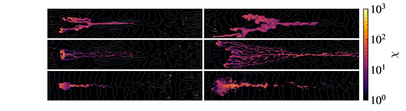
Figure 1: Morphology plots for simulations of $t_{\rm cool,mix}/t_{\rm cc}$$=0.1$ and $\beta=1,100$ and $10^{20}$ from top to bottom, respectively. Each figure represents a projection through the z-axis of overdensity $\chi$ at times $t=5,10\ t_{\rm cc}$ from left to right. Grey lines represent the contour lines for magnetic field lines in our runs. Earlier times exhibit higher compression of the lines near the cloud interface, shaping and draping overdense material under the influence of the wind.

2.3 Cloud tracking system

To minimise the amount of cold cloud material flowing outside the domain, we use a cloud-tracking system putatively described in Gronke & Oh (2018) (and in more depth in other studies e.g., Dutta & Sharma, 2019). We initially assign a passive, Lagrangian scalar concentration $C$=1 to the cold plasma (Xu & Stone, 1995). This variable is equally subject to the MHD equations via the influence of the MHD equations on the background gas velocity it advects with. From the mass continuity equation, it is possible to deduce the average cloud speed $u_{\rm cl}$:

$$\langle u_{\rm cl}\rangle=\frac{\int_{x_{\rm min}}^{x_{\rm cl,0}}u_{x}C_{\rm cl}\rho dV}{\int_{x_{\rm min}}^{x_{\rm cl,0}}C_{\rm cl}\rho dV}$$ (5)

$x$ is the coordinate basis for the wind speed direction, $x_{\rm cl,0}$ is the projected initial cloud centre position in the $x$-axis, $x_{\rm min}$ is the minimum $x$ value of the domain, $u_{x}$ is the velocity in the $x$-direction, $C_{\rm cl}$ is the initial maximum concentration of gas divided by three and $dV$ is the infinitesimal (cell) volume.

Similar to how it is described in previous work (Scannapieco & Brüggen, 2015; Brüggen & Scannapieco, 2016; McCourt et al., 2015; Farber & Gronke, 2022), this tracking method allows for a significant reduction in the box size required to contain the cloud material while reducing advection errors (Robertson et al., 2010).

3 Results

In this section we investigate the interplay between radiative cooling and magnetic fields (parametrized via $t_{\rm cool,mix}/t_{\rm cc}$ and $\beta$, respectively). We focus in particular on their impact on cloud gas survival.

3.1 Morphological Evolution

We begin by selecting simulations at fixed $t_{\rm cool,mix}/t_{\rm cc}=0.1$ to explore the dependence of the morphological evolution of clouds on relative magnetic field strength. In Figure 1 we display projections of the overdensity $\chi$ for $\beta=1,100\ \text{and}\ 10^{20}$ from top-bottom with dark regions of low overdensity and bright regions of high overdensity. We overplot magnetic field vectors as grey curves to explore the dependence of cloud morphology on relative magnetic field strength. The columns show different times in the evolution: $t=5,10\ t_{\rm cc}$ from left to right.

The left column shows snapshots at time $t=5t_{\rm cc}$. The top cloud corresponding to $\beta=1$ has a filamentary morphology with fairly weak magnetic fields outside the cloud but strong magnetic fields inside the filamentary cloud material. The second top row for $\beta=100$ shows the cloud has broken into several ‘head-tail’ structures which appear to be more ‘cored’ or chunky in the tail material; that is, the tail is not continuous cloud material. The magnetic field appears stronger over a wider area, corresponding to the greater lateral distribution of cloud material. In all cases of $\beta$ the magnetic field appears to be draping the cloud material.

The right column shows time $t=10t_{\rm cc}$. While the top row for $\beta=1$ again shows a single filament of cloud material, the second row from the top $\beta=100$ has a much broader lateral distribution of thin filaments looking like a spider’s web in morphology. For all three scenarios, Rayleigh-Taylor 3D instabilities are not suppressed under the influence of magnetic fields. This is in accordance to previous studies on magnetic RT instabilities (Stone & Gardiner, 2007b), suggesting that the nonlinear regime can even be amplified in the presence of magnetised gas. The bottom row still has strings of isolated cores of cloud material in contrast to the continuous filament in the top row. While all of these clouds survive, the rather different morphological evolution from the top row to the bottom rows suggests that cloud survival may be impacted by the morphological dependence on $\beta$.

3.2 Cloud Mass Evolution

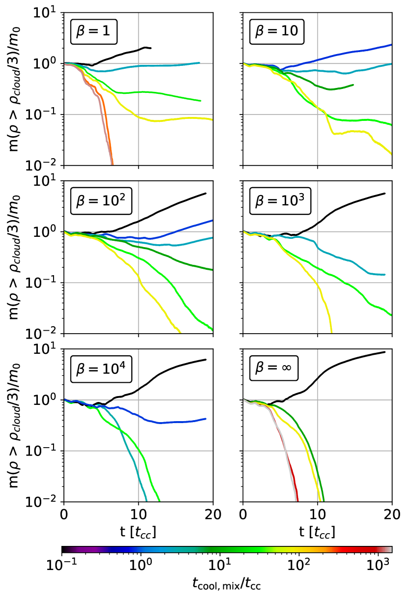
Figure 2: Cold gas mass evolution of clouds exposed to a $\mathcal{M}\sim 1.5$ wind and overdensity of $\chi\sim 100$ with different plasma $\beta$ (from $\beta\sim 1$ in the upper left to $\beta=\infty$ in the lower right panel) and varying cooling strength (indicated by the line color).

To further investigate the dependence of cloud survival on the interplay between radiative cooling ($t_{\rm cool,mix}/t_{\rm cc}$) and magnetic fields, we next explore the mass evolution of the full suite of simulations covering the $t_{\rm cool,mix}/t_{\rm cc}$-$\beta$ parameter range. Figure 2 shows the cloud gas, specifically $m(\rho>\rho_{\rm cloud}/3$), against time in units of $t_{\rm cc}$.

Each panel in Fig. 2 represents a different magnetic field strength with $\beta$=1, 10, 100, 1000, $10^{4}$, and $10^{20}$ ordered from top-left to bottom-right, respectively. In each panel we plotted the simulations performed at fixed $\beta$ and varying $t_{\rm cool,mix}/t_{\rm cc}$ (denoted via the color coding) to specifically determine the influence of $\beta$ on the critical $t_{\rm cool,mix}/t_{\rm cc}$ for survival of cloud material. The limiting cooling ratio for survival is expected to evolve with magnetic $\beta$. We selected $t_{\rm cool,mix}/t_{\rm cc}$ values that are inferred to lie closer to the survival limit for each $\beta$ case from neighbouring $\beta$ simulations, as opposed to performing them systematically for every possible $t_{\rm cool,mix}/t_{\rm cc}$, which would outstandingly increase the computational cost of finding the limiting criterion for each $\beta$.

The top-left panel of Fig. 2 displays simulations performed at fixed plasma beta of $\beta=1$ with five $t_{\rm cool,mix}/t_{\rm cc}$ values of 0.1, 3, 100, 300 and 1500. Interestingly, we find clouds survive (are destroyed) for $t_{\rm cool,mix}/t_{\rm cc}$ $\lesssim$ 100 ($\gtrsim$ 100), whereas hydrodynamic simulations find destruction for $t_{\rm cool,mix}/t_{\rm cc}$ $\gtrsim$ 1 (Gronke & Oh, 2018, and also the lower right panel of Fig. 2). Clouds with inefficient cooling ($t_{\rm cool,mix}/t_{\rm cc}$ $\gtrsim$ 100) display a rapid destruction. Clouds with efficient cooling, particularly, our run for $t_{\rm cool,mix}/t_{\rm cc}\sim 0.1$ exhibits an initial period of mass loss followed by mass growth. In the case of $t_{\rm cool,mix}/t_{\rm cc}\sim 3$, similar characteristics are observed, with the exception of apparent episodic saturation in growth of the cloud. These ‘bumps’ are not observed in previous works (Gronke & Oh, 2018) wherein once any evolving cloud begins growing in mass, the cloud continues growing in mass monotonically. These saturation interludes might be related to magnetic fields impacting the pulsations observed in earlier work. This may also be why $t_{\rm cool,mix}/t_{\rm cc}$ = 100 saturates at a reduced mass, as mass growth stagnates if there are no pulsations driving mixing. While oscillations in the mass loss rate can also be observed for dying clouds, the clouds are still rapidly destroyed.

Results for $\beta=10$ are shown in the top right panel of Fig. 2. Multiple runs were performed, varying $t_{\rm cool,mix}/t_{\rm cc}$ from 0.1 to 100. Growth in cloud material is observed for simulations with timescale ratios $\lesssim$ 10, contrasting with destroyed clouds for $t_{\rm cool,mix}/t_{\rm cc}=100$, and the $t_{\rm cool,mix}/t_{\rm cc}$ = 20 case was restarted several times but remains difficult to say if it will eventually lose all its dense gas or instead survive. For the $t_{\rm cool,mix}/t_{\rm cc}$ = 3 case, surviving gas experiences a critical point at $t\sim 13t_{\rm cc}$ in which it transitions from mass loss to growth. The aforementioned oscillatory behaviour in the mass curves can here be clearly noticed for $t_{\rm cool,mix}/t_{\rm cc}=100$, with ridges momentarily changing the tendency from mass loss to growth, yet the cloud still is ultimately destroyed.

The left-hand-side, second row panel shows the status for $\beta=100$ with $t_{\rm cool,mix}/t_{\rm cc}$ of 0.1, 1, 3, and 10 surviving, $t_{\rm cool,mix}/t_{\rm cc}$ $\sim$100 destroyed, and $t_{\rm cool,mix}/t_{\rm cc}$ = 30 which is again unclear despite several restarts.

The central right panel of Fig. 2 shows the runs with $\beta=1000$ for $t_{\rm cool,mix}/t_{\rm cc}$ values of 0.1 and 100. Here, the only surviving clouds are labelled as dark blue ($\beta=0.1$) and sky-blue ($t_{\rm cool,mix}/t_{\rm cc}=3$), while the dying clouds, yellow, corresponding to $t_{\rm cool,mix}/t_{\rm cc}=100$ and light-green ($t_{\rm cool,mix}/t_{\rm cc}$ = 30).

The bottom-left panel of Fig. 2, representing $\beta=10^{4}$, consists of runs with $t_{\rm cool,mix}/t_{\rm cc}=0.1,1,3$ and 30. The first two evidently survive, whereas the last two $t_{\rm cool,mix}/t_{\rm cc}=3$ and 30 are completely ablated by the hot gas. Sharper oscillatory behaviour is observed for this order of plasma beta values. Hence, for $\beta\sim 10^{4}$ we roughly recover the hydrodynamic survival criterion $t_{\rm cool,mix}/t_{\rm cc}$ $\lesssim 1$ (Gronke & Oh, 2018).

Lastly, the right-hand-side bottom panel of figure 2 displays simulations for $\beta=10^{20}$, serving for comparative purposes to hydrodynamic runs from Gronke & Oh (2018). The smooth dying nature of cold gas for $t_{\rm cool,mix}/t_{\rm cc}=3,100,1000$, and $10^{4}$ (green, yellow, red and silver) highly contrasts with the jagged mass increase of $t_{\rm cool,mix}/t_{\rm cc}=0.1$ (indigo), similar to the MHD runs. The destruction timescale for extremely weak cooling clouds are of similar duration, as are, although somewhat longer, for weak cooling $t_{\rm cool,mix}/t_{\rm cc}$ = 3 and 100.

Figure 2 demonstrates that the inclusion of magnetic fields increase the critical $t_{\rm cool,mix}/t_{\rm cc}$ value for cold gas survival dramatically at low $\beta$ and by a factor of a few even for as high $\beta$ as $\sim$10³. However, cloud destruction via Rayleigh-Taylor and Kelvin-Helmholtz instability cannot be completely suppressed, as we find destruction in all cases of $\beta$ we simulated for sufficiently large $t_{\rm cool,mix}/t_{\rm cc}$ (i.e., going towards the adiabatic limit). Note that Gronke & Oh (2020) found even adiabatic simulations of clouds survive, but only for low overdensities $\chi\lesssim 30$ (cf. Eq. 2), whereas we simulate high overdensities $\chi=100$. Although cold gas can die even at plasma beta $\beta$ values of 1, the critical $t_{\rm cool,mix}/t_{\rm cc}$ increases with decreasing $\beta$ suggesting a strong connection for survival between radiative cooling and magnetic fields, which we make more clear next.

3.3 Magnetic Fields Enhance Survival of Radiative Clouds

Figure 3 displays an overview of the $t_{\rm cool,mix}/t_{\rm cc}$-$\beta$ parameter space with the symbols indicating cloud survival or destruction clearly demonstrating that magnetic fields allow survival for less efficient radiative cooling than required in the hydrodynamic case (Gronke & Oh, 2018). In Fig. 3, clouds that are destroyed are represented by blue dots whereas for the case of survived, these are shown as orange squares. Information in the axis is in ordered, logarithmic scale, with $\beta$ varying from 1 to $10^{4}$ and a range of $t_{\rm cool,mix}/t_{\rm cc}$ scaling from 0.1 to 1500. Simulations with plasma beta of $10^{20}$, a numerical approximation to purely hydrodynamical scenarios, are excluded for ease of presentation.

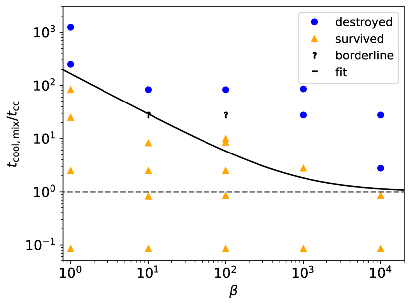
Figure 3: $t_{\rm cool,mix}/t_{\rm cc}$ against plasma $\beta$. The final state of the clouds are represented by blue dots in the case of survived, orange triangles for dissipated gas, black question marks for borderline cases, and we show the best fit powerlaw $t_{\rm cool,mix}/t_{\rm cc}=1.0+200\beta^{-0.7}$ as a black curve.

The curve delimiting the approximate boundary between destroyed and survived clouds $t_{\rm cool,mix}/t_{\rm cc}=1.0+200\beta^{-0.7}$ represents how the survival timescales of cold gas can vary as a function of plasma beta, $\beta$. Reading figure 3 from right to left in the plasma beta axis, i.e. coming down to lower betas from simulations nearer an ideal hydrodynamical scenario of $\beta=\infty$, reveals an upwards shift in the peaking timescales survival ratio of the clouds, becoming higher when approaching $\beta=1$.

For weak magnetic fields with $\beta=10^{4}$ we recover the hydrodynamical results with a critical $t_{\rm cool,mix}/t_{\rm cc}$ value of 1. Taking some distance from the hydrodynamic limit, for $\beta=10^{3}$, the critical time ratio for survival is $t_{\rm cool,mix}/t_{\rm cc}\sim 3$. Remarkably, for $\beta=1$, the critical $t_{\rm cool,mix}/t_{\rm cc}$allowing cold gas survival is approximately 100 times that predicted in the absence of magnetism, $t_{\rm cool,mix}/t_{\rm cc}\approx 1$ (Gronke & Oh, 2018). This case might be most relevant in the ISM where equipartition in thermal and magnetic energy densities is expected (Draine, 2011). We did not perform simulations below $\beta$ unity as these values are less relevant in galactic astrophysics (and numerically more challenging to evolve stably). In an attempt to better understand why magnetic fields produce such substantial changes in the survival criterion, we next turn to the entrainment time of these gas clouds.

3.4 Entrainment Time for Magnetized Clouds

An overview of the clouds’ velocity shear is represented in Figure 4. That is, we plot the time required for the cloud to reach half the wind velocity as a function of $\beta$. As previously, we plot surviving clouds as triangles and and destroyed clouds as circles, with colors representing the $t_{\rm cool,mix}/t_{\rm cc}$ ratio.

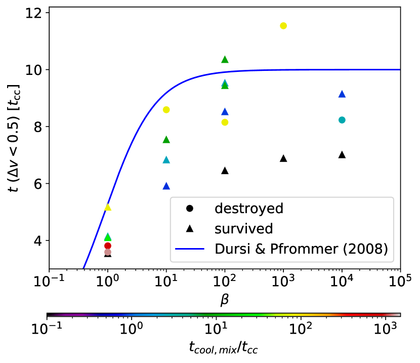
Figure 4: Time for the cold gas to reach $v=v_{\rm wind}/2$ vs $\beta$. Analogously to Figure 2, the value of $t_{\rm cool,mix}/t_{\rm cc}$is indicated by the colours of the symbols, and similar to Figure 3, we indicate clouds that survive as triangles and clouds that are destroyed as circles. The solid line shows the analytical estimate Eq. 1.

Figure 4 shows that the acceleration process depends strongly on the magnetization of the gas. Specifically, the entrainment time of the dense gas reaches its minimum for $\beta=1$, followed by a saturation for $\beta\gtrsim 10$ where $t_{\rm drag}\sim\chi^{1/2}t_{\rm cc}$ as expected from analytical theory (Dursi & Pfrommer, 2008).

While the trend is not monotonic, we do observe the fastest cooling runs show the most rapid entrainment, consistent with expectations since mass (and momentum) transfer $\dot{m}\propto t_{\rm cool}^{-1/4}$ (Gronke & Oh, 2020; Tan et al., 2021). Note, however, that this dependence is not very strong – and so the decrement in entrainment time is also not very large (i.e., two orders of magnitude change in cooling time only amounts to a factor of two reduction in the entrainment time).

Comparing the inefficient cooling cases, we find agreement with theoretical predictions from magnetic draping (cf. Eq. 1 Dursi & Pfrommer, 2008; Pfrommer & Dursi, 2010; McCourt et al., 2015; Sparre et al., 2020). The overall tendency matches the analytical prediction from equation  1, only displaying slight deviations of a few tcc due to the varying cooling efficiencies which, as aforementioned, has a minor impact on the entrainment time (see Appendix § B for an extended analysis). Yet the factor of two decrease in entrainment time does not evidently explain the $\sim$100 fold increase in survival for $\beta=1$ simulations and particularly not the $\sim$10 fold increase in survival for $\beta=100$ which is not appreciably accelerated faster than the hydrodynamic limit. To further explore what may bring about the increased survival for magnetized clouds we next investigate the mass accretion rate dependence on $\beta$ to investigate possible suppression of mixing by magnetic fields.

3.5 Mass Accretion Rate

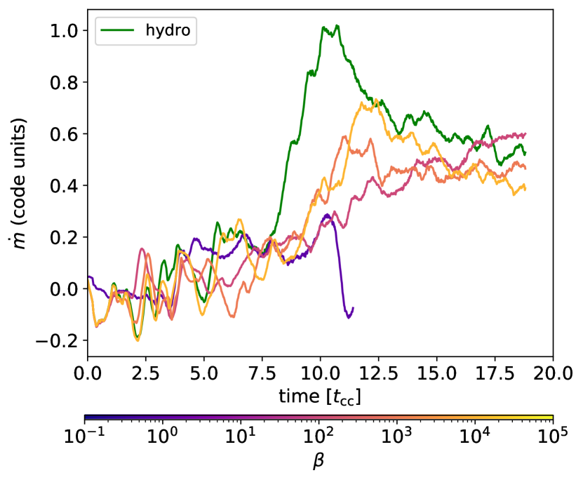
Figure 5: Mass growth rate of clouds (defined as material with $\rho>\rho_{\rm cl}/3$) as a function of time for a fixed $t_{\rm cool,mix}/t_{\rm cc}=0.1$ and varying $\beta$ (a hydro run is the green line for comparison).

In Figure 5, we show the mass accretion rate against the time elapsed in units of $t_{\rm cc}$. We aim to explore how varying $\beta$ conditions may modify gas accretion from hydrodynamic instabilities, for which a fixed $t_{\rm cool,mix}/t_{\rm cc}$ ratio of 0.1, observed to survive regardless of plasma beta, is chosen as value of reference. We indicate $\beta$ by colours as previously and include a hydro run as a green curve for comparison purposes.

The overall picture reveals that $\dot{m}$ is fairly insensitive to $\beta$ with the mass growth in the hydrodynamical simulation maximally a factor of $\sim 10$ larger than in the low $\beta$ run and a factor of a few larger than high $\beta$ runs, but most of the time only tens of percent difference. This is somewhat surprising as linear analysis and shearing box simulations show that mixing is suppressed (after magnetic fields amplify and possibly the turbulent velocity has diminished) even with initially weak magnetic fields (Ji et al., 2018; Grønnow et al., 2022) – but consistent with a previous study (Gronke & Oh, 2020).

4 Discussion.

4.1 The survival of cold gas in magnetized galactic winds

Our findings show that the combination of radiative cooling and magnetic fields allows $T\sim 10^{4}\,$K cold gas to survive in a hot ($T\sim 10^{6}\,$K) wind if

$${t_{\rm cool,mix}/t_{\rm cc}}\lesssim\frac{200}{\beta^{0.7}}\ +1.$$ (6)

This implies that the physical parameter space for survival is increased drastically which is clear when rewriting Eq. (6) to a geometrical criterion yielding

$$r_{\rm cl}\gtrsim R_{\rm crit,cl}\sim 2\textrm{\,pc}\frac{T_{cl,4}^{5/2}\mathcal{M}}{P_{3}\Lambda_{\rm mix,-21.4}}\textrm{min}\left(1,\frac{\beta^{0.7}}{200}\right).$$ (7)

Here, $T_{\rm cl,4}\equiv T/(10^{4}\,{\rm K})$ is the cloud temperature in units of $10^{4}$ K, $\mathcal{M}$ is the Mach number, $P_{3}\equiv P/(10^{3}\,{\rm cm}^{-3}\,\rm{K}$) is the pressure (per Boltzmann constant) in units of $10^{3}$ cm^-3 K, $\Lambda_{\rm mix,-21.4}$ is the cooling rate in units of $10^{-21.4}$ erg cm³ s^-1, and the last term includes the effects of magnetic fields, which impact the survival when $\beta\lesssim 10^{4}$.

This strong effect on the survival criterion might be surprising given our other results:

1. While magnetic fields aid in cloud entrainment this effect is only $\mathcal{O}(1)$ (cf. Fig. 3 and Eq. 1), i.e., at first sight too weak to explain the $\sim 2$ order of magnitude change in survival criterion for $\beta\sim 1$.

2. Similarly, one expects magnetic fields to suppress turbulence and hence inhibit mixing. However, contrasting the evolution of the turbulent velocity, measured as the velocity orthogonal to the wind axis, for various selections of data ($\rho>\rho_{\rm cl}/3$, $T<2T_{\rm fl}$, and $T<T_{\rm mix}$) revealed no significant differences between simulations with magnetic fields compared to hydrodynamic cases (see Appendix § C).

3. We also checked if other effects such as compression due to magnetic fields and hence a lowered $t_{\rm cool}$ play a role but only found a small ($\lesssim$ factor of a few) change for relatively short durations ($\sim$1 - 2 $t_{\rm cc}$). Since we expect the mass growth of the cold medium $\dot{m}\propto t_{\rm cool}^{-1/4}$ (Gronke & Oh, 2020; Tan et al., 2021; Fielding et al., 2020) or at most $\dot{m}\propto t_{\rm cool}^{-1/2}$ (Ji et al., 2018; Tan et al., 2021), we consider this effect to be negligible.

4. We do not find large changes in the mass evolution of cloud material when including magnetic fields. This is suggested by Fig. 2 when comparing the mass evolution for runs with weak cooling. For instance, independent of $\beta$, the ${t_{\rm cool,mix}/t_{\rm cc}}\sim 10^{3}$ simulations lose all cloud mass by $t\sim 8t_{\rm cc}$. This is also consistent with the fact that we observe similar mass growth (and thus mixing) rate for the low-$\beta$ runs in Fig. 5 for most of the time evolution, amounting to at most a factor of 2 suppression in mass growth when including magnetic fields compared to the hydrodynamic case in Fig. 2. However, note that these are limiting cases – either specific times or very weak cooling – and thus less relevant to the survival threshold which is (per definition) a limiting case.

In summary, we have found two effects clearly altered by the presence of magnetic fields: the acceleration process and the mass evolution (discussed in 1 and 4 above, respectively). However, both of these effects are seem rather weak and not sufficient to explain the large change in the survival threshold. Below, we will analyze both effects in more detail.

First, we focus on these effects in the weak / no cooling limit. Fig. 6 shows the mass and velocity evolution for very weak and no cooling cases contrasting the pure hydrodynamical and $\beta\sim 1$ runs. Clearly, magnetic fields do speed up entrainment (cf. §3.4) but do not prolong the destruction process. Only with ${t_{\rm cool,mix}/t_{\rm cc}}\sim 100$ (red curve in Fig. 6) the mass evolution is clearly altered. Notice that discontinuities in entrainment curves are a direct consequence of our cold gas criterion: for some time intervals, overdense gas can become diffuse enough not to satisfy the $m(\rho>\rho_{\rm cl}/3)$ condition. This appears as gaps in the velocity shear tendency. As it progressively accretes gas from the medium, it can make the cut and be displayed in the figure again.

The situation is, however, different with more efficient cooling. In Fig. 7, we show the cloud mass evolution normalized by the hydrodynamic run’s mass and additionally show the relative velocity evolution in Fig. 7, for the case of $t_{\rm cool,mix}/t_{\rm cc}$ = 0.1. Even while the $\beta=10^{4}$ simulation (orange curve in Fig. 7) is entrained only slightly slower than the hydrodynamic case, it has a reduced mass compared to the hydrodynamic case, suggesting magnetic fields do suppress mixing, if marginally in these cases.

Figure 7, also shows that for $\beta=1$ the relative velocity not only drops to $\sim$half its initial value but is a factor of $\sim$5-10 lower at 8 cloud crushing times than the hydrodynamic case, which is when clouds were destroyed in the limit of weak cooling cases. Furthermore, at later times ($t\gtrsim 10t_{\rm cc}$), the entrainment is faster also for $\beta=10$ although this is not expected from draping which should play a negligible role for $\beta\gtrsim 10$ (Eq. 1).

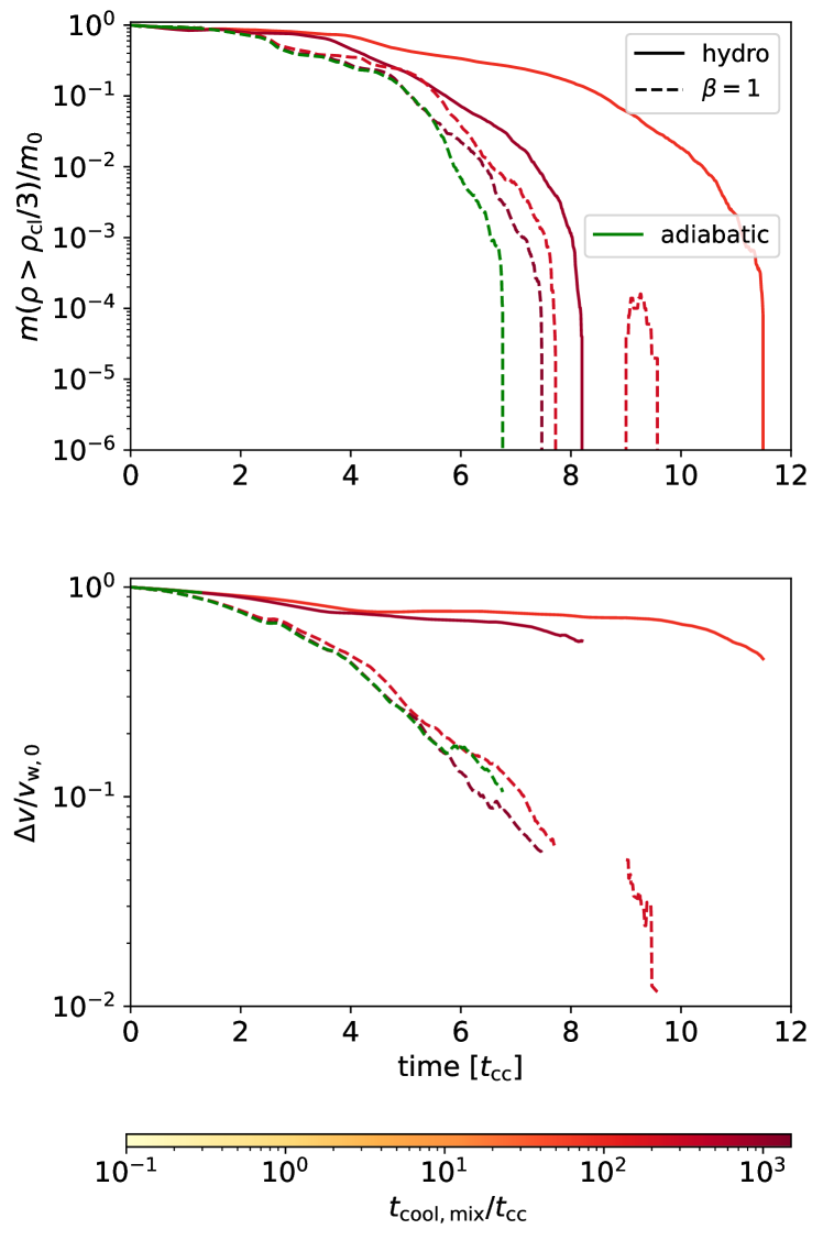
Figure 6: Time evolution of the mass (top panel) and relative velocity between the wind and cloud (bottom panel) for clouds which are destroyed in hydrodynamic runs and $\beta=1$ as solid and dashed curves respectively, as a function of $t_{\rm cool,mix}/t_{\rm cc}$ (note that we mark the adiabatic runs as green and the we changed colormaps since otherwise the adiabatic run may lead to confusion).

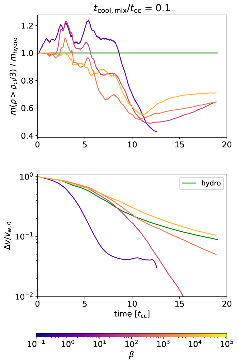
Figure 7: Time evolution of (top panel) the cloud mass normalized to the cloud mass in the hydrodynamic case (hence, the green curve is flat and has a value of unity throughout) and (bottom panel) the relative velocity between the cloud material and hot wind ($\Delta v)$ normalized to the initial wind velocity ($v_{\rm w,0}$).

To further investigate the ability of magnetic fields to aid cloud survival we show in Fig. 8 time series of cloud mass (top panel), relative velocity (middle panel), and scalar concentration (bottom panel, see Methods 2.3) for $t_{\rm cool,mix}/t_{\rm cc}$ = 100, since with this cooling efficiency only the strongly magnetized case $\beta=1$ survives. Even with magnetic fields as weak as $\beta=10^{3}$, the lifetime of the cloud is extended by a few cloud crushing times and lower $\beta$ cases take about twice as long as the hydrodynamic case before they are destroyed. Although $\beta=1$ and $10$ are completely entrained, with $\Delta v/v_{\rm w,0}<10^{-4}$, they still have substantial values of their scalar fields, demonstrating entrainment occurs in these cases before the original cloud material is fully mixed.

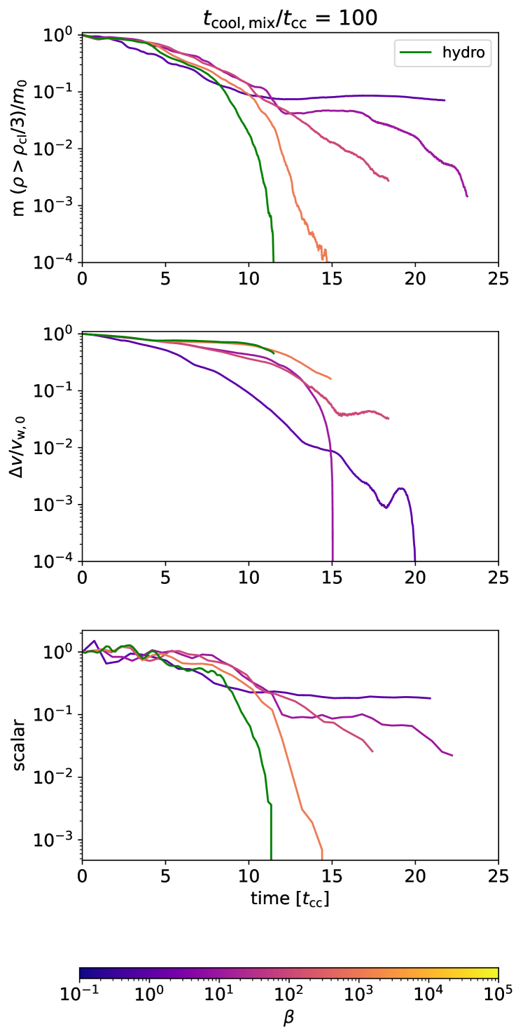
Figure 8: Time evolution of the mass (top panel), relative velocity between the wind and cloud (middle panel), and Lagrangian scalar concentration initially assigned to cold gas (bottom panel) for $t_{\rm cool,mix}/t_{\rm cc}=100$ as a function of $\beta$ (with the green curve indicating a hydro run for comparison). From this plot, it is clear that lower $\beta$ clouds survive (longer) because they entrain more quickly and mix less / more slowly.

To summarize: Why does the cold gas survival criterion change by orders of magnitude although the individual MHD effects are rather small? First, recall that we only require $t_{\rm drag}\lesssim\chi^{1/2}t_{\rm cc}$, that is, nominally a reduction of $t_{\rm drag}$ by a small amount for $\chi\sim 100$ to allow for $r_{\rm crit}\rightarrow 0$ (recall $t_{\rm drag}$ scales linearly with $\chi$ so changing $\chi$ by e.g., 4 reduces the drag time by a factor of 4, but the cloud crushing time by only a factor of 2). As mentioned above, Gronke & Oh (2020) found a critical $\chi\sim 30$ below which clouds were entrained before they were destroyed in even adiabatic simulations. This implies a disproportionally large change in the critical $t_{\rm cool,mix}/t_{\rm cc}$-criterion is possible for a small change in $t_{\rm drag}$ for $\chi=100$.

In other words, the question boils down to: Why do magnetic fields cause faster entrainment? First, there is the ‘draping effect’ discussed in § 1. However, we also demonstrated that with cooling, the entrainment process is faster than expected from draping alone (cf. Fig. 4). To understand this, recall that the drag time $t_{\rm drag}\propto\chi$. Therefore, if magnetic pressure supports more tenuous material than would be stable in thermal pressure equilibrium, then acceleration can occur more rapidly. In Fig. 9 we show the time evolution of the overdensity $\chi$, including simulations with $\chi=10^{3}$. The case that clearly survives ($t_{\rm cool,mix}/t_{\rm cc}$ = 5, the darkest green curve) has the largest decrement in $\chi$ by a factor of $\sim$5, whereas somewhat more inefficient cooling cases ($t_{\rm cool,mix}/t_{\rm cc}$ = 30 and 50) only have $\chi$ drop a factor of $\sim$3 and are marginally destroyed or marginally survive (in the $t_{\rm cool,mix}/t_{\rm cc}$ = 50 case, the cloud mass drops slightly below 1% just as the relative velocity is dropping below 1% after which it might grow at the end of the simulation). The $\chi=10^{3}$ case which was clearly destroyed ($t_{\rm cool,mix}/t_{\rm cc}$ = 500, red curve) interestingly does not drop in overdensity until it is completely mixed away. This suggests more efficient cooling entrains magnetic fields more effectively which are amplified as they are compressed, providing nonthermal pressure support and reducing the average overdensity. Note that while the hydrodynamic case regains thermal pressure equilibrium and $\chi$ returns to its initial value, the average overdensity remains lower in the cases with magnetic fields. Hence, the entrainment process even for larger $\beta$ is accelerated – more than expected from pure ‘draping’. This leads to comoving (and thus surviving) cold gas and is therefore the main effect for the change in survival criterion found. This point is further discussed in Appendix § D.

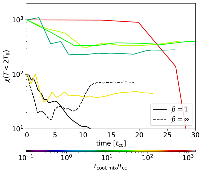
Figure 9: Time evolution of the density ratio $\chi$ between hot tenuous wind and cold dense ‘cloud’ material. In this case we use $T<2T_{\rm fl}$ to define ‘cloud’ material but note that the result is very similar for $\rho>\rho_{\rm cl}/3$. The black dashed curve is a hydrodynamic case with $t_{\rm cool,mix}/t_{\rm cc}=1$ and an initial $\chi=100$ for reference, and note we include runs with initial $\chi=100$ and $\chi=1000$ as should be evident by their value at time = 0 $t_{\rm cc}$. While the hydrodynamic case loses initial thermal pressure equilibrium, it re-establishes its initial overdensity at $\sim 10t_{\rm cc}$. In contrast, all cases with magnetic fields (except the red curve corresponding to $t_{\rm cool,mix}/t_{\rm cc}=500$ which is destroyed) maintain a factor of few suppression to their initial overdensity, suggesting magnetic pressure support plays a role in their evolution.

4.2 Comparison to Previous Work

We next discuss how our results compare to previous work. One of our most staggering results is the finding that significantly smaller clouds $t_{\rm cool,mix}/t_{\rm cc}\sim 100$ can survive under conditions of low $\beta$ compared to $t_{\rm cool,mix}/t_{\rm cc}\sim 1$ in the hydrodynamical case.

While many previous studies (e.g., Gregori et al., 1999; Banda-Barragán et al., 2016; Grønnow et al., 2018) included magnetic fields in wind-tunnel simulations, there has been no consensus of whether magnetic fields aid survival and under which conditions. Gregori et al. (1999), for instance, concluded that magnetic fields lead to a faster destruction due to faster acceleration and, thus, a shorter Rayleigh-Taylor timescale. In contrast, McCourt et al. (2015) show that cold gas can survive when including magnetic fields. However, they focus on moderate overdensitites of $\chi\sim 50$ and include radiative cooling. Since McCourt et al. (2015) include radiative cooling, it is possible that their simulations effectively fall under the critical $\chi\lesssim 30$ (cf. Eq. 2).

Li et al. (2020) carried out a large suite of simulations which also include magnetic fields. They found an alternative survival criterion to Gronke & Oh (2018) used here which compared the hot gas cooling time $t_{\rm cool,hot}$ to an empirically calibrated survival time $t_{\rm life}$ (see Kanjilal et al., 2021, for a discussion and comparison of the criteria in the hydrodynamic case). Interestingly, the magnetic field does not enter $t_{\rm life}$ and thus the survival criterion of Li et al. (2020) appears at odds with our findings. However, they focus mainly on the $\beta=10^{6}$ parameter space where we find the effect to be negligible. Noteworthy, Li et al. (2020) additionally included anisotropic conduction and viscosity which complicates comparison.

(Sparre et al., 2020) perform cloud crushing simulations with magnetic fields focusing on the $\beta\geq 10$ case, and in particular on the hydrodynamic case. They do find enhanced cloud survival including magnetic fields – for example, their $R_{\rm cl}=15$ pc cloud survives in their Figure A2 including magnetic fields whereas the same cloud is destroyed in their hydrodynamic run, shown in their Figure D1 – without discussing the effects of $B$-fields systematically.

Cottle et al. (2020) performed three-dimensional cloud-crushing simulations with $\chi=10^{3}$, $\mathcal{M}=3.5$, and $\beta=10$ (and two cases with $\beta=1$), comparing wind axis-aligned magnetic fields to transverse magnetic fields. They found shock-aligned magnetic fields increase the mixing rate by a factor of a few whereas transverse fields drape and pinch clouds leading to a wider perpendicular distribution of cloud material and rapid mass loss. Interestingly, Cottle et al. (2020) claim destruction for their simulations even in a very efficiently cooling regime $t_{\rm cool}/t_{\rm cc}=10^{-6}$, although presumably they evaluated the cooling time at $T_{\rm cl}$ since we find for their parameters $t_{\rm cool,mix}/t_{\rm cc}\sim 0.1$. Also note they use the Wiersma et al. (2009) cooling curve whereas we use Sutherland & Dopita (1993) and thus their cooling rate is $\sim$2 lower at $T_{\rm mix}$ and perhaps more significantly their integrated cooling rate below $T_{\rm mix}$ may be substantially reduced compared to ours (see Wiersma et al. 2009, their Figure 1 for a comparison of the cooling curves; also interestingly, their integrated cooling time is longer than ours above $T_{\rm mix}$). Nevertheless, one might expect a different outcome in their case since their $\mathcal{M}=3.5$ is larger than the transonic case studied here.

We do not attempt a full comparison but conclude by noting we consider our studies complementary since we study the transonic case $\mathcal{M}=1.5$ whereas Cottle et al. (2020) consider the supersonic scenario $\mathcal{M}=3.5$.

Regarding morphology of the cold gas, our findings agree with previous studies. For instance, in agreement with Ruszkowski et al. (2014) we find hydrodynamic simulations have more discontinuous cores whereas magnetized wind-tunnel simulations have a more filamentary, contiguous morphology (among many others, also see Tonnesen & Bryan, 2010; Tonnesen & Stone, 2014; Jung et al., 2022).

4.3 Implications for Observations

Both absorption and emission measurements commonly detect cold $10^{4}$ K gas in the circumgalactic medium of objects with virial temperature being $T_{\rm vir}\sim GM/R\sim 10^{6}$ K as confirmed in soft X-ray observations (Tumlinson et al., 2017) (although there may additionally be a $10^{7}$ K phase; Gupta et al. 2021). A wide variety of circumgalactic medium observations suggest this cold gas has a scale as small as $\sim$pc (as reviewed in McCourt et al. 2018). In addition, detections of rapidly outflowing cold gas in galactic winds close to the expected launching radius of the wind suggest rapid acceleration (Veilleux et al., 2020), and we find magnetic fields induce rapid acceleration even for clouds that are destroyed (recall Fig. 6).

Our results of magnetic-draping enhanced acceleration and low $\beta$ enhanced survival of cold gas shifts the previous survival criterion – and thus the size of survivable clouds – by orders of magnitude. This may thus help to explain observations of rapidly outflowing cold clouds and small-scale cold gas in the circumgalactic medium. Moreover, our findings suggest that if the accelerated clouds have dynamically important magnetic fields, observations should seek sub-pc clouds, which may be discovered by future deep HI observations such as with ASKAP (Dickey et al., 2013), JVLA (Murthy et al., 2021), MeerKAT (Pourtsidou, 2017), or other observatories.

Moreover, our simulations may help to explain the cold gas observed in the tails of jellyfish galaxies that form when late-type spirals are subjected to ram pressure from high-pressure intracluster media (most spectacularly, the $\sim$60 kpc star-forming tail of D100 in Coma, Cramer et al. 2019 but see Poggianti et al. 2017 for additional examples from the GASP survey). Simulations of jellyfish galaxies find that dense gas is difficult to strip (Tonnesen & Bryan, 2012) but stripped gas clouds may evolve due to mixing with the ambient intracluster medium (Tonnesen & Bryan, 2010, 2021). Our results suggest including magnetic fields in future simulations of jellyfish galaxies may allow smaller clouds to grow.

Another important observational implication is the strong magnetic pressure support and the consequent lower overdensitites found (cf. Fig. 9). This effect might explain cold gas found to be out of (thermal) pressure equilibrium in the CGM (Werk et al., 2014).

4.4 Caveats

• Resolution: fiducial values are set to a fixed resolution $r_{\rm cl}/d_{\rm cell}=16$ to permit a wide parameter sweep of $\beta$ and $t_{\rm cool,mix}/t_{\rm cc}$. Previous simulations find this resolution is adequate for converged mass growth (Gronke & Oh, 2020; Tan et al., 2021). A test of numerical convergence is shown in Appendix § A.

• Numerical limitations: The cloud-tracking system aims to avoid gas outflows of the simulation domain, enabling the use of a reduced 3D box-size. Nevertheless, $\beta=1$ simulations exhibit a substantial expansion of cloud material orthogonal to the wind axis (as seen by several previous studies such as Cottle et al. 2020) which required larger box sizes and hence costlier simulations. Additionally, $\beta=1$ and $\chi=10^{3}$ simulations were numerically unstable at late times (omitted from our analysis) which made it difficult to definitively assess whether borderline clouds would end up being destroyed or survive if we could stably evolve our simulations longer. Future simulations utilizing a more stable Riemann solver such as HLL3R (Waagan et al., 2011) or otherwise more stable numerical methods may help us study lower $\beta$ and higher $\chi$ evolved to longer times.

• Initial parameters: we performed our simulations primarily at $\chi=100$ yet clouds likely span overdensities of $10^{2-4}$ (that is, they exist in pressure equilibrium, such as $10^{4}$ K gas in the $10^{8}$ K intracluster medium). Note however that higher overdensities are more numerically expensive and we wished to run a wide sampling of simulations to elucidate clearly the impact of radiative cooling and magnetic fields on cloud survival. Moreover, we only ran simulations at $\beta_{\rm wind}=\beta_{\rm cl}$ whereas in reality these values may likely be different. However, Gronke & Oh (2020) studied independently varying $\beta_{\rm cl}$ and $\beta_{\rm wind}$ and found $\beta_{\rm wind}$ was the most determining parameter, so we do not expect significant modifications to our results. Furthermore, we only explored transonic $\mathcal{M}=1.5$ winds. Such are expected to be relevant to the conditions of the launching radius of galactic winds (Chevalier & Clegg, 1985); however, if clouds are sourced from the CGM at greater distances from the base of the galactic wind, exploring higher Mach numbers would be more relevant. We leave such exploration to future work and refer the reader to Sparre et al. (2020) for the case with $\beta=10$ who studied $\mathcal{M}=4.5,1.5$ and 0.5 and Cottle et al. (2020) for cases of $\beta=10$ and 1 with $\mathcal{M}=3.5$.

• Interplay of complex dynamical processes: Pressure-driven fragmentation of clouds undergoing thermal instability as they are subjected to a hot wind has not been studied in this work, but would be an interesting avenue for future research. Furthermore, we neglected potentially important physical processes such as conduction, viscosity, turbulence, and cosmic rays which may impact our results. We plan to study these effects in future work. Recently, Brüggen et al. (2023) have conducted a study focusing on the problem of thermal conduction and its impact on cloud survival in combination with magnetic fields.

5 Conclusions.

We perform simulations of radiative cold magnetized clouds subject to hot magnetized winds. We ran simulations with $\beta=1,10,100,10^{4},$ and $10^{20}$ (hydrodynamic limit) each with various $t_{\rm cool,mix}/t_{\rm cc}$ from 0.1 to $10^{4}$. Introducing strong magnetic fields in such plasmas favours their survival for a critical $t_{\rm cool,mix}/t_{\rm cc}$ 100 fold above the hydrodynamical scenario in conditions of low $\beta\sim 1$ and 10 fold for $\beta\sim 10$ (cf. Eqns. 6 & 7 for a cold gas survival criterion in a magnetized wind). For $\beta\gtrsim 10^{4}$ we recover the hydrodynamical survival criterion.

As most astrophysical plasmas are magnetized, this implies that much smaller clouds can survive ram pressure acceleration than previously thought. We attribute this strong impact to a more rapid entrainment process leading to an entrainment time shorter than the cloud’s destruction time. We find that this rapid entrainment cannot be explained by magnetic draping alone but is also due to a lower cold gas overdensity (and hence faster acceleration since $t_{\rm drag}\propto\chi$) caused by non-thermal pressure support because of compressed magnetic fields. In summary, we find that the key aspect is the interplay of magnetic field lines and cooling which has a combined much stronger effect than the individual components themselves.

Other results of our work are in broad agreement with previous publications on cold magnetized cloud survival that generally find enhanced cloud survival when including radiative cooling and magnetic fields, as well as simulations that find enhanced destruction in adiabatic simulations with magnetic fields. We find magnetic fields do not completely arrest Kelvin-Helmholtz instability except possibly at late times in cases of efficient cooling and $\beta=1$ as well as cases with weak but non-negligible cooling $t_{\rm cool,mix}/t_{\rm cc}=100$ with $\beta=1$.

The rates of cold mass growth in MHD scenarios appear to coincide with past and simulated hydrodynamical cases for the same initial parameters, reaching constant stable growth at late stages, except a slight suppression of growth for $\beta=1$.

While our simulations help to understand the evolution and survival of cold gas in hot winds, our results have certain limitations related to the restricted range of parameters we explored. Supersonic Mach numbers, higher overdensities, turbulence, conduction, viscosity, cosmic rays, and perhaps radiation pressure may have an impact on our results. In the future, we would like to extend this work for a larger parameter range to determine the impact this may have on the now more-advanced, classical cloud survival problem.

Data Availability

Data to confirm the results of this work will be shared upon reasonable request to the authors.

Appendix A Numerical convergence

Previous work has shown that even at resolution as low as 8 cell lengths per cloud radius leads to convergence in mass evolution and growth Gronke & Oh (2020). In short, this is because the mixing time $t_{\rm eddy}\propto l^{2/3}$, i.e., increases with scale. In other words, the factor limiting mixing is the large eddies which we are resolving (Tan et al., 2021). For our systematic study of magnetised plasmas, we employ a cell length/cloud radius ratio of 16. Using the fiducial run of initial values $\beta=1$, $t_{\rm cool,mix}/t_{\rm cc}$ = 0.1, we contrast our simulation with the produced mass evolution for a cold cloud of resolutions $r_{\rm cl}/d_{\rm cell}=32$.

These two resolutions displayed in 10, represented by the solid-blue and dashed-orange lines, respectively, exhibit only minute deviations of order $\mathcal{O}{(}{-1)}$ at $\sim$7 $t_{\rm cc}$, demonstrating similar behaviour for both resolutions.

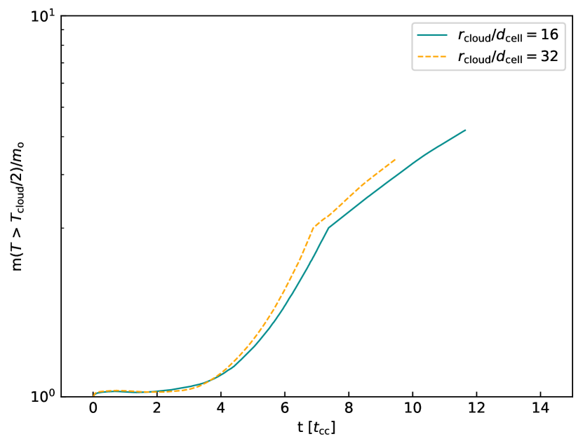
Figure 10: Runs for initial conditions $\beta=1$, $t_{\rm cool,mix}/t_{\rm cc}$ = 0.1 employing resolutions of $r_{\rm cl}/d_{\rm cell}=32$ (dashed-orange) and $r_{\rm cl}/d_{\rm cell}=16$ (solid-blue), respectively. Further comparative analysis for different resolutions can be compared in Gronke & Oh (2020).

Appendix B Shear evolution

The entrainment of cold gas through momentum transfer from the hot wind to the cloud is an important element in solving the cloud crushing problem. Figure 11 shows the evolution of the velocity difference between the hot and the cold medium for a variety of our runs.

In the y-axis, we plot the shear velocity of the cloud with respect to the wind, normalised to the initial wind speed and thus 1.0 represents a static cloud and 0 indicates full entrainment by the wind. The evolution of velocities is displayed in cloud crushing timescales, $t_{\rm cc}$. Cooling efficiencies are encoded by the bottom colourbar. Significant variations in curve steepness can only be seen for low betas, more specifically, for $\beta=1$.

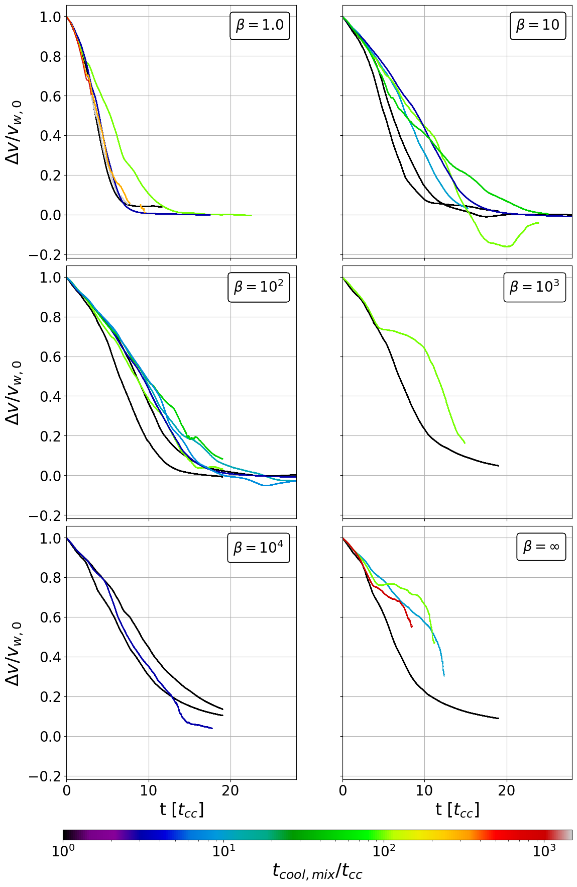
Figure 11: Evolution of the shear between cold gas and a $\mathcal{M}\sim 1.5$ hot wind with an overdensity of $\chi\sim 100$. We vary $\beta$ (from $\beta\sim 1$ in the upper left to $\beta=\infty$ in the lower right panel) and cooling strength (indicated by the line color).

Figure 12 shows multiple versions of figure 4 with varying "entrainment time", defined as the time when the shear velocity drops below a certain threshold. A faster rate in cloud acceleration appears to be related to faster cooling efficiencies for the clouds (at fixed $\beta$), expressed in terms of $t_{\rm cool,mix}/t_{\rm cc}$ and which is mapped accordingly to the bottom colourbar. Overall, moving to the right in the x-axis displays a $\sim$ few fold increase in entrainment time as a function of $\beta$, recovering the fiducial timescales from figure 4 as we move upwards to the top subplot.

Note that, although destroyed clouds might be expected to entrain later than survived clouds, some datapoints reveal the opposite (e.g. $t_{\rm cool,mix}/t_{\rm cc}=300$ for $\beta=1$). However, we observe the cold gas for these cases to get destroyed before entraining to lower shear values (e.g. $\Delta v<0.01$), which suggests that the final stages of entrainment can be decisive in the final fate of the cloud.

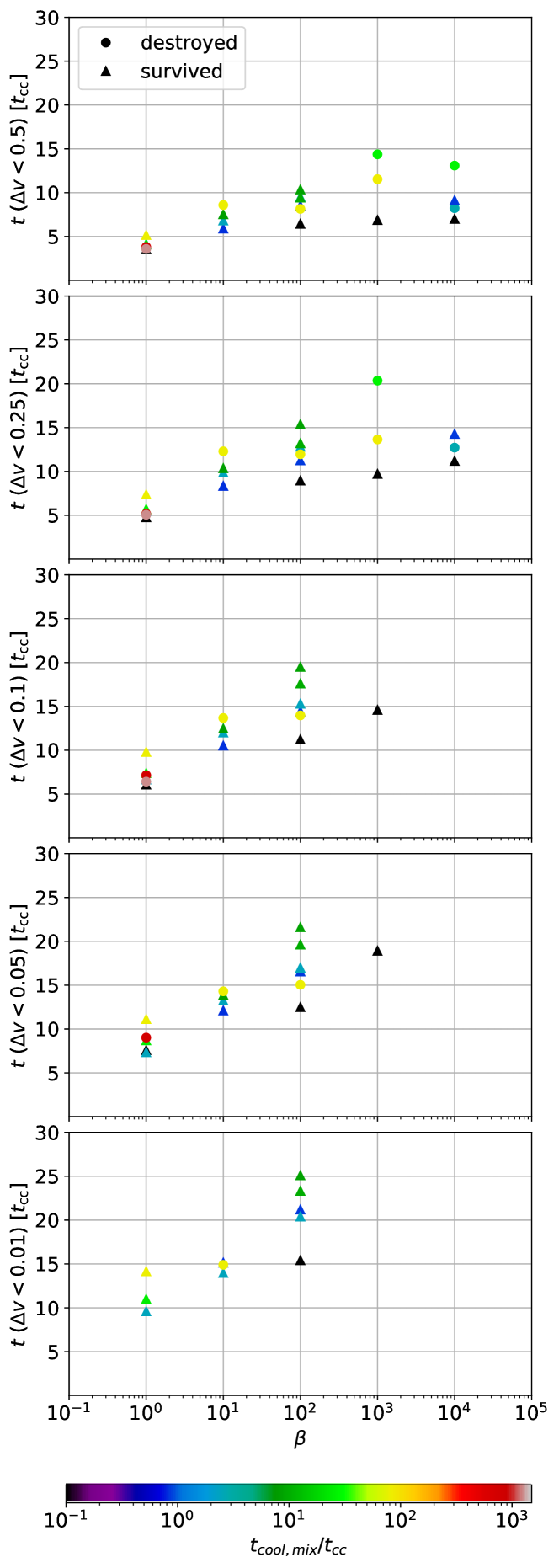
Figure 12: Time for cloud material to be ‘entrained’ ($\Delta v<\alpha$ for thresholds from $\alpha=0.5$ (top) to $\alpha=0.01$ (bottom)). Note that in many of our simulations, clouds are completely destroyed or are already evidently growing (at which point we stop restarting them) by $\Delta v<0.01$ or even $\Delta v<0.1$. One would expect that clouds that survive entrain faster than clouds that are destroyed. However, we observe several exceptions to this expected trend, particularly at $\beta=1$ in which case $t_{\rm cool,mix}/t_{\rm cc}=300$ (red circle, which is destroyed) entrains even to $\Delta v<0.05$ faster than $t_{\rm cool,mix}/t_{\rm cc}=100$ (yellow triangle, which survives). However, $t_{\rm cool,mix}/t_{\rm cc}=300$ is destroyed before entraining to $\Delta v<0.01$ suggesting the last 10% of the entrainment (which requires 1.5 - 2.5 $t_{\rm drag}$ is critical for cloud survival.

Appendix C Turbulence suppression

The influence of magnetic fields on hydrodynamical instabilities such as Rayleigh-Taylor or Kelvin-Helmholtz is an on-going topic of discussion in the literature (e.g., bubbles; Fielding et al., 2020). In figure  13, we study this problem in more detail by showing the evolution of the mass-weighted, geometric-mean velocity of cold gas orthogonal to the direction of the wind. The velocity is expressed as a fraction of the sound speed of gas at $T_{\rm cl}$, i.e. $v_{\rm rms}/c_{\rm s,cold}$, where $c_{\rm s,cold}$ represents the sound speed of the cold phase.

Broadly, the speed decreases slightly once the wind encounters the cloud, and only exhibits a small deviation in late-time behaviour with respect to the general trend for the case of $\beta=1$. As discussed in § 4, simulations experience similar features in turbulence both under the presence of magnetised plasmas and without them. On average, we observe that late time $v_{\rm rms}/c_{\rm s,cold}$ tend to unity, only varying by a factor of $\sim$ few. Such a level of late time turbulence is expected from pulsations of the cloud; that is, we previously found late time turbulence is not shear-driven (Gronke & Oh, 2020; gronke2023; Abruzzo et al., 2022).

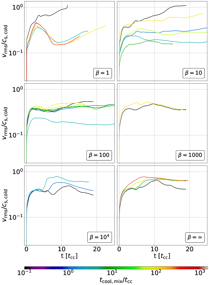
Figure 13: Mass-weighted root-mean-square velocity of the speed components orthogonal to the wind. As discussed in § 4.1 and Appendix C, magnetic fields have a small effect on the turbulent velocity.

Appendix D Internal plasma beta evolution

In § 4.1 (cf. Fig.  9), we argue that magnetic pressure support accounts for the drop in late-time cloud overdensities in scenarios where $\beta$ is close to unity. This contrasts with purely hydrodynamical simulations, where overdensities $\chi$ recover their initial values after a few $t_{\rm cc}$. Figure 14, representing the internal magnetic field evolution of cold gas, shows direct evidence of the existence of significant magnetic pressure in the late-time evolution, supporting the hypothesis that magnetic fields can support this difference in overdensities. Specifically, we computed $\beta=P_{\rm gas}/P_{\rm B}$ via an ideal gas equation of state for $P_{\rm gas}$ and $P_{\rm B}=B^{2}/(8\pi)$. We restricted our computation of $\beta$ to cells satisfying $T<2T_{\rm min}$ and plot the median value at each time. Notice that $T_{\rm min}$ represents the floor temperature of the simulation.

The plot studies the evolution of plasma beta, $\beta$, for runs of ${t_{\rm cool,mix}/t_{\rm cc}}=0.1$ and various initial betas (purple, $\beta=10^{4}$; red, $\beta=10^{3}$ ;green, $\beta=10^{2}$; orange, $\beta=10$; blue, $\beta=1$). Our results suggest cold gas exhibits values $\sim$few, regardless of the initial $\beta$. This is in agreement with previous studies which show a similar enhancement in magnetic field strength in a cooling, multiphase medium (e.g., Gronke & Oh, 2020; das2023magnetic).

Interestingly, we do find values $\beta<1$ which indicate compression of the magnetic fields due to cooling as the primary source of field enhancement (see discussion in das2023magnetic).

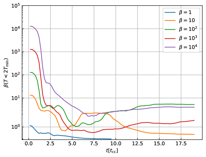
Figure 14: Evolution of plasma beta, $\beta$, for runs of ${t_{\rm cool,mix}/t_{\rm cc}}=0.1$ and $\beta=10^{4}$, $\beta=10^{3}$, $\beta=10^{2}$, $\beta=10$, $\beta=1$, represented by red, green, orange and blue solid lines, respectively. Curves kick off from their predetermined initial pressure to thermal ratio values and share a subsequent decrease. Final values are restricted well below 10, recovering values of beta $\beta\sim$ few for survived overdense clumps within the simulation box.

References

- Abruzzo et al. (2021) Abruzzo M. W., Bryan G. L., Fielding D. B., 2021, preprint
- Abruzzo et al. (2022) Abruzzo M. W., Fielding D. B., Bryan G. L., 2022, arXiv preprint arXiv:2210.15679
- Armillotta et al. (2017) Armillotta L., Fraternali F., Werk J. K., Prochaska J. X., Marinacci F., 2017, MNRAS, 470, 114
- Banda-Barragán et al. (2016) Banda-Barragán W., Parkin E., Federrath C., Crocker R., Bicknell G., 2016, MNRAS, 455, 1309
- Begelman & Fabian (1990) Begelman M. C., Fabian A., 1990, Monthly Notices of the Royal Astronomical Society, 244, 26P
- Bell et al. (2003) Bell E. F., Mcintosh D. H., Katz N., Weinberg M. D., 2003, ApJ, 585, 117
- Booth et al. (2012) Booth C. M., Schaye J., Delgado J. D., Dalla Vecchia C., 2012, MNRAS, 420, 1053
- Brook et al. (2011) Brook C., et al., 2011, Monthly Notices of the Royal Astronomical Society, 415, 1051
- Brüggen & Scannapieco (2016) Brüggen M., Scannapieco E., 2016, ApJ, 822, 31
- Brüggen et al. (2023) Brüggen M., Scannapieco E., Grete P., 2023, submitted to ApJ
- Bustard et al. (2016) Bustard C., Zweibel E. G., D’Onghia E., 2016, ApJ, 819, 29
- Butsky & Quinn (2018) Butsky I. S., Quinn T. R., 2018, The Astrophysical Journal, 868, 108
- Chandrasekhar (1961) Chandrasekhar S., 1961, Hydrodynamic and Hydromagnetic Stability. New York: Dover
- Chevalier & Clegg (1985) Chevalier R. A., Clegg A. W., 1985, Nature, 317, 44
- Chisholm et al. (2017) Chisholm J., Tremonti C. A., Leitherer C., Chen Y., 2017, Monthly Notices of the Royal Astronomical Society, 469, 4831
- Cottle et al. (2020) Cottle J., Scannapieco E., Brüggen M., Banda-Barragán W., Federrath C., 2020, ApJ, 892, 59
- Cowie & McKee (1977) Cowie L. L., McKee C. F., 1977, ApJ, 211, 135
- Cramer et al. (2019) Cramer W., Kenney J., Sun M., Crowl H., Yagi M., Jáchym P., Roediger E., Waldron W., 2019, The Astrophysical Journal, 870, 63
- Di Teodoro et al. (2018) Di Teodoro E. M., McClure-Griffiths N. M., Lockman F. J., Denbo S. R., Endsley R., Ford H. A., Harrington K., 2018, ApJ, 855, 33
- Dickey et al. (2013) Dickey J. M., et al., 2013, Publications of the Astronomical Society of Australia, 30
- Draine (2011) Draine B. T., 2011, Physics of the Interstellar and Intergalactic Medium. Princeton University Press
- Dursi & Pfrommer (2008) Dursi L. J., Pfrommer C., 2008, ApJ, 677, 993
- Dutta & Sharma (2019) Dutta A., Sharma P., 2019, arXiv preprint arXiv:1910.06339
- Farber & Gronke (2022) Farber R. J., Gronke M., 2022, Monthly Notices of the Royal Astronomical Society, 510, 551
- Farber et al. (2018) Farber R., Ruszkowski M., Yang H.-Y., Zweibel E. G., 2018, ApJ, 856, 112
- Farber et al. (2022) Farber R. J., Ruszkowski M., Tonnesen S., Holguin F., 2022, Monthly Notices of the Royal Astronomical Society, 512, 5927
- Faucher-Giguere & Oh (2023) Faucher-Giguere C.-A., Oh S. P., 2023, arXiv e-prints, p. arXiv:2301.10253
- Fielding & Bryan (2022) Fielding D. B., Bryan G. L., 2022, The Astrophysical Journal, 924, 82
- Fielding et al. (2018) Fielding D., Quataert E., Martizzi D., 2018, Monthly Notices of the Royal Astronomical Society, 481, 3325
- Fielding et al. (2020) Fielding D. B., Ostriker E. C., Bryan G. L., Jermyn A. S., 2020, ApJ, 894, L24
- Fox et al. (2019) Fox A. J., Richter P., Ashley T., Heckman T. M., Lehner N., Werk J. K., Bordoloi R., Peeples M. S., 2019, ApJ, 884, 53
- Fragile et al. (2005) Fragile P. C., Anninos P., Gustafson K., Murray S. D., 2005, The Astrophysical Journal, 619, 327
- Gatto et al. (2017) Gatto A., et al., 2017, Monthly Notices of the Royal Astronomical Society, 466, 1903
- Girichidis et al. (2016) Girichidis P., et al., 2016, Monthly Notices of the Royal Astronomical Society, 456, 3432
- Girichidis et al. (2021) Girichidis P., Naab T., Walch S., Berlok T., 2021, preprint
- Girichidis et al. (2022) Girichidis P., Pfrommer C., Pakmor R., Springel V., 2022, Monthly Notices of the Royal Astronomical Society, 510, 3917
- Gregori et al. (1999) Gregori G., Miniati F., Ryu D., Jones T., 1999, The Astrophysical Journal, 527, L113
- Gronke & Oh (2018) Gronke M., Oh S. P., 2018, MNRAS, 480, L111L115
- Gronke & Oh (2020) Gronke M., Oh S. P., 2020, MNRAS, 492, 1970
- Gronke et al. (2022) Gronke M., Oh S. P., Ji S., Norman C., 2022, Monthly Notices of the Royal Astronomical Society, 511, 859
- Grønnow et al. (2018) Grønnow A., Tepper-García T., Bland-Hawthorn J., 2018, ApJ, 865, 64
- Grønnow et al. (2022) Grønnow A., Tepper-García T., Bland-Hawthorn J., Fraternali F., 2022, Monthly Notices of the Royal Astronomical Society, 509, 5756
- Guo et al. (2010) Guo Q., White S., Li C., Boylan-Kolchin M., 2010, Monthly Notices of the Royal Astronomical Society, 404, 1111
- Gupta et al. (2021) Gupta A., Kingsbury J., Mathur S., Das S., Galeazzi M., Krongold Y., Nicastro F., 2021, The Astrophysical Journal, 909, 164
- Habegger et al. (2022) Habegger R., Zweibel E. G., Wong S., 2022, arXiv preprint arXiv:2211.04503
- Harris et al. (2020) Harris C. R., et al., 2020, Nature, 585, 357
- Heckman et al. (1990) Heckman T. M., Armus L., Miley G. K., 1990, Astrophysical Journal Supplement Series, 74, 833
- Hellsten et al. (1997) Hellsten U., Davé R., Hernquist L., Weinberg D. H., Katz N., 1997, The Astrophysical Journal, 487, 482
- Hillier & Arregui (2019) Hillier A., Arregui I., 2019, ApJ, 885, 101
- Holguin et al. (2019) Holguin F., Ruszkowski M., Lazarian A., Farber R., Yang H. K., 2019, Monthly Notices of the Royal Astronomical Society, 490, 1271
- Hopkins et al. (2021) Hopkins P. F., Chan T., Ji S., Hummels C. B., Kereš D., Quataert E., Faucher-Giguère C.-A., 2021, Monthly Notices of the Royal Astronomical Society, 501, 3640
- Hunter (2007) Hunter J. D., 2007, Computing In Science & Engineering, 9, 90
- Jacob et al. (2018) Jacob S., Pakmor R., Simpson C. M., Springel V., Pfrommer C., 2018, Monthly Notices of the Royal Astronomical Society, 475, 570
- Ji et al. (2018) Ji S., Oh S. P., McCourt M., 2018, MNRAS, 476, 852
- Jones et al. (1996) Jones T., Ryu D., Tregillis I., 1996, The Astrophysical Journal, 473, 365
- Jung et al. (2022) Jung S. L., Grønnow A., McClure-Griffiths N., 2022, arXiv e-prints, p. arXiv:2210.09722
- Kanjilal et al. (2021) Kanjilal V., Dutta A., Sharma P., 2021, MNRAS, 501, 1143
- Kim & Ostriker (2018) Kim C.-G., Ostriker E. C., 2018, The Astrophysical Journal, 853, 173
- Klein et al. (1994) Klein R. I., McKee C. F., Colella P., 1994, ApJ, 420, 213
- Lancaster et al. (2021) Lancaster L., Ostriker E. C., Kim J.-G., Kim C.-G., 2021, The Astrophysical Journal, 914, 89
- Larson (1974) Larson R. B., 1974, Monthly Notices of the Royal Astronomical Society, 169, 229
- Lequeux et al. (1979) Lequeux J., Peimbert M., Rayo J., Serrano A., Torres-Peimbert S., 1979, Astronomy and Astrophysics, 80, 155
- Li & Bryan (2020) Li M., Bryan G. L., 2020, The Astrophysical Journal Letters, 890, L30
- Li et al. (2020) Li Z., Hopkins P. F., Squire J., Hummels C., 2020, MNRAS, 492, 1841
- Lita et al. (2021) Lita M., Schneider E. E., Ostriker E. C., 2021, The Astrophysical Journal, 919, 112
- Lochhaas et al. (2021) Lochhaas C., Thompson T. A., Schneider E. E., 2021, Monthly Notices of the Royal Astronomical Society, 504, 3412
- Mac Low & Ferrara (1999) Mac Low M.-M., Ferrara A., 1999, ApJ, 513, 142
- Mac Low et al. (1994) Mac Low M.-M., McKee C. F., Klein R. I., Stone J. M., Norman M. L., 1994, ApJ, 433, 757
- Mandelker et al. (2020) Mandelker N., Nagai D., Aung H., Dekel A., Birnboim Y., van den Bosch F. C., 2020, Monthly Notices of the Royal Astronomical Society, 494, 2641
- Marinacci et al. (2010) Marinacci F., Binney J., Fraternali F., Nipoti C., Ciotti L., Londrillo P., 2010, MNRAS, 404, 1464
- Martizzi et al. (2016) Martizzi D., Fielding D., Faucher-Giguère C.-A., Quataert E., 2016, Monthly Notices of the Royal Astronomical Society, 459, 2311
- McCourt et al. (2015) McCourt M., O’Leary R. M., Madigan A.-M., Quataert E., 2015, MNRAS, 449, 2
- McCourt et al. (2018) McCourt M., Oh S. P., O’Leary R., Madigan A.-M., 2018, MNRAS, 473, 5407
- Moss & Sokoloff (2017) Moss D., Sokoloff D., 2017, Astronomy & Astrophysics, 598, A72
- Murthy et al. (2021) Murthy S., Morganti R., Oosterloo T., Maccagni F. M., 2021, Astronomy & Astrophysics, 654, A94
- Naab & Ostriker (2017) Naab T., Ostriker J. P., 2017, Annual review of astronomy and astrophysics, 55, 59
- Nittmann et al. (1982) Nittmann J., Falle S., Gaskell P., 1982, Monthly Notices of the Royal Astronomical Society, 201, 833
- Pakmor et al. (2016) Pakmor R., Pfrommer C., Simpson C. M., Springel V., 2016, The Astrophysical Journal Letters, 824, L30
- Pandya et al. (2020) Pandya V., et al., 2020, The Astrophysical Journal, 905, 4
- Pandya et al. (2021) Pandya V., et al., 2021, Monthly Notices of the Royal Astronomical Society, 508, 2979
- Pfrommer & Dursi (2010) Pfrommer C., Dursi J., 2010, Nature Physics, 6, 520
- Poggianti et al. (2017) Poggianti B. M., et al., 2017, ApJ, 844, 48
- Pourtsidou (2017) Pourtsidou A., 2017, arXiv preprint arXiv:1709.07316
- Putman et al. (2002) Putman M. E., et al., 2002, The Astronomical Journal, 123, 873
- Qu et al. (2022) Qu Z., et al., 2022, Monthly Notices of the Royal Astronomical Society, 516, 4882
- Rathjen et al. (2021) Rathjen T.-E., et al., 2021, Monthly Notices of the Royal Astronomical Society, 504, 1039
- Rathjen et al. (2022) Rathjen T.-E., Naab T., Walch S., Seifried D., Girichidis P., Wünsch R., 2022, arXiv preprint arXiv:2211.15419
- Robertson et al. (2010) Robertson B. E., Kravtsov A. V., Gnedin N. Y., Abel T., Rudd D. H., 2010, MNRAS, 401, 2463
- Rudie et al. (2019) Rudie G. C., Steidel C. C., Pettini M., Trainor R. F., Strom A. L., Hummels C. B., Reddy N. A., Shapley A. E., 2019, The Astrophysical Journal, 885, 61
- Rupke (2018) Rupke D., 2018, Galaxies, 6, 138
- Ruszkowski et al. (2014) Ruszkowski M., Brüggen M., Lee D., Shin M.-S., 2014, The Astrophysical Journal, 784, 75
- Ruszkowski et al. (2017) Ruszkowski M., Yang H.-Y. K., Zweibel E., 2017, The Astrophysical Journal, 834, 208
- Ryu et al. (2000) Ryu D., Jones T., Frank A., 2000, The Astrophysical Journal, 545, 475
- Scannapieco & Brüggen (2015) Scannapieco E., Brüggen M., 2015, ApJ, 805, 158
- Schneider & Robertson (2018) Schneider E. E., Robertson B. E., 2018, The Astrophysical Journal, 860, 135
- Shin et al. (2008) Shin M.-S., Stone J. M., Snyder G. F., 2008, The Astrophysical Journal, 680, 336
- Simpson et al. (2016) Simpson C. M., Pakmor R., Marinacci F., Pfrommer C., Springel V., Glover S. C., Clark P. C., Smith R. J., 2016, The Astrophysical Journal Letters, 827, L29
- Somerville & Davé (2015) Somerville R. S., Davé R., 2015, ARA&A, 53, 51
- Sparre et al. (2019) Sparre M., Pfrommer C., Vogelsberger M., 2019, MNRAS, 482
- Sparre et al. (2020) Sparre M., Pfrommer C., Ehlert K., 2020, MNRAS, 499, 4261
- Stacey et al. (2022) Stacey H., Costa T., McKean J., Sharon C., Calistro Rivera G., Glikman E., van der Werf P., 2022, Monthly Notices of the Royal Astronomical Society, 517, 3377
- Steidel et al. (2010) Steidel C. C., Erb D. K., Shapley A. E., Pettini M., Reddy N., Bogosavljevi M., Rudie G. C., Rakic O., 2010, ApJ, 717, 289
- Steinwandel et al. (2022a) Steinwandel U. P., Kim C.-G., Bryan G. L., Ostriker E. C., Somerville R. S., Fielding D. B., 2022a, arXiv preprint arXiv:2212.03898
- Steinwandel et al. (2022b) Steinwandel U. P., Dolag K., Lesch H., Burkert A., 2022b, The Astrophysical Journal, 924, 26
- Stone & Gardiner (2007a) Stone J. M., Gardiner T., 2007a, Physics of Fluids, 19, 094104
- Stone & Gardiner (2007b) Stone J. M., Gardiner T., 2007b, The Astrophysical Journal, 671, 1726
- Stone & Norman (1992) Stone J. M., Norman M. L., 1992, ApJ, 173, 17
- Stone et al. (2008) Stone J. M., Gardiner T. A., Teuben P., Hawley J. F., Simon J. B., 2008, The Astrophysical Journal Supplement Series, 178, 137
- Strickland & Heckman (2009) Strickland D. K., Heckman T. M., 2009, ApJ, 697, 2030
- Su et al. (2021) Su Y., et al., 2021, ApJ, 910, 131
- Sutherland & Dopita (1993) Sutherland R. S., Dopita M. A., 1993, ApJS, 88, 253
- Tan et al. (2021) Tan B., Oh S. P., Gronke M., 2021, MNRAS, 502, 3179
- Tan et al. (2022) Tan B., Oh S. P., Gronke M., 2022, arXiv preprint arXiv:2210.06493
- Thompson et al. (2016) Thompson T. A., Quataert E., Zhang D., Weinberg D. H., 2016, Monthly Notices of the Royal Astronomical Society, 455, 1830
- Tonnesen & Bryan (2010) Tonnesen S., Bryan G. L., 2010, ApJ, 709, 1203
- Tonnesen & Bryan (2012) Tonnesen S., Bryan G. L., 2012, MNRAS, 422, 1609
- Tonnesen & Bryan (2021) Tonnesen S., Bryan G. L., 2021, The Astrophysical Journal, 911, 68
- Tonnesen & Stone (2014) Tonnesen S., Stone J., 2014, The Astrophysical Journal, 795, 148
- Townsend (2009) Townsend R., 2009, ApJS, 181, 391
- Tremonti et al. (2004) Tremonti C. A., et al., 2004, The Astrophysical Journal, 613, 898
- Tumlinson et al. (2005) Tumlinson J., Shull J. M., Giroux M. L., Stocke J. T., 2005, The Astrophysical Journal, 620, 95
- Tumlinson et al. (2017) Tumlinson J., Peeples M. S., Werk J. K., 2017, arXiv preprint arXiv:1709.09180
- Turk et al. (2010) Turk M. J., Smith B. D., Oishi J. S., Skory S., Skillman S. W., Abel T., Norman M. L., 2010, ApJS, 192, 9
- Übler et al. (2014) Übler H., Naab T., Oser L., Aumer M., Sales L. V., White S. D., 2014, Monthly Notices of the Royal Astronomical Society, 443, 2092
- Veilleux et al. (2005) Veilleux S., Cecil G., Bland-Hawthorn J., 2005, Annu. Rev. Astron. Astrophys., 43, 769
- Veilleux et al. (2020) Veilleux S., Maiolino R., Bolatto A. D., Aalto S., 2020, The Astronomy and Astrophysics Review, 28, 1
- Waagan et al. (2011) Waagan K., Federrath C., Klingenberg C., 2011, Journal of Computational Physics, 230, 3331
- Weaver et al. (1977) Weaver R., McCray R., Castor J., Shapiro P., Moore R., 1977, The Astrophysical Journal, 218, 377
- Werk et al. (2014) Werk J. K., et al., 2014, The Astrophysical Journal, 792, 8
- Wheatley et al. (2005) Wheatley V., Pullin D. I., Samtaney R., 2005, J. Fluid Mech, 552, 179
- Wiersma et al. (2009) Wiersma R. P., Schaye J., Smith B. D., 2009, Monthly Notices of the Royal Astronomical Society, 393, 99
- Xu & Stone (1995) Xu J., Stone J. M., 1995, ApJ, 454, 172
- Xu et al. (2022) Xu X., et al., 2022, ApJ, 933, 222
- Zhang (2018) Zhang D., 2018, Galaxies, 6, 114
- Zhang et al. (2017) Zhang D., Thompson T. A., Quataert E., Murray N., 2017, Monthly Notices of the Royal Astronomical Society, 468, 4801