On a generalised Lambert branch transition function arising from -binomial coefficients
Abstract.
With only a complete solution in dimension one and partially solved in dimension two, the Lenz-Ising model of magnetism is one of the most studied models in theoretical physics. An approach to solving this model in the high-dimensional case () is by modelling the magnetisation distribution with -binomial coefficients. The connection between the parameters and the distribution peaks is obtained with a transition function which generalises the mapping of Lambert function branches and to each other. We give explicit formulas for the branches for special cases. Furthermore, we find derivatives, integrals, parametrizations, series expansions, and asymptotic behaviors.
Key words and phrases:
Generalization of Lambert W function, Lenz-Ising model, magnetization distribution, -binomial coefficients, special functions2020 Mathematics Subject Classification:
Primary 33B99, 33F05, 82B20; Secondary 05A10, 05A301. Introduction and background
We will study the transition function that arises when using -binomial coefficients to attack the model of magnetism in statistical mechanics for higher dimensions. To get an overall view of our study, we start in Section 1.1 with a physical background on the Lenz-Ising model. In Section 1.2 we give an introduction to -binomial coefficients, and how it relates to the given physical problem. Section 1.2 will also reveal how the transition function arises and it’s relation to the Lambert function.
1.1. Physical origins
The Lenz-Ising model, usually referred to as the Ising model, was introduced by Wilhelm Lenz [16] in 1920 as a simple model for magnetism. The time was ripe for such a model after the discoveries by Pierre Curie111In his thesis 1895. He and his wife Marie later shared the 1903 Nobel prize in physics with Becquerel for their work on radioactivity. that magnetic materials (iron, cobalt, nickel, etc.) undergo a phase transition at a critical temperature , the Curie temperature, above which they lose their permanent magnetic properties. In the Ising model without an external field, the material is described as a system of interacting particles, each having spin , and is governed by the temperature [7, 11, 20]. The system in question can be any finite graph, with the vertices corresponding to the particles and the edges indicating which particles interact. In the model’s most famous version, the system is the (infinite) -dimensional integer lattice. The -dimensional model (an infinite chain of particles) was solved in 1925 by Lenz’s student, Ernst Ising, in his thesis [14]. Unfortunately, the result was disappointing since he showed that this system does not have a phase transition at any positive temperature, the critical temperature being .
It took until 1944 when the Norwegian chemist Lars Onsager222Nobel prize in chemistry 1968 for his work on the thermodynamics of irreversible processes. solved the model for 2-dimensional systems [21]. This solution was considered a major breakthrough, rendering a positive critical temperature, (assuming unit interaction between nearest-neighbor particles in the lattice). Unfortunately, again, the techniques used by Onsager did not point to a solution for the 3-dimensional model. In fact, to this day, very little is known rigorously about the 3-dimensional model, and the 2-dimensional model with an external field is still unsolved. For dimensions the critical exponents, which govern the behaviour of various quantities near the critical point, are known exactly but the critical temperature is still not known exactly for any .
This has not made the Ising model any less attractive, instead, it has generated a staggering number of papers studying many variants of the model in different dimensions [23, 5, 22, 12]. Also it has become a testing bed for various Monte Carlo simulation algorithms [26, 25, 13].
Let us focus a little closer on an interesting aspect of the Ising model without an external field, namely its magnetization distribution. The magnetization of the Ising model is the sum of all the spins in the system, , so that for a system with spins we have . For a finite -dimensional system (we assume ), at any given temperature , the magnetization obeys a symmetric distribution with peaks at , for some . Now, for temperatures above the Curie temperature (), the distribution of magnetizations is unimodal with its peak at so that . When we lower the temperature below the Curie temperature () the distribution becomes bimodal with peaks at for , with as . The parameter here corresponds to the so-called spontaneous magnetization of the Ising model, but its relation to is only known exactly for -dimensional (infinite) systems. It was conjectured by Onsager in 1948 and proved by Yang in 1952 (see [19] for details) that in this case
where . Thus a phase transition occurs at when becomes positive. In physical terms, the unimodal distribution corresponds to losing the magnetic properties, whereas the bimodal distribution corresponds to retaining them. Finding a corresponding formula for dimensions would be a major breakthrough.
1.2. The -binomial coefficients
It was suggested in [17] that the magnetization distribution is well described by -binomial coefficients for finite high-dimensional systems (). In fact, in a special case (mean-field), they are equivalent, and for they have the same asymptotic shape when . In principle, one could then model the magnetization distribution for a finite system at temperature with a -binomial distribution where and depend on according to some functions and . It would be a more realistic project to find these functions for temperatures very close to and one such attempt was made in [18].
However, it should be mentioned that the -binomial coefficients have received attention also for other interesting purely mathematical properties [2, 3, 9].
Let us here provide some more detail on these coefficients. The -binomial coefficient [8] is defined for as
from which a symmetric -binomial distribution [17, 18] is defined to have a probability mass function proportional to the sequence of these coefficients. Note that the sum of the -binomial coefficients do not seem to have a simple expression, as opposed to standard binomial coefficients for which the sum is simply . For it has been shown [24] that the coefficients either form a unimodal sequence with maximum at , or, a bimodal sequence with maxima at and for some . We let the parameter control the location of the sequence maximum by defining
Having two consecutive -binomial coefficients, indexed and , being equal leads, after simplification, to the equation
| (1.1) |
We here need to introduce the -parameterizations
though other parameterizations are also of interest. With and fixed we now solve for .
1.3. Introducing the functions and
First the special case . The asymptotic form of the ratio in (1.1) now becomes simply
and to receive a leading term of we must have . This defines a special case of the transition function :
| (1.2) |
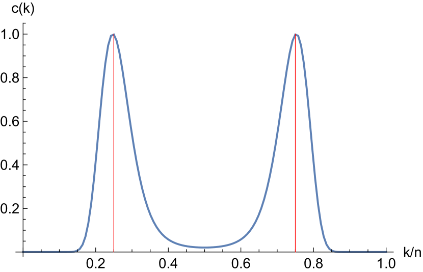
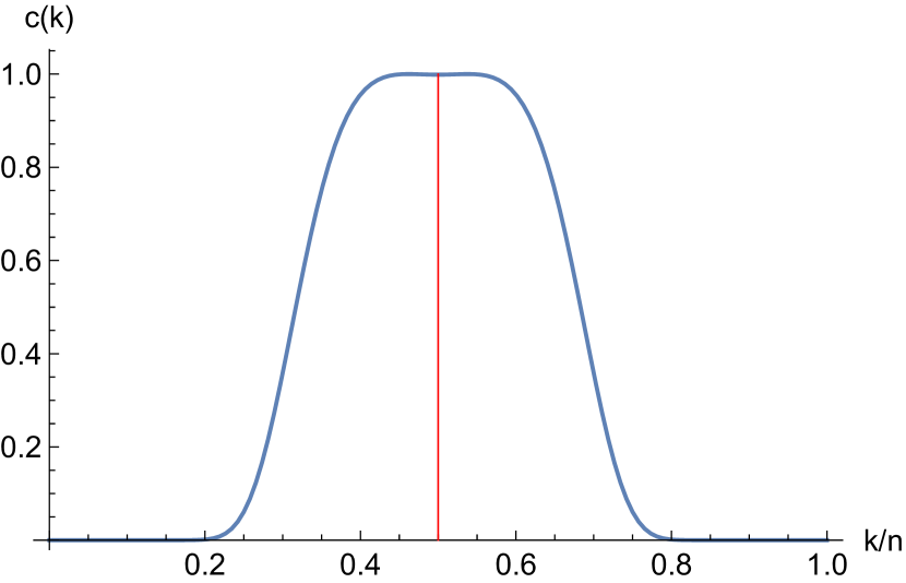
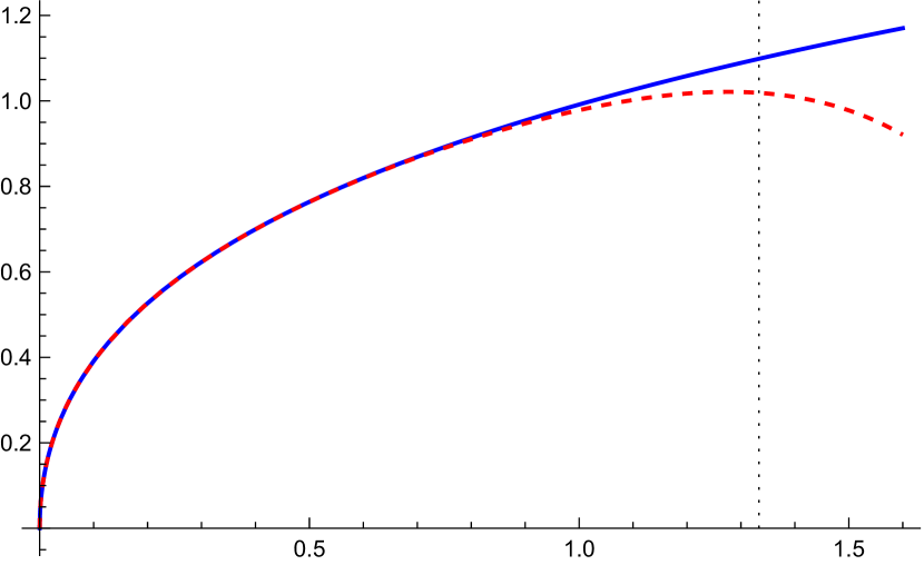
Here denotes the famous Lambert function, which returns one of two real solutions of the equation . The principal solution, defined for , gives and the other branch, defined for , gives . The transition function thus maps solutions between the two branches of the Lambert function. The coefficient sequence then will have its two maxima at points where . In Fig. 1 the right panel shows an example of this case and the left panel shows the case .
We will now generalise the transition function of to the case of . The ratio of (1.1) now becomes
so to receive the correct leading term of we must now solve
| (1.3) |
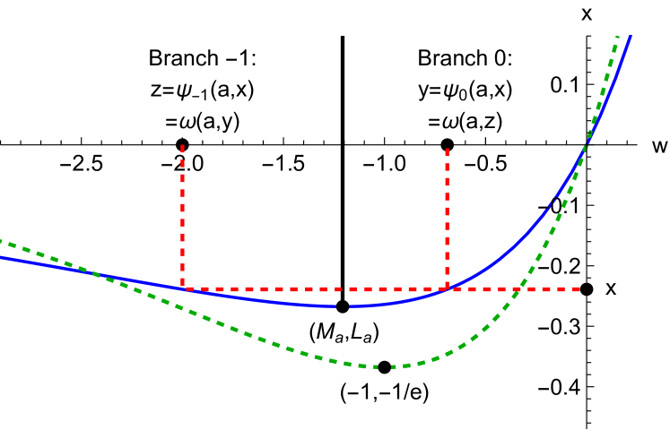
We therefore define the function
and introduce its inverse function as one of the two real solutions of
We note that takes its minimum value at , where
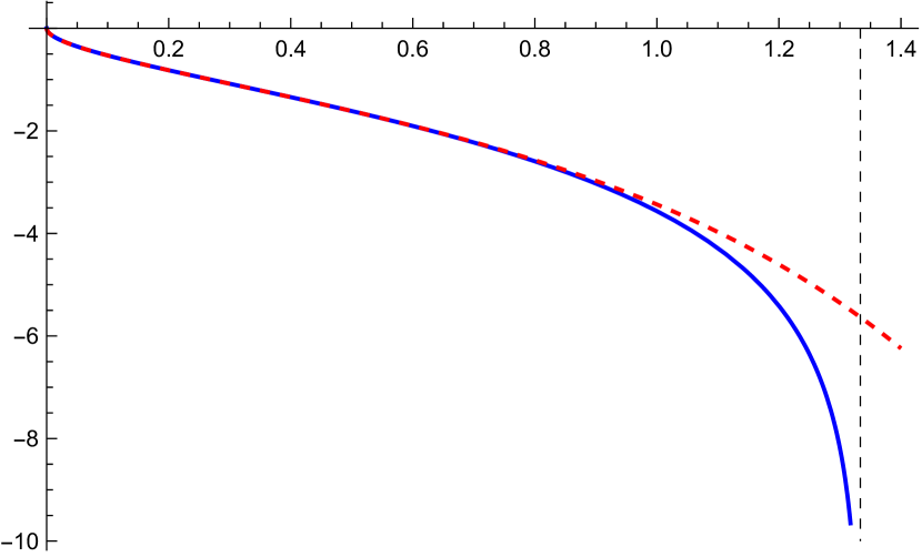
The principal branch is now defined for , while the other branch is defined for . Thus is the branch separator with and . In Fig. 2 we show how the equation relates to the definition and .
The transition function , defined above only for in (1.2), can now be generalized to
| (1.4) |
Plots of and are shown in Fig. 3.
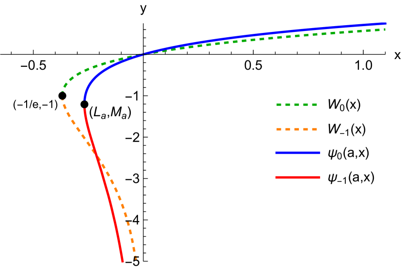
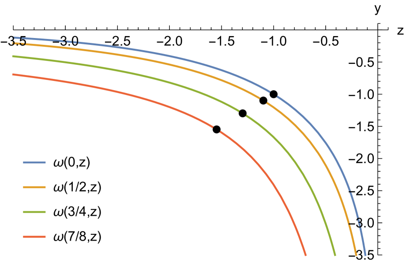
Note that so that for is indeed a natural and continuous generalisation of the transition function for Lambert of (1.2). However, the function is only related to the Lambert for small . In that case we have so that
for both branches, where the functions are defined. Let us also briefly state the following properties of .
-
(1)
is a fixed point, i.e., .
-
(2)
is an involution, i.e., for all .
-
(3)
is negative, decreasing and concave for all .
-
(4)
and .
The transition function was used in [17], though in a slightly different guise, and very little was mentioned with regard to its mathematical properties. This article aims to remedy this by first investigating the properties of and apply this to .
To conclude this section, the -binomial coefficient sequence will then have its peaks at where and the parameter controls the mass shape of the sequence, see Fig. 1. Note that the peaks are never at exactly . To obtain this the resulting would also depend on and a special function is needed. We would then have when .
2. Results on the - and -functions from elementary techniques
In this section we will show some basic properties of the and -function obtained only from elementary techniques. Also we solve some interesting special cases. Later in the article we will use more powerful methods and extend these results considerably.
2.1. The boundary cases and and a lower bound for
First we recall that
| (2.1) |
The limits for and when is fixed are then
For fixed we also have:
-
(1)
If is positive then is increasing for .
-
(2)
If is negative then is decreasing for .
Now we can define the limit forms of . Solving for in gives the limit inverse function
thanks to uniform convergence. In fact, since is increasing with respect to then is decreasing with so that we receive the inequality
In Theorem 8.1 below we will give a much sharper bound, but requiring considerably more work. Since is strictly increasing for all , thus having no second branch, we obtain no limit . Also, since we have no well-defined inverse function .
2.2. A parametrization of for general
In Section 4 we will use a powerful technique which gives a parametrization of both branches and for . However, here we only require an elementary technique which allows us to develop a parametrization of for . First we define
Then , and therefore . Hence, so that . Finally, we now require , thus giving the branch , so that we can obtain
which gives the sought-after parametrization, defined for :
2.3. Special values of and for general
The -branch is more difficult to parametrize for general . However, it is easy to give an infinite sequence of points satisfying and we will do so here.
Note that it is an easy exercise to show that the th derivative of vanishes at th multiples of , so that
| (2.2) |
If we define
| (2.3) |
so that and is the inflection point of etc, then
| (2.4) |
Of course, since for , this only gives the solutions in branch of the equation , thus leading to
| (2.5) |
Since there is also a corresponding solution for but this value does not seem to have a simple expression. However, for special values of we can find closed form expressions for but we will return to this in Section 4.
2.4. The special case : explicit formulas of and
In general it is difficult to find explicit formulas for and . However, for some special cases of we will be successful and the case turns out to be surprisingly easy to handle. In Section 4 we will give formulas for and at other rational values of but they are considerably more complicated since they are based on the roots of the quartic polynomials. The formulas given here for and seem to be the only simple exact solutions.
To compute we need to solve for in the equation . When we then receive
| (2.6) |
where
Solving the second degree polynomial gives the roots
| (2.7) |
where the two solutions correspond to the two branches so that
| (2.8) | ||||
| (2.9) |
We now combine this with the definition of in (1.4). The case corresponds to and we receive
The other case gives so that
We thus receive the same formula in both cases so we conclude that
| (2.10) |
2.5. is transcendental number
We shall prove that if is algebraic number (), then is transcendental number (). To prove it we need Lindemann-Weierstrass Theorem ( [4, Theorem 1.4]), i.e., if and are distinct numbers, then the equation
has only the trivial solution .
Proposition 2.1.
If , , then .
Proof.
Assume that , and . Then and therefore . By the definition of we have
which is impossible by the Lindemann-Weierstrass Theorem. ∎
3. Derivatives and a primitive function of
In Proposition 3.1, we provide a formula for the th derivative of with respect to . Here, a shorter notation , is used referring to both branches, and is treated as a fixed parameter. A primitive function of is obtained later in Proposition 3.2.
Proposition 3.1.
For
| (3.1) |
where the polynomials are given by the following recurrence formula: and
Proof.
We proceed by induction. We shall use the shorter notation when referring to both branches. The case , can be deduced by using the implicit function theorem:
with the special value
Assume next that (3.1) is valid for some natural number . Let us define
We then have
and we can conclude the desired result by the induction axiom. ∎
Example 3.2.
Proposition 3.3.
The function
| (3.2) |
is a primitive function of .
Proof.
Using the substitution , , we get
∎
Remark.
In a similar manner, using the substitution , one can prove that integrals of the form
can be integrated in an elementary way.
Exploiting the Taylor series , and the value , we have
Hence, we can now compute the following definite integral:
and, since is the inverse of ,
4. Explicit formulas for
In this section we shall, for certain rational values of , find explicit formulas for both branches of the -function and the transition function . We let denote the real-valued positive solution(s) to the polynomial equation . Recall that
| (4.1) |
For natural numbers and such that we set
so that
Using the substitution we rewrite (4.1) as
and then
| (4.2) |
We are then able to give explicit solutions to this equation from classical methods in the following cases:
And the case has already been treated in Section 2.
Case a=1/2: After some straightforward but rather lengthy calculations using Cardano’s method for solving cubic equations, we arrive at the following:
and
which then gives the transition function
Case a=1/5: Again using Cardano’s method for solving cubic equations, we get in this case:
and
And now we obtain the transition function
In the following cases we will only state the -functions.
Case a=3/5: In this case we shall solve
by using Ferrari’s method. First we need the solution to the auxiliary equation:
In our case, , so that
and we then arrive at
Furthermore,
Case a=1/7: In this case we shall solve
by using Ferrari’s method. After some lengthy but straightforward calculations we get:
and
where
5. A parametrization and a definite integral
The main aim of this section is to prove that
We rely on an ingenious idea to simultaneously parameterize both branches of for . This idea originates from [10], and is explained in [15, Theorem 1.3.1]. Our parametrization is presented in the following theorem:
Theorem 5.1.
Let
where . Then
Proof.
We are looking for such that
Let , where is a parameter. Then,
which implies
Hence,
Continuing in a similar manner, we set , where is a parameter, which implies
Hence,
which yields
Thus, for it holds
Set where . Then
∎
Thanks to the parametrization in Theorem 5.1 we get an alternative way to find explicit formulas for , and . The below example is for the case .
Example 5.2.
Employing Theorem 5.1, we can now state the following theorem:
Theorem 5.3.
Proof.
The definition of the transition function states:
For in the relation we note that one inverse branch is , and the other branch is . Hence,
From Theorem 5.1 it follows
and therefore
where
Finally, from the substitution it follows
∎
6. Taylor series of at zero
In this section and the next, we will focus on series expansions. Here we use Lagrange’s inversion theorem to determine the Taylor series for about (see (6.1)). First let us recall Lagrange’s inversion theorem [1, 6]:
Theorem 6.1 (Lagrange’s inversion theorem).
If , , for some real-analytic function in a neighbourhood of with , then
where the convergence radius is strictly positive. Furthermore, if
then it holds
where , is the rising factorial and is the partial exponential Bell polynomial.
We apply this theorem to the function
and then we arrive at
where
Thus, the first few terms of the Taylor series of around are given by:
| (6.1) |
Furthermore, the radius of converges of the Taylor series can not exceed .
7. Series expansions of at and of at
This section aims to determine the series expansions of at and of at with the help of Proposition 7.1 as a tool. The series are stated in (7.1), (7.2), and (7.3), respectively.
Proposition 7.1.
Let be a smooth function in the neighborhood of such that and . Then has two smooth inverse functions (in some neighborhood of ), a right inverse for , and a left inverse for , which can be expressed as
where and for .
Proof.
Without loss of generality, we may assume that is convex in a possible smaller neighborhood of zero. The Taylor expansion at zero can be presented as
Therefore, for some smooth function with . Thus, is smooth in the neighborhood of . Set
The function is invertible and smooth in a possible punctured neighborhood of . Furthermore, for all the following limits exist:
and . From this it follows that has two smooth inverse functions, , which can be expressed as and , . Finally, by applying the Taylor series expansion to we get the desired conclusion. ∎
Let and recall that . Then we receive the following series expansion around
The inverse series expansion gives us can be found by using the series ansatz of and in Proposition 7.1 and solve term by term.
| (7.1) |
which converges for . Note that the coefficients of and can change sign for .
Thanks to Proposition 7.1 we can deduce the other branch
| (7.2) |
and again this series converges for . Note that the second argument in both series is .
Now we find the composition of the series of with that of , which gives us the series of , and note that the -factor cancels out,
| (7.3) |
Note that the coefficient of is the first which depends on .
Note also that the coefficient of is the first which can become
zero for some . This happens at . The coefficient
for becomes zero at .
Example 7.2.
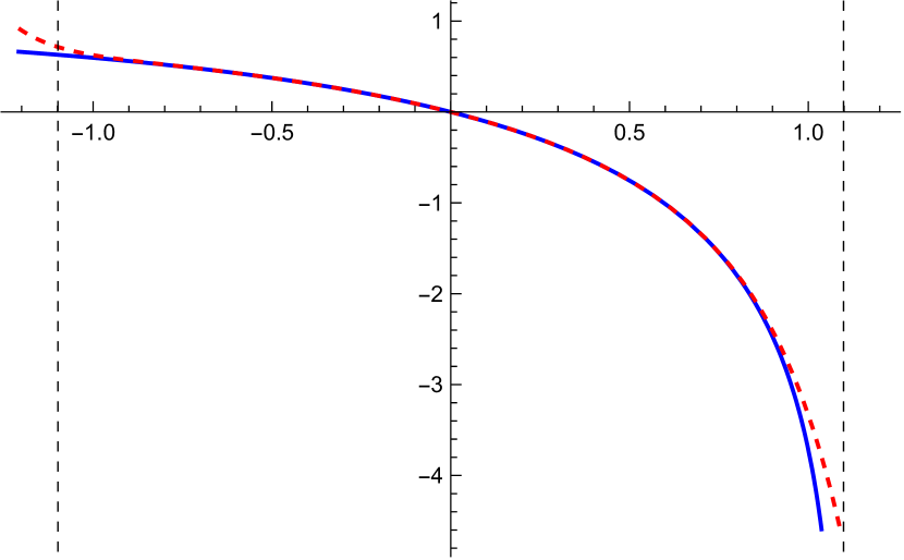
In Fig. 4 we show , , for and their respective series expansion as just stated. In this case the first few terms of the respective expansions are
8. Asymptotics of the branch as
Here we determine the asymptotic behaviour of as . An important tool in doing so is the following theorem.
Theorem 8.1.
Let
Then the following holds
-
(1)
if , then
-
(2)
if , then
Remark.
Let be the point such that the bounds hold when . Numerical experimentation suggests that for the lower bounds we have
-
If then
This seems to be the exact optimal point when . It is not optimal when but it still works then.
-
If then works. The difference between and the lower bound is decreasing when (this is the limit when ).
For the upper bounds we get
-
If then . The difference between the upper bound and is decreasing for . Both of these formulas are rough estimates but they are much smaller than the -bound in the theorem. In any case, the upper bounds require very large if they are to hold for small .
-
When the upper bound holds for all .
-
When the difference between the upper bound and is decreasing for all .
Let us start with observing that if , then
and therefore we get
We shall next continue with proving two auxiliary lemmas.
Lemma 8.2.
For it holds
for all . In particular,
Proof.
Using the definition of and the fact that function is increasing we have
The last term above tends to as , which proves the final claim. ∎
The following lemma is a straight-forward exercise obtained from taking the Taylor expansion of about .
Lemma 8.3.
For any there exists a point such that
-
, and
-
,
for all . Furthermore, for there exists a point such that
for all . In fact in both cases one can take .
We are now ready to present the proof of the main result of this section.
Proof of Theorem 8.1..
From Lemma 8.2 it follows that satisfies: , , as and , where
Next, substitute in the implicit definition of , and we arrive at
and after a rearrangement we obtain
| (8.1) |
As a corollary of the previous proof, we can get a series expansion in the variable . First we re-state (8.1):
and then we use the Taylor expansion of the exponential function about :
where , , , . Then by using Theorem 6.1 we arrive at
where
and , is the rising factorial and denote the partial or incomplete exponential Bell polynomials.
Let us compute a few coefficients:
Thus,
which implies
9. Asymptotics of the branch as
Using the same techniques as in the previous sections, we shall study the branch ’s behavior near zero. We shall prove the following theorem. Recall that the branch is defined for .
Theorem 9.1.
Let . Then
-
(1)
-
(2)
-
(3)
For it holds
In the proof of Theorem 9.1 we shall need the following elementary facts.
Lemma 9.2.
For it holds
-
and
-
.
Proof of Theorem 9.1..
(1) If , then
| (9.1) |
and therefore we get
| (9.2) |
Then, let . We know that . From (9.1) it follows
and after rearranging we have
| (9.3) |
Each term of the left side is bounded and since the right hand side tends to zero, when , then so does .
(2) Using the definition of , and the fact that the function is increasing and by (9.2) we have
Proceeding in a similar manner as in Section 8, we get an expansion of in terms of :
References
- [1] Abramowitz, M., and Stegun, I. A. Handbook of mathematical functions with formulas, graphs and mathematical tables. Dover, New York, 1972.
- [2] Ahmia, M., and Belbachir, H. -analogue of a linear transformation preserving log-convexity. Indian J. Pure Appl. Math. 49, 3 (2018), 549–557.
- [3] Ahmia, M., and Belbachir, H. Preserving log-concavity for -binomial coefficients. Discrete Math. Algorithms Appl. 11, 2 (2019), 1950017.
- [4] Baker, A. Transcendental number theory. Cambridge University Press, Cambridge, 1975.
- [5] Baxter, R. J. Potts model at the critical temperature. J. Phys. C: Solid State Phys. 6, 23 (1973), L445.
- [6] Charalambides, C. A. Enumerative combinatorics. Chapman&Hall/CRC, Boca Raton, Florida, 2002.
- [7] Cipra, B. A. An introduction to the Ising model. Amer. Math. Monthly 94 (1987), 937–959.
- [8] Corcino, R. B. On -binomial coefficients. INTEGERS: Electronic journal of combinatorial number theory 8 (2008), #A29.
- [9] Corcino, R. B., Gonzales, K. J. M., Loquias, M. J. C., and Tan, E. L. Dually weighted Stirling-type sequences. Eur. J. Combin. 43 (2015), 55–67.
- [10] Corless, R. M., Gonnet, G. H., Hare, D. E. G., Jeffrey, D. J., and Knuth, D. E. On the Lambert function. Adv. Comput. Math. 5, 4 (1996), 329–359.
- [11] Duminil-Copin, H. 100 years of the (critical) Ising model on the hypercubic lattice. https://arxiv.org/abs/2208.00864, 2022. To appear in Proceedings of the ICM 2022.
- [12] Edwards, S. F., and Anderson, P. W. Theory of spin glasses. J. Phys. F: Met. Phys. 5 (1975), 965–974.
- [13] Ferrenberg, A. M., Xu, J., and Landau, D. P. Pushing the limits of Monte Carlo simulations for the three-dimensional Ising model. Phys. Rev. E 97 (2018), 043301.
- [14] Ising, E. Beitrag zur Theorie des Ferromagnetismus. Z. Physik 31 (1925), 253–258.
- [15] Kalugin, A. Analytical properties of the Lambert W function. PhD thesis, The University of Western Ontario, London, Ontario, Canada, 2011.
- [16] Lenz, W. Beitrag zum Verständnis der magnetischen Erscheinungen in festen Körpern. Physik. Z. 21 (1920), 613–615.
- [17] Lundow, P. H., and Rosengren, A. On the -binomial distribution and the Ising model. Phil. Mag. 90, 24 (2010), 3313–3353.
- [18] Lundow, P. H., and Rosengren, A. The -binomial distribution applied to the 5d Ising model. Phil. Mag. 93, 14 (2013), 1755–1770.
- [19] McCoy, B. M., and Wu, T. T. The two-dimensional Ising model. Harvard University Press, 1973.
- [20] Okounkov, A. The Ising model in our dimension and our times. https://arxiv.org/abs/2207.03874, 2022. To appear in Proceedings of the ICM 2022.
- [21] Onsager, L. Crystal statistics I. A two-dimensional model with an order-disorder transition. Phys. Rev. (2) 65 (1944), 117–149.
- [22] Sherrington, D., and Kirkpatrick, S. Solvable model of a spin-glass. Phys. Rev. Lett. 35, 26 (1975), 1792–1796.
- [23] Stanley, H. E. Dependence of critical properties of dimensionality of spins. Phys. Rev. Lett. 20, 12 (1968), 589–592.
- [24] Su, X.-T., and Wang, Y. Proof of a conjecture of Lundow and Rosengren on the bimodality of -binomial coefficients. J. Math. Anal. Appl. 391, 2 (2012), 653 – 656.
- [25] Wang, F., and Landau, D. P. Efficient, multiple-range random walk algorithm to calculate the density of states. Phys. Rev. Lett 86, 10 (2001), 2050–2053.
- [26] Wolff, U. Collective Monte Carlo for updating for spin systems. Phys. Rev. Lett. 62, 4 (2001), 361–364.