Transvese momentum dependent parton distributions of pion at leading twist

Abstract

We calculate the leading twist pion unpolarized transverse momentum distribution $f_{1}(x,k_{T}^{2})$ and the Boer-Mulders function $h_{1}^{\perp}(x,k_{T}^{2})$, using leading Fock-state light front wave functions (LF-LFWFs) based on Dyson-Schwinger and Bethe-Salpeter equations. These DS-BSEs based LF-LFWFs provide dynamically generated s- and p-wave components, which are indispensable in producing chirally odd Boer-Mulders function that has one parton spin flipped. Employing a non-perturbative SU(3) gluon rescattering kernel to treat the gauge link of the Boer-Mulders function, we thus obtain both TMDs at hadronic scale and then evolve them to the scale of $\mu^{2}=4.0$ GeV². We finally calculate the generalized Boer-Mulders shift and find it to be in agreement with the lattice prediction.

I Introduction

Multidimensional imaging of hadrons has excited a lot of interest for the last several decades. Transverse momentum dependent parton distributions functions (TMDs) contain important information of the three-dimensional internal structure of hadrons, especially the spin-orbit correlations of quarks within them Sivers (1990); Boer and Mulders (1998); Barone et al. (2002); Collins (2003); Angeles-Martinez et al. (2015). The TMDs of the pion and nucleon, which are spin-$0$ and spin-$1/2$ respectively, have thus received extensive studies from phenomenological models Pasquini et al. (2005, 2008); Bacchetta et al. (2008); Pasquini and Schweitzer (2014); Noguera and Scopetta (2015); Shi and Cloët (2019) and lattice QCD Engelhardt et al. (2016); Ebert et al. (2019); Zhang et al. (2020); Li et al. (2022). Experimentally, they can be studied with the Drell-Yan (DY), or semi-inclusive deep-inelastic scattering (SIDIS) process for nucleon Bacchetta et al. (2007); Wang et al. (2017a); Bacchetta et al. (2017a); Scimemi and Vladimirov (2018); Vladimirov (2019); Bury et al. (2021); Bacchetta et al. (2022); Cerutti et al. (2023).

The Boer-Mulders function is a T-odd distribution, which was initially considered to vanish due to the time-reversal invariance of QCD Collins (1993), but later it became clear that they could appear dynamically by the initial or final states interaction Brodsky et al. (2002a, b). In other words, the T-odd distribution does not vanish in the case of non-trivial gauge link, which is required by the field theory of color gauge invariance Collins (2002); Ji and Yuan (2002); Belitsky et al. (2003). In addition, the gauge link makes the T-odd distribution process dependent and selects the opposite sign depending on the process from SIDIS to DY.

Experimental measurements of the unpolarized pion-induced DY scattering Pasquini and Schweitzer (2014); Wang et al. (2017a) cross section and the azimuthal asymmetries are based on the unpolarized TMD and the Boer-Mulders function of pion as inputs, which had both been measured Falciano et al. (1986); Guanziroli et al. (1988); Conway et al. (1989). The azimuthal asymmetry has been observed experimentally, and the pion Boer-Mulders function is important for explaining these observations. In addition to this, little is known about experiments with meson TMD, although this may change with the new COMPASS collaboration program for meson-induced DY scattering Gautheron et al. (2010); Aghasyan et al. (2017).

Theoretical calculation on Boer-Mulders function has also received much attention. The pion Boer-Mulders function has been predicted in the antiquark spectator model Lu and Ma (2004a); Meissner et al. (2008), the light front constituent quark model Pasquini and Schweitzer (2014); Wang et al. (2017a, 2018); Lorcé et al. (2016), the MIT bag model Lu et al. (2012), the Nambu-Jona-Lasinio (NJL) model Noguera and Scopetta (2015); Ceccopieri et al. (2018) and light front holographic approach Ahmady et al. (2019). Except for the approach discussed by Ref. Ahmady et al. (2019), the other previous models consider the interpretation of the Boer-Mulders function by gluon rescattering under perturbative cases. In Ref. Gamberg and Schlegel (2010), the authors have made a notable attempt to go beyond this perturbative approximation within the antiquark spectator framework. Meanwhile, lattice calculation related to the pion Boer-Mulders function can also be found in the literature Brömmel et al. (2008); Engelhardt et al. (2016).

Here we take the light front QCD framework, where the TMDs are determined through overlap representations in terms of light front wave functions (LFWFs) Diehl et al. (2001); Diehl (2003). In Shi and Cloët (2019), we employed the DS-BSEs based LF-LFWFs and calculate the unpolarized TMD of pion in the chiral limit. Here we will employ the LF-LFWFs of pion at physical mass from Shi et al. (2021a), and calculate the two leading-twist TMDs for pion. Our focus here is the Boer-Mulders function. According to the overlap representation at leading Fock-state, the Boer-Mulders function is proportional to p-wave ($q\bar{q}$ spin parallel) components of the LF-LFWFs Ahmady et al. (2019). Hence it provides a sensitive probe to the p-wave components inside pion. In the the light-cone constituent quark model, all spin configurations are generated by the Melosh rotation. A modeling scalar function is then introduced to count in the dynamical effect Schlumpf (1994); Pasquini and Schweitzer (2014). In the light front holographic approach, as the conventional holographic pion LFWF only has spin-antiparallel contribution Brodsky and de Teramond (2006); Bacchetta et al. (2017b), the authors add spin-parallel terms that are modulated by a dynamical spin parameter $B$, with $B$ phenomenologically determined from pion decay constant and form factors Ahmady et al. (2017, 2019). Here in the DS-BSEs approach, the s- and p-wave LFWFs components are simultaneously determined from their parent Bethe-Salpeter wave function which are dynamically solved, so the ratio between them are fixed Shi et al. (2021a). Given Boer-Mulders function’s sensitivity to p-wave components, it is thus worth investigating the prediction from DS-BSEs based LF-LFWFs on pion Boer-Mulders function.

This paper is organized as follows: In Sec. II we recapitulate the LF-LFWFs of pion from its Bethe-Salpeter wave functions. We then introduce the pion unpolarized TMD and Boer-Mulders function in Sec. III. The re-scattering kernel of the SU(3) non-abelian gluon is employed and used to compute the gauge link in the Boer-Mulders function. The evolution of pion TMDs and comparison to lattice QCD regarding the generalized Boer-Mulders shift Engelhardt et al. (2016) are represented in Sec. IV. Finally we conclude in Sec. V.

II pion light front wave functions

In light front QCD hadron states can be expressed as the superposition of Fock-state components classified by their orbital angular momentum projection $l_{z}$ Belitsky et al. (2003). For the pion with valence quark $f$ and valence anti-quark $\bar{h}$ the minimal (2-particle) Fock-state configuration is given by Jia and Vary (2019); Li et al. (2017)

$$|M\rangle= \sum_{\lambda_{1},\lambda_{2}}\int\frac{d^{2}\mathbb{k_{T}}}{(2\pi)^{3}}\frac{dx}{2\sqrt{x\bar{x}}}\frac{\delta_{ij}}{\sqrt{3}}$$ (1)

$$\times\Psi_{\lambda_{1},\lambda_{2}}\left(x,\mathbb{k_{T}}\right)b_{f,\lambda_{1},i}^{\dagger}\left(x,\mathbb{k_{T}}\right)d_{\bar{h},\lambda_{2},j}^{\dagger}\left(\bar{x},\overline{\mathbb{k}}_{\mathbb{T}}\right)|0\rangle,$$

where $\mathbb{k_{T}}=(k^{x},k^{y})$ is the transverse momentum of the quark $f$, $\overline{\mathbb{k}}_{\mathbb{T}}=-\mathbb{k_{T}}$, $x=\frac{k^{+}}{P^{+}}$ is the light-cone momentum fraction of the active quark, and $\bar{x}=(1-x)$. The quark helicity is labeled by $\lambda_{i}=(\uparrow,\downarrow)$ and $\delta_{ij}/\sqrt{3}$ is the color factor. The $b^{\dagger}$ and $d^{\dagger}$ are the creation operators for a quark and antiquark, respectively. The $\Psi_{\lambda_{1},\lambda_{2}}$ are the LF-LFWFs of the pion that encode the non-perturbative internal dynamical information. Meanwhile, constrained by parity properties, the four $\Psi_{\lambda_{1},\lambda_{2}}$’s can be expressed with two independent scalar amplitudes Ji et al. (2004)

$$\begin{array}[]{ll}\Psi_{\uparrow,\downarrow}\left(x,\mathbb{k_{T}}\right)=\psi_{0}\left(x,\mathbb{k_{T}}^{2}\right),&\Psi_{\downarrow,\uparrow}\left(x,\mathbb{k_{T}}\right)=-\psi_{0}\left(x,\mathbb{k_{T}}^{2}\right)\\ \Psi_{\uparrow,\uparrow}\left(x,\mathbb{k_{T}}\right)=k_{T}^{-}\psi_{1}\left(x,\mathbb{k_{T}}^{2}\right),&\Psi_{\downarrow,\downarrow}\left(x,\mathbb{k_{T}}\right)=k_{T}^{+}\psi_{1}\left(x,\mathbb{k_{T}}^{2}\right)\end{array}$$ (2)

where $k_{T}^{\pm}=k^{1}\pm ik^{2}$. The subscript $i$ in $\psi_{i}$ refers to the absolute value of orbital angular momentum between quark and antiquark projected onto the longitudinal direction. Note that in light front constituent quark model and modified holographic model Pasquini and Schweitzer (2014); Ahmady et al. (2019), the $\psi_{0}(x,\mathbb{k_{T}}^{2})$ and $\psi_{1}(x,\mathbb{k_{T}}^{2})$ assumed the same functional form, which does not necessarily hold in a general case Ji et al. (2004); Shi et al. (2020). In the DS-BSEs approach, they are obtained from the Bethe-Salpeter wave function via the light front projections Shi and Cloët (2019); Mezrag et al. (2016); Xu et al. (2018)

$$\psi_{0}\left(x,\mathbb{k_{T}}^{2}\right)= \sqrt{3}i\int\frac{dk^{+}dk^{-}}{2\pi}$$ (3)

$$\times\operatorname{Tr}_{D}\left[\gamma^{+}\gamma_{5}\chi(k,P)\right]\delta\left(xP^{+}-k^{+}\right),$$

$$\psi_{1}\left(x,\mathbf{k_{T}}^{2}\right)= -\sqrt{3}i\int\frac{dk^{+}dk^{-}}{2\pi}\frac{1}{\mathbb{k_{T}}^{2}}$$ (4)

$$\times\operatorname{Tr}_{D}\left[i\sigma_{+i}k_{T}^{i}\gamma_{5}\chi(k,P)\right]\delta\left(xP^{+}-k^{+}\right),$$

where the trace is over Dirac indices. Here we take the LFWFs of pion at the mass of 130 MeV from our earlier calculation Shi et al. (2021a), which is based on a realistic interaction model under the rainbow-ladder truncation. We note that starting with exactly same setup within DS-BSEs, the $\rho$ and $J/\psi$ LF-LFWFs had been extracted and well reproduced the diffractive meson production cross section within color dipole model Shi et al. (2021b). The generalized parton distribution and leading twist time reversal even TMDs were also studied for light and heavy vector mesons Shi et al. (2022, 2023).

III Transverse momentum dependent parton distributions

In this section, we unify the momentum and impact parameter-related symbols as follows,

$$|\mathbf{k_{T}}|=|\mathbf{k}|=k_{T},\ \ |\mathbf{q_{T}}|=|\mathbf{q}|=q_{T},\ \ |\mathbf{b_{T}}|=|\mathbf{b}|=b_{T}.$$ (5)

III.1 TMDs with LFWFs

For the pion, there are two twist-2 TMDs: unpolarized quark TMD, $f_{1}(x,k_{T})$, and the polarized quark TMD, $h_{1}^{\perp}(x,k_{T})$, also known as the Boer-Mulders function Boer and Mulders (1998); Boer (1999). The pion TMDs are derived from the quark correlation function Mulders and Tangerman (1996); Boer and Mulders (1998); Bacchetta et al. (2007)

$$\Phi_{ij}^{[\Gamma]}(x,\mathbf{k})$$ (6)

$$=\int\frac{dz^{-}d^{2}z_{T}}{2\pi(2\pi)^{2}}e^{iz\cdot k}\left\langle\pi\left|\bar{\Psi}_{j}(0)\Gamma\mathcal{L}^{\dagger}(\mathbf{0}\mid n)\mathcal{L}(\mathbf{z}\mid n)\Psi_{i}(z)\right|\pi\right\rangle_{z^{+}=0},$$

where the gauge link content is described as Mulders and Tangerman (1996); Boer and Mulders (1998); Bacchetta et al. (2007)

$$\mathcal{L}_{A^{+}=0}\left(\mathbf{z}_{T}\mid n\right)$$ (7)

$$=\mathcal{P}\exp\left(-ig\int_{\mathbf{z}_{T}}^{\infty}\mathrm{d}\eta_{T}\cdot\mathbf{A}_{T}\left(\eta^{-}=n\cdot\infty,\mathbf{z}_{T}\right)\right),$$

which guarantees colour gauge invariance and $n=(0,+1(-1),0)$ are appropriate for defining TMDs in SIDIS (Drell-Yan) processes. In particular, this reverses the sign of all T-odd distribution functions entering the correlator Pasquini and Schweitzer (2014). The unpolarized TMD and Boer-Mulders function are given by Pasquini and Schweitzer (2014)

$$f_{1}\left(x,k_{T}\right)=\frac{1}{2}\operatorname{Tr}\left(\Phi^{\left[\gamma^{+}\right]}\right),$$ (8)

and

$$h_{1}^{\perp}\left(x,k_{T}\right)=\frac{\epsilon^{ij}\mathbf{k}^{j}M_{\pi}}{2k_{T}^{2}}\operatorname{Tr}\left(\Phi^{\left[i\sigma^{i+}\gamma_{5}\right]}\right),$$ (9)

respectively.

Without consideration of the gauge link, the trace of the quark correlation is written as Ahmady et al. (2019)

$$\operatorname{Tr}\left(\Phi^{[\Gamma]}\right)= \sum_{h,\bar{h},h^{\prime}}\frac{1}{16\pi^{3}k^{+}}\Psi_{h^{\prime}\bar{h}}^{*}(x,\mathbf{k})\Psi_{h\bar{h}}(x,\mathbf{k})$$ (10)

$$\times\bar{u}_{h^{\prime}}\left(k^{+},\mathbf{k}\right)\Gamma u_{h}\left(k^{+},\mathbf{k}\right).$$

For unpolarized TMD $f_{1}(x,k_{T})$, one has $\Gamma=\gamma^{+}$ and the light front matrix element Lepage and Brodsky (1980) is

$$\bar{u}_{h^{\prime}}\left(k^{+},\mathbf{k}\right)\gamma^{+}u_{h}\left(k^{+},\mathbf{k}\right)=2k^{+}\delta_{hh^{\prime}}.$$ (11)

From Eq. (8) one has

$$f_{1}\left(x,k_{T}\right)=\frac{1}{16\pi^{3}}\sum_{h,\bar{h}}\left|\Psi_{h\bar{h}}(x,\mathbf{k})\right|^{2}.$$ (12)

In a parton model, integrating over $\mathbf{k}$ in $f_{1}\left(x,k_{T}\right)$ gives the familiar collinear valence parton distribution $f_{1}(x)$ Wang et al. (2017b).

On the other hand, for the Boer-Mulders function (9), the light front matrix element is

$$\bar{u}_{h^{\prime}}\left(k^{+},\mathbf{k}\right)i\epsilon^{ij}k^{j}\sigma^{i+}\gamma^{5}u_{h}\left(k^{+},\mathbf{k}\right)=2ik^{+}h^{\prime}\delta_{-h^{\prime}h}k_{T}e^{-ih^{\prime}\theta_{k_{T}}}.$$ (13)

Substituting Eqs. (1,2,13) into Eq. (10) one gets a vanishing Boer-Mulders function because

$$\sum_{h,\bar{h}}\Psi_{-h\bar{h}}^{*}(x,\mathbf{k})hk_{T}e^{ih\theta_{k_{T}}}\Psi_{h\bar{h}}(x,\mathbf{k})=0.$$ (14)

In this case, the gauge link must be taken into consideration. Dynamically, T-odd PDFs emerge from the gauge link structure of the multi-parton quark and/or gluon correlation functions Boer et al. (2003a); Brodsky et al. (2002a); Collins (2002); Belitsky et al. (2003) which describe initial/final-state interactions (ISI/FSI) of the active parton via soft gluon exchanges with the target remnant Gamberg and Schlegel (2010). Many studies have been performed to model the T-odd PDFs in terms of the FSIs where soft gluon rescattering is approximated by perturbative one-gluon exchange in Abelian models Brodsky et al. (2002a); Ji and Yuan (2002); Goldstein and Gamberg (2002); Boer et al. (2003b); Gamberg et al. (2003a, b); Bacchetta et al. (2004); Lu and Ma (2004b); Gamberg et al. (2008); Bacchetta et al. (2008). In Ref. Gamberg and Schlegel (2010), the authors go beyond this approximation by applying non-perturbative eikonal methods to calculate higher-order gluonic contributions from the gauge link while also taking into account color, which is collectively referred to as gluon rescattering. In Ahmady et al. (2019), the authors assumed the physics to be encoded in a gluon rescattering kernel $G\left(x,\mathbf{k}-\mathbf{k}^{\prime}\right)$ such that

$$\operatorname{Tr}\left(\Phi^{[\Gamma]}\right)= \sum_{h,\bar{h},h^{\prime}}\int\frac{\mathrm{d}^{2}\mathbf{k}^{\prime}}{16\pi^{3}k^{\prime+}}G\left(x,\mathbf{k}-\mathbf{k}^{\prime}\right)\Psi_{h^{\prime}\bar{h}}^{*}\left(x,\mathbf{k}^{\prime}\right)$$ (15)

$$\times\Psi_{h\bar{h}}(x,\mathbf{k})\bar{u}_{h^{\prime}}\left(k^{\prime+},\mathbf{k}^{\prime}\right)\Gamma u_{h}\left(k^{+},\mathbf{k}\right).$$

Inserting Eq. (13) to (15), Eq. (9) yields

$$h_{1}^{\perp}\left(x,k_{T}^{2}\right)= \frac{M_{\pi}}{k_{T}^{2}}\int\frac{\mathrm{d}^{2}\mathbf{k}^{\prime}}{16\pi^{3}}iG\left(x,\mathbf{k}-\mathbf{k}^{\prime}\right)$$ (16)

$$\times\sum_{h,\bar{h}}\Psi_{-h,\bar{h}}^{*}\left(x,\mathbf{k}^{\prime}\right)hk_{T}e^{ih\theta_{k_{T}}}\Psi_{h,\bar{h}}(x,\mathbf{k}).$$

Determining the $G\left(x,\mathbf{k}-\mathbf{k}^{\prime}\right)$ thus would allow us to extract the Boer-Mulders function.

III.2 Lensing function and gluon rescattering kernel

An exact nonperturbative computation gluon rescattering kernel is yet not available and, in practice, some approximation scheme is necessary. Here we take the idea of chromodynamic lensing function introduced in Burkardt (2004). It had been applied to the study of phenomenology of the Sivers asymmetry Bacchetta and Radici (2011) and discussions on the its validity and limitation in model studies had been given in Pasquini et al. (2019). The authors of Ref. Gamberg and Schlegel (2010) show that one could apply non-perturbative eikonal methods to calculate higher-order gluonic contributions from the gauge link to obtain the QCD lensing function Burkardt and Hannafious (2008) from the eikonal amplitude for quark-antiquark scattering via the exchange of both direct and crossed ladder diagrams of non-Abelian soft gluons. According to the scheme of Ref. Gamberg and Schlegel (2010), the lensing function in momentum space $I(x,q_{T})$ connects the first moment of the Boer-Mulders function with the chiral-odd pion generalized parton distribution (GPD) Meissner et al. (2008):

$$M_{\pi}^{2}h_{1}^{\perp(1)}(x)=\int\frac{\mathrm{d}^{2}\mathbf{q}}{2(2\pi)^{2}}q_{T}I\left(x,q_{T}\right)\mathcal{H}_{1}^{\pi}\left(x,-\left(\frac{q_{T}}{\bar{x}}\right)^{2}\right),$$ (17)

where the chiral-odd pion GPD is given by Meissner et al. (2008)

$$\mathcal{H}_{1}^{\pi}\left(x,-\Delta_{T}^{2}\right)=\frac{\epsilon^{ij}\Delta^{i}M_{\pi}}{2\Delta_{T}^{2}}\int\frac{\mathrm{d}z^{-}}{2\pi}e^{ik^{+}z^{-}}\left\langle P^{+},\bm{\Delta}\left|\bar{\Psi}(0)\sigma^{i+}\gamma_{5}\Psi(z)\right|P^{+},\mathbf{0}\right\rangle_{z^{+}=0}$$ (18)

with $\mathbf{\Delta}=-\mathbf{q}/\bar{x}$ and $\mathbf{q}=\mathbf{k}-\mathbf{k}^{\prime}$ denoting the momentum transfer. As noted in Ref. Gamberg and Schlegel (2010), the factorization (17) does not hold in general Meissner et al. (2008, 2009). However, in Ref. Ahmady et al. (2019) the author have shown that the factorization also holds in the overlap representation with modified holographic LFWFs. Here we find it holds for our DS-BSEs based LFWFs as well. The lensing function and the gluon rescattering kernel are thus connected as Ahmady et al. (2019)

$$iG\left(x,q_{T}\right)=-\frac{2}{(2\pi)^{2}}\frac{\bar{x}I\left(x,q_{T}\right)}{q_{T}}.$$ (19)

The lensing function is derived for final state rescattering by soft $U(1)$, $SU(2)$ and $SU(3)$ gluons. In Ref. Gamberg and Schlegel (2010), the authors derive the eikonal amplitude for quark-antiquark scattering via the exchange of generalized infinite ladders of gluons of the Abelian and non-Abelian case. In all three cases, the lensing function is negative. In the impact parameter space, the eikonal amplitude yields the lensing function of the form Gamberg and Schlegel (2010),

$$\mathcal{I}\left(x,b_{T}\right)=\frac{\bar{x}}{2N_{c}}\frac{\chi^{\prime}}{4}C\left(\frac{\chi}{4}\right),$$ (20)

$$C\left[\frac{\chi}{4}\right]\equiv {\left[(\operatorname{Tr}\mathfrak{I}[f])^{\prime}\left(\frac{\chi}{4}\right)+\frac{1}{2}\operatorname{Tr}\left[(\mathfrak{I}[f])^{\prime}\left(\frac{\chi}{4}\right)(\mathfrak{R}[f])\left(\frac{\chi}{4}\right)\right]\right.}$$ (21)

$$\left.-\frac{1}{2}\operatorname{Tr}\left[(\mathfrak{I}[f])\left(\frac{\chi}{4}\right)(\mathfrak{R}[f])^{\prime}\left(\frac{\chi}{4}\right)\right]\right],$$

where $\chi^{\prime}$ denotes the first derivative with respect to $b_{T}/\bar{x}$, and $(\mathfrak{I}[f])^{\prime}$ and $(\mathfrak{R}[f])^{\prime}$ are the first derivatives of the real and imaginary parts of the color function $f$. The eikonal phase $\chi$ is defined as the Hankel transformation of the gauge-independent part of the gluon propagator $\tilde{\mathcal{D}}_{1}\left(-k_{T}^{2}\right)$ Gamberg and Schlegel (2010),

$$\chi\left(\frac{b_{T}}{\bar{x}}\right)=\frac{g^{2}}{2\pi}\int_{0}^{\infty}dk_{T}k_{T}J_{0}\left(\frac{b_{T}}{\bar{x}}k_{T}\right){\mathcal{D}}_{1}\left(-k_{T}^{2}\right),$$ (22)

where $J_{0}$ is a Bessel function of the first kind. The coupling $g$ represents the strength of the quark (antiquark) - gluon interaction.

For $SU(3)$ gluons, the real and imaginary parts of the color function $f$ are derived in Ref. Gamberg and Schlegel (2010). One can get the power like forms with the numerical parameters Gamberg and Schlegel (2010)

$$\Re\left[f_{\alpha\beta}^{SU(3)}\right](a)=\delta_{\alpha\beta}\left(-c_{2}a^{2}+c_{4}a^{4}-c_{6}a^{6}-c_{8}a^{8}+\cdots\right),$$ (23)

$$\Im\left[f_{\alpha\beta}^{SU(3)}\right](a)=\delta_{\alpha\beta}\left(c_{1}a-c_{3}a^{3}+c_{5}a^{5}-c_{7}a^{7}+\cdots\right),$$

where $a=\chi/4$ and the parameters’ values are set as $c_{1}=5.333$, $c_{2}=6.222$, $c_{3}=3.951$, $c_{4}=1.934$, $c_{5}=0.680$, $c_{6}=0.198$, $c_{7}=0.047$, $c_{8}=0.00967$ Gamberg and Schlegel (2010).

In order to compute the eikonal phase, we follow the previous work Gamberg and Schlegel (2010) and use the non-perturbative Dyson-Schwinger gluon propagator, which has been given in Refs. Fischer and Alkofer (2002, 2003); Alkofer et al. (2009),

$$\mathcal{D}_{1}\left(k_{T}^{2},\Lambda_{\mathrm{QCD}}^{2}\right)= \frac{1}{k_{T}^{2}}\left(\frac{\alpha_{s}\left(k_{T}^{2}\right)}{\alpha_{s}\left(\Lambda_{\mathrm{QCD}}^{2}\right)}\right)^{1+2\delta}$$ (24)

$$\times\left(\frac{c\left(k_{T}^{2}/\Lambda^{2}\right)^{\kappa}+d\left(k_{T}^{2}/\Lambda^{2}\right)^{2\kappa}}{1+c\left(k_{T}^{2}/\Lambda^{2}\right)^{\kappa}+d\left(k_{T}^{2}/\Lambda^{2}\right)^{2\kappa}}\right)^{2},$$

where the running strong coupling $\alpha_{s}$ presented in Fischer and Alkofer (2002)

$$\alpha_{s}\left(\mu^{2}\right)=\frac{\alpha_{s}(0)}{\ln\left[\mathrm{e}+a_{1}\left(\mu^{2}/\Lambda^{2}\right)^{a_{2}}+b_{1}\left(\mu^{2}/\Lambda^{2}\right)^{b_{2}}\right]},$$ (25)

The values for the fitting parameters are $\Lambda=0.71$ GeV, $a_{1}=1.106$, $a_{2}=2.324$, $b_{1}=0.004$ and $b_{2}=3.169$. Note that in solving the pion Bethe-Salpeter wave functions, we used a different interaction model. In that model, the full gluon propagator, the strong coupling constant and the full quark-gluon vertex are grouped and can not be separated. So here we employ Eq. (24) instead, which also allows comparison with results from Ahmady et al. (2019).

Finally, the momentum space lensing function is given by the inverse Fourier transformation Ahmady et al. (2019)

$$I\left(x,q_{T}\right)\frac{\mathbf{q}^{i}}{q_{T}}=-\frac{i}{\bar{x}^{3}}\int\mathrm{d}^{2}\mathbf{b}\exp\left(-i\frac{\mathbf{q}\cdot\mathbf{b}}{\bar{x}}\right)\mathcal{I}\left(x,b_{T}\right)\frac{\mathbf{b}^{i}}{b_{T}}.$$ (26)

From Eq. (19) to (26), one can calculate the whole lensing function in momentum space $I\left(x,q_{T}\right)$ and eventually the gluon rescattering kernel $iG(x,q_{T})$.

III.3 $f_{1}(x,k_{T})$ and $h_{1}^{\perp}(x,k_{T})$ at initial scale $\mu=\mu_{0}$

Having specified both the light front wave functions and the gluon rescattering kernel, we are now in the position to study the pion TMDs. According to Eqs. (12, 16), our calculated Boer-Mulders function and unpolarized TMD are shown in FIG. 1.

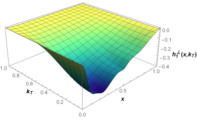
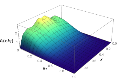
Figure 1: (left) The Boer-Mulders function generated by the non-perturbative kernel. (right) The unpolarized TMD $f_{1}$.

We first check the general constraint of positivity bound condition Bacchetta et al. (2000) using our TMDs

$$P\left(x,k_{\perp}\right)\equiv f_{1}\left(x,k_{\perp}\right)-\frac{k_{\perp}}{M_{\pi}}\left|h_{1}^{\perp}\left(x,k_{\perp}\right)\right|\geq 0.$$ (27)

In FIG. 2 we show that this constraint is mostly satisfied, with violations only occur for small $x$ at moderate and large $k_{T}$. We note that similar violations were reported in model studies Pasquini and Schweitzer (2014); Kotzinian (2008); Pasquini and Schweitzer (2011); Wang et al. (2017b) with the perturbative kernel. They indicate a limitation of current nonperturbative models to accurately capture the large $k_{T}$ behavior of the TMDs Ahmady et al. (2019). Fortunately, the violation is generally small in magnitude, and insignificant for $x\gtrsim 0.5$. This is compatible with the leading Fock state truncation we employ, which works better in the valence region.

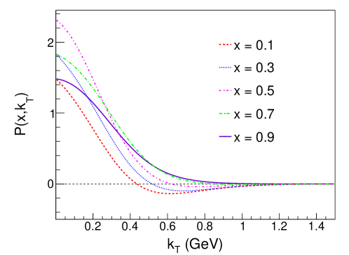
Figure 2: $P(x,k_{T})$ with the Boer-Mulders function generated by the non-perturbative kernel at $x=0.1$, $x=0.3$, $x=0.5$, $x=0.7$ and $x=0.9$.

IV The generalized Boer-Mulders shift

Parton distribution functions are defined within a certain regularization scheme at a given renormalization scale. At some low “hadronic scale” one deals with constituent (valence) degrees of freedom carrying the total hadron momentum: a constituent quark-antiquark pair in the pion case, or three constituent quarks in the nucleon case Pasquini and Schweitzer (2014). The results from phenomenological studies refer to an assumed low initial scale $\mu_{0}$. The value of $\mu_{0}$ is not known a $\bm{priori}$, but can be determined by comparing the $\langle x\rangle-$Mellin moment of pion valence PDF with experimental extraction or lattice prediction. In this work, the initial scale is set to be $\mu_{0}=0.5$ GeV. In the following we shall assume that theoretical uncertainties due to scheme dependence are smaller than the generic accuracy of LFWFs approaches.

In order to compare with lattice calculation, we evolve our TMDs from $\mu^{2}=\mu_{0}^{2}=0.25$ GeV² to $\mu^{2}=4.0$ GeV². The later scale corresponds to the Lattice simulation in Engelhardt et al. (2016). In the parton model, the collinear unpolarized PDF is related to the unpolarized TMD as

$$f_{1}(x)=\int\mathrm{d}^{2}\mathbf{k_{T}}f_{1}\left(x,k_{T}\right),$$ (28)

which denotes the original PDF of pion and satisfies the Dokshitzer-Gribov-Lipatov-Altarelli-Parisi (DGLAP) evolution Dokshitzer (1977); Gribov and Lipatov (1972); Altarelli and Parisi (1977). The first $k_{T}$-moment of Boer-Mulders function in pion is defined as Wang et al. (2017b)

$$h_{1\pi}^{\perp(1)}(x)=\int d^{2}\mathbf{k_{T}}\frac{\mathbf{k_{T}}^{2}}{2M_{\pi}^{2}}h_{1\pi}^{\perp}\left(x,{k_{T}}\right),$$ (29)

with the pion mass $M_{\pi}=130$ MeV. At the tree level, $h_{1\pi}^{\perp(1)q}(x)$ can be related to the twist-3 quark-gluon correlation function $T_{q,F}^{(\sigma)}(x,x)$ Wang et al. (2017b)

$$h_{1}^{\perp(1)q}(x)=\frac{1}{2M_{\pi}}T_{q,F}^{(\sigma)}(x,x),$$ (30)

whereas the QCD evolution for $T_{q,F}^{(\sigma)}(x,x)$ is given in Ref. Zhou et al. (2009); Kang and Qiu (2012).

To perform the DGLAP evolution on PDF $xf_{1}(x)$, we adopt the QCDNUM Botje (2011) package at leading order, and we choose the strong coupling constant as $\alpha_{s}(M_{Z}^{2})=0.118$. For the $h_{1}^{\perp(1)q}(x)$ case, we follow Ref. Wang et al. (2017b) and take the evolution kernel to be Wang et al. (2017b)

$$P_{qq}^{h_{1}^{\perp(1)}}(x)\approx\Delta_{T}P_{qq}(x)-N_{C}\delta(1-x),$$ (31)

with $\Delta_{T}P_{qq}(x)=C_{F}\left[\frac{2z}{(1-z)_{+}}+\frac{3}{2}\delta(1-x)\right]$. To describe the evolution of $xh_{1\pi}^{\perp(1)}(x)$, we also use the QCDNUM Botje (2011) program but insert the kernel (31) into the code. The numerical results are shown in FIG. 3. One can find that the peak of the evolved distribution shifts towards smaller $x$.

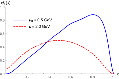
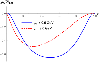
Figure 3: (left) Comparison of $xf_{1}(x)$ at two different scales $\mu_{0}=0.5$ GeV (blue solid) and $\mu=2.0$ GeV (red dashed). (right) Comparison of $xh_{1\pi}^{\perp(1)}(x)$ at two different scales $\mu_{0}=0.5$ GeV (blue solid) and $\mu=2.0$ GeV (red dashed).

On the other hand, the TMDs evolution is more complicated Collins (2013); Aybat and Rogers (2011). Taking the unpolarized TMD as an example, it is implemented in the space Fourier-conjugate to $k_{T}$

$$\widetilde{f}_{1}\left(x,b_{T}^{2};\mu\right)=\int_{0}^{\infty}dk_{T}k_{T}J_{0}\left(b_{T}k_{T}\right)f_{1}\left(x,k_{T}^{2};\mu\right).$$ (32)

The TMDs generally depend on two scales, the ultraviolet renormalization scale $\mu$ and the $\zeta$ that regulates the rapidity divergence. Here, we follow the evolution prescription in Bacchetta et al. (2017a) and set $\zeta=\mu$. The unpolarized TMD distribution in configuration space for a parton with flavor $a$ at a certain scale $\mu^{2}$ is written as Bacchetta et al. (2017a)

$$\tilde{f}_{1}^{a}\left(x,b_{T}^{2};\mu^{2}\right)= \sum_{i=q,\bar{q},g}\left(C_{a/i}\otimes f_{1}^{i}\right)\left(x,\bar{b}_{*},\mu_{b}^{2}\right)$$ (33)

$$\times e^{S\left(\mu_{b}^{2},\mu^{2}\right)}\left(\frac{\mu^{2}}{\mu_{b}^{2}}\right)^{-K\left(\bar{b}_{*};\mu_{b}\right)}\left(\frac{\mu^{2}}{\mu_{0}^{2}}\right)^{g_{K}\left(b_{T}\right)}\tilde{f}_{1\mathrm{NP}}^{a}\left(x,b_{T}^{2}\right),$$

The scale $\mu_{b}$ is

$$\mu_{b}=\frac{2e^{-\gamma_{E}}}{\bar{b}_{*}},$$ (34)

with $\gamma_{E}$ is the Euler constant and

$$\bar{b}_{*}\equiv\bar{b}_{*}\left(b_{T};b_{\min},b_{\max}\right)=b_{\max}\left(\frac{1-e^{-b_{T}^{4}/b_{\max}^{4}}}{1-e^{-b_{T}^{4}/b_{\min}^{4}}}\right)^{1/4}.$$ (35)

with

$$b_{\max}=2e^{-\gamma_{E}}/\mu_{0},\quad b_{\min}=2e^{-\gamma_{E}}/\mu.$$ (36)

The above choice guarantees that at the initial scale $\mu=\mu_{0}$ any effect of TMD evolution is absent. At leading order of $C_{a/i}$, the evolved TMD reduces to

$$\tilde{f}_{1}^{a}\left(x,b_{T}^{2};\mu^{2}\right)=f_{1}^{a}\left(x;\mu_{b}^{2}\right)e^{S\left(\mu_{b}^{2},\mu^{2}\right)}e^{\frac{1}{2}g_{K}\left(b_{T}\right)\ln\left(\mu^{2}/\mu_{0}^{2}\right)}\tilde{f}_{1\mathrm{NP}}^{a}\left(x,b_{T}^{2}\right),$$ (37)

where the Sudakov factor is Bacchetta et al. (2017b)

$$S\left(\mu_{b}^{2},\mu^{2}\right)=-\frac{1}{2}\int_{\mu_{b}^{2}}^{\mu^{2}}\frac{d\mu^{\prime 2}}{\mu^{\prime 2}}\left[A\left(\alpha_{S}\left(\mu^{\prime 2}\right)\right)\ln\left(\frac{\mu^{2}}{\mu^{\prime 2}}\right)+B\left(\alpha_{S}\left(\mu^{\prime 2}\right)\right)\right].$$ (38)

The functions $A$ and $B$ have a perturbative expansions of the form

$$A\left(\alpha_{S}\left(\mu^{2}\right)\right)=\sum_{k=1}^{\infty}A_{k}\left(\frac{\alpha_{S}}{\pi}\right)^{k},\quad B\left(\alpha_{S}\left(\mu^{2}\right)\right)=\sum_{k=1}^{\infty}B_{k}\left(\frac{\alpha_{S}}{\pi}\right)^{k}.$$ (39)

To NLL accuracy, one has Davies and Stirling (1984); Collins et al. (1985)

$$A_{1}=C_{F},\quad A_{2}=\frac{1}{2}C_{F}\left[C_{A}\left(\frac{67}{18}-\frac{\pi^{2}}{6}\right)-\frac{5}{9}N_{f}\right],\quad B_{1}=-\frac{3}{2}C_{F}.$$ (40)

Following Refs. Nadolsky et al. (2000); Landry et al. (2003); Konychev and Nadolsky (2006), the non-perturbative Sudakov factor in Eq. (37) is modeled as

$$g_{K}\left(b_{T}\right)=-g_{2}b_{T}^{2}/2,$$ (41)

with $g_{2}$ a free parameter. We choose $g_{2}\approx 0.13$ following the findings in Bacchetta et al. (2017a, b).

In addition to the Sudakov factors, the evolved TMD functions (37) are also related to two distribution functions, i.e., the collinear PDFs $f_{1}^{a}$ and the intrinsic nonperturbative part of the TMD $\tilde{f}_{1\mathrm{NP}}^{a}$. The former can be obtained by DGLAP evolution, and the latter can be determined from the condition that Eq. (37) reduces to our calculated TMDs at initial scale, as any evolution effect should be absent at $\mu=\mu_{b}=\mu_{0}$.

The evolution of pion’s Boer-Mulders function follows analogously. The Boer-Mulders function in the $b_{T}$-space is defined as Li et al. (2020)

$$\tilde{h}_{1,q/\pi}^{\perp\alpha}(x,b_{T};\mu)=\int d^{2}\mathbb{k_{T}}e^{-i\mathbb{k_{T}}\cdot\mathbb{b_{T}}}\frac{k_{T}^{\alpha}}{M_{\pi}}h_{1,q/\pi}^{\perp}\left(x,\mathbb{k}_{T}^{2};\mu\right).$$ (42)

For small $b_{T}$ and at leading order in $\alpha_{s}$, it can be expressed with twist-3 correlation function Collins et al. (1985); Bacchetta and Prokudin (2013); Li et al. (2020)

$$\tilde{h}_{1,q/\pi}^{\alpha\perp}(x,b_{T};\mu)=\left(\frac{-ib_{T}^{\alpha}}{2}\right)T_{q/\pi,F}^{(\sigma)}(x,x;\mu),.$$ (43)

From Eqs. (29), (30), one has Li et al. (2020)

$$T_{q/\pi,F}^{(\sigma)}(x,x;\mu)=\int d^{2}\mathbb{k_{T}}\frac{\mathbb{k_{T}}^{2}}{M_{\pi}}h_{1,q/\pi}^{\perp}\left(x,\mathbb{k_{T}}^{2};\mu\right)=2M_{\pi}h_{1,q/\pi}^{\perp(1)}.$$ (44)

Therefore, analogous to the unpolarized TMD in Eq. (37), the evolved Boer-Mulders function of the pion in $b_{T}$-space is

$$\tilde{h}_{1,q/\pi}^{\alpha\perp}(x,b_{T};\mu)=\left(\frac{-ib_{T}^{\alpha}}{2}\right)e^{S\left(\mu_{b}^{2},\mu^{2}\right)}e^{\frac{1}{2}g_{K}\left(b_{T}\right)\ln\left(\mu^{2}/\mu_{0}^{2}\right)}T_{q/\pi,F}^{(\sigma)}\left(x,x;\mu_{b}\right)\tilde{h}_{1,q/\pi,\mathrm{NP}}^{\alpha\perp}(x,b_{T}),$$ (45)

where $\tilde{h}_{1,q/\pi,\mathrm{NP}}^{\alpha\perp}(x,b_{T})$ is the intrinsic nonperturbative part of Boer-Mulders function. When $\mu=\mu_{0}$, the left hand side of Eq. (45) reduces to the calculated Boer-Mulders function at initial scale.

After evolving the TMDs in $b_{T}$-space, we Fourier transform the TMDs back to $k_{T}$ space. In FIG. 4, we show the unpolarized TMD and Boer-Mulders function of pion evolved to the scale of $\mu=2.0$ GeV. As compared to TMDs at hadronic scale in FIG.1, these TMDs shift toward lower $x$ and gets broader in $k_{T}$.

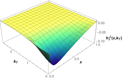
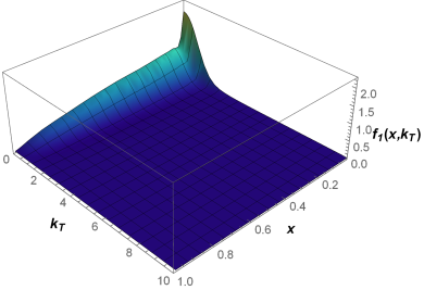
Figure 4: (left) The evolved Boer-Mulders function generated by the non-perturbative kernel at $\mu=2.0$ GeV. (right) The evolved unpolarized TMD $f_{1}$ at $\mu=2.0$ GeV.

Finally, we compare our results with lattice calculation, focusing on a quantity named the generalized Boer-Mulders shifts Engelhardt et al. (2016). For pion it has been predicted using a pion of mass $M_{\pi}=518$ MeV at the scale of 2 GeV Engelhardt et al. (2016), which is defined as

$$\left\langle k_{T}\right\rangle_{UT}\left(b_{T}^{2};\mu^{2}=4.0\ \mathrm{GeV}^{2}\right)=M_{\pi}\frac{\tilde{h}_{1,\pi}^{\perp[1](1)}\left(b_{T}^{2};\mu^{2}=4.0\ \mathrm{GeV}^{2}\right)}{\tilde{f}_{1,\pi}^{[1](0)}\left(b_{T}^{2};\mu^{2}=4.0\ \mathrm{GeV}^{2}\right)},$$ (46)

where the generalized TMD moments are given by

$$\tilde{f}^{[m](n)}\left(b_{T}^{2}\right)=\frac{2\pi n!}{M_{\pi}^{2n}}\int\mathrm{d}xx^{m-1}\int\mathrm{d}k_{T}k_{T}\left(\frac{k_{T}}{b_{T}}\right)^{n}J_{n}\left(b_{T}k_{T}\right)f\left(x,k_{T}^{2}\right),$$ (47)

and analogously for $\tilde{h}_{1,\pi}^{\perp[1](1)}$. The lattice prediction is displayed as the data points with error bars. Our result is shown in FIG. 5 as the purple dashed line. In addition, we also include the results from the NJL model Noguera and Scopetta (2015). We find that in NJL model, the results of $M_{\pi}=518$ MeV in approximately 0.8 times that of 140 MeV, as indicated by both evolutions Noguera and Scopetta (2015). Thus we multiply the purple curve by 0.8 and obtain the red dotted line as an estimate of pion mass variation effect. We find our results agree quite well with lattice calculation Engelhardt et al. (2016). Considering the uncertainty in the non-perturbative Sudakov factor, we test with different $g_{2}$ values in Eq. (41) and find the calculated generalized Boer-Mulders shift to be insensitive to $g_{2}$. This is reasonable as the ratio in Eq. (46) is devised to cancel the soft factors in the numerator and denominator.

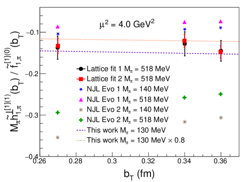
Figure 5: The generalized Boer-Mulders shift, Eq. (46), as a function of $b_{T}$. The results of NJL model include two types of evolution schemes, Evo 1 and 2, corresponding to different evolution factors (see Ref. Noguera and Scopetta (2015)). We indicate the generalized Boer-Mulders shift calculated using LFWFs, corresponding to pion mass $M_{\pi}=130$ with dashed line in the figure. The dotted line indicates the result of the dashed line multiplied by 0.8. Two sets of lattice data (Lattice fit 1 and 2), with their RMS deviation, obtained in Ref. Engelhardt et al. (2016) through independent fits, are shown for comparison.

V Conclusions

In this work, we study the unpolarized TMD and Boer-Mulders function of pion using DS-BSEs based LFWFs. The light front overlap representation is employed. To obtain a nonvanishing Boer-Mulders function, final-state interaction analysis is utilized to construct the gluons rescattering kernel $iG(x,q_{T})$, which incorporates the information of gauge link in SU(3) case. The two leading twist TMDs of pion at hadronic scale $\mu_{0}\approx 0.5$ GeV are thus given. We then evolve both TMDs to a higher scale of $2$ GeV. The generalized Boer-Mulders shift is found to be in good agreement with lattice prediction. We remark that at leading Fock-state, the Boer-Mulders function is proportional to the pion’s p-wave LF-LFWFs. Its emergence and magnitude is thus a reflection of the p-wave components inside pion, which essentially arises from the relativistic internal motion inside the pion. The DS-BSEs approach encapsulate such property, as well as QCD’s dynamical chiral symmetry breaking property, and pass them onto the DS-BSEs based LF-LFWFs, and eventually the pion TMDs.