VMA: Divide-and-Conquer Vectorized Map Annotation System for Large-Scale Driving Scene

Abstract

High-definition (HD) map serves as the essential infrastructure of autonomous driving. In this work, we build up a systematic vectorized map annotation framework (termed VMA) for efficiently generating HD map of large-scale driving scene. We design a divide-and-conquer annotation scheme to solve the spatial extensibility problem of HD map generation, and abstract map elements with a variety of geometric patterns as unified point sequence representation, which can be extended to most map elements in the driving scene. VMA is highly efficient and extensible, requiring negligible human effort, and flexible in terms of spatial scale and element type. We quantitatively and qualitatively validate the annotation performance on real-world urban and highway scenes, as well as NYC Planimetric Database. VMA can significantly improve map generation efficiency and require little human effort. On average VMA takes 160min for annotating a scene with a range of hundreds of meters, and reduces 52.3% of the human cost, showing great application value.

I Introduction

High-definition (HD) map contains a wide range of static map elements and encodes rich prior information of the driving scene, serving as the essential infrastructure of autonomous driving. However, map generation requires laborious human effort and high expenses, restricting the application and deployment of autonomous driving systems. In this work, we propose a systematic Vectorized Map Annotation (VMA) framework to improve the map generation efficiency of large-scale driving scenes.

VMA is highly extensible and flexible in terms of map element types. HD map is composed of diverse map elements with a variety of geometric patterns: line-shaped elements (road curb, lane divider, stop line, etc.), regular-shaped elements (arrow, speed bump, diamond marking, etc.), and closed-shaped regions (crosswalk, road intersection, diversion, etc.). Though some image processing methods [1, 2] and segmentation-based methods [3, 4, 5] can be integrated into the map generation pipeline for efficiency improvement, these existing methods can only tackle a small fraction of element types, and fail to model elements with rather complex geometric shapes. Differently, VMA models various map elements in a unified manner, i.e., map elements with different geometric patterns (line-shaped, regular-shaped and closed-shaped) are all generally abstracted as point sequence for automatic annotation. VMA unifies and simplifies the element representation. And this unified representation can be extended to most map elements in the driving scene, and is compatible with various map standards (like OpenDRIVE [6], Lanelet2 [7], and Apollo [8]).

Spatial extensibility is another key problem of map generation. On one hand, scaling up the spatial range of map is troublesome, due to memory and computation limitations. On the other hand, some map elements (e.g., road curb) have a long spatial coverage. Keeping the continuity and completeness of these elements is difficult. To solve the spatial extensibility problem, we design a divide-and-conquer annotation scheme and a vectorized merging algorithm, VMA has no restriction on the spatial range and is widely applicable.

An overview of the proposed framework is shown in Fig. 1. Specifically, VMA reconstructs the static scene through crowd-sourced multi-trip aggregation. Based on the reconstructed point cloud map (PCL map) and odometry information, VMA splits the scene into annotation units. We build up MapTR-based [9] Unit Annotator model, which takes unit PCL map as input and directly outputs unit vectorized map. Then vectorized map merging is performed to merge all unit vectorized maps into global vectorized map. Finally, point sparsification and human verification are performed to improve the annotation results.

VMA is highly automatic and significantly improves map generation efficiency. To validate the effectiveness, we apply VMA in both urban scene and highway scene. On average, VMA takes 160min for annotating a scene with a range of hundreds of meters and reduces 52.3% of the human cost. We also leverage VMA to perform lane boundary detection on NYC Planimetric Database for benchmark evaluation. VMA is of great application value in autonomous driving and can also be applied to other robotic scenarios.

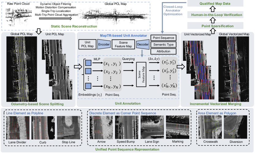
Figure 1: The VMA framework. VMA reconstructs the static scene through crowd-sourced multi-trip aggregation, and adopts a divide-and-conquer pipeline for scene annotation. VMA abstracts map elements with a variety of geometric patterns as unified point sequence representation for vectorized map annotation.

This paper’s contributions are summarized as follows:

• We design a divide-and-conquer annotation scheme to solve the spatial extensibility problem of HD map generation, and abstract map elements with a variety of geometric patterns as unified point sequence representation.

• Based on the unified map representation and divide-and-conquer annotation scheme, we build up a systematic vectorized map annotation framework (termed VMA) for automatically generating HD map of large-scale driving scenes. VMA is highly automatic and extensible, requiring negligible human effort, and flexible in terms of spatial scale and element type.

• We quantitatively and qualitatively validate the annotation performance on real-world urban and highway scenes, as well as NYC Planimetric Database. VMA can significantly improve map generation efficiency and require little human effort, showing great industrial application value.

The remaining part of the paper is organized as follows. A review of the related works on road marking extraction, line-shaped element extraction, online mapping, and lane detection is given in Section II. Section III describes the overall design of VMA, including unified point sequence representation, static scene reconstruction procedure, and divide-and-conquer scene annotation scheme. Experiments are presented in Section IV. And finally, conclusions and discussions are presented in Section V.

II Related Work

II-A Road Marking Extraction

Road markings are signs on road surfaces usually painted with highly retro-reflective materials, which make them noticeable to human vision and sensors of autonomous vehicles. Road markings are essential features of HD map because they provide rich traffic information (lane type, lane direction, etc.) for navigation. Traditionally, road marking extraction is achieved through image processing methods [1, 2], e.g., image denoising, image enhancement, edge-based detection, k-mean clustering, and regional growth. With the rapid development of deep learning, CNN-based methods have been widely employed in detecting and recognizing road markings. [10] predicts a semantic segmentation binary mask to distinguish lane markings from the background. [11] designs a wavelet-enhanced FCNN to segment high-resolution aerial imagery, and create a 3D reconstruction of road markings based on the least-squares line-fitting. [12] proposes a self-attention-guided capsule network, to extract road markings from aerial images. Different from these works, we model road marking as corner point sequence to achieve unified map element representation.

II-B Line-shaped Element Extraction

Existing methods for line-shaped element extraction can be divided into two kinds: segmentation-based methods [3, 4, 5] and iterative methods [13, 14, 15]. Segmentation-based methods predict segmentation probabilistic map from aerial images and then perform heuristic post-processing algorithms on the segmentation map to get the line-shaped map representation. DeepRoadMapper [3] segments the aerial images into interest categories, and connects the endpoint of the discontinued roads based on a specific distance threshold to alleviate the discontinuity issue of the road segmentation. [4] fixes the road network disconnectivity issue by predicting the orientation and segmentation of the road network and correcting the segmentation results with n-stacked multi-branch CNN. [5] adopts the encoder-decoder architecture as well as the attention mechanism, and introduces an edge detection algorithm to refine the segmented results. Iterative graph growing methods predict the map element in an auto-regressive manner (vertex by vertex). [13] designs a convolutional recurrent network to predict the road boundary. [14, 15] adopt better training strategy and graph growing policy to improve performance from the perspective of imitation learning. VMA models both line-shaped elements and road markings, as well as area elements, in a unified vectorized manner.

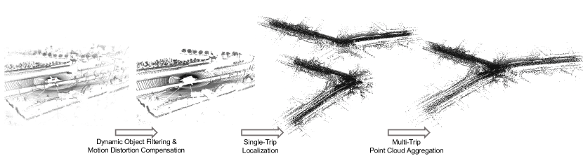
Figure 2: Static scene reconstruction. VMA generates dense point cloud map through crowd-sourced multi-trip aggregation.

II-C Online Mapping

Online mapping aims to create vehicle-centric local map on the fly and demands high efficiency. With the development of PV-to-BEV transformation [16], previous methods  [17, 18, 19, 20, 21, 22, 23] perform BEV semantic segmentation based on surround-view image data captured by vehicle-mounted cameras. To build vectorized semantic map, HDMapNet [24] adopts a segmentation-then-vectorization paradigm. To achieve end-to-end learning [25, 26, 27], VectorMapNet [28] adopts a coarse-to-fine two-stage pipeline and utilizes an auto-regressive decoder to predict points sequentially. MapTR [9] proposes permutation-equivalent modeling to exploit the undirected nature of semantic map and designs a parallel end-to-end framework. Online methods create vehicle-centric local map and focus on the balance of efficiency and accuracy. VMA aims at creating large-scale global map and focuses on map generation quality.

II-D Lane Detection

Lane detection [29, 30, 31, 32, 33, 34, 35, 36] is targeted at detecting lane elements in the scene. LaneATT [29] utilizes anchor-based deep lane detection model. LSTR [32] uses the Transformer architecture to output parameters of a lane shape model. GANet [30] formulates lane detection as a keypoint estimation and association problem and takes a bottom-up design. [31] performs 3D lane detection in BEV. BezierLaneNet [35] uses a fully convolutional network to predict 4-order Bezier lanes. PersFormer [36] proposes a Transformer-based architecture for spatial transformation and unifies 2D and 3D lane detection. VMA considers a wide range of map elements which include lane.

III Framework

The framework of VMA is depicted in Fig. 1. VMA first performs static scene reconstruction (Sec. III-A) and adopts a divide-and-conquer pipeline for scene annotation (Sec. III-B). The framework is highly automatic and requires little human effort.

III-A Static Scene Reconstruction

The static scene reconstruction procedure is mainly composed of multi-trip data collection, point cloud pre-processing (dynamic object filtering and motion distortion compensation), single-trip localization and mapping, and multi-trip point cloud aggregation (Fig. 2).

Multi-Trip Data Collection. The data collection vehicles are equipped with multi-modal sensors (GPS, IMU, wheel, LiDAR and camera). GPS, IMU, and wheel collect position and motion information. LiDAR generates point cloud map. Camera collects color and texture information of the scene and is equipped for map verification. The data collection procedure for a target scene is crowd-sourced and composed of several trips. On each trip, one vehicle takes a specific route travelling over the target scene. Different vehicles take different routes to fully cover the target scene.

Dynamic Object Filtering. Since the scene reconstruction of VMA includes temporal aggregation, the motion of traffic participants (vehicles, pedestrians, cyclists, etc.) may result in noisy points in the point cloud map. Thus, before aggregation, VMA adopts 3D detection algorithm [37] to mark out objects with 3D bounding box and filter out points inside the box for each LiDAR frame.

Motion Distortion Compensation. LiDAR sensor scans the environment in a rotational manner. A frame (sweep) of point cloud is composed of a set of scans at different timestamps of a rotation period. When the ego vehicle is moving, the pose of LiDAR sensor is continuously changing within each period. The scans of a frame are not aligned, resulting in motion distortion. Based on IMU pre-integration, the ego motion is estimated and the motion distortion is calculated to de-skew LiDAR point clouds.

Single-Trip Localization. In consideration of system efficiency, firstly the localization [38, 39, 40, 41, 42] process is independently and parallelly performed inside each trip. We adopt LIO-SAM [40] for single-trip offline localization. Specifically, initial odometry prior is generated through IMU pre-integration. Scan-matching [43] among LiDAR frames is used for odometry optimization. And GPS information is introduced to eliminate pose drift, which offers absolute pose measurements. Loop closure detection is performed to correct accumulated errors over time.

Multi-Trip Point Cloud Aggregation. The localization results of different trips are further jointly optimized through graph optimization [44, 45]. The pose at each timestamp of each trip is defined as node of graph. We adopt Scan-Context [46] as frame descripter for ICP, and obtain the relative pose between nodes of different trips. The relative pose of adjacent frames of the same trip is defined as the intra-trip edge, while the relative pose of two frames from two different trips is defined as the inter-trip edge. With the inter-trip and intra-trip edge constraints, we complete the overall pose graph optimization and get the optimized localization results. Based on the optimized localization results, all LiDAR frames are aligned for aggregation. The aggregated dense point cloud map covers the whole target scene, and contains rich semantic information for scene annotation.

III-B Divide-and-Conquer Scene Annotation

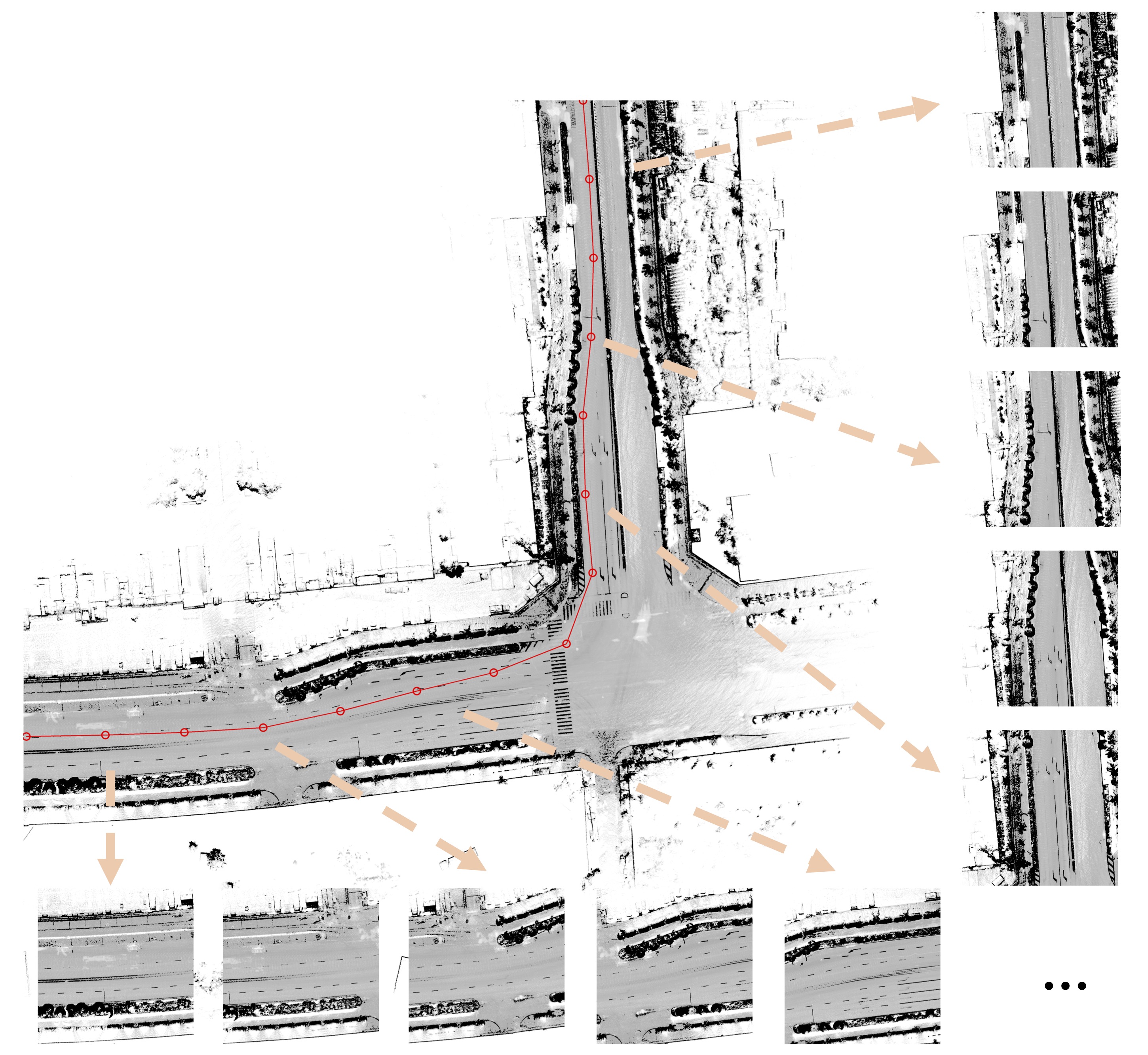
Figure 3: Scene splitting. Ego trajectory and sampled ego position are respectively marked with red line and dot.

VMA is targeted at annotating spatially unlimited large-scale scene, for which one-shot annotation is infeasible due to memory and computation limitations. Thus, a divide-and-conquer annotation scheme is designed to solve the spatial extensibility problem. Specifically, VMA splits the scene into overlapped annotation units, uses MapTR-based Unit Annotator to output the vectorized representation of map in each unit, and incrementally merges unit vectorized map to generate the global vectorized map.

Unified Point Sequence Representation. VMA abstracts a wide range of map element as unified point sequence representation. Based on the geometric characteristics, map element is categorized into three main types, i.e., line element, discrete element and area element (see Table I and Fig. 1).

Line elements mainly include road curb, lane divider, and stop line. Through sampling points at a fixed interval along the line, we get the corresponding point sequence representation $\{p_{i}\}^{N}$ ($N$ denotes the point number). By sequentially connecting these points, we get N-point polylines to represent line elements.

Discrete elements include all regular-shaped elements (like arrow, speed bump, and diamond marking), and is represented by the four corner points $\{p_{i}\}^{4}$ of the bounding box. The four points are ordered (front-left, front-right, back-right, and back left). The orientation of the element can be inferred from the order.

Area elements include closed-shaped regions, e.g., crosswalk, road intersection, diversion, etc. We frame the annotation of these regions as boundary regression, i.e., through sampling points at a fixed interval along the region’s boundary, we convert the boundary into an ordered point sequence $\{p_{i}\}^{N}$, which forms N-point polygons to represent the regions. We annotate the regions by detecting these points.

Table I: Geometric type, vectorized representation, semantic type, and attribution of map element in VMA. Map elements with different geometric patterns (line elements, discrete elements and area elements) are all abstracted as unified point sequence representation for vectorized map annotation. VMA also outputs attributions of map element.

Geometric Type	Vectorized Representation	Semantic Type	Attribution
Line Element	$N$-Point Sequence (Polyline)	Lane Divider	Direction: Unidirectional / Bidirectional; Line Type: Solid / Dotted / Fishbone; …
		Curb	Curb Type: Ground Side / Road Side / Guardrail
		Stop Line	-
		…	…
Discrete Element	Corner Point Sequence	Arrow	Arrow Type: Straight / Turn Off / Merge Right / No Turn Left / …; …
		Speed Bump	-
		Lane Sign	Lane Sign Type: Bike Lane / Bus Lane
		Marking	Marking Type: Diamond Marking / Inverted Triangle Marking
		…	…
Area Element	$N$-Point Sequence (Polygon)	Crosswalk	-
		Diversion	-
		…	…

Odometry-based Scene Splitting. VMA splits the scene into fixed-sized annotation units based on the odometry information (Sec. III-A). Specifically, as depicted in Fig. 3, along the vehicle’s trajectory, VMA samples ego positions at fixed time or distance intervals, denoted as $\mathbb{P}=\{\text{pos}_{1},\text{pos}_{2},...,\text{pos}_{n}\}$. Centered at these sampled positions, VMA crops unit PCL map from the global PCL map. And the scene is split into a group of annotation units along the ego trajectory.

Unit Annotation. We build up MapTR-based Unit Annotator model (see Fig. 1) which takes unit PCL map as input and directly outputs unit vectorized map. The unit PCL map is first sent into an encoder network, which flattens the unit PCL map into 2D map, extracts features with CNN, and outputs 2D scene feature map. Then a DETR-like [25, 9] decoder predicts map elements in a set-to-set manner. Each element corresponds to one sequence of learnable embeddings $\{e_{i}\}^{N}$ (one embedding for one point). Each embedding is sent into a MLP layer to predict point’s coordinate $(x,y)$ in the scene feature map. And then we sample features at $(x,y)$ of 2D scene feature map for predicting offsets $(\Delta x,\Delta y)$ to update $(x,y)$. Feature sampling and coordinate update are iteratively performed. Finally, the decoder outputs the point sequence represention of map element, as well as corresponding semantic type and attribution (see Table I).

The MapTR-based Unit Annotator is initially optimized with a small set of human-annotated scene data, and continuously optimized in a closed-loop manner (see Sec. 6). The human-annotated labels are converted to the vectorized point sequence representation for supervision. In the training phase, we perform one-to-one hierarchical assignment [9] between human-annotated elements and predicted elements. After one-to-one hierarchical assignment, the predicted point sequence is paired with the GT point sequence point by point (as depicted in Fig. 4, $P$ matches $Q$). Two kinds of supervision are adopted to constraint the geometry, p2l (point-to-line) and p2p (point-to-point) constraint. P2p constraint is the $L_{2}$ distance between paired points, while the P2l constraint is the point-to-line distance between predicted point $P$ and the two adjacent edges of $Q$. P2p constraint is applied to key points which require exact localization, i.e., the start and end points of line element, and corner points of discrete elements, while p2l constraint is applied to other points for adaptively keeping the geometry. When $L_{left}$ and $L_{right}$ are non-collinear, p2l constraint is equivalent to p2p constraint and makes $P$ converge to $Q$; when $L_{left}$ and $L_{right}$ are collinear, under the p2l constraint $P$ is not necessary to converge to $Q$ but is on the line. In this case, the convergence constraint is relaxed and also keeps the same geometry of element. Semantic type and attribution of each element are predicted by a MLP layer and supervised with cross-entropy loss.

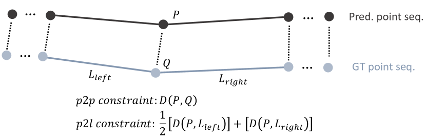
Figure 4: Geometric constraint of map element.

Incremental Vectorized Map Merging. MapTR-based Unit Annotator outputs unit vectorized map, consisting of fragmented map elements because of the unit border truncation. Incremental vectorized merging is performed to merge all unit vectorized maps $\{M^{i}_{local}\}$ into global vectorized map $M_{global}$. Concretely, based on the ego trajectory, unit vectorized maps are incrementally and sequentially merged:

$$M_{global}=(...(((M^{1}_{local}\oplus M^{2}_{local})\oplus M^{3}_{local})\oplus M^{4}_{local})...\oplus M^{n}_{local}),$$ (1)

where $\oplus$ denotes the merging process. The merging strategies vary according to the geometric patterns of map element:

• Line element (polyline): line elements are associated if the following conditions are met (refer to Fig. 5 (top)): two polylines overlap with each other; the overlapped length exceeds a threshold $\theta_{line}$; the endpoints of two polylines are close to the other polyline. We merge the associated elements (red one and yellow one) into one polyline (green one) by simply removing the overlapped part.

• Discrete element (corner point sequence). Chamfer distance $D_{chamfer}$ between two corner point sequences are calculated. If the distance is smaller than a threshold $\delta_{discrete}$, the two elements are associated. Through non-maximum suppression, associated elements are merged into one.

• Area element (polygon). If the IoU between two polygons exceeds a threshold $\delta_{area}$, the two polygons are associated. Associated polygons are merged into one polygon with the union operation (see Fig. 5 (bottom)).

• Attribution. The merging strategy of attribution is majority vote. The attribution of merged element is the majority of all associated elements.

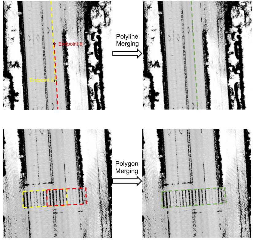
Figure 5: Illustration of merging strategies for line element (polyline) and area element (polygon).

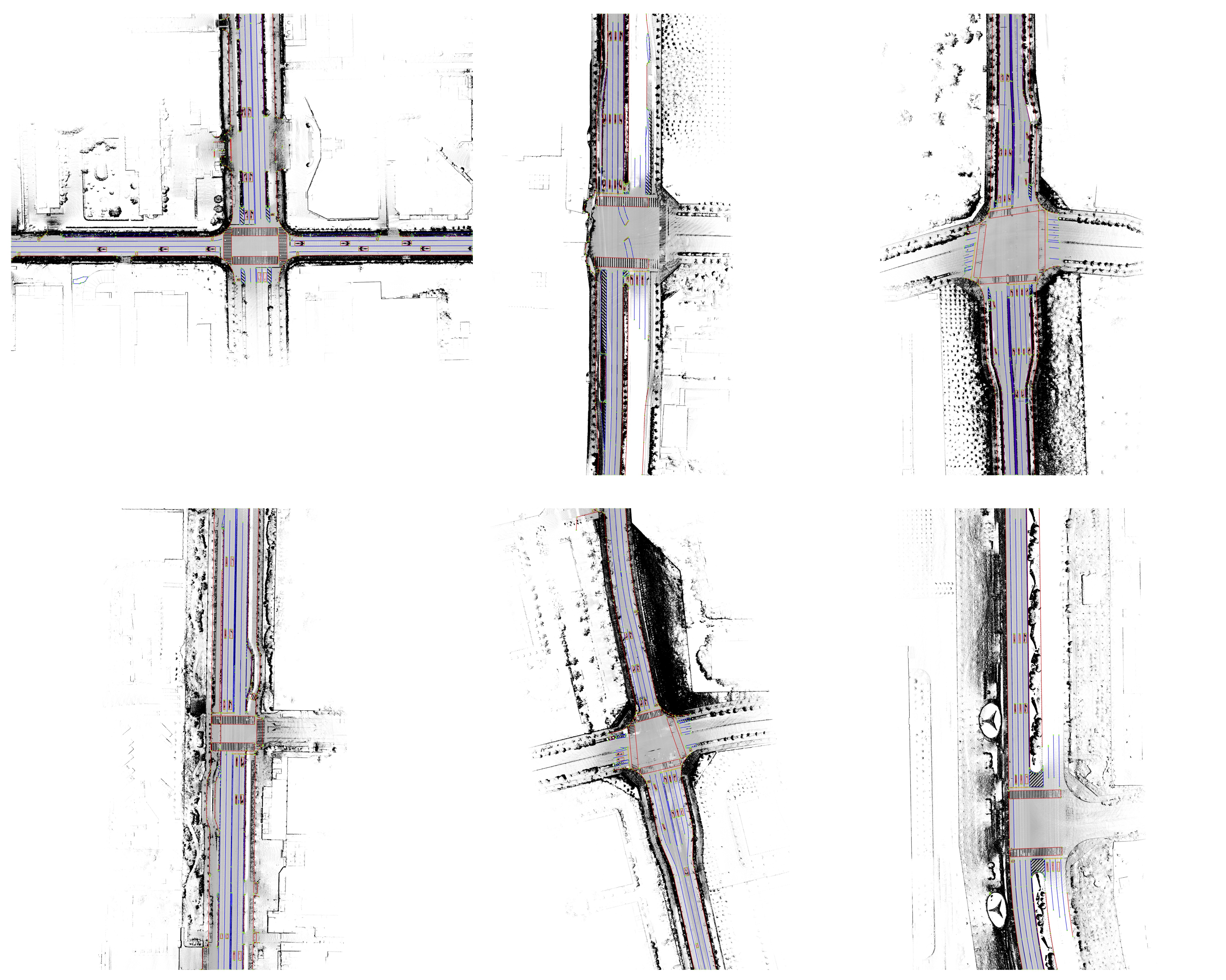
Figure 6: Automatic annotation results of urban scene. Zoon in for better view.

Point Sparsification. After incremental vectorized merging, fragmented map elements are transformed into complete map elements which are represented by dense and redundant point sequence. For the convenience of application and storage efficiency, VMA adopts the Douglas-Peucker algorithm to simplify the representation of map element, which iteratively removes points from the polyline (or polygon) while keeping the geomety.

Human-in-the-Loop Verification. Through the proposed divide-and-conquer scene annotation procedure, global vectorized map is obtained in a highly automatic manner. VMA introduces human verification for guaranteeing the annotation quality. After human verification, qualified vectorized map data are archived and regarded as extra training data for finetuning the MapTR-based Unit Annotator. With VMA running for a longer time, the annotation quality is continuously improved and less human effort is needed.

IV Experiments

IV-A Datasets

Real-World Urban Scene and Highway Scene. To validate the effectiveness of VMA, we apply VMA to map automatic annotation in both urban scene and highway scene. We collect a large amount of real-world scene data in a crowd-sourced way with the data collection vehicles equipped with multi-modal sensors. And the reported metrics are based on a validation set consisting of 850 urban scenes and 2082 highway scenes. 10231 urban scenes and 8334 highway scenes with map annotations are used to optimize the MapTR-based Unit Annotator.

NYC Planimetric Database. For fair comparisions with methods based on aerial images, following the Topo-boundary benchmark [15], we perform lane boundary detection on NYC Planimetric Database. NYC Planimetric Database contains 2147 high-resolution aerial images ($5000\times 5000$) with road-boundary annotations. Each pixel corresponds to $15.2cm$ in 3D space. According to the Topo-boundary benchmark [15], the high-resolution images are spilt into $1000\times 1000$ images for evaluation. More details about the benchmark setting are available in [15].

IV-B Experimental Settings

For line and area element, every instance corresponds to a 50-point sequence (i.e., $N=50$). We train the MapTR-based Unit Annotator of VMA on eight RTX 3090 GPUs with batch size 8. By default, the spatial range of annotation unit is $50m\times 50m$ for urban and highway scenes and $1000$ pixels $\times$ $1000$ pixels for NYC Planimetric Database. We use AdamW [47] optimizer and Cosine Annealing [48] scheduler with weight decay 0.01 and initial learning rate $2\times{10}^{-4}$.

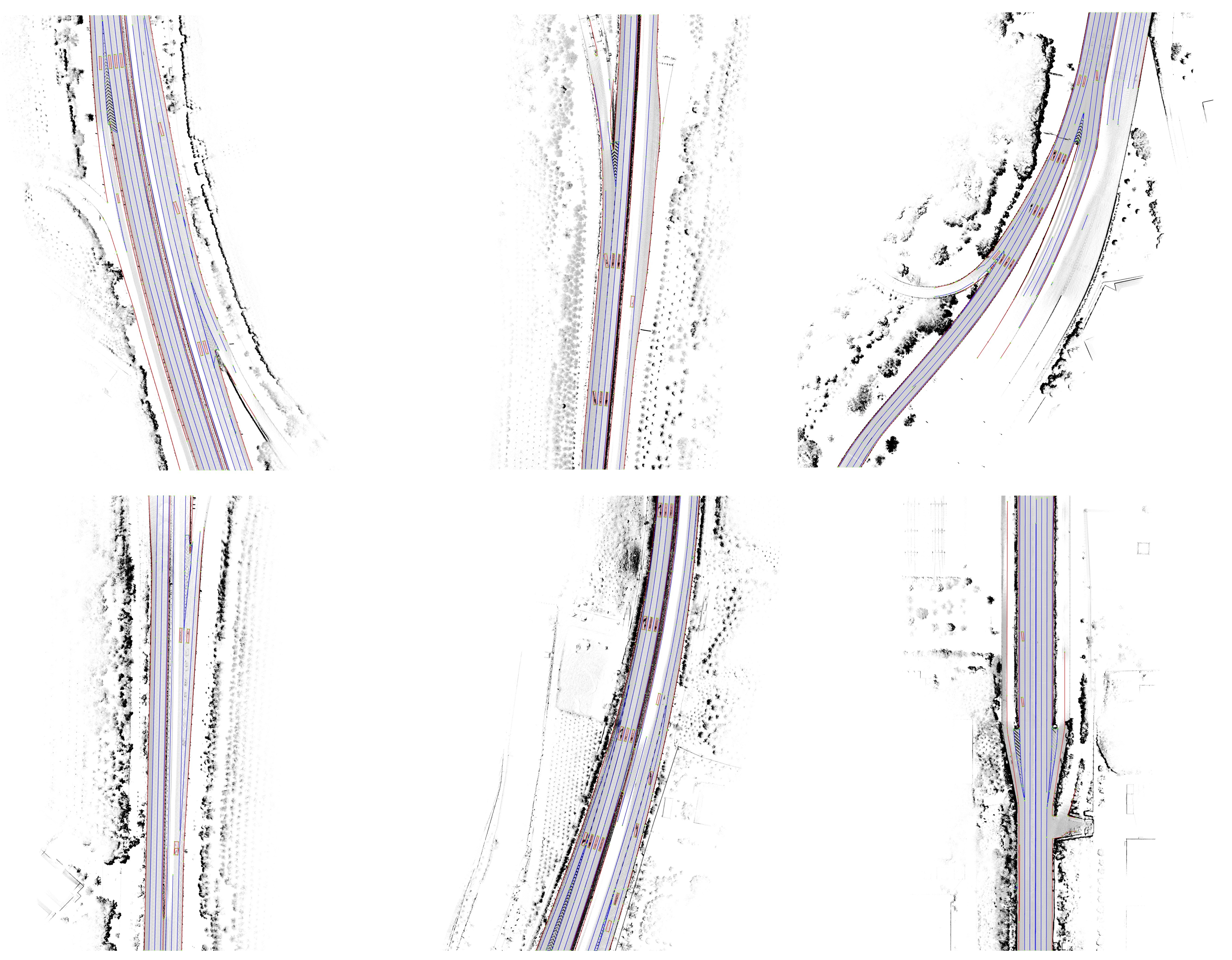
Figure 7: Automatic annotation results of highway scene. Zoon in for better view.

IV-C System Runtime

VMA is a highly automatic map annotation system. We present the detailed runtime of the system in Table II. For static scene reconstruction, the data collection is performed crowd-sourced way and approximately takes 30min per scene. Dynamic object filtering, single-trip localization, and multi-trip point cloud aggregation respectively takes 15min, 40min, and 60min per scene on average. Thanks to the divide-and-conquer scheme, the scene annotation procedure is quite efficient. Unit annotation is parallelly performed on GPU and costs little time. VMA requires negligible human effort (12min/scene averagely for map quality verification). And the overall runtime for annotating a scene (with a range of hundreds of meters) is 160min on average.

Table II: Detailed runtime of VMA.

Procedure	Sub-procedure	Time	Hardware
Scene Reconstruction	Data Collection	$\approx$ 30min/scene	-
	Dynamic Object Filtering	$\approx$ 15min/scene	GPU & CPU
	Motion Distortion Compensation	$\leq$ 1min/scene	CPU
	Single-Trip Localization	$\approx$ 40min/scene	CPU
	Multi-Trip Point Cloud Aggregation	$\approx$ 60min/scene	CPU
Scene Annotation	Scene Splitting	$\leq$ 1min/scene	CPU
	Unit Annotation	$\leq$ 1min/scene	GPU
	Vectorized Merging	$\leq$ 1min/scene	CPU
	Point Sparsification	$\leq$ 1min/scene	CPU
	Human Verification	$\approx$ 12min/scene	-
Overall	-	$\approx$160min/scene	-

Table III: Quantitative results on NYC Planimetric Database for comparison. The best results are highlighted in bold font. For all the metrics, larger values indicate better performance.

Methods	Precision $\uparrow$			Recall $\uparrow$			F1-score $\uparrow$			Naive $\uparrow$	APLS $\uparrow$	ECM $\uparrow$
	2 pixels	5 pixels	10 pixels	2 pixels	5 pixels	10 pixels	2 pixels	5 pixels	10 pixels
Seg.-then-skeleton. [14]	0.607	0.890	0.928	0.505	0.736	0.768	0.533	0.778	0.811	0.698	0.577	0.550
Deeproadmapper [3]	0.578	0.854	0.898	0.475	0.694	0.725	0.505	0.740	0.775	0.719	0.615	0.595
OrientationRefine [4]	0.620	0.878	0.913	0.602	0.850	0.884	0.605	0.855	0.888	0.797	0.750	0.756
RoadTracer [49]	0.391	0.707	0.791	0.416	0.743	0.821	0.399	0.718	0.798	0.869	0.739	0.824
VecRoad [50]	0.461	0.769	0.854	0.459	0.752	0.830	0.458	0.756	0.837	0.883	0.756	0.846
ConvBoundary [13]	0.510	0.845	0.934	0.455	0.692	0.752	0.465	0.737	0.805	0.958	0.671	0.786
DAGMapper [51]	0.407	0.751	0.868	0.353	0.649	0.747	0.371	0.684	0.787	0.896	0.679	0.758
iCurb [14]	0.550	0.833	0.890	0.538	0.815	0.873	0.542	0.820	0.877	0.910	0.826	0.889
Enhanced-iCurb [15]	0.560	0.839	0.894	0.542	0.811	0.864	0.549	0.821	0.874	0.925	0.822	0.893
VMA	0.533	0.872	0.935	0.530	0.856	0.913	0.528	0.858	0.916	0.900	0.865	0.901

IV-D Human Cost Comparison

As shown in Table LABEL:tab:humancost, on average, manual annotation requires 25min per scene. VMA requires 12min per scene and reduces 52.3% of the human cost.

Table IV: Human Cost Comparison.

Annotation Manner	Human Cost
Manual Annotation	$\approx$25min/scene
Auto Annotation w/ Verification (VMA)	$\approx$12min/scene

IV-E Qualitative Evaluation

Qualitative results of urban scene, highway scene, and NYC Planimetric Database are presented in Fig. 6, Fig. 7, and Fig. 8. VMA directly outputs high-quality global vectorized map for the whole scene, through a highly automatic divide-and-conquer scene annotation procedure. Human annotators only need to verify the automatic annotation results and adjust a small fraction of map elements. The map generation efficiency is significantly improved.

We can also observe some failed cases in Fig. 6 and Fig. 7. Specifically, if the point cloud map is not dense enough and the scene features are not rich enough, the map annotation quality is not satisfactory. The solution to this problem is increasing the trip number of data collection for better covering the target scene.

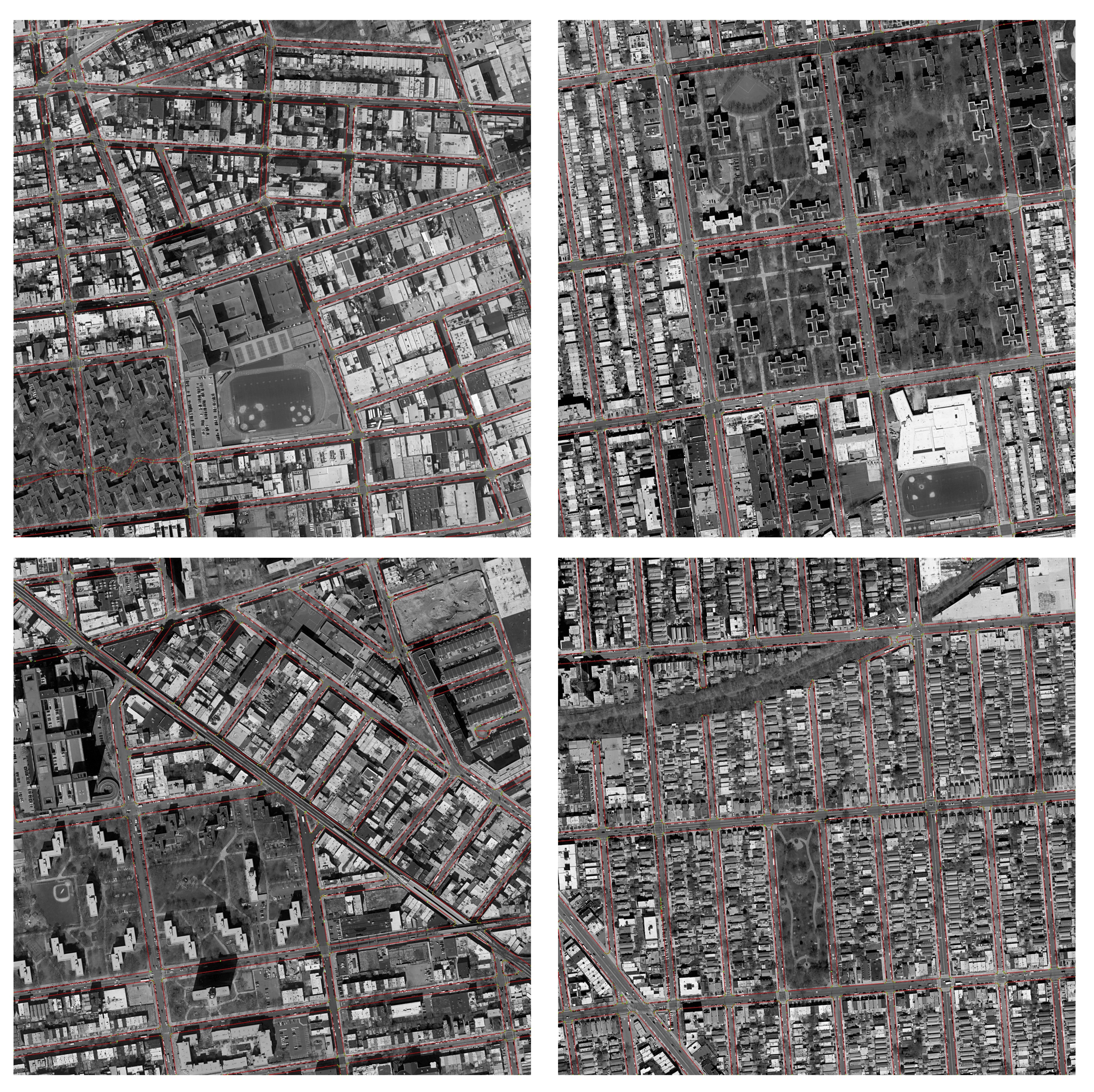
Figure 8: Automatic annotation results of NYC Planimetric Database. Zoon in for better view.

IV-F Quantitative Evaluation

We use the same metrics used in Topo-boundary benchmark [15] for quantitative comparison, which include pixel-level metrics (precision, recall, and F1-score), Naive Connectivity [13], APLS (Average Path Length Similarity) [52], and ECM (Entropy-based Connectivity) [15].

Pixel-level Metrics. Pixel-level metrics compose of precision, recall and F1-score. For pixel-level evaluation, predicted map elements and ground truth elements are firstly densified into rasterized representation. Suppose $P_{\text{pre}}$ is the densified pixel set of predicted map elements and $P_{\text{gt}}$ is the densified pixel set of ground truth map elements. Then, the Euclidean distance of every pixel pair between $P_{\text{pre}}$ and $P_{\text{gt}}$ are calculated. Denote $cd_{\text{pre}}$ as the chamfer distance of one predicted pixel to $P_{\text{gt}}$ and $cd_{\text{gt}}$ as the chamfer distance of one ground truth pixel to $P_{\text{pre}}$. Precision is the ratio of predicted pixels whose $cd_{\text{pre}}$ are smaller than preset threshold $\tau$ in all predicted pixels. Recall is the ratio of ground truth pixels whose $cd_{\text{gt}}$ are smaller than preset threshold $\tau$ in all ground truth pixels. The metrics are formulated as:

$$\text{Precision}=\frac{|\{p|d(p,P_{\text{gt}})<\tau,\forall p\in P_{\text{pre}}\}|}{|P_{\text{pre}}|},$$ (2)

$$\text{Recall}=\frac{|\{p|d(p,S_{\text{pre}})<\tau,\forall p\in P_{\text{gt}}\}|}{|P_{\text{gt}}|},$$

$$\text{F1-score}=\frac{2\cdot\text{Pecision}\cdot\text{Recall}}{\text{Precision}+\text{Recall}}.$$

Naive Connectivity. This metric measures the connectivity of predicted instance. Naive Connectivity uses the Hausdorff distance to match every predicted instance and ground-truth instance. Every predicted instance will be assigned to one ground-truth instance, according to the smallest Hausdorff distance. Multiple predicted instances could be assigned to one ground-truth instance. $M_{i}$ represents the number of predicted instances to which each true value is assigned. $C_{i}=\frac{1(M_{i}>0)}{M_{i}}$ is the connectivity of ground-truth, which means the short prediction of long ground-truth instance will be punished. The final result is the average sum of connectivity of each ground-truth instance.

APLS. APLS (Average Path Length Similarity) is proposed by [52] and has been widely used to evaluate topology correctness. It’s based on Dijkstra’s algorithm to measure the similarity of path.

Table V: Comparisons of training and inference time on NYC Planimetric Database.

Method	Training	Inference
Seg.-then-skeleton. [14]	0.45s/scene	0.33s/scene
Deeproadmapper [3]	1.32s/scene	1.57s/scene
OrientationRefine [4]	1.14s/scene	0.96s/scene
RoadTracer [49]	6.50s/scene	4.92s/scene
VecRoad [50]	19.89s/scene	14.17s/scene
ConvBoundary [13]	17.47s/scene	25.17s/scene
DAGMapper [51]	8.19s/scene	4.92s/scene
iCurb [14]	6.74s/scene	3.11s/scene
Enhanced-iCurb [15]	7.25s/scene	2.38s/scene
VMA	0.35s/scene	0.11s/scene

ECM. Naive Connectivity ignores the length of predicted instances. ECM (Entropy-based Connectivity) metric is used in [15], which assigns predicted longer instances with higher weight in the metric. ECM is formulated as:

$$ECM=\sum_{i=1}^{N}\alpha_{i}e^{-C_{i}},$$ (3)

$$C_{i}=\sum_{j=1}^{M_{i}}-p_{j}log(p_{j}),$$

$$p_{j}=\frac{\text{length}(G^{j}_{\text{pre}})}{\sum_{I\in S_{i}}\text{length}(I)}.$$

In ECM, Hausdorff distance matching is replaced with pixel-level voting mechanism. Each pixel of predicted instance votes ground-truth instance with the closest Euclidean distance, and the predicted instance will be assigned to ground-truth instance with the most votes. And the connectivity value $C_{i}$ is calculated from the entropy of dominance value. $S_{i}$ is the set of all predicted instances assigned to one ground truth $G^{i}_{\text{gt}}$. Dominance value $p_{j}$ is the ratio of the length of predicted instance $G^{j}_{\text{pre}}$ to the sum of the length of all the instance in $S_{i}$. $M_{i}$ is the number of $S_{i}$. $\alpha_{i}$ is the completion of $G_{gt}^{i}$, which is equal to the sum of the length of assigned instances in $G_{pre}$ projected onto $G_{gt}^{i}$ divided by the length of $G_{gt}^{i}$.

Quantitative comparisons on NYC Planimetric Database are presented in Table LABEL:tab:NYC. VMA achieves the best results in terms of most metrics. Besides, VMA is efficient in both training and inference phase (on average 0.35s/scene for training and 0.11s/scene for inference), as shown in Table LABEL:tab:NYC.

Quantitative evaluations of urban scene are presented in Table LABEL:tab:urban. For all types of map elements, even under the strict distance threshold $0.30m$, VMA achieves high recall, precision, and F1-score. It shows the unified point sequence representation well models map elements with various geometric patterns. Especially for lane divider and curb, which are the most important map elements of the driving scene, recall$@0.30m$, precision$@0.30m$, and F1-score$@0.30m$ all exceed $0.90$. Some infrequent elements (like speed bump) correspond to limited training samples. With the training samples accumulated and the closed-loop annotator optimization, the annotation quality can be continuously improved.

Quantitative evaluations of highway scene are presented in Table LABEL:tab:highway. The metrics of the highway scene are much higher than those of the urban scene. The highway scene is standardized and easy to annotate, while the urban scene is more complex and includes a large number of intersection scenarios. This difference accounts for the gap of metrics.

Annotation accuracy of attributions is shown in Table VIII. Attribution predictions of VMA are quite accurate, requiring little human effort for correction.

Table VI: Quantitative results of urban scene.

Semantic Type	Precision $\uparrow$			Recall $\uparrow$			F1-score $\uparrow$
	0.30m	0.75m	1.50m	0.30m	0.75m	1.50m	0.30m	0.75m	1.50m
Lane Divider	0.913	0.926	0.932	0.930	0.937	0.940	0.915	0.925	0.930
Curb	0.910	0.929	0.939	0.917	0.934	0.941	0.906	0.924	0.933
Stop Line	0.780	0.886	0.922	0.780	0.887	0.918	0.767	0.874	0.907
Arrow	0.764	0.857	0.870	0.810	0.908	0.919	0.769	0.862	0.873
Speed Bump	0.632	0.828	0.883	0.626	0.806	0.860	0.607	0.795	0.850
Lane Sign	0.682	0.934	0.951	0.651	0.904	0.926	0.652	0.900	0.919
Marking	0.799	0.913	0.926	0.777	0.883	0.899	0.773	0.880	0.899
Crosswalk	0.559	0.720	0.810	0.616	0.797	0.893	0.570	0.736	0.827
Diversion	0.581	0.722	0.811	0.647	0.808	0.904	0.596	0.742	0.832
Average	0.736	0.879	0.894	0.750	0.873	0.911	0.728	0.847	0.886

Table VII: Quantitative results of highway scene.

Semantic Type	Precision $\uparrow$			Recall $\uparrow$			F1-score $\uparrow$
	0.30m	0.75m	1.50m	0.30m	0.75m	1.50m	0.30m	0.75m	1.50m
Lane Divider	0.934	0.940	0.944	0.948	0.953	0.955	0.935	0.941	0.944
Curb	0.882	0.912	0.925	0.910	0.937	0.948	0.887	0.916	0.928
Stop Line	0.802	0.903	0.932	0.793	0.897	0.925	0.788	0.890	0.918
Arrow	0.860	0.955	0.967	0.855	0.949	0.961	0.852	0.945	0.957
Speed Bump	0.694	0.866	0.906	0.648	0.841	0.889	0.654	0.837	0.882
Lane Sign	0.849	0.962	0.969	0.828	0.936	0.946	0.829	0.938	0.947
Marking	0.919	0.981	0.988	0.913	0.973	0.982	0.913	0.973	0.982
Crosswalk	0.685	0.831	0.927	0.677	0.821	0.913	0.673	0.816	0.910
Diversion	0.700	0.834	0.924	0.699	0.827	0.913	0.690	0.820	0.908
Average	0.814	0.909	0.932	0.808	0.904	0.936	0.802	0.897	0.931

Table VIII: Annotation accuracy of attributions.

Attribution	Tag	Accuracy (%)
Lane Direction	Unidirectional / Bidirectional	99.8
Lane Type	Solid / Dotted / Fishbone	99.3
Lane Property	General / Stay / Tide / Bus / Three Color	99.6
Lane Flag	Single / Double / Triple	99.3
Lane Width	Normal / Wide	99.8
Curb Type	Ground Side / Road Side / Guardrail	91.6
Arrow Direction	Straight / Turn Off / Merge Right / No Turn Left / …	98.1
Lane Sign Type	Bike Lane / Bus Lane	100.0
Marking Type	Diamond Marking / Inverted Triangle Marking	92.6

V Conclusion and Discussion

We present VMA, a vectorized map annotation framework based on the unified map representation and the divide-and-conquer annotation scheme. VMA is highly automatic and extensible, requiring negligible human effort and flexible in terms of spatial scale and element type. VMA can significantly improve the map generation efficiency and require little human effort, showing great industrial application value. We find that the quality of scene reconstruction affects the annotation quality a lot. By introducing more sensor information (like camera and RADAR) for scene reconstruction, VMA can be further enhanced. And the divide-and-conquer scheme of VMA can also be extended to large-scale lane graph construction based on LaneGAP [53]. We leave these as future work.

References

- [1] J. Canny, “A computational approach to edge detection,” TPAMI, 1986.
- [2] Z. Zhang, X. Zhang, S. Yang, and J. Yang, “Research on pavement marking recognition and extraction method,” 2021.
- [3] G. Máttyus, W. Luo, and R. Urtasun, “Deeproadmapper: Extracting road topology from aerial images,” in ICCV, 2017.
- [4] A. Batra, S. Singh, G. Pang, S. Basu, C. Jawahar, and M. Paluri, “Improved road connectivity by joint learning of orientation and segmentation,” in CVPR, 2019.
- [5] H. Ghandorh, W. Boulila, S. Masood, A. Koubaa, F. Ahmed, and J. Ahmad, “Semantic segmentation and edge detection - approach to road detection in very high resolution satellite images,” Remote. Sens., 2022.
- [6] “Asam opendrive,” https://www.asam.net/standards/detail/opendrive/.
- [7] F. Poggenhans, J. Pauls, J. Janosovits, S. Orf, M. Naumann, F. Kuhnt, and M. Mayr, “Lanelet2: A high-definition map framework for the future of automated driving,” in ITSC, W. Zhang, A. M. Bayen, J. J. S. Medina, and M. J. Barth, Eds., 2018.
- [8] “Apollo map,” https://github.com/ApolloAuto/apollo/tree/master/modules/map.
- [9] B. Liao, S. Chen, X. Wang, T. Cheng, Q. Zhang, W. Liu, and C. Huang, “Maptr: Structured modeling and learning for online vectorized hd map construction,” in ICLR, 2023.
- [10] S. M. Azimi, P. Fischer, M. Körner, and P. Reinartz, “Aerial lanenet: Lane-marking semantic segmentation in aerial imagery using wavelet-enhanced cost-sensitive symmetric fully convolutional neural networks,” IEEE Trans. Geosci. Remote. Sens., 2019.
- [11] F. Kurz, S. M. Azimi, C. Sheu, and P. d’Angelo, “Deep learning segmentation and 3d reconstruction of road markings using multiview aerial imagery,” ISPRS Int. J. Geo Inf., 2019.
- [12] Y. Yu, Y. Li, C. Liu, J. Wang, C. Yu, X. Jiang, L. Wang, Z. Liu, and Y. Zhang, “Markcapsnet: Road marking extraction from aerial images using self-attention-guided capsule network,” IEEE Geosci. Remote. Sens. Lett., 2022.
- [13] J. Liang, N. Homayounfar, W.-C. Ma, S. Wang, and R. Urtasun, “Convolutional recurrent network for road boundary extraction,” in CVPR, 2019.
- [14] Z. Xu, Y. Sun, and M. Liu, “icurb: Imitation learning-based detection of road curbs using aerial images for autonomous driving,” RA-L, 2021.
- [15] ——, “Topo-boundary: A benchmark dataset on topological road-boundary detection using aerial images for autonomous driving,” RA-L, 2021.
- [16] Y. Ma, T. Wang, X. Bai, H. Yang, Y. Hou, Y. Wang, Y. Qiao, R. Yang, D. Manocha, and X. Zhu, “Vision-centric bev perception: A survey,” arXiv preprint arXiv:2208.02797, 2022.
- [17] Z. Liu, S. Chen, X. Guo, X. Wang, T. Cheng, H. Zhu, Q. Zhang, W. Liu, and Y. Zhang, “Vision-based uneven bev representation learning with polar rasterization and surface estimation,” arXiv preprint arXiv:2207.01878, 2022.
- [18] B. Zhou and P. Krähenbühl, “Cross-view transformers for real-time map-view semantic segmentation,” in CVPR, 2022.
- [19] Z. Li, W. Wang, H. Li, E. Xie, C. Sima, T. Lu, Y. Qiao, and J. Dai, “Bevformer: Learning bird’s-eye-view representation from multi-camera images via spatiotemporal transformers,” in ECCV, 2022.
- [20] Z. Liu, H. Tang, A. Amini, X. Yang, H. Mao, D. Rus, and S. Han, “Bevfusion: Multi-task multi-sensor fusion with unified bird’s-eye view representation,” arXiv preprint arXiv:2205.13542, 2022.
- [21] Y. Liu, J. Yan, F. Jia, S. Li, Q. Gao, T. Wang, X. Zhang, and J. Sun, “Petrv2: A unified framework for 3d perception from multi-camera images,” arXiv preprint arXiv:2206.01256, 2022.
- [22] J. Lu, Z. Zhou, X. Zhu, H. Xu, and L. Zhang, “Learning ego 3d representation as ray tracing,” in ECCV, 2022.
- [23] S. Chen, T. Cheng, X. Wang, W. Meng, Q. Zhang, and W. Liu, “Efficient and robust 2d-to-bev representation learning via geometry-guided kernel transformer,” arXiv preprint arXiv:2206.04584, 2022.
- [24] Q. Li, Y. Wang, Y. Wang, and H. Zhao, “Hdmapnet: An online hd map construction and evaluation framework,” in ICRA, 2022.
- [25] N. Carion, F. Massa, G. Synnaeve, N. Usunier, A. Kirillov, and S. Zagoruyko, “End-to-end object detection with transformers,” in ECCV, 2020.
- [26] X. Zhu, W. Su, L. Lu, B. Li, X. Wang, and J. Dai, “Deformable DETR: deformable transformers for end-to-end object detection,” in ICLR, 2021.
- [27] Y. Fang, B. Liao, X. Wang, J. Fang, J. Qi, R. Wu, J. Niu, and W. Liu, “You only look at one sequence: Rethinking transformer in vision through object detection,” NeurIPS, 2021.
- [28] Y. Liu, Y. Wang, Y. Wang, and H. Zhao, “Vectormapnet: End-to-end vectorized hd map learning,” arXiv preprint arXiv:2206.08920, 2022.
- [29] L. Tabelini, R. Berriel, T. M. Paixao, C. Badue, A. F. De Souza, and T. Oliveira-Santos, “Keep your eyes on the lane: Real-time attention-guided lane detection,” in CVPR, 2021.
- [30] J. Wang, Y. Ma, S. Huang, T. Hui, F. Wang, C. Qian, and T. Zhang, “A keypoint-based global association network for lane detection,” in CVPR, 2022.
- [31] N. Garnett, R. Cohen, T. Pe’er, R. Lahav, and D. Levi, “3d-lanenet: end-to-end 3d multiple lane detection,” in ICCV, 2019.
- [32] R. Liu, Z. Yuan, T. Liu, and Z. Xiong, “End-to-end lane shape prediction with transformers,” in WACV, 2021.
- [33] Y. Guo, G. Chen, P. Zhao, W. Zhang, J. Miao, J. Wang, and T. E. Choe, “Gen-lanenet: A generalized and scalable approach for 3d lane detection,” in ECCV, 2020.
- [34] R. Liu, D. Chen, T. Liu, Z. Xiong, and Z. Yuan, “Learning to predict 3d lane shape and camera pose from a single image via geometry constraints,” in AAAI, 2022.
- [35] Z. Feng, S. Guo, X. Tan, K. Xu, M. Wang, and L. Ma, “Rethinking efficient lane detection via curve modeling,” in CVPR, 2022.
- [36] L. Chen, C. Sima, Y. Li, Z. Zheng, J. Xu, X. Geng, H. Li, C. He, J. Shi, Y. Qiao, and J. Yan, “Persformer: 3d lane detection via perspective transformer and the openlane benchmark,” in ECCV, 2022.
- [37] Y. Hu, Z. Ding, R. Ge, W. Shao, L. Huang, K. Li, and Q. Liu, “Afdetv2: Rethinking the necessity of the second stage for object detection from point clouds,” in AAAI, 2022.
- [38] J. Zhang and S. Singh, “LOAM: lidar odometry and mapping in real-time,” in Robotics: Science and Systems X, University of California, 2014.
- [39] T. Shan and B. Englot, “Lego-loam: Lightweight and ground-optimized lidar odometry and mapping on variable terrain,” in IROS, 2018.
- [40] T. Shan, B. J. Englot, D. Meyers, W. Wang, C. Ratti, and D. Rus, “LIO-SAM: tightly-coupled lidar inertial odometry via smoothing and mapping,” in IROS, 2020.
- [41] H. Yin, S. Li, Y. Tao, J. Guo, and B. Huang, “Dynam-slam: An accurate, robust stereo visual-inertial SLAM method in dynamic environments,” T-RO, 2023.
- [42] R. Mur-Artal, J. M. M. Montiel, and J. D. Tardós, “ORB-SLAM: A versatile and accurate monocular SLAM system,” T-RO, 2015.
- [43] A. Segal, D. Haehnel, and S. Thrun, “Generalized-icp.” in Robotics: science and systems, 2009.
- [44] G. Kim and A. Kim, “Lt-mapper: A modular framework for lidar-based lifelong mapping,” in ICRA, 2022.
- [45] S. Yang, X. Zhu, X. Nian, L. Feng, X. Qu, and T. Ma, “A robust pose graph approach for city scale lidar mapping,” in IROS, 2018.
- [46] “Scan context: Egocentric spatial descriptor for place recognition within 3d point cloud map,” in IROS, 2018.
- [47] I. Loshchilov and F. Hutter, “Decoupled weight decay regularization,” arXiv preprint arXiv:1711.05101, 2017.
- [48] ——, “Sgdr: Stochastic gradient descent with warm restarts,” arXiv preprint arXiv:1608.03983, 2016.
- [49] F. Bastani, S. He, S. Abbar, M. Alizadeh, H. Balakrishnan, S. Chawla, S. Madden, and D. DeWitt, “Roadtracer: Automatic extraction of road networks from aerial images,” in CVPR, 2018.
- [50] Y.-Q. Tan, S.-H. Gao, X.-Y. Li, M.-M. Cheng, and B. Ren, “Vecroad: Point-based iterative graph exploration for road graphs extraction,” in CVPR, 2020.
- [51] N. Homayounfar, W.-C. Ma, J. Liang, X. Wu, J. Fan, and R. Urtasun, “Dagmapper: Learning to map by discovering lane topology,” in ICCV, 2019.
- [52] A. V. Etten, D. Lindenbaum, and T. M. Bacastow, “Spacenet: A remote sensing dataset and challenge series,” arXiv preprint arXiv:1807.01232, 2018.
- [53] B. Liao, S. Chen, B. Jiang, T. Cheng, Q. Zhang, W. Liu, C. Huang, and X. Wang, “Lane graph as path: Continuity-preserving path-wise modeling for online lane graph construction,” arXiv preprint arXiv:2303.08815, 2023.