Novel charged black hole solutions of Born-Infeld type:
General properties, Smarr formula and Quasinormal frequencies

Abstract

We investigate two novel models of charged black holes in the framework of non-linear electrodynamics of Born-Infeld type. In particular, starting from two concrete Lagrangian densities, the corresponding metric potentials, the electric field, the Smarr formula and finally, the (scalar) quasinormal modes are computed for each model. Our findings show that although the models look very similar, their quasinormal spectra are characterized by certain differences.

I Introduction

Non-linear Electrodynamics (NLE), with already a long history, has attracted a lot of attention, and it has been extensively studied over the years. To begin with, one may mention that classical electrodynamics, i.e. Maxwell’s theory, consists of a system of linear equations. At quantum level, however, as soon as radiative corrections are taken into account, the effective field equations become non-linear. The very first works go back to the 30’s, when Euler and Heisenberg managed to obtain corrections within quantum electrodynamics Euler , while Born and Infeld were able to obtain a finite self-energy of point-like charges BI . Born-Infeld theory has inspired other models of NLE, for example the theory of Soleng soleng and others, such as those presented in Refs. Kruglov:2014hpa ; Kruglov:2016cdm ; Kruglov:2017fuj ; Kruglov:2017xmb ; Gaete:2017cpc ; Gaete:2018nwq ; Mazharimousavi:2019sgz ; Mazharimousavi:2021uki ; Gullu:2020ant ; Bandos:2020jsw ; Kruglov:2021bhs ; Belmar-Herrera:2022ebd . They all characterized by a non-linear parameter $b$, and in a certain limit ($b\rightarrow 0$ or $b\rightarrow\infty$, depending on the formulation) the standard Reissner-Nordström solution RN of Maxwell’s linear theory is recovered. Thus, as already mentioned, Born and Infeld introduced non-linear electrodynamics to avoid divergences obtaining a finite self-energy of a point-like charge. For two decades, the Born-Infeld action was extensively studied in the context of Superstring Theory, where the dynamics of D-branes, solitonic solutions of Supergravity, are described by the corresponding Born-Infeld action. In this sense, the replacement of the well-known Reissner-Nordstrom black hole solutions (in Einstein-Maxwell theory) to the charged black hole solutions (in Einstein-Born-Infeld theory) has motivated several investigations, for example, see Aiello:2004rz ; Dey:2004yt . More importantly, albeit we have a vast list of non-linear electrodynamics black hole solutions, many of them still maintain the singularity problem and just offer a more intricate solution, different from the Born-Infeld black hole solution where a non-divergent electric field is obtained. Additional works on non-linear electrodynamics and their properties can be found in Kanzi:2020cyv ; Jafarzade:2020ova ; Pourhassan:2022cvn ; deOliveira:1994in ; Javed:2022psa ; Kumaran:2022soh ; Okyay:2021nnh ; Javed:2019kon .

Moreover, a generalization of Maxwell’s theory leads to the so called Einstein-power-Maxwell (EpM) theory EpM1 ; EpM2 ; EpM3 ; EpM4 ; EpM5 ; EpM6 ; EpM7 ; EpM8 ; EpM9 ; EpM10 ; EpM11 ; Hassaine:2008pw ; Gonzalez:2009nn , described by a power-law where the Lagrangian density is of the form $\mathcal{L}(F)=F^{k}$, with $F$ being the Maxwell invariant, and where $k$ is an arbitrary rational number. The advantage of EpM theories is that they preserve the nice properties of conformal invariance in any number of space-time dimensionality $D$, as long as $k=D/4$, since it is easy to verify that for that choice of $k$ the corresponding stress-energy tensor is trace-less. Furthermore, considering appropriate non-linear sources, which in the weak field limit boil down to Maxwell’s theory, one may generate new solutions (Bardeen-like solutions Bardeen , see also borde ) to Einstein’s field equations beato1 ; beato2 ; beato3 ; bronnikov ; dymnikova ; hayward ; vagenas1 ; vagenas2 ; Rodrigues:2017yry . Those new solutions possess an event horizon, while at the same time their curvature invariants are regular everywhere. This is to be contrasted to the standard Reissner-Nordström solution of Einstein-Maxwell theory, where a singularity at the origin, $r\rightarrow 0$, is present.

Black holes are a robust prediction of Einstein’s General Relativity GR . They are fascinating objects of paramount importance both for classical and quantum gravity. Over the last years, after the first image of the black hole shadow by the Event Horizon Telescope EHT , together with the historical first direct detection of gravitational waves from a black hole merger in binaries by the LIGO/VIRGO collaborations GWs , we have been convinced that black holes do exist in Nature. Static, spherically symmetric black hole solutions with a net electric charge $Q$ and mass $M$ within linear or non-linear electrodynamics have thermal properties, just like ordinary thermodynamic systems, and they obey the four laws of black hole thermodynamics Bardeen:1973gs , which are very similar to the usual four laws of statistical mechanics. In particular, black hole solutions have a Hawking temperature, $T_{H}$, and a Bekenstein entropy, $S$, given by hawking1 ; hawking2 ; bekenstein

$$T_{H}=\frac{1}{4\pi}\>f^{\prime}(r_{h}),\;\;\;\;S=\frac{A_{h}}{4}=\pi r_{h}^{2}$$ (1)

where $r_{h}$ is the event horizon, $f(r)$ is the lapse function, $r$ is the radial coordinate, and $A_{h}=4\pi r_{h}^{2}$ is the horizon area for solutions with a spherical horizon topology. Moreover, one may derive a Smarr formula smarr using Euler’s theorem for homogeneous functions. Within Maxwell’s linear electrodynamics, the expression for the Hawking temperature is the same irrespectively of how it is calculated, namely using any of the following equations

$$T_{H}=\frac{1}{4\pi}\>f^{\prime}(r_{h}),\;\;\;\;T_{H}=\left(\frac{\partial M}{\partial S}\right)_{Q}$$ (2)

while the Smarr formula

$$M=2T_{H}S+\Phi_{h}Q$$ (3)

is compatible with the first law of black hole mechanics

$$dM=T_{H}dS+\Phi_{h}dQ$$ (4)

where $\Phi_{h}$ is the electric potential, $\Phi(r)$, evaluated at the horizon, $\Phi_{h}\equiv\Phi(r=r_{h})$. However, for black hole solutions in NLE, it is not always possible to obtain a Smarr formula compatible with the first law of black hole mechanics (see for example Balart:2017dzt ). In addition to that, the two ways to calculate Hawking temperature lead to two different expressions Ma:2014qma .

Realistic black holes are not isolated in Nature. Instead, they are in constant interaction with their environment. When a black hole is perturbed, the geometry of space-time undergoes dumped oscillations. How a system responds to small perturbations has always been important in Physics. The work of regge marked the birth of black hole perturbations, it was later extended by zerilli1 ; zerilli2 ; zerilli3 ; moncrief ; teukolsky , while the state-of-the art in black hole perturbations is summarized in the comprehensive review of Chandrasekhar’s monograph monograph . Quasi-normal (QN) frequencies, with a non-vanishing imaginary part, are complex numbers that encode the information on how black holes relax after the perturbation has been applied. They depend on the geometry itself as well as the type of the perturbation (scalar, Dirac, vector (electromagnetic), tensor (gravitational)). As they do not depend on the initial conditions, QN modes (QNMs) carry unique information about black holes. Black hole perturbation theory and QNMs of black holes are relevant during the ringdown phase of binaries, in which after the merging of two black holes a new, distorted object is formed, while at the same time the geometry of space-time undergoes dumped oscillations due to the emission of gravitational waves.

Given the interest in gravitational wave Astronomy and in QNMs of black holes, it would be interesting to see what kind of QN spectra are expected from electrically charged black holes in non-linear electrodynamics. In the present work we propose to compute QNMs for scalar perturbations of black hole solutions with a net electric charge within two NLE models obtained recently starting from thermodynamic properties. The solutions of each model exhibit three distint behaviors (RN type, Schwarzschild type or marginal) depending on the values of the parameters.

Our work is organized as follows: After this introduction, in the next section we present the models of NLE. In Section 3 we discuss charged black hole solutions and their basic properties, and then in the fourth section we analyze their thermodynamics. The propagation of massless scalar fields into a spherically symmetric gravitational background as well as the WKB method of sixth order are described in Section 5, while in the sixth Section we present and discuss our main results. Finally, we conclude in Section 7 summarizing our work. We adopt the metric signature $-,+,+,+$, and we work in geometrical units where we set the speed of light in vacuum and Newton’s constant to unity, $G=1=c$.

II Non-linear electrodynamics models

In this section we present two nonlinear electrodynamics models, which are characterized in that, as in the Born-Infeld model, the self-energy for charged particles is regularised and also depend on a nonlinearity parameter $b$ that in both cases is associated with the maximum value of the electric field. Both models are analytically tractable and, unlike others, the expansion in powers of the Maxwell invariant $\mathcal{F}$ produces a series with non-polynomial powers. The first of them is presented in this work and the other was presented in Ref. Mazharimousavi:2019sgz .

The first model is represented by the following Lagrangian

$$\mathcal{L}(\mathcal{F})=\frac{-4b\mathcal{F}}{\left(\sqrt{b}+\sqrt{b-2\sqrt{-\frac{\mathcal{F}}{2}}}\right)^{2}}\,.$$ (5)

Here $\mathcal{F}=F_{\mu\nu}F^{\mu\nu}/4=(B^{2}-E^{2})/2$. Note that Maxwell electrodynamics is recovered by letting $b\rightarrow\infty$

$$\mathcal{L}(\mathcal{F})=-\mathcal{F}-\frac{\sqrt{-\mathcal{F}}\mathcal{F}}{\sqrt{2}b}+\frac{5\mathcal{F}^{2}}{8b^{2}}+\frac{7\sqrt{-\mathcal{F}}\mathcal{F}^{2}}{8\sqrt{2}\,b^{3}}+\mathcal{O}\left(\frac{1}{b^{4}}\right)\,.$$ (6)

Considering $B=0$ and spherical symmetry for the electric field, then we can rewrite the electromagnetic field equations $\nabla_{\mu}\left(F^{\mu\nu}\mathcal{L}_{\mathcal{F}}\right)=0$ as follows

$$\frac{1}{r^{2}}\frac{d}{dr}[r^{2}E(r)\mathcal{L}_{\mathcal{F}}]=0\,\,\,,$$ (7)

where $\mathcal{L}_{\mathcal{F}}$ represents the derivative of $\mathcal{L}(\mathcal{F})$ with respect to the Maxwell invariant given by $\mathcal{F}=-E(r)/2$. If we replace the Lagrangian (5) in Eq. (7), and we solve the equation that results for $E(r)$, then we obtain

$$E(r)=\frac{bq\left(2br^{2}+q\right)}{2\left(br^{2}+q\right)^{2}}\,,$$ (8)

which asymptotically behaves like a Coulombian field

$$E(r)=\frac{q}{r^{2}}-\frac{3q^{2}}{2br^{4}}+\mathcal{O}\left(\frac{1}{r^{6}}\right)\,.$$ (9)

In the limit $r\rightarrow 0$ the electric field behaves as

$$E(r)=\frac{b}{2}-\frac{b^{3}r^{4}}{2q^{2}}+\mathcal{O}\left(r^{6}\right)\,.$$ (10)

The maximum value of the electric field is obtained at $E(0)$.

The Lagrangian of the other model is written as Mazharimousavi:2021uki

$$\mathcal{L}(\mathcal{F})=-\frac{\sqrt{2}b\mathcal{F}}{\sqrt{2}b-2\sqrt{-\mathcal{F}}}\,.$$ (11)

Considering the limit of very large $b$, we obtain

$$\mathcal{L}(\mathcal{F})=-\mathcal{F}-\frac{\sqrt{-\mathcal{F}}\mathcal{F}}{b}+\frac{\mathcal{F}^{2}}{b^{2}}+\frac{\sqrt{-\mathcal{F}}\mathcal{F}^{2}}{b^{3}}+\mathcal{O}\left(\frac{1}{b^{4}}\right)\,.$$ (12)

In this model, the electric field obtained is

$$E(r)=b\left(1-r\sqrt{\frac{b}{br^{2}+2q}}\right)\,.$$ (13)

In the limit $r\rightarrow\infty$ it behaves like a Coulombic field. Furthermore the electric field is maximum when $E(0)=b$.

Figure 1 shows the electric fields as a function of $r$ that are obtained for both models. Also included are the Maxwell and Born-Infeld electric fields, respectively, with the same values for the parameter $b$ and the electric charge $q$.

Figure 1: Electric fields of the two models studied together with those corresponding to the Maxwell and Born-Infeld models. Here $b=1$ and $q=1$ in all cases.

As the authors point out in Ref. Mazharimousavi:2021uki , the model represented by the Lagrangian (11) is the electrical counterpart of the magnetic solution given in Ref. Kruglov:2017xmb . Let us add that the magnetic counterpart of the Lagrangian (5) can be obtained in the same way.

III Charged black hole solutions within nonlinear electrodynamics: Novel models

The action of Einstein’s General Relativity coupled to any of the nonlinear electrodynamics models from the previous section is represented by

$$S=\int d^{4}x\sqrt{-g}\left[\frac{R-2\Lambda}{16\pi G}+\mathcal{L}(\mathcal{F})\right]\,,$$ (14)

where $g$ is the determinant of the metric tensor, $R$ is the Ricci scalar, $\Lambda=-3/l^{2}$ is the cosmological constant and $\mathcal{L}(\mathcal{F})$ is the Lagrangian given by Eq. (5) or that of Eq. (11).

The variation of the action yields the fields equations

$$G_{\mu\nu}+\Lambda g_{\mu\nu}=R_{\mu\nu}-\frac{1}{2}Rg_{\mu\nu}+\Lambda g_{\mu\nu}=8\pi T_{\mu\nu}\,,$$ (15)

where the energy-momentum tensor $T_{\mu\nu}$ is given by

$$T_{\mu\nu}=\frac{1}{4\pi}\left(g_{\mu\nu}\mathcal{L}-F_{\mu\alpha}F_{\nu}^{\,\alpha}\mathcal{\mathcal{L}}_{\mathcal{F}}\right)\,,$$ (16)

and

$$\nabla_{\mu}\left(F^{\mu\nu}\mathcal{L}_{\mathcal{F}}\right)=0\,.$$ (17)

We consider static spherically symmetric black hole solutions described by the metric

$$ds^{2}=-f(r)dt^{2}+f^{-1}(r)dr^{2}+r^{2}(d\theta^{2}+\sin^{2}\theta d\phi^{2})\,.$$ (18)

III.1 First model

If we consider the metric (18) in the fields equations (15), then from the component $(tt)$ or $(rr)$ we get

$$\frac{-1+f(r)+rf^{\prime}(r)}{r^{2}}+\Lambda=2\mathcal{L}+2E(r)^{2}\mathcal{\mathcal{L}}_{\mathcal{F}}\,\,\,$$ (19)

and from component $(\theta\theta)$ or ($\phi\phi)$

$$\frac{f^{\prime}(r)}{r}+\frac{f^{\prime\prime}(r)}{2}+\Lambda=2\mathcal{L}\,\,\,.$$ (20)

Carrying out the subtraction between these last two expressions results in

$$\frac{-1+f(r)}{r^{2}}-\frac{f^{\prime\prime}(r)}{2}+\Lambda=2E(r)^{2}\mathcal{L}_{\mathcal{F}}\,\,\,.$$ (21)

If we now take $\mathcal{L}$ given by Eq. (5) which depends on $\mathcal{F}=-E(r)^{2}/2$, where $E(r)$ is given by expression (8), we obtain a differential equation whose solution for $f(r)$ is

$$\begin{split}f(r)=1-&\frac{2M}{r}-\frac{\Lambda r^{2}}{3}+\frac{\pi\sqrt{bq^{3}}}{2r}-\frac{\sqrt{b}q^{3/2}}{r}\tan^{-1}\left(\frac{\sqrt{b}\,r}{\sqrt{q}}\right)\,,\end{split}$$ (22)

where is the mass of the black hole, $q$ the electric charge and $\Lambda<0$. When the parameter $b\rightarrow\infty$ we recover the Reissner-Nordström AdS solution.

The black hole that we have presented, as in the case of the Born-Infeld black hole Fernando:2003tz ; Fernando:2006gh ; Gunasekaran:2012dq ; Breton:2017hwe , has one or two horizons depending on the value of the parameters $M$, $q$ and $b$. To classify the solutions we analyze the behavior of the metric function in the limit $r\rightarrow 0$

$$\begin{split}f(r)=1&-\frac{2M-\frac{1}{2}\pi\sqrt{bq^{3}}}{r}-bq-\frac{\Lambda r^{2}}{3}+\frac{b^{2}r^{2}}{3}-\frac{b^{3}r^{4}}{5q}+\mathcal{O}\left(r^{6}\right)\,,\end{split}$$ (23)

We can rewrite this equation as

$$f(r)=1-\frac{2(M-a)}{r}-bq+\mathcal{O}(r)\,,$$ (24)

where $a$ (called marginal mass in Ref. Gunasekaran:2012dq ) is

$$a=\frac{1}{4}\pi\sqrt{bq^{3}}\,.$$ (25)

As was done with the Born-Infeld black hole Fernando:2003tz ; Fernando:2006gh ; Gunasekaran:2012dq ; Breton:2017hwe , we can categorize the solutions that arise, depending on the mass $M$, the electric charge $q$ and the parameter $b$ (in our analysis we choose $\Lambda=0$). Here too there are three possible categories: Schwarzschild (S) type solution, which occurs when $M>a$ and has one event horizon. The marginal solution, present when $M=a$. And the Reissner-Nordström (RN) type solution, which occurs when $M<a$. Considering the expansion (5) for the marginal case

$$f(r)=1-bq+\mathcal{O}(r)\,,$$ (26)

it follows that the solution has one event horizon if $bq>1$ and presents a naked singularity if $bq<1$.

To know the number of event horizons of the RN type solutions, we must calculate the extreme mass $M_{ex}\equiv M(r_{ex})$, where $r_{ex}$ is obtained from the expression $\partial_{r}M(r)|_{r=r_{ex}}=0$. In this case it is given by

$$\begin{split}M_{ex}=&\frac{bq^{3/2}}{4\sqrt{b}}\left(\pi-2\tan^{-1}\left(\sqrt{bq-1}\right)\right)+\frac{2}{4\sqrt{b}}\sqrt{q(bq-1)}\,.\end{split}$$ (27)

The types of possible solutions can be summarized according to the values of $M$, $b$ and $q$, in Table (1). Figure (2) illustrates the different types of solutions that can be classified for the metric function given by Eq. (22). Note that the marginal case illustrated in this figure corresponds to a one of a regular metric function at the origin.

Conditions		Type	Horizons
$M>a$		S	one
$M<a$	$M<M_{ex}$ $bq>1$	RN	zero
	$M>M_{ex}$ $bq>1$	RN	two
	$M=M_{ex}$ $bq>1$	RN	one
$M=a$	$bq>1$	Marginal	one
	$bq<1$	Marginal	zero

Table 1: Classification of the types of solutions that can be obtained from the metric function (22) as a function of the mass $M$.

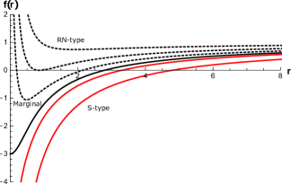
Figure 2: Different types of solutions corresponding to the metric function (22) for different values of $M$. Here $b=4$, $q=1$ and $\Lambda=0$ are used.

III.2 Second model

Considering now the metric (18) in the fields equations (15) for the Lagrangian (11) and going through the same steps as in the previous subsection, one can obtain the corresponding metric function

$$\begin{split}f(r)=&1-2bq-\frac{2M}{r}-\frac{\Lambda r^{2}}{3}-\frac{2}{3}b^{2}r^{2}+\frac{4\sqrt{b}q\sqrt{br^{2}+2q}}{3r}+\frac{2}{3}b^{3/2}r\sqrt{br^{2}+2q}\,,\end{split}$$ (28)

which behaves asymptotically as the Reissner-Nordström solution.

The solution of this black hole, as in the previous case, has one or two horizons depending on the value of the parameters $M$, $q$ and $b$. To classify the types of solutions again, we can analyze the behavior of the metric function in the limit $r\rightarrow 0$, where

$$f(r)=1-\frac{2(M-a)}{r}-2bq+\mathcal{O}(r)\,.$$ (29)

and

$$a=\frac{2}{3}\sqrt{2b}q^{3/2}\,.$$ (30)

As above we can also find the extremal mass

$$\begin{split}M_{ex}=&\frac{1}{24}\Biggr{[}bq^{2}\sqrt{(2bq+1)^{2}}+4q\sqrt{(2bq+1)^{2}}-8b^{2}q^{3}-12bq^{2}+18q+\frac{1}{b}\sqrt{(2bq+1)^{2}}-\frac{5}{b}\Biggr{]}\,.\end{split}$$ (31)

The analysis is similar if we consider the cosmological constant.

Considering the results (30) and (31), then as before we can obtain the table 2. Figure (3) illustrates the different types of solutions that can be classified for the metric function given by Eq. (28). Again the marginal case that we illustrate in this figure corresponds to a one of a regular metric function at the origin. However, it is also possible to obtain a solution belonging to the marginal case that presents a naked singularity.

Conditions		Type	Horizons
$M>a$		S	one
$M<a$	$M<M_{ex}$ $bq>1/2$	RN	zero
	$M>M_{ex}$ $bq>1/2$	RN	two
	$M=M_{ex}$ $bq>1/2$	RN	one
$M=a$	$bq>1/2$	Marginal	one
	$bq<1/2$	Marginal	zero

Table 2: Classification of the types of solutions that can be obtained from the metric function (28) as a function of the mass $M$.

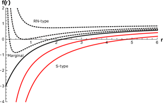
Figure 3: Different types of solutions corresponding to the metric function (28) for different values of $M$. Here $b=4$, $q=1$ and $\Lambda=0$ are used.

IV Smarr formula and first law of thermodynamics

Another characteristic of these two Born-Infeld type models is that a Smarr formula can be obtained from the first law of black hole thermodynamics. For this we must introduce a new conjugate thermodynamic quantity to each nonlinearity parameter for each model, as shown below.

In both cases we consider the cosmological constant $\Lambda$ as a thermodynamic pressure according to the relation

$$P=-\frac{\Lambda}{8\pi}\,,$$ (32)

where its thermodynamic conjugate is the volume inside the horizon $V=4\pi r_{+}^{3}/3$. Likewise, the black hole entropy is $S=\pi r_{+}^{2}$ in both cases.

IV.1 Smarr formula for the first model

From the metric function (22) we can obtain the Hawking temperature on the event horizon by using the surface gravity $\kappa$ as

$$T =\frac{\kappa}{2\pi}=\frac{1}{4\pi}\frac{df\left(r_{+}\right)}{dr}$$ (33)

$$T =\frac{-bq^{2}-b\Lambda r_{+}^{4}+br_{+}^{2}-\Lambda qr_{+}^{2}+q}{4\pi br_{+}^{3}+4\pi qr_{+}}\,.$$ (34)

To calculate the electric potential $\Phi$ on the event horizon we use the expression for the electric field given in Eq. (8)

$$\begin{split}\Phi(r_{+})=&\int_{r_{+}}^{\infty}E(r)dr=\frac{1}{8}\Bigg{[}\frac{2bqr_{+}}{br_{+}^{2}+q}-6\sqrt{bq}\tan^{-1}\Bigg{(}r_{+}+\sqrt{\frac{b}{q}}\Bigg{)}+3\pi\sqrt{bq}\Bigg{]}\,.\end{split}$$ (35)

From the metric function evaluated at the horizon, we can obtain the mass of the black hole that depends on the entropy $S$, the pressure $P$, the electric charge $q$ and the nonlinearity parameter $b$

$$\begin{split}M(S,P,q,b)=\frac{1}{12}\Bigg{[}&-6\sqrt{bq^{3}}\tan^{-1}\Bigl{(}\sqrt{\frac{bS}{\pi q}}\Bigl{)}+3\pi\sqrt{bq^{3}}+\frac{2\sqrt{S}(8PS+3)}{\sqrt{\pi}}\Bigg{]}\,.\end{split}$$ (36)

From here, we calculate the black hole temperature

$$\begin{split}T=&\left(\frac{\partial M}{\partial S}\right)_{q,P,S}\\ T=&\frac{\pi q(-bq+8PS+1)+bS(8PS+1)}{4\sqrt{\pi S}(bS+\pi q)}\,.\end{split}$$ (37)

Similarly, the electric potential on the event horizon is

$$\begin{split}\Phi\left(r_{+}\right)=&\left(\frac{\partial M}{\partial q}\right)_{S,P,b}\\ \Phi\left(r_{+}\right)=&\frac{\sqrt{bq}}{8}\Bigg{[}3\pi+\frac{2\sqrt{\pi bqS}}{bS+\pi q}-6\tan^{-1}\left(\sqrt{\frac{bS}{\pi q}}\right)\Bigg{]}\,.\end{split}$$ (38)

These last two expressions agree with those given in Eqs. (34) and (35) respectively.

We can also get the black hole volume $V$ as the conjugate quantity to pressure $P$

$$V=\left(\frac{\partial M}{\partial P}\right)_{S,q,b}\,.$$ (39)

The differentiation of the mass $M(S,P,q,b)$, leads to the first law

$$\begin{split}dM=&\left(\frac{\partial M}{\partial S}\right)_{q,P,b}dS+\left(\frac{\partial M}{\partial P}\right)_{S,q,b}dP+\\ &\left(\frac{\partial M}{\partial q}\right)_{S,P,b}dq+\left(\frac{\partial M}{\partial b}\right)_{S,q,P}db\,,\end{split}$$ (40)

where similarly to Refs. Gunasekaran:2012dq ; Yi-Huan:2010jnv and have introduced the quantity $B$ as the conjugate quantity to parameter $b$. That is,

$$\begin{split}B=&\left(\frac{\partial M}{\partial b}\right)_{S,q,P}\\ B=&\frac{q^{3/2}}{4\sqrt{b}}\left[\frac{\pi}{2}-\tan^{-1}\left(\sqrt{\frac{bS}{\pi q}}\right)-\frac{\sqrt{\pi bqS}}{bS+\pi q}\right]\,.\end{split}$$ (41)

We can obtain the corresponding Smarr formula by following the scaling arguments in Ref. Kastor:2009wy . The mass M is a homogeneous function of degree 1. If we consider that $L$ has units of length, then from the dimensional analysis we obtain the following scaling relations $S\propto L^{2}$, $P\propto L^{-2}$, $q\propto L^{1}$ and $b\propto L^{-1}$. Euler theorem allows us to obtain the following Smarr formula

$$\begin{split}M=&(2)\left(\frac{\partial M}{\partial S}\right)S+(-2)\left(\frac{\partial M}{\partial P}\right)P+(1)\left(\frac{\partial M}{\partial q}\right)q+(-1)\left(\frac{\partial M}{\partial b}\right)b\,\,\,,\end{split}$$ (42)

which we rewrite as

$$M=2TS-2VP+\Phi q-Bb\,\,\,.$$ (43)

IV.2 Smarr formula for the second model

In a similar way we can calculate the same thermodynamic quantities as above. The Hawking temperature on the event horizon $r_{+}$ is obtained using the metric function expression given by Eq. (28)

$$\begin{split}T=&\frac{\kappa}{2\pi}=\frac{1}{4\pi}\frac{df\left(r_{+}\right)}{dr}\\ T=&-\frac{1}{4\pi r_{+}}\Bigg{[}-2b^{3/2}r_{+}\sqrt{br_{+}^{2}+2q}+2b^{2}r_{+}^{2}+2bq+\Lambda r_{+}^{2}-1\Bigg{]}\,.\end{split}$$ (44)

The electric potential $\Phi$ at the event horizon is calculated with the electric field given by Eq. (13)

$$\Phi(r_{+})=\int_{r_{+}}^{\infty}E(r)dr=\sqrt{b\left(br_{+}^{2}+2q\right)}-br_{+}\,.$$ (45)

From the metric function evaluated at $r=0$, we now get

$$\begin{split}M(S,P,q,b)=&\frac{2b^{3/2}S\sqrt{bS+2\pi q}-2b^{2}S^{3/2}}{6\pi^{3/2}}+\frac{\pi\sqrt{S}(-6bq+8PS+3)}{6\pi^{3/2}}+\frac{4\pi\sqrt{b}q\sqrt{bS+2\pi q}}{6\pi^{3/2}}\,.\end{split}$$ (46)

This function allows us to calculate the following quantities. The black hole entropy as conjugate to the temperature

$$\begin{split}T=&\left(\frac{\partial M}{\partial S}\right)_{q,P,S}\\ T=&\frac{1}{4\pi^{3/2}\sqrt{S}}\Bigg{[}2b^{3/2}\sqrt{S}\sqrt{bS+2\pi q}\ -2b^{2}S-2\pi bq+8\pi PS+\pi\Bigg{]}\end{split}$$ (47)

The electric potential on the event horizon as conjugate to the electric charge $q$

$$\Phi\left(r_{+}\right)=\left(\frac{\partial M}{\partial q}\right)_{S,P,b}=\frac{\sqrt{b}\sqrt{bS+2\pi q}-b\sqrt{S}}{\sqrt{\pi}}\,.$$ (48)

Note that the same results are obtained in Eqs. (44) and (45) respectively.

Also one can get the black hole volume $V$ as the conjugate quantity to pressure $P$

$$V=\left(\frac{\partial M}{\partial P}\right)_{S,q,b}\,.$$ (49)

And the vacuum polarization $B$ as the conjugate quantity to $b$

$$\begin{split}B=&\left(\frac{\partial M}{\partial b}\right)_{S,q,P}\\ =&\frac{1}{3\pi^{3/2}\sqrt{b}}\Bigg{[}-2b^{3/2}S^{3/2}+2bS\sqrt{bS+2\pi q}-3\pi q\sqrt{bS}+\pi q\sqrt{bS+2\pi q}\Bigg{]}\end{split}$$ (50)

As above, the differentiation of the mass $M(S,P,q,b)$, leads to the first law of thermodynamics

$$dM=TdS+VdP+\Phi dq+Bdb\,,$$ (51)

and a consistent Smarr formula

$$M=2TS-2VP+\Phi q-Bb\,\,\,.$$ (52)

In Ref. Mazharimousavi:2019sgz the Smarr formula is different, a cubic term of the electrical potential appears, since the quantity $B$ was not introduced.

IV.3 Heat capacity and thermal stability of the solutions

In this subsection we discuss the thermal stability of the black hole solutions we have presented. For this purpose we calculate the heat capacity for the values of the parameters $q$, $b$ and $\Lambda$ shown in the figures. Additionally, we study the sign of the temperature where the negative sign indicates that a solution is non-physical.

The heat capacity for each of the models can be obtained with the expression (see for example Ref.  Hendi:2018sbe )

$$C_{q,P}=T\left(\frac{\partial S}{\partial T}\right)_{q,P}=T\frac{\left(\frac{\partial S}{\partial r_{+}}\right)_{q,P}}{\left(\frac{\partial T}{\partial r_{+}}\right)_{q,P}}\,\,\,.$$ (53)

For the first model, we use the temperature given by Eq. (34) and obtain

$$C_{q,P}=\frac{2\pi r_{+}^{2}\left(q+br_{+}^{2}\right)\left(bq^{2}+q\left(r_{+}^{2}\Lambda-1\right)+br_{+}^{2}\left(r_{+}^{2}\Lambda-1\right)\right)}{q^{2}-bq^{3}+2bqr_{+}^{2}-3b^{2}q^{2}r_{+}^{2}+b^{2}r_{+}^{4}+r_{+}^{2}\Lambda\left(q+br_{+}^{2}\right)^{2}}\,\,\,.$$ (54)

In the case of the second model, the temperature given by Eq. (44) allows us to obtain

$$C_{q,P}=\frac{2\pi r_{+}^{2}\sqrt{2q+br_{+}^{2}}\left(1-2bq-2b^{2}r_{+}^{2}+2r_{+}\sqrt{b^{3}\left(2q+br_{+}^{2}\right)}-r_{+}^{2}\Lambda\right)}{2b^{5/2}r_{+}^{3}+2bq\sqrt{2q+br_{+}^{2}}-2b^{2}r_{+}^{2}\sqrt{2q+br_{+}^{2}}-\sqrt{2q+br_{+}^{2}}\left(1+r_{+}^{2}\Lambda\right)}\,\,\,.$$ (55)

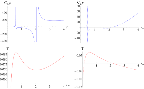
Figure 4: First model. Heat capacity $C_{q,P}$ and temperature T versus $r_{+}$ for $q=0.5$, $b=2.1$ and $\Lambda=-0.2$ (solid line) and $\Lambda=0.2$ (dashed line).

The diagrams in Fig. 4 correspond to the first model considering the values for the parameters indicated in the caption. In the AdS case (solid line diagrams) the heat capacity presents two divergent points (phase transition points), between which we have an interval of unstable solutions (i.e., $C_{q,P}<0$). If we enlarge the scale of the horizontal axis we notice that the same situation occurs for $r_{+}<0.1$. In the remaining intervals, stable solutions are found. On the other hand, the temperature is negative only for $r_{+}<0.1$. In summary, for this case we have stable physical solutions in a small interval before the first divergent point and for points from the second divergent point to infinity. In the dS case (dashed line diagrams) we find stable physical solutions only in the small interval between the single point of divergence and the point where the temperature becomes negative near the origin.

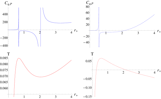
Figure 5: Second model. Heat capacity $C_{q,P}$ and temperature T versus $r_{+}$ for $q=0.5$, $b=2.1$ and $\Lambda=-0.2$ (solid line) and $\Lambda=0.2$ (dashed line).

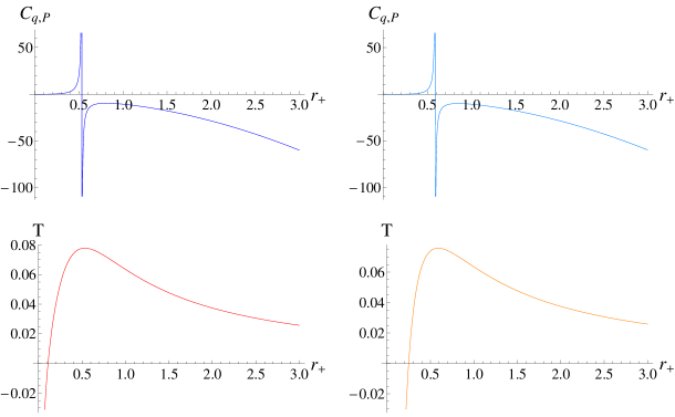
Figure 6: Heat capacity $C_{q,P}$ and temperature T versus $r_{+}$ for $q=0.5$, $b=2.1$ and $\Lambda=0$, for the first model (blue and red) and for the second model (light blue and light red).

If for the second model, we consider the same values for the parameters as for the first model, we find that the graphs behave in a similar way. The numerical differences are minimal, see the diagrams in Fig. 5. Therefore the conclusion is similar as before.

Finally, Fig. 6 illustrates the behavior of heat capacity and temperature considering $\Lambda=0$ for the two models we are analyzing. For the same choice of parameter values, we notice that the behavior is similar for both models, that is, in the small interval that is before the only point of divergence, we find stable physical solutions.

V Quasinormal spectra

This section is devoted to introduce essential ingredients to study scalar perturbations in a Born-Infeld-like background. We will focus on a massless scalar field minimally coupled to gravity for simplicity.

V.1 Wave equation for scalar perturbations

We start considering the propagation of a test real scalar field, $\Phi$, in a fixed gravitational background in a four-dimensional space-time. Considering $S[g_{\mu\nu},\Phi]$ the corresponding action, then we have the following expression

$$S[g_{\mu\nu},\Phi]\equiv\frac{1}{2}\int\mathrm{d}^{4}x\sqrt{-g}\Bigl{[}\partial^{\mu}\Phi\partial_{\mu}\Phi\Bigl{]}\,.$$ (56)

Utilizing the well-known Klein-Gordon equation (see for instance crispino ; Pappas1 ; Pappas2 ; Panotopoulos:2019gtn ; Gonzalez:2022ote ; Rincon:2020cos and references therein)

$$\frac{1}{\sqrt{-g}}\partial_{\mu}\left(\sqrt{-g}g^{\mu\nu}\partial_{\nu}\Phi\right)=0.$$ (57)

As usual, the Klein-Gordon equation may be solved applied the method of separation of variables in the appropriate coordinate system, taking into consideration the symmetries of the metric tensor. Therefore, we propose as an ansatz for the wave function the following separation of variables in spherical coordinates $r,\theta,\phi$ as follows

$$\Phi(t,r,\theta,\phi)=e^{-i\omega t}\frac{\psi(r)}{r}Y_{\ell m}(\theta,\phi),$$ (58)

where $Y_{\ell m}(\theta,\phi)$ are the usual spherical harmonics which depend on the angular coordinates only book , and $\omega$ is the unknown frequency to be determined imposing the appropriate boundary conditions.

$$\begin{split}&\frac{\omega^{2}r^{2}}{f(r)}+\frac{r}{\psi(r)}\frac{d}{dr}\left[r^{2}f(r)\frac{d}{dr}\left(\frac{\psi(r)}{r}\right)\right]+\frac{1}{Y(\Omega)}\left[\frac{1}{\sin\theta}\frac{\partial}{\partial\theta}\left(\sin\theta\frac{\partial Y(\Omega)}{\partial\theta}\right)\right]+\frac{1}{\sin^{2}\theta}\frac{1}{Y(\Omega)}\frac{\partial^{2}Y(\Omega)}{\partial\phi^{2}}=0,\end{split}$$ (59)

The angular part also satisfies

$$\begin{split}&\frac{1}{\sin\theta}\frac{\partial}{\partial\theta}\left(\sin\theta\frac{\partial Y(\Omega)}{\partial\theta}\right)+\frac{1}{\sin^{2}\theta}\frac{\partial^{2}Y(\Omega)}{\partial\phi^{2}}=-\ell(\ell+1)Y(\Omega).\end{split}$$ (60)

with $\ell(\ell+1)$ being the corresponding eigenvalue, and $\ell$ is the angular degree. The Klein-Gordon equation (Eq. (59)) is left with the radial part in the tortoise coordinate $r_{*}$:

$$\frac{\mathrm{d}^{2}\psi(r_{*})}{\mathrm{d}r_{*}^{2}}+\left[\omega^{2}-V(r_{*})\right]\psi(r_{*})=0,$$ (61)

where we have used the standard tortoise coordinate definition to transform the problem in its Schrödinger-like form, i.e.,

$$r_{*}\equiv\int\frac{\mathrm{d}r}{f(r)}\,.$$ (62)

while the effective potential barrier, $V(r)$, is computed to be

$$V(r)=f(r)\Bigg{[}\frac{\ell(\ell+1)}{r^{2}}+\frac{f^{\prime}(r)}{r}\Bigg{]},$$ (63)

and the prime denotes a derivative with respect to $r$.

Finally, the wave equation must be supplemented by the following boundary conditions

$$\Phi\rightarrow\>\exp(i\omega r_{*}),\;\;\;\;\;\;r_{*}\rightarrow-\infty$$ (64)

$$\Phi\rightarrow\>\exp(-i\omega r_{*}),\;\;\;\;\;\;r_{*}\rightarrow\infty$$ (65)

Given the time dependence of the scalar wave function, $\Phi\sim\exp(-i\omega t)$, a frequency with a negative imaginary part implies a decaying (stable) mode, whereas a frequency with a positive imaginary part implies an increasing (unstable) mode.

In Fig. 7, we show the effective potential for the two models discussed in this manuscript. In particular, the first row corresponds to the first model, and the second row to the second model. The qualitative behavior of the effective potential for both cases is essentially the same for the numerical values used.

The first column corresponds to the effective potential for the first model (top) and the second model (bottom) when the angular degree $\ell$ varies. Thus, we observe that when we increase the angular number $\ell$, the effective potential increases too. Similarly, when $\ell$ increases, $r_{\text{max}}$ is slightly shifted to the right (in both cases).

The second column corresponds to the effective potential for the first model (top) and the second model (bottom) when the non-linear parameter $b$ varies. Similarly to the previous situation, we observe that when we increase the parameter $b$, the effective potential increases too, but now, the difference in intensity is soft. Finally, when $b$ increases, $r_{\text{max}}$ is slightly shifted to the left (in both cases).

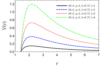
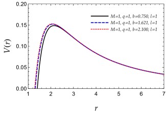
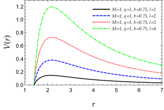
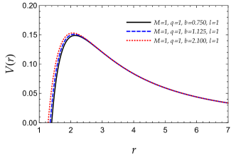
Figure 7: Effective potential barrier for scalar perturbations against the radial coordinate for the parameters shown in the panels. The first row corresponds to the first model, whereas the second row shows the behavior of the potencial corresponding to the second model. In all four panels we have assumed $\Lambda=0$.

V.2 Numerical computation: WKB method

Obtaining exact analytic expressions for the quasinormal spectra of black holes is possible only in a few number of cases, for instance: i) when the effective potential barrier acquires the form of the Pöschl-Teller potential potential ; ferrari ; cardoso2 ; lemos ; molina ; panotop1 , or ii) when the corresponding differential equation (for the radial part of the wave function) can be recast into the Gauss’ hypergeometric function exact1 ; exact2 ; exact3 ; Gonzalez:2010vv ; exact4 ; exact5 ; exact6 .

In general, it is not possible to obtain an exact analytic solution due to the complexity and non-trivial structure of the differential equation involved. This is the reason why it is necessary to employ one of the numerical schemes available in the literature.

Up to now there a variety of methods used to obtain, in a very good accuracy, the QN spectra of black holes. One can mention for example the Frobenius method, the generalization of the Frobenius series, fit and interpolation approach, the method of continued fraction, although more methods are known to exist. For more details the interested reader may consult for instance review3 , and for recent works Singh:2022ycn ; Nomura:2021efi ; Sakalli:2022xrb and references therein.

Given that the WKB semi-classical approximation wkb0 ; wkb1 ; wkb2 ; wkb3 ; wkb4 is well-known, we shall avoid the inclusion of unnecessary details. Adopting the WKB method, the QN spectra may be computed via the following expression

$$\omega_{n}^{2}=V_{0}+(-2V_{0}^{\prime\prime})^{1/2}\Lambda(n)-i\nu(-2V_{0}^{\prime\prime})^{1/2}[1+\Omega(n)]\,,$$ (66)

where i) $V_{0}^{\prime\prime}$ is the second derivative of the potential evaluated at the maximum, ii) $\nu=n+1/2$, $V_{0}$ is the maximum of the effective potential barrier, iii) $n=0,1,2...$ is the overtone number, while the functions $\Lambda(n),\Omega(n)$ are long and complicated expressions of $\nu$ (and derivatives of the potential evaluated at the maximum), and they can be found for instance in wkb3 .

At this point it should be mentioned that the 3rd order approximation was first constructed by Iyer and Will in wkb1 , and it was subsequently extended to higher orders. Thus, to perform our computations, we have used here a Wolfram Mathematica wolfram notebook utilizing the WKB method at any order from one to six code .

In the present work we have adopted the WKB method at sixth order. Besides, it should be mentioned that for a given angular degree, $\ell$, we have considered values $n<\ell$ only, since it is known that the method works well for high angular degrees. For higher order WKB corrections (and recipes for simple, quick, efficient and accurate computations) see Opala ; Konoplya:2019hlu ; RefExtra2 . In particular, we should mention that as the WKB series converges only asymptotically, there is no mathematically strict criterium for evaluation of an error according to Konoplya:2019hlu . However, the sixth/seventh order usually produce the best results. In that direction, taking into account the Padé approximations we can have a higher accuracy of the WKB approach. This analysis, however, will be performed in a future study.

Table 3: Quasinormal frequencies (varying $\ell$ and $n$) for the two models and the three behaviors (S-type, RN-type and Marginal) considered in this work. The numerical values of the parameters $M,q,b$ assumed to obtain the QNMs are the ones shown in Fig. 7.

	QN frequencies for Scalar perturbations
	First model	Second model
Type S $(\ell=2)$	$\omega(n=0)$ = 0.605941 - 0.101944 I	$\omega(n=0)$ = 0.621496 - 0.0990191 I
	$\omega(n=1)$ = 0.592259 - 0.309586 I	$\omega(n=1)$ = 0.749904 - 0.2436500 I
Type RN $(\ell=2)$	$\omega(n=0)$ = 0.618099 - 0.096235 I	$\omega(n=0)$ = 2763.360 + 0.2359470 I
	$\omega(n=1)$ = 0.605848 - 0.291446 I	$\omega(n=1)$ = 9962.160 + 0.7206980 I
Type RN $(\ell=12)$	$\omega(n=0)$ = 3.07474 - 0.0958944 I	$\omega(n=0)$ = 40.4016 - 0.00272247 I
	$\omega(n=1)$ = 3.07214 - 0.2877990 I	$\omega(n=1)$ = 145.237 + 0.00786804 I
Type RN $(\ell=20)$	$\omega(n=0)$ = 5.04189 - 0.095885 I	$\omega(n=0)$ = 0.077788 - 5.42437 I
	$\omega(n=1)$ = 5.04030 - 0.287699 I	$\omega(n=1)$ = 0.029747 - 26.2024 I
	$\omega(n=2)$ = 5.03713 - 0.479642 I	$\omega(n=2)$ = 0.019038 + 68.0079 I
Type M $(\ell=2)$	$\omega(n=0)$ = 0.615788 - 0.097606 I	$\omega(n=0)$ = 0.937076 - 0.0634837 I
	$\omega(n=1)$ = 0.599094 - 0.302352 I	$\omega(n=1)$ = 2.594380 - 0.0642422 I

Our findings may be summarized as follows: Regarding the sign of the imaginary part of the frequencies, in the first model all frequencies are characterized by negative imaginary part, whereas in the second model, the same holds for S-type and Marginal behaviour. In contrary, in the RN-type behaviour, for $\ell=2$ both modes are characterized by a positive imaginary part, and then considering higher values of the angular degree, after a certain value of the overtone, $n$, the imaginary part changes sign.

Regarding the impact of $n,\ell$ on the spectra, a direct comparison between the two models reveals the following features: a) Regarding the S-type behaviour, the imaginary part becomes more negative with $n$ in both models, while the real part decreases with $n$ in the first model and increases with $n$ in the second model. b) Regarding the Marginal behaviour, just like in the previous case, the imaginary part becomes more negative with $n$, although only slightly in the second model, while the real part decreases with $n$ in the first model and increases with $n$ in the second model. Finally, in the RN-type behaviour, the real part of the frequencies increases with $\ell$ in the first model, and decreases with $\ell$ in the second model.

Before we conclude, and as far as future work is concerned, we add here as a final comment that it would be interesting to investigate even further the properties of the novel black hole solutions discussed in the present article. In particular, it would be worth studying the QN spectra for Dirac and Maxwell fields, and also the deflection of light as well as their shadow casts cunha . We hope to be able to address some of those exciting topics in forthcoming publications.

VI Conclusions

In the present paper, we investigated in detail two novel electrically charged black hole solutions within non-linear electrodynamics of Born-Infeld type in four-dimensional space-time. In particular, we computed the metric function for each Lagrangian density considered here, and we demonstrated that each solution exhibits three distinct behaviours (S-type, RN-type and Marginal) depending on the numerical values of the parameters. Next, we discussed black hole thermodynamics for both models as well as the Smarr formula, which was shown to be compatible with the first law of black hole mechanics. We extended the usual Smarr formula defining a new conjugate thermodynamic quantity associated to the non-linear parameter, $b$. Finally, we computed the frequencies of some quasinormal modes for scalar perturbations analyzing the propagation of a massless, canonical scalar field varying the parameters $\{b,\ell,n\}$ for certain values of $M,q$. The WKB method of sixth order was employed to compute the modes numerically. We found that as far as the first model is concerned, the frequencies are always characterized by a negative imaginary part, irrespectively of the type of behaviour. Regarding the second model, however, our numerical results show that in the S-type and marginal type, the frequencies are characterized by a negative imaginary part, but in the RN-type some frequencies are characterized by a positive imaginary part. In summary, naively one might expect to see almost identical spectra. Our findings, however, show that although the models look very similar, their quasinormal spectra are characterized by certain differences.

Data Availability Statement

Authors’ comment: This is a theoretical study, and for that reason no experimental data are presented.

References

- (1) W. Heisenberg and H. Euler, “Folgerungen aus der Diracschen Theorie des Positrons,” Z. Phys. 98 (1936) 714 [physics/0605038].
- (2) M. Born and L. Infeld, “Foundations of the new field theory,” Proc. Roy. Soc. Lond. A 144, no. 852, 425 (1934).
- (3) H. H. Soleng, “Charged black points in general relativity coupled to the logarithmic U(1) gauge theory,” Phys. Rev. D 52, 6178-6181 (1995). [arXiv:hep-th/9509033 [hep-th]].
- (4) S. I. Kruglov, “A model of nonlinear electrodynamics,” Annals Phys. 353, 299-306 (2014).
- (5) S. I. Kruglov, “Acceleration of Universe by Nonlinear Electromagnetic Fields,” Int. J. Mod. Phys. D 25, no.11, 1640002 (2016).
- (6) S. I. Kruglov, “Magnetized black holes and nonlinear electrodynamics,” Int. J. Mod. Phys. A 32, no.23n24, 1750147 (2017).
- (7) S. I. Kruglov, “Nonlinear Electrodynamics and Magnetic Black Holes,” Annalen Phys. 529, no.8, 1700073 (2017).
- (8) P. Gaete and J. A. Helayël-Neto, “A note on nonlinear electrodynamics,” EPL 119, no.5, 51001 (2017).
- (9) P. Gaete, J. A. Helayël-Neto and L. P. R. Ospedal, “Coulomb’s law modification driven by a logarithmic electrodynamics,” EPL 125, no.5, 51001 (2019).
- (10) S. H. Mazharimousavi and M. Halilsoy, “Electric Black Holes in a Model of Nonlinear Electrodynamics,” Annalen Phys. 531, no.12, 1900236 (2019).
- (11) S. H. Mazharimousavi and M. Halilsoy, “Electric and magnetic black holes in a new nonlinear electrodynamics model,” Annals Phys. 433, 168579 (2021).
- (12) I. Gullu and S. H. Mazharimousavi, “Double-logarithmic nonlinear electrodynamics,” Phys. Scripta 96, no.4, 045217 (2021).
- (13) I. Bandos, K. Lechner, D. Sorokin and P. K. Townsend, “A non-linear duality-invariant conformal extension of Maxwell’s equations,” Phys. Rev. D 102, 121703 (2020).
- (14) S. I. Kruglov, “On generalized ModMax model of nonlinear electrodynamics,” Phys. Lett. B 822, 136633 (2021).
- (15) S. Belmar-Herrera and L. Balart, “Charged black holes from a family of Born-Infeld-type electrodynamics models,” [arXiv:2211.14412 [gr-qc]].
- (16) H. Reissner, Annalen Phys. 355 (1916) 106-120.
- (17) M. Aiello, R. Ferraro and G. Giribet, Phys. Rev. D 70 (2004), 104014 [arXiv:gr-qc/0408078 [gr-qc]].
- (18) T. K. Dey, Phys. Lett. B 595 (2004), 484-490 [arXiv:hep-th/0406169 [hep-th]].
- (19) S. Kanzi, S. H. Mazharimousavi and İ. Sakallı, Annals Phys. 422 (2020), 168301 [arXiv:2007.05814 [hep-th]].
- (20) K. Jafarzade, M. Kord Zangeneh and F. S. N. Lobo, JCAP 04 (2021), 008 [arXiv:2010.05755 [gr-qc]].
- (21) B. Pourhassan, M. Dehghani, S. Upadhyay, I. Sakalli and D. V. Singh, Mod. Phys. Lett. A 37 (2022) no.33n34, 2250230 [arXiv:2301.01603 [gr-qc]].
- (22) H. P. de Oliveira, Class. Quant. Grav. 11 (1994), 1469-1482
- (23) W. Javed, M. Atique, R. C. Pantig and A. Övgün, Int. J. Geom. Meth. Mod. Phys. 20 (2023) no.03, 2350040
- (24) Y. Kumaran and A. Övgün, Symmetry 14 (2022) no.10, 2054 [arXiv:2210.00468 [gr-qc]].
- (25) M. Okyay and A. Övgün, JCAP 01 (2022) no.01, 009 [arXiv:2108.07766 [gr-qc]].
- (26) W. Javed, J. Abbas and A. Övgün, Eur. Phys. J. C 79 (2019) no.8, 694 [arXiv:1908.09632 [physics.gen-ph]].
- (27) O. Gurtug, S. H. Mazharimousavi and M. Halilsoy, “2+1-dimensional electrically charged black holes in Einstein - power Maxwell Theory,” Phys. Rev. D 85 (2012) 104004 [arXiv:1010.2340 [gr-qc]].
- (28) S. H. Mazharimousavi, O. Gurtug, M. Halilsoy and O. Unver, “2+1 dimensional magnetically charged solutions in Einstein-Power-Maxwell theory,” Phys. Rev. D 84, 124021 (2011) [arXiv:1103.5646 [gr-qc]].
- (29) W. Xu and D. C. Zou, “ -Dimensional charged black holes with scalar hair in Einstein–Power–Maxwell Theory,” Gen. Rel. Grav. 49, no. 6, 73 (2017) [arXiv:1408.1998 [hep-th]].
- (30) Á. Rincón, E. Contreras, P. Bargueño, B. Koch, G. Panotopoulos and A. Hernández-Arboleda, “Scale dependent three-dimensional charged black holes in linear and non-linear electrodynamics,” Eur. Phys. J. C 77, no. 7, 494 (2017) [arXiv:1704.04845 [hep-th]].
- (31) G. Panotopoulos and Á. Rincón, “Quasinormal modes of black holes in Einstein-power-Maxwell theory,” Int. J. Mod. Phys. D 27 (2017) no.03, 1850034 [arXiv:1711.04146 [hep-th]].
- (32) Á. Rincón and G. Panotopoulos, “Quasinormal modes of scale dependent black holes in ( 1+2 )-dimensional Einstein-power-Maxwell theory,” Phys. Rev. D 97 (2018) no.2, 024027 [arXiv:1801.03248 [hep-th]].
- (33) G. Panotopoulos and Á. Rincón, “Greybody factors for a minimally coupled scalar field in three-dimensional Einstein-power-Maxwell black hole background,” Phys. Rev. D 97 (2018) no.8, 085014 [arXiv:1804.04684 [hep-th]].
- (34) Á. Rincón, E. Contreras, P. Bargueño, B. Koch and G. Panotopoulos, “Scale-dependent ( )-dimensional electrically charged black holes in Einstein-power-Maxwell theory,” Eur. Phys. J. C 78 (2018) no.8, 641 [arXiv:1807.08047 [hep-th]].
- (35) G. Panotopoulos and Á. Rincón, “Charged slowly rotating toroidal black holes in the (1 + 3)-dimensional Einstein-power-Maxwell theory,” Int. J. Mod. Phys. D 28 (2018) no.01, 1950016 [arXiv:1808.05171 [gr-qc]].
- (36) G. Panotopoulos, “Charged scalar fields around Einstein-power-Maxwell black holes,” Gen. Rel. Grav. 51 (2019) no.6, 76.
- (37) G. Panotopoulos, “Quasinormal modes of charged black holes in higher-dimensional Einstein-power-Maxwell theory,” Axioms 9 (2020) no.1, 33 [arXiv:2005.08338 [gr-qc]].
- (38) M. Hassaine and C. Martinez, “Higher-dimensional charged black holes solutions with a nonlinear electrodynamics source,” Class. Quant. Grav. 25, 195023 (2008). [arXiv:0803.2946 [hep-th]].
- (39) H. A. Gonzalez, M. Hassaine and C. Martinez, “Thermodynamics of charged black holes with a nonlinear electrodynamics source,” Phys. Rev. D 80, 104008 (2009). [arXiv:0909.1365 [hep-th]].
- (40) J. Bardeen, presented at GR5, Tiflis, U.S.S.R., and published in the conference proceedings in the U.S.S.R. (1968)
- (41) A. Borde, “Regular black holes and topology change,” Phys. Rev. D 55 (1997) 7615 [gr-qc/9612057].
- (42) E. Ayon-Beato and A. Garcia, “Regular black hole in general relativity coupled to nonlinear electrodynamics,” Phys. Rev. Lett. 80 (1998) 5056 [gr-qc/9911046].
- (43) E. Ayon-Beato and A. Garcia, “Nonsingular charged black hole solution for nonlinear source,” Gen. Rel. Grav. 31 (1999) 629 [gr-qc/9911084].
- (44) E. Ayon-Beato and A. Garcia, “New regular black hole solution from nonlinear electrodynamics,” Phys. Lett. B 464 (1999) 25 [hep-th/9911174].
- (45) K. A. Bronnikov, “Regular magnetic black holes and monopoles from nonlinear electrodynamics,” Phys. Rev. D 63 (2001) 044005 [gr-qc/0006014].
- (46) I. Dymnikova, “Regular electrically charged structures in nonlinear electrodynamics coupled to general relativity,” Class. Quant. Grav. 21 (2004) 4417 [gr-qc/0407072].
- (47) S. A. Hayward, “Formation and evaporation of regular black holes,” Phys. Rev. Lett. 96 (2006) 031103 [gr-qc/0506126].
- (48) L. Balart and E. C. Vagenas, “Regular black hole metrics and the weak energy condition,” Phys. Lett. B 730 (2014) 14 [arXiv:1401.2136 [gr-qc]].
- (49) L. Balart and E. C. Vagenas, “Regular black holes with a nonlinear electrodynamics source,” Phys. Rev. D 90 (2014) no.12, 124045 [arXiv:1408.0306 [gr-qc]].
- (50) M. E. Rodrigues, E. L. B. Junior and M. V. de Sousa Silva, “Using dominant and weak energy conditions for build new classe of regular black holes,” JCAP 02, 059 (2018).
- (51) A. Einstein, “The Foundation of the General Theory of Relativity,” Annalen Phys. 49, no.7, 769-822 (1916).
- (52) K. Akiyama et al. [Event Horizon Telescope], “First M87 Event Horizon Telescope Results. I. The Shadow of the Supermassive Black Hole,” Astrophys. J. Lett. 875, L1 (2019) [arXiv:1906.11238 [astro-ph.GA]].
- (53) B. P. Abbott et al. [LIGO Scientific and Virgo], “Observation of Gravitational Waves from a Binary Black Hole Merger,” Phys. Rev. Lett. 116, no.6, 061102 (2016) [arXiv:1602.03837 [gr-qc]].
- (54) J. M. Bardeen, B. Carter and S. W. Hawking, “The Four laws of black hole mechanics,” Commun. Math. Phys. 31, 161-170 (1973).
- (55) S. W. Hawking, “Black hole explosions,” Nature 248, 30-31 (1974).
- (56) S. W. Hawking, “Particle Creation by Black Holes,” Commun. Math. Phys. 43, 199-220 (1975) [erratum: Commun. Math. Phys. 46, 206 (1976)].
- (57) J. D. Bekenstein, “Black holes and entropy,” Phys. Rev. D 7, 2333-2346 (1973).
- (58) L. Smarr, “Mass formula for Kerr black holes,” Phys. Rev. Lett. 30, 71-73 (1973) [erratum: Phys. Rev. Lett. 30, 521-521 (1973)].
- (59) L. Balart and S. Fernando, “A Smarr formula for charged black holes in nonlinear electrodynamics,” Mod. Phys. Lett. A 32, no.39, 1750219 (2017). [arXiv:1710.07751 [gr-qc]].
- (60) M. S. Ma and R. Zhao, “Corrected form of the first law of thermodynamics for regular black holes,” Class. Quant. Grav. 31, 245014 (2014). [arXiv:1411.0833 [gr-qc]].
- (61) T. Regge and J. A. Wheeler, “Stability of a Schwarzschild singularity,” Phys. Rev. 108, 1063-1069 (1957).
- (62) F. J. Zerilli, “Effective potential for even parity Regge-Wheeler gravitational perturbation equations,” Phys. Rev. Lett. 24, 737-738 (1970).
- (63) F. J. Zerilli, “Gravitational field of a particle falling in a schwarzschild geometry analyzed in tensor harmonics,” Phys. Rev. D 2, 2141-2160 (1970).
- (64) F. J. Zerilli, “Perturbation analysis for gravitational and electromagnetic radiation in a reissner-nordstroem geometry,” Phys. Rev. D 9, 860-868 (1974).
- (65) V. Moncrief, “Gauge-invariant perturbations of Reissner-Nordstrom black holes,” Phys. Rev. D 12, 1526-1537 (1975).
- (66) S. A. Teukolsky, “Rotating black holes - separable wave equations for gravitational and electromagnetic perturbations,” Phys. Rev. Lett. 29, 1114-1118 (1972).
- (67) S. Chandrasekhar, “The mathematical theory of black holes,” OXFORD, UK: CLARENDON (1985) 646 P.
- (68) S. Fernando and D. Krug, “Charged black hole solutions in Einstein-Born-Infeld gravity with a cosmological constant,” Gen. Rel. Grav. 35, 129-137 (2003). [arXiv:hep-th/0306120 [hep-th]].
- (69) S. Fernando, “Thermodynamics of Born-Infeld-anti-de Sitter black holes in the grand canonical ensemble,” Phys. Rev. D 74, 104032 (2006). [arXiv:hep-th/0608040 [hep-th]].
- (70) S. Gunasekaran, R. B. Mann and D. Kubiznak, “Extended phase space thermodynamics for charged and rotating black holes and Born-Infeld vacuum polarization,” JHEP 11, 110 (2012). [arXiv:1208.6251 [hep-th]].
- (71) N. Bretón, T. Clark and S. Fernando, “Quasinormal modes and absorption cross-sections of Born–Infeld–de Sitter black holes,” Int. J. Mod. Phys. D 26, no.10, 1750112 (2017). [arXiv:1703.10070 [gr-qc]].
- (72) W. Yi-Huan, “Energy and first law of thermodynamics for Born-Infeld-anti-de-Sitter black hole,” Chin. Phys. B 19, 090404 (2010).
- (73) D. Kastor, S. Ray and J. Traschen, Enthalpy and the Mechanics of AdS Black Holes, Class. Quant. Grav. 26, 195011 (2009).
- (74) S. H. Hendi and M. Momennia, “AdS charged black holes in Einstein–Yang–Mills gravity’s rainbow: Thermal stability and criticality,” Phys. Lett. B 777, 222-234 (2018).
- (75) L. C. B. Crispino, A. Higuchi, E. S. Oliveira and J. V. Rocha, “Greybody factors for nonminimally coupled scalar fields in Schwarzschild–de Sitter spacetime,” Phys. Rev. D 87 (2013) 104034 [arXiv:1304.0467 [gr-qc]].
- (76) P. Kanti, T. Pappas and N. Pappas, “Greybody factors for scalar fields emitted by a higher-dimensional Schwarzschild–de Sitter black hole,” Phys. Rev. D 90 (2014) no.12, 124077 [arXiv:1409.8664 [hep-th]].
- (77) T. Pappas, P. Kanti and N. Pappas, “Hawking radiation spectra for scalar fields by a higher-dimensional Schwarzschild–de Sitter black hole,” Phys. Rev. D 94 (2016) no.2, 024035 [arXiv:1604.08617 [hep-th]].
- (78) G. Panotopoulos and Á. Rincón, “Quasinormal modes of five-dimensional black holes in non-commutative geometry,” Eur. Phys. J. Plus 135 (2020) no.1, 33 [arXiv:1910.08538 [gr-qc]].
- (79) P. A. González, E. Papantonopoulos, Á. Rincón and Y. Vásquez, Phys. Rev. D 106 (2022) no.2, 024050 [arXiv:2205.06079 [gr-qc]].
- (80) Á. Rincón and V. Santos, Eur. Phys. J. C 80 (2020) no.10, 910 [arXiv:2009.04386 [gr-qc]].
- (81) C. Muller, in Lecture Notes in Mathematics: Spherical Harmonics (Springer-Verlag, Berlin-Heidelberg, 1966).
- (82) G. Poschl and E. Teller, “Bemerkungen zur Quantenmechanik des anharmonischen Oszillators,” Z. Phys. 83 (1933) 143.
- (83) V. Ferrari and B. Mashhoon, “New approach to the quasinormal modes of a black hole,” Phys. Rev. D 30 (1984) 295.
- (84) V. Cardoso and J. P. S. Lemos, “Scalar, electromagnetic and Weyl perturbations of BTZ black holes: Quasinormal modes,” Phys. Rev. D 63 (2001) 124015 [gr-qc/0101052].
- (85) V. Cardoso and J. P. S. Lemos, “Quasinormal modes of the near extremal Schwarzschild-de Sitter black hole,” Phys. Rev. D 67 (2003) 084020 doi:10.1103/PhysRevD.67.084020 [gr-qc/0301078].
- (86) C. Molina, “Quasinormal modes of d-dimensional spherical black holes with near extreme cosmological constant,” Phys. Rev. D 68 (2003) 064007 [gr-qc/0304053].
- (87) G. Panotopoulos, “Electromagnetic quasinormal modes of the nearly-extremal higher-dimensional Schwarzschild–de Sitter black hole,” Mod. Phys. Lett. A 33 (2018) no.23, 1850130 [arXiv:1807.03278 [gr-qc]].
- (88) D. Birmingham, “Choptuik scaling and quasinormal modes in the AdS / CFT correspondence,” Phys. Rev. D 64 (2001) 064024 [arXiv:[hep-th/0101194]].
- (89) S. Fernando, “Quasinormal modes of charged dilaton black holes in (2+1)-dimensions,” Gen. Rel. Grav. 36 (2004) 71 [arXiv:[hep-th/0306214]].
- (90) S. Fernando, “Quasinormal modes of charged scalars around dilaton black holes in 2+1 dimensions: Exact frequencies,” Phys. Rev. D 77 (2008) 124005 [arXiv:0802.3321 [hep-th]].
- (91) P. Gonzalez, E. Papantonopoulos and J. Saavedra, “Chern-Simons black holes: scalar perturbations, mass and area spectrum and greybody factors,” JHEP 08 (2010), 050 [arXiv:1003.1381 [hep-th]].
- (92) K. Destounis, G. Panotopoulos and Á. Rincón, “Stability under scalar perturbations and quasinormal modes of 4D Einstein–Born–Infeld dilaton spacetime: exact spectrum,” Eur. Phys. J. C 78 (2018) no.2, 139 [arXiv:1801.08955 [gr-qc]].
- (93) A. Ovgün and K. Jusufi, “Quasinormal Modes and Greybody Factors of gravity minimally coupled to a cloud of strings in Dimensions,” Annals Phys. 395, 138 (2018) [arXiv:1801.02555 [gr-qc]].
- (94) Á. Rincón and G. Panotopoulos, “Greybody factors and quasinormal modes for a nonminimally coupled scalar field in a cloud of strings in (2+1)-dimensional background,” Eur. Phys. J. C 78, no. 10, 858 (2018) [arXiv:1810.08822 [gr-qc]].
- (95) R. A. Konoplya and A. Zhidenko, “Quasinormal modes of black holes: From astrophysics to string theory,” Rev. Mod. Phys. 83 (2011) 793 [arXiv:1102.4014 [gr-qc]].
- (96) D. V. Singh, A. Shukla and S. Upadhyay, “Quasinormal modes, shadow and thermodynamics of black holes coupled with nonlinear electrodynamics and cloud of strings,” Annals Phys. 447 (2022), 169157 [arXiv:2211.09673 [gr-qc]].
- (97) K. Nomura and D. Yoshida, “Quasinormal modes of charged black holes with corrections from nonlinear electrodynamics,” Phys. Rev. D 105 (2022) no.4, 044006 [arXiv:2111.06273 [gr-qc]].
- (98) İ. Sakalli and S. Kanzi, “Topical Review: greybody factors and quasinormal modes for black holes in various theories - fingerprints of invisibles,” Turk. J. Phys. 46 (2022) no.2, 51-103 [arXiv:2205.01771 [hep-th]].
- (99) B. F. Schutz and C. M. Will, “Black Hole Normal Modes: A Semianalytic Approach,” Astrophys. J. 291 (1985) L33.
- (100) S. Iyer and C. M. Will, “Black Hole Normal Modes: A WKB Approach. 1. Foundations and Application of a Higher Order WKB Analysis of Potential Barrier Scattering,” Phys. Rev. D 35 (1987) 3621.
- (101) S. Iyer, “Black Hole Normal Modes: A Wkb Approach. 2. Schwarzschild Black Holes,” Phys. Rev. D 35 (1987) 3632.
- (102) K. D. Kokkotas and B. F. Schutz, “Black Hole Normal Modes: A WKB Approach. 3. The Reissner-Nordstrom Black Hole,” Phys. Rev. D 37 (1988) 3378.
- (103) E. Seidel and S. Iyer, “Black Hole Normal Modes: A Wkb Approach. 4. Kerr Black Holes,” Phys. Rev. D 41 (1990) 374.
- (104) http://www.wolfram.com
- (105) R. A. Konoplya and A. Zhidenko, “Passage of radiation through wormholes of arbitrary shape,” Phys. Rev. D 81 (2010) 124036 [arXiv:1004.1284 [hep-th]].
- (106) J. Matyjasek and M. Opala, “Quasinormal modes of black holes. The improved semianalytic approach,” Phys. Rev. D 96 (2017) no.2, 024011 [arXiv:1704.00361 [gr-qc]].
- (107) R. A. Konoplya, A. Zhidenko and A. F. Zinhailo, “Higher order WKB formula for quasinormal modes and grey-body factors: recipes for quick and accurate calculations,” Class. Quant. Grav. 36 (2019) 155002 [arXiv:1904.10333 [gr-qc]].
- (108) Y. Hatsuda, “Quasinormal modes of black holes and Borel summation,” arXiv:1906.07232 [gr-qc].
- (109) P. V. P. Cunha and C. A. R. Herdeiro, “Shadows and strong gravitational lensing: a brief review,” Gen. Rel. Grav. 50, no.4, 42 (2018) [arXiv:1801.00860 [gr-qc]].