Reference-guided Controllable Inpainting of Neural Radiance Fields
Abstract
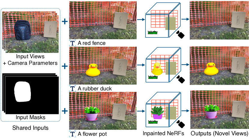
The popularity of Neural Radiance Fields (NeRFs) for view synthesis has led to a desire for NeRF editing tools. Here, we focus on inpainting regions in a view-consistent and controllable manner. In addition to the typical NeRF inputs and masks delineating the unwanted region in each view, we require only a single inpainted view of the scene, i.e., a reference view. We use monocular depth estimators to back-project the inpainted view to the correct 3D positions. Then, via a novel rendering technique, a bilateral solver can construct view-dependent effects in non-reference views, making the inpainted region appear consistent from any view. For non-reference disoccluded regions, which cannot be supervised by the single reference view, we devise a method based on image inpainters to guide both the geometry and appearance. Our approach shows superior performance to NeRF inpainting baselines, with the additional advantage that a user can control the generated scene via a single inpainted image. Please visit our project page. ††footnotetext: ∗ Authors contributed equally.
1 Introduction
There has long been intense interest in manipulating images, due to the broad range of content creation use cases. Object removal and insertion, corresponding to the image inpainting task, is among the most studied manipulations. Current inpainting models are capable of generating perceptually realistic content that conforms to the surrounding image. Yet, these models are limited to single 2D image inputs; our goal is to continue progress in applying such models to the manipulation of full 3D scenes.
The advent of Neural Radiance Fields (NeRFs) has made transforming real 2D photos into realistic 3D representations more accessible. As algorithmic improvements continue and computational requirements lessen, such 3D representations may become ubiquitous. We are thus interested in enabling the same manipulations of 3D NeRFs that are available for images, particularly inpainting (see Fig. 1).
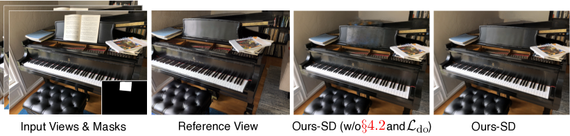
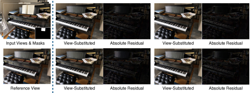
Inpainting in 3D is non-trivial for a number of reasons, such as the paucity of 3D data and the need to account for 3D geometry as well as appearance. Using NeRFs as a scene representation comes with additional challenges. First, the “black box” nature of implicit neural representations makes it infeasible to simply edit the underlying data structure based on geometric understanding. Second, because NeRFs are trained from images, special considerations are required for maintaining multiview consistency. Simply independently inpainting the constituent images using powerful 2D inpainters yields viewpoint-inconsistent imagery (see Fig. 2), leading to visually unrealistic outputs.
One approach is to attempt to resolve these inconsistencies post hoc. For example, NeRF-In [34] simply combines views via a pixelwise loss. More recently, SPIn-NeRF [42] improved on this strategy by employing a perceptual loss [84] instead. Yet, this fails when the inpainted views are perceptually different (i.e., the textures are far apart, even in the perceptual metric space). This limits applicability in the case of complex appearances or novel object insertion. For instance, recent diffusion-based inpainters (e.g., [55, 76]) can controllably hallucinate novel objects in 2D inpaintings – utilizing this capability is currently impossible in the post hoc framework. In addition, this approach impedes the preservation of specific desired details (i.e., inter-image conflicts prevent conservation of exact textures).
In contrast, others have considered single-reference inpainting (e.g., [34]): using only one inpainted view precludes inconsistencies by construction. However, this lack of 3D information introduces a different set of challenges, including (a) poor visual quality in views far from the reference, in part due to a lack of geometric supervision, (b) lack of view-dependent effects (VDEs), and (c) disocclusions.
In this work, we utilize a single inpainted reference, thus immediately avoiding view inconsistencies, and present a novel algorithm for handling challenges (a-c). First, to geometrically supervise the inpainted area, we utilize an optimization-based formulation with monocular depth estimation. Second, we show how to simulate VDEs of non-reference views from the reference viewpoint. This enables a guided inpainting approach, propagating non-reference colours (with VDEs) into the mask. Finally, we inpaint disoccluded appearance and geometry in a consistent manner.
We enumerate our contributions as follows: (i) a single-reference 3D inpainting algorithm (depicted in Fig. 1), which avoids visual quality deterioration at views far from the reference; (ii) a unified method for constructing supervision for masked and disoccluded areas; (iii) a novel approach to generating VDEs in non-reference views, without multiview appearance information; (iv) significant empirical improvements over prior work, not only in the unprecedented sharpness of novel inpainted views, but also in terms of controllability, enabling users to insert novel objects into 3D scenes by simply providing a single inpainted 2D view.
2 Related Work
Image Inpainting. Inpainting 2D images has a long research history [21, 9, 13, 5, 64]. Neural models represent the state of the art, with advances in perceptual plausibility [61, 29, 20], multi-scale processing [18, 82, 73], novel architectures [77, 29, 33, 75], and generative modelling (e.g., adversarial [47, 85] or denoising diffusion [55, 36, 56, 45, 37]). To address the ill-posed nature of the inpainting problem, pluralistic inpainting methods construct multiple plausible outputs [85, 87, 55, 71]. Yet, all these methods are 3D unaware. In contrast, 3D-aware works are only partially 3D [79], limited to simple foreground/background scenarios [59, 22], or cannot synthesize novel views of the inpainted result [86, 88]. In contrast, we inpaint in an inherently 3D manner via NeRFs, allowing novel-view synthesis of the inpainted scene.
NeRF Editing. Neural rendering [65] has received significant attention following the success of NeRFs [41], which combines differentiable volumetric rendering [15, 67] and positional encodings [12, 68, 62]. Rapid NeRF developments have improved visual quality [11, 2, 3, 32, 69], fitting or inference speed [58, 6, 44, 80, 8, 14, 53, 27], and data requirements [81, 72, 31, 74, 49, 19]. As NeRFs become more accessible, editing them in 3D has become a topic of interest. Recent works provide 3D scene editing capabilities [26, 43, 70, 78, 83, 35, 24, 28, 60, 10, 23, 30], but either focus on non-inpainting tasks, consider different data availability scenarios, or are limited to simple objects. The first NeRF inpainting works are NeRF-In [34] and SPIn-NeRF [42]. Both methods use 2D image inpainters as priors, and fill the unwanted regions of both the training views and the rendered training depths, to guide the generation of the inpainted NeRF. While NeRF-In [34] does not systematically consider the inconsistencies in the outputs of 3D-unaware image inpainters (except to reduce the number of reference views), SPIn-NeRF [42] suggests a relaxation based on a perceptual loss [84] to avoid blur artifacts. Although the perceptual loss can handle inconsistencies in the textures, it fails if the 2D inpainted views are semantically different (e.g., if one inpainted view contains a new object). In contrast, our method only relies on a single inpainted view as guidance, while handling VDEs using bilateral solvers [4]. This not only enables us to use more powerful image inpainters with greater creative capacity [55], but it also allows the user to have more control over the inpainted scene. Moreover, we optimize depth and appearance in a unified manner, unlike prior works [34, 42], which treat depth and appearance inpainting separately.
3 Background: Neural Radiance Fields
NeRFs [41] are an implicit neural field representation (i.e., coordinate mapping) for 3D scenes and objects, generally fit to multiview posed image sets. The basic constituents are (i) a field, , that maps a 3D coordinate, , and a view direction, , to a colour, , and density, , via learnable parameters , and (ii) a rendering operator that produces colour and depth for a given view pixel. The field, , can be constructed in a variety of ways (e.g., [41, 58, 32, 3]); the rendering operator is implemented as the classical volume rendering integral [39], approximated via quadrature, where a ray, , is divided into sections between and (the near and far bounds), with sampled from the -th section. The estimated colour is then given by:
| (1) |
where is the transmittance, , and and are the colour and density at . Replacing with in Eq. 1 estimates depth, , and disparity (inverse depth), , instead.
4 Method
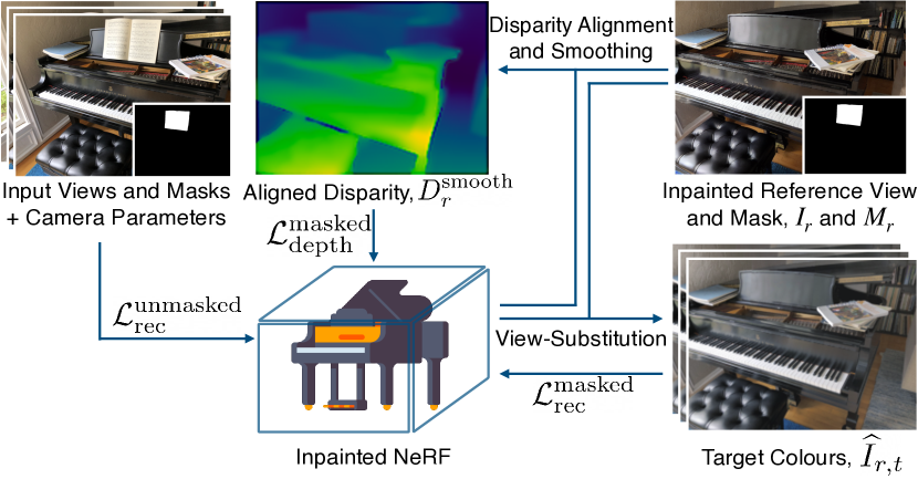
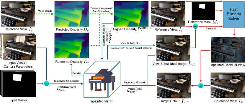
The inputs in our setup are input images, , their camera transform matrices, , and their corresponding masks, 333We assume that masks are given, but they can be obtained automatically with interactive 3D segmentation methods [42, 54]., delineating the unwanted region. We assume a single inpainted reference view, , where , which provides the information that a user expects to be extrapolated into a 3D inpainting of the scene. We propose an approach to use , not only to inpaint the NeRF, but also to generate 3D details and VDEs from other viewpoints as well. In § 4.1, we introduce the use of monocular depth estimators to guide the geometry of the inpainted region, according to the depth of the reference image, . In § 4.2, we propose the use of bilateral solvers [4], in conjunction with our view-substitution technique, to add VDEs to views other than the reference view. See Fig. 2 for a depiction of our geometry supervision and VDE handling. Since not all the masked target pixels are visible in the reference, in § 4.3, we devise an approach to provide supervision for such disoccluded pixels, via additional inpaintings.
Complete Loss Function. Our overall objective for inpainted NeRF fitting is given by:
| (2) |
where , , , and represent the unmasked appearance loss, masked geometry loss, view-dependent masked colour loss, and disocclusion loss, respectively (detailed below). The latter three loss terms have weights , , and . Note that the supervision for , , and are computed every , , and iterations (and hence those losses are not utilized until that many iterations have passed).
4.1 Supervising Reference View Geometry
In the first stage of our algorithm, is supervised on the unmasked pixels for iterations, via the standard NeRF reconstruction loss:
| (3) |
where is the set of rays corresponding to the pixels in , and is the GT colour for the ray, . As a result, while the geometry and appearance of the unmasked parts of the scene begin to converge, the masked region remains under-fit (the masked area is not fit via at this point, as it makes altering masked values in later stages more difficult). The only available guidance for such masked pixels resides in ; however, this only provides single-view appearance information, which cannot directly contribute geometric supervision.
Masked Reference Disparity. To address this challenge, we propose the use of a monocular depth estimator [52, 51], , to predict the uncalibrated disparity of the source view, , and guide the geometry. However, the predicted reference depth, , is non-metric, resides in a different coordinate system, and may be inaccurate, as it was predicted from a single frame. As a result, before supervising the disparity of the NeRF using , we need to align to our rendered NeRF reference disparity, . Although under-fit on the masked pixels, has reliable values for the unmasked pixels.
However, not all of the masked pixels are equally important: areas close to the mask boundary need to be tightly aligned, to ensure the mask edge is minimally visible in the final results, whereas it is not critical to completely align the depths far from the mask, since only the masked pixels will receive supervision with the aligned reference disparity. Thus, we propose to align and for the reference view on the unmasked pixels in a weighted manner, giving higher weight to the points closer to the mask.
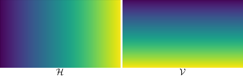
Weighted Disparity Alignment. Traditionally, a scale and an offset are used to affinely transform 2.5D disparity maps, , to [52], where and are the height and width of the input images, and is an all-one matrix. We further increase the degrees of freedom of the alignment to have a tighter alignment around the mask edges. We use two additional matrices, and , where for a pixel , and . Intuitively, these enable additional axis-aligned “tilts” that improve fitting quality. Please see our supplementary material for an illustration of and . Then, the aligned predicted inverse depth is:
| (4) |
Since the pixels closer to the mask are more important for our inpainting application, we use the following weighted objective function to solve for the scalars, :
| (5) |
where is an unmasked pixel from the source view, and is the weight of , which is the inverse of the distance between and the mask centre-of-mass.
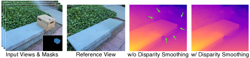
While has significantly improved alignment, misalignments still tend to persist near the edges of . We thus conduct an additional optimization step, where we correct to encourage greater smoothness around the mask, yielding (details in the supplementary material).
Loss. After alignment and smoothing, supervises the masked region of the reference view, , via:
| (6) |
Note that , is recalculated every iterations to utilize the latest fitted geometry, .
4.2 View-dependent Effects by View-substitution
Now that the inpainted region is being geometrically supervised by the depth loss, , we can also supervise the NeRF appearance in the masked region with (see § 4.2.3). Here, we detach the gradients of the densities to prevent the colour loss from affecting the geometry. However, supervision within the masked region from alone does not account for view-dependent changes (e.g., specularities and non-Lambertian effects). To correct this, we propose an approach that enables adding view-dependent effects (VDEs) to the masked area from non-reference viewpoints, by correcting reference colours to match the surrounding context of the other views.
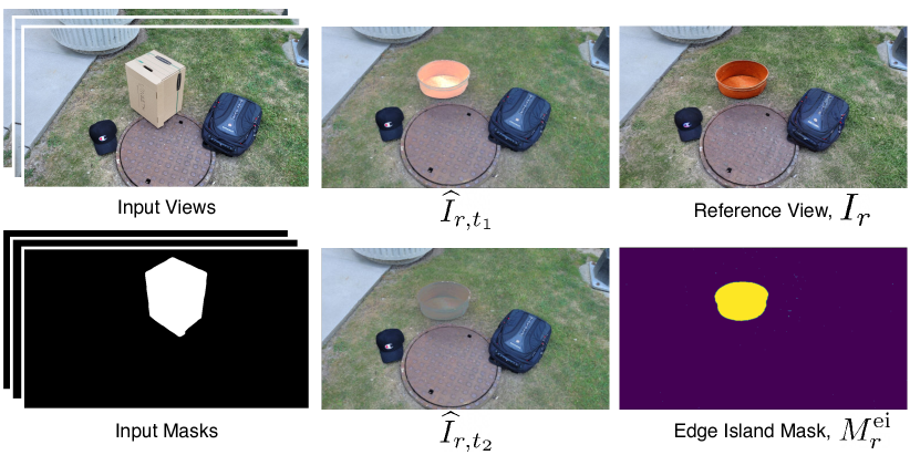
In this section, we consider a target view, . First, in § 4.2.1, we propose our view-substitution method, to enable rendering the scene from the reference camera, but with the colours of . Then, we inpaint the residual between this target-colour render and , propagating the image context of into the masked area, including VDEs (§ 4.2.2). Finally, this residual is applied to obtain corrected reference colours, which are used in § 4.2.3 to supervise the NeRF in masked areas of .
4.2.1 View-substitution
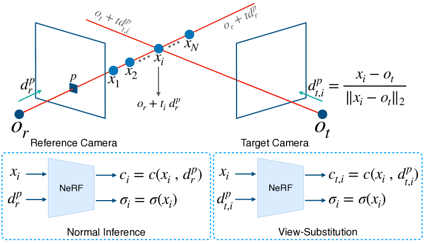
Our view-substitution technique enables looking at the scene from the reference viewpoint, while changing the shading point colours (i.e., in Eq. 1) during rendering to have the colours of a target view. Intuitively, this allows us to construct multiple “versions” of the reference view, each with colours corresponding to the VDEs of a target view.
Fig. 4 shows an overview of our view-substitution method. Consider a pixel, , from the reference view, . During standard NeRF rendering, a ray is cast through the scene, passing from the camera origin, , through the pixel, . This ray is parameterized as , with direction . Next, shading points are sampled on this ray. Normally, for the -th sample on the ray, its coordinates, , and the view-direction, , are fed to the NeRF model to obtain the density, , and the colour from the reference viewpoint, . However, here, instead of the reference view colours, we are interested in the colours of the points as if they were viewed from the target camera. As a result, when computing the shading point colour, we substitute the view direction, , for the direction acquired by connecting the origin of the target view, , and the shading point, . This direction is computed via:
| (7) |
resulting in view-substituted shading point colours instead. We can then volume render from the reference viewpoint across pixels, but with the view-substituted target colours, to obtain rendered images . Such images have the structure of the reference view (e.g., edges), but the appearance (and thus VDEs) of the target view. Please see our supplementary material for additional details and visualizations.
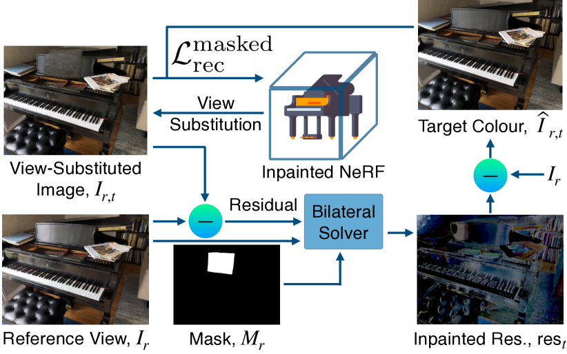
4.2.2 Bilateral Solver for Residuals
At this point, before any supervision on the masked areas of the target images has begun, the view-substituted rendering, , will likely be under-fit inside the mask, , but should have meaningful colours outside of the mask (see Fig. 5, top-left). Consider the residual, , which measures the difference between the reference and target colours (from the reference viewpoint). We want to use the values of this residual outside the mask to predict plausible values for the residual inside of the mask. We rely on the assumption that VDEs (encapsulated by the residuals) cannot have high-frequency variations when there is no edge in the reference view, . In other words, if there is little image contrast in a given region of , we only expect smooth changes in the VDEs of . This is a natural assumption, as changes in materials and reflectance properties are usually accompanied by image edges, demarcating the boundaries between objects or object parts. The bilateral solver [4], denoted , is thus an intuitive approach to inpainting the residual inside the mask, as it enables directly using the edges of for guidance. Briefly, optimizes an image signal, balancing confidence-weighted reconstruction fidelity and bilateral smoothness, guided by the structure of an additional RGB reference image. This is analogous to “diffusing” in pixel values from outside the mask [1], directed by the reference. In our case, thus utilizes as the reference input (from which the edge guidance occurs through the bilateral affinities), while using as the target (valid only outside the mask). We set the confidence to the maximum possible value () outside of the mask and to zero inside it. Then, we run to get the inpainted residual:
| (8) |
The target colours are then obtained as . Note that equals outside the mask, but we only need its values inside the mask for supervision. To ensure this supervision remains up-to-date with the changing NeRF, every iterations, we re-render the view-substituted images, run , and compute (with ).
4.2.3 Supervision from the Reference View
Once the view-substituted (§ 4.2.1) and bilaterally inpainted (§ 4.2.2) target renders, , are available (after reaching at least once), we are now able to supervise the masked appearances of the target images. Note that each such image looks at the scene via the reference source camera (i.e., has the image structure of ), but has the colours (in particular, VDEs) of . We utilize those colours, obtained by the bilateral solver, to supervise the target view appearance under the mask. To do so, we render each view-substituted image inside the mask (obtaining , as in § 4.2.1), and compute a reconstruction loss by comparing it to the bilaterally inpainted output, :
| (9) |
where is the set of rays corresponding to the masked pixels in the reference view (). Fig. 5 provides an overview of our VDE-handling component.
Filtering Edge Islands. Sometimes it is not possible for the bilateral solver, , to propagate values from outside the mask to certain areas on the inside of it. This occurs whenever there is an “edge island” in the masked region: i.e., a disconnected area in bilateral space (e.g., see [38]), such that information from outside the mask will not be transmitted inside. This typically leads to out-of-distribution values in the output from . Here, our goal is to remove such values from consideration. Our approach roughly corresponds to imposing a Lambertian prior on object appearance, to which we default when is too uncertain; in such cases, the target colours will likely end up close to those of the reference view (though this is not guaranteed, due to the view-dependent MLP). To implement this strategy, we detect and filter out-of-distribution values associated to rays in , when calculating Eq. 9, from every target view ; see our supplement for details.
4.3 Disoccluded Regions
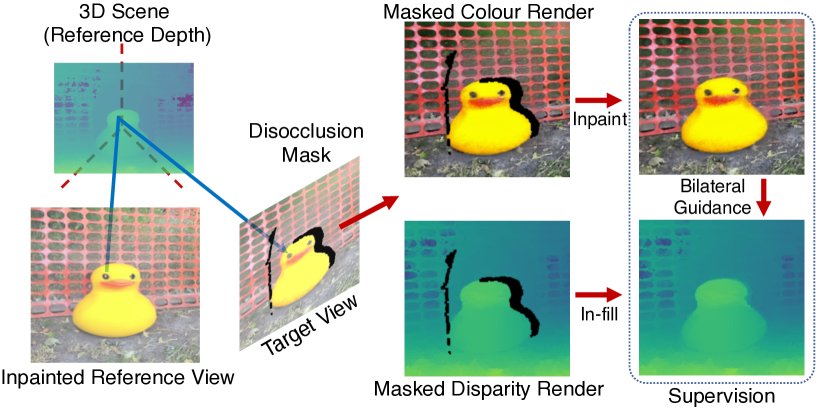
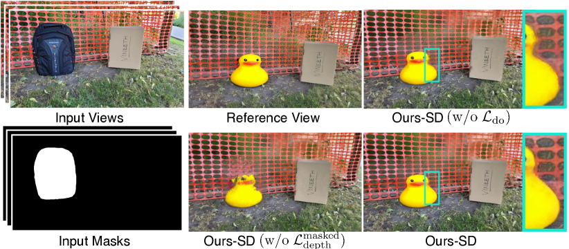
While single-reference inpainting prevents problems incurred by view-inconsistent inpaintings, it is missing multiview information in the inpainted region. For example, when inserting a duck into the scene, viewing the scene from another perspective naturally unveils new details on and around the duck, due to disocclusions (see Fig. 6). We provide an approach to construct these missing details.
Given the inpainted posed reference view, (, ), and a target image, (, ), we first identify the disoccluded pixels in within the mask . Given the reference disparity image, , we unproject every pixel, , into the 3D scene, and then reproject it into , with pixel location . Every masked pixel in that does not receive a projected point (i.e., s.t. ) is disoccluded; i.e., there is no corresponding pixel in to provide appearance information. We therefore obtain a disocclusion mask, , associated to . Next, we inpaint the NeRF render associated to , denoted , masked by : . Finally, we render the disparity image, , and in-fill it as well: , where the bilateral solver, , is guided by the affinities from and confidences from . Similar to § 4.1 and § 4.2, we recompute and every iterations. For fitting, we use the set of rays from through disoccluded pixels in , denoted (i.e., is masked by ). Over a set of cameras, , the following loss is then used:
| (10) |
where , , and colour and disparity are and .
5 Experiments
Datasets. Following SPIn-NeRF [42], we focus on forward-facing scenes, as they are more challenging for the inpainting task. For quantitative evaluations, we use the SPIn-NeRF [42] dataset, which was designed specifically for 3D inpainting. It contains 10 scenes, each with 60 training views (with the object to be removed), 40 test views (without the object), and human-annotated object masks per view. For qualitative examples, we adopt forward-facing LLFF scenes [40, 72] and the SPIn-NeRF dataset [42]. We use simple per-scene text prompts to generate inpainted reference views using Stable Diffusion Inpainting v2 [55]; see our supplementary material for details.
Metrics. Given the ill-posed nature of the task, we follow the 2D [61] and 3D [42] inpainting literature by evaluating the perceptual quality and realism of the inpainted scenes. We conduct experiments based on two types of metrics: full-reference (FR) and no-reference (NR). For FR, we compare the inpainted renderings to ground-truth (GT) captures of the scenes without unwanted objects, based on LPIPS [84] and Frechet Inception Distance (FID) [16]. For both LPIPS and FID, we only compare the inside of the object bounding boxes, matching SPIn-NeRF’s [42] setup. For NR, we assess image quality, without using GT captures, by measuring sharpness via the Laplacian variance [48] and MUSIQ [25], which uses a learned model of visual quality; see our supplementary material for details.
Baselines. We benchmark our approach against six 3D inpainting models. (i) NeRF + LaMa (2D): a NeRF is fit to the scene (including the target object), followed by rendering and inpainting via LaMa [61] from the test views. (ii) Object-NeRF [78] directly removes masked points in 3D, but does not leverage inpainters to clean up disoccluded regions. (iii) Masked NeRF simply ignores the masked pixels during fitting, relying on the NeRF model itself to interpolate the missing values. (iv) NeRF-In [34] uses 2D inpainters as well, including on depth images, but relies on a pixelwise error for fitting, despite multiview inconsistencies. Two versions of (iv), using single and multiple inpainted references, are evaluated. (v) SPIn-NeRF [42] uses a perceptual loss to account for view inconsistencies. We consider two versions with different 2D inpainters, namely Stable Diffusion (SD) [55] and LaMa [61]. (vi) We also consider a variant of Masked NeRF, with an additional loss based on the recent DreamFusion [49, 63] model, which utilizes the SD likelihood as a prior for generating textured 3D models. For i, ii, iii, iv, and v we show the results reported in [42]. See supplementary material for further details.
| Method | LPIPS | FID |
|---|---|---|
| NeRF + LaMa (2D) [61] | 0.5369 | 174.61 |
| Object NeRF [78] | 0.6829 | 271.80 |
| (Masked NeRF) [41] | 0.6030 | 294.69 |
| + DreamFusion [49] | 0.5934 | 264.71 |
| NeRF-In (multiple) [34] | 0.5699 | 238.33 |
| NeRF-In (single) [34] | 0.4884 | 183.23 |
| SPIn-NeRF-SD [42] | 0.5701 | 186.48 |
| SPIn-NeRF-LaMa [42] | 0.4654 | 156.64 |
| \hdashlineOurs-SD | 0.4532 | 116.24 |
| Method | Sharpness | MUSIQ |
|---|---|---|
| SPIn-NeRF-LaMa [42] | 354.31 | 58.10 |
| Ours-LaMa | 394.55 | 62.00 |
| Ours-SD | 398.56 | 61.47 |
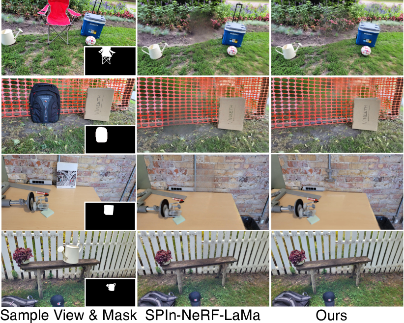
Quantitative Results. In Table 1, we see that our approach provides the best performance on both FR metrics. The Object-NeRF and Masked-NeRF approaches, which perform object removal without altering the newly revealed areas, perform the worst. Combining Masked-NeRF with DreamFusion performs slightly better. This indicates some utility of the diffusion prior; however, while DreamFusion can generate impressive 3D entities in isolation, it does not produce sufficiently realistic outputs for inpainting real scenes. SPIn-NeRF-SD obtains a similar poor LPIPS, though with better FID. It is unable to cope with the greater mismatches of the SD generations. NeRF-In outperforms the aforementioned models. Still, the use of a pixelwise loss leads to blurry outputs. Finally, our model outperforms the second-best model (SPIn-NeRF-LaMa) considerably in terms of FID, reducing it by 25%.
FR measures are limited by their use of a single GT target image. We therefore also examine NR performance, demonstrating improvements over SPIn-NeRF, in terms of both sharpness (by %) and MUSIQ (by %); see Table 2. This confirms our qualitative observation (see Fig. 7) that our results are considerably sharper and more realistic.
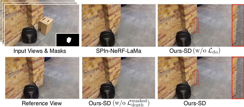
Ablations. In Table 3, we illustrate the effect of ablating components of our algorithm. Using LaMa to obtain led to inferior performance, showing our model benefits from better image inpainters. Further, each of the VDE (§ 4.2), masked depth ( from Eq. 4 in § 4.1), and disocclusion ( from Eq. 10 in § 4.3) handling improve quality. We also include a “gold standard scenario”, where a real photo is used instead of an inpainted one, loosely indicating the best possible score one can expect from the model; this suggests there is room for improvement, simply by improving inpainted reference views. Qualitatively, Fig. 8 illustrates the results of ablating and . The former is harmful to geometric quality (and thus image structure) while the latter blurs outputs in disoccluded areas. Another core contribution is our ability to handle VDEs in non-reference views; ablating our view-substitution-based technique degrades visual quality, as shown in Fig. 9, with uneven and unrealistic brightnesses in novel views. Our supplement contains additional visualizations.
| Method | LPIPS | FID |
|---|---|---|
| Ours-LaMa | 0.4634 | 133.27 |
| Ours-SD (w/o § 4.2 and ) | 0.5279 | 145.60 |
| Ours-SD (w/o ) | 0.5211 | 181.20 |
| Ours-SD (w/o ) | 0.4676 | 126.74 |
| Ours-SD | 0.4532 | 116.24 |
| \hdashlineOurs (w/ GT reference view) | 0.3889 | 104.10 |
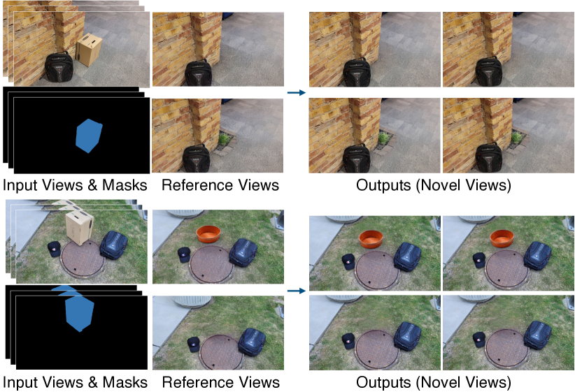
Controllability. An additional major capability of our method is the ability to insert novel content into the 3D scene by providing a different inpainted single-image reference. We refer to this as controllability and showcase examples in Fig. 1. While other methods can also insert content by altering one view, such as using NeRF-In with a single reference, ours (i) avoids visual quality degradation in views far from the reference and (ii) generates non-reference VDEs as well. We demonstrate this in Fig. 10, where we add novel content to each scene, such as the indoor garden and wash basin (see supplemental for more examples). We remark that the expanding generative capacity and creativity of 2D inpainting models, such as text-guided diffusion models (e.g., [55, 50]), will render controllability increasingly important in future work.
6 Conclusion
In this paper, we presented an approach to inpaint NeRFs, via a single inpainted reference image. We used a monocular depth estimator, aligning its output to the coordinate system of the inpainted NeRF to back-project the inpainted material from the reference view into 3D space. We further leveraged bilateral solvers to add VDEs to the inpainted region, and used 2D inpainters to fill disoccluded areas. Our work still has two main limitations: first, we fall back to a diffuse prior in the case of masked edge islands (i.e., when we cannot hallucinate VDEs). Second, exact depth alignment remains difficult. Still, using multiple evaluation metrics, we demonstrated the superiority of our algorithm over prior 3D inpainting methods. We also illustrated the controllability advantage of our model, enabling users to easily alter the generated scene through a single guidance image.
References
- [1] Danny Barash. Fundamental relationship between bilateral filtering, adaptive smoothing, and the nonlinear diffusion equation. TPAMI, 2002.
- [2] Jonathan T. Barron, Ben Mildenhall, Matthew Tancik, Peter Hedman, Ricardo Martin-Brualla, and Pratul P. Srinivasan. Mip-NeRF: A multiscale representation for anti-aliasing neural radiance fields. ICCV, 2021.
- [3] Jonathan T. Barron, Ben Mildenhall, Dor Verbin, Pratul P. Srinivasan, and Peter Hedman. Mip-NeRF 360: Unbounded anti-aliased neural radiance fields. CVPR, 2022.
- [4] Jonathan T Barron and Ben Poole. The fast bilateral solver. In ECCV, 2016.
- [5] Marcelo Bertalmio, Guillermo Sapiro, Vincent Caselles, and Coloma Ballester. Image inpainting. In Conference on Computer Graphics and Interactive Techniques, 2000.
- [6] Anpei Chen, Zexiang Xu, Andreas Geiger, Jingyi Yu, and Hao Su. Tensorf: Tensorial radiance fields. In ECCV, 2022.
- [7] Chaofeng Chen and Jiadi Mo. IQA-PyTorch: Pytorch toolbox for image quality assessment. [Online]. Available: https://github.com/chaofengc/IQA-PyTorch, 2022.
- [8] Zhiqin Chen, Thomas Funkhouser, Peter Hedman, and Andrea Tagliasacchi. MobileNeRF: Exploiting the polygon rasterization pipeline for efficient neural field rendering on mobile architectures. In arXiv, 2022.
- [9] Antonio Criminisi, Patrick Pérez, and Kentaro Toyama. Object removal by exemplar-based inpainting. In CVPR, 2003.
- [10] Angela Dai, Yawar Siddiqui, Justus Thies, Julien Valentin, and Matthias Niessner. SPSG: Self-supervised photometric scene generation from RGB-D scans. In CVPR, 2021.
- [11] Kangle Deng, Andrew Liu, Jun-Yan Zhu, and Deva Ramanan. Depth-supervised NeRF: Fewer views and faster training for free. In CVPR, June 2022.
- [12] Jonas Gehring, Michael Auli, David Grangier, Denis Yarats, and Yann N. Dauphin. Convolutional sequence to sequence learning. In ICML, 2017.
- [13] James Hays and Alexei A Efros. Scene completion using millions of photographs. In SIGGRAPH, 2007.
- [14] Peter Hedman, Pratul P. Srinivasan, Ben Mildenhall, Jonathan T. Barron, and Paul Debevec. Baking neural radiance fields for real-time view synthesis. In ICCV, 2021.
- [15] Philipp Henzler, Niloy J. Mitra, and Tobias Ritschel. Escaping Plato’s cave: 3D shape from adversarial rendering. In ICCV, 2019.
- [16] Martin Heusel, Hubert Ramsauer, Thomas Unterthiner, Bernhard Nessler, and Sepp Hochreiter. GANs trained by a two time-scale update rule converge to a local Nash equilibrium. NeurIPS, 2017.
- [17] Alejandro Ungria Hirte, Moritz Platscher, Thomas Joyce, Jeremy J Heit, Eric Tranvinh, and Christian Federau. Realistic generation of diffusion-weighted magnetic resonance brain images with deep generative models. Magnetic Resonance Imaging, 2021.
- [18] Satoshi Iizuka, Edgar Simo-Serra, and Hiroshi Ishikawa. Globally and locally consistent image completion. ToG, 2017.
- [19] Ajay Jain, Ben Mildenhall, Jonathan T. Barron, Pieter Abbeel, and Ben Poole. Zero-shot text-guided object generation with dream fields. CVPR, 2022.
- [20] Jitesh Jain, Yuqian Zhou, Ning Yu, and Humphrey Shi. Keys to better image inpainting: Structure and texture go hand in hand. In WACV, 2023.
- [21] Jireh Jam, Connah Kendrick, Kevin Walker, Vincent Drouard, Jison Gee-Sern Hsu, and Moi Hoon Yap. A comprehensive review of past and present image inpainting methods. CVIU, 2021.
- [22] Varun Jampani, Huiwen Chang, Kyle Sargent, Abhishek Kar, Richard Tucker, Michael Krainin, Dominik Kaeser, William T Freeman, David Salesin, Brian Curless, and Ce Liu. SLIDE: Single image 3D photography with soft layering and depth-aware inpainting. In ICCV, 2021.
- [23] Ru-Fen Jheng, Tsung-Han Wu, Jia-Fong Yeh, and Winston H Hsu. Free-form 3D scene inpainting with dual-stream GAN. BMVC, 2022.
- [24] Kacper Kania, Kwang Moo Yi, Marek Kowalski, Tomasz Trzciński, and Andrea Tagliasacchi. CoNeRF: Controllable neural radiance fields. In CVPR, 2022.
- [25] Junjie Ke, Qifei Wang, Yilin Wang, Peyman Milanfar, and Feng Yang. Musiq: Multi-scale image quality transformer. In ICCV, 2021.
- [26] Zhengfei Kuang, Fujun Luan, Sai Bi, Zhixin Shu, Gordon Wetzstein, and Kalyan Sunkavalli. PaletteNeRF: Palette-based appearance editing of neural radiance fields. In arXiv, 2022.
- [27] Andreas Kurz, Thomas Neff, Zhaoyang Lv, Michael Zollhöfer, and Markus Steinberger. AdaNeRF: Adaptive sampling for real-time rendering of neural radiance fields. In ECCV, 2022.
- [28] Verica Lazova, Vladimir Guzov, Kyle Olszewski, Sergey Tulyakov, and Gerard Pons-Moll. Control-NeRF: Editable feature volumes for scene rendering and manipulation. In WACV, 2023.
- [29] Wenbo Li, Zhe Lin, Kun Zhou, Lu Qi, Yi Wang, and Jiaya Jia. MAT: Mask-aware transformer for large hole image inpainting. In CVPR, 2022.
- [30] Zuoyue Li, Tianxing Fan, Zhenqiang Li, Zhaopeng Cui, Yoichi Sato, Marc Pollefeys, and Martin R Oswald. CompNVS: Novel view synthesis with scene completion. In ECCV, 2022.
- [31] Chen-Hsuan Lin, Wei-Chiu Ma, Antonio Torralba, and Simon Lucey. BARF: Bundle-adjusting neural radiance fields. In ICCV, 2021.
- [32] David B Lindell, Dave Van Veen, Jeong Joon Park, and Gordon Wetzstein. BACON: Band-limited coordinate networks for multiscale scene representation. In CVPR, 2022.
- [33] Hongyu Liu, Bin Jiang, Yi Xiao, and Chao Yang. Coherent semantic attention for image inpainting. In ICCV, 2019.
- [34] Hao-Kang Liu, I-Chao Shen, and Bing-Yu Chen. NeRF-In: Free-form NeRF inpainting with RGB-D priors. In arXiv, 2022.
- [35] Steven Liu, Xiuming Zhang, Zhoutong Zhang, Richard Zhang, Jun-Yan Zhu, and Bryan Russell. Editing conditional radiance fields. In ICCV, 2021.
- [36] Andreas Lugmayr, Martin Danelljan, Andres Romero, Fisher Yu, Radu Timofte, and Luc Van Gool. Repaint: Inpainting using denoising diffusion probabilistic models. In CVPR, 2022.
- [37] Ziwei Luo, Fredrik K Gustafsson, Zheng Zhao, Jens Sjölund, and Thomas B Schön. Image restoration with mean-reverting stochastic differential equations. arXiv, 2023.
- [38] Nicolas Märki, Federico Perazzi, Oliver Wang, and Alexander Sorkine-Hornung. Bilateral space video segmentation. In CVPR, 2016.
- [39] Nelson Max and Min Chen. Local and global illumination in the volume rendering integral. Technical report, Lawrence Livermore National Lab (LLNL), Livermore, CA (United States), 2005.
- [40] Ben Mildenhall, Pratul P. Srinivasan, Rodrigo Ortiz-Cayon, Nima Khademi Kalantari, Ravi Ramamoorthi, Ren Ng, and Abhishek Kar. Local light field fusion: Practical view synthesis with prescriptive sampling guidelines. ToG, 2019.
- [41] Ben Mildenhall, Pratul P. Srinivasan, Matthew Tancik, Jonathan T. Barron, Ravi Ramamoorthi, and Ren Ng. NeRF: Representing scenes as neural radiance fields for view synthesis. In ECCV, 2020.
- [42] Ashkan Mirzaei, Tristan Aumentado-Armstrong, Konstantinos G. Derpanis, Jonathan Kelly, Marcus A. Brubaker, Igor Gilitschenski, and Alex Levinshtein. SPIn-NeRF: Multiview segmentation and perceptual inpainting with neural radiance fields. In CVPR, 2023.
- [43] Ashkan Mirzaei, Yash Kant, Jonathan Kelly, and Igor Gilitschenski. LaTeRF: Label and text driven object radiance fields. In ECCV, 2022.
- [44] Thomas Müller, Alex Evans, Christoph Schied, and Alexander Keller. Instant neural graphics primitives with a multiresolution hash encoding. TOG, 2022.
- [45] Alexander Quinn Nichol, Prafulla Dhariwal, Aditya Ramesh, Pranav Shyam, Pamela Mishkin, Bob McGrew, Ilya Sutskever, and Mark Chen. GLIDE: Towards photorealistic image generation and editing with text-guided diffusion models. In ICML, 2022.
- [46] Adam Paszke, Sam Gross, Francisco Massa, Adam Lerer, James Bradbury, Gregory Chanan, Trevor Killeen, Zeming Lin, Natalia Gimelshein, Luca Antiga, Alban Desmaison, Andreas Kopf, Edward Yang, Zachary DeVito, Martin Raison, Alykhan Tejani, Sasank Chilamkurthy, Benoit Steiner, Lu Fang, Junjie Bai, and Soumith Chintala. PyTorch: An imperative style, high-performance deep learning library. In NeurIPS, 2019.
- [47] Deepak Pathak, Philipp Krähenbühl, Jeff Donahue, Trevor Darrell, and Alexei Efros. Context encoders: Feature learning by inpainting. In CVPR, 2016.
- [48] Said Pertuz, Domenec Puig, and Miguel Angel Garcia. Analysis of focus measure operators for shape-from-focus. Pattern Recognition, 2013.
- [49] Ben Poole, Ajay Jain, Jonathan T. Barron, and Ben Mildenhall. DreamFusion: Text-to-3D using 2D diffusion. In ICLR, 2023.
- [50] Aditya Ramesh, Prafulla Dhariwal, Alex Nichol, Casey Chu, and Mark Chen. Hierarchical text-conditional image generation with CLIP latents. arXiv preprint arXiv:2204.06125, 2022.
- [51] René Ranftl, Alexey Bochkovskiy, and Vladlen Koltun. Vision transformers for dense prediction. ICCV, 2021.
- [52] René Ranftl, Katrin Lasinger, David Hafner, Konrad Schindler, and Vladlen Koltun. Towards robust monocular depth estimation: Mixing datasets for zero-shot cross-dataset transfer. TPAMI, 2020.
- [53] Christian Reiser, Richard Szeliski, Dor Verbin, Pratul P. Srinivasan, Ben Mildenhall, Andreas Geiger, Jonathan T. Barron, and Peter Hedman. MERF: Memory-efficient radiance fields for real-time view synthesis in unbounded scenes. In arXiv, 2023.
- [54] Zhongzheng Ren, Aseem Agarwala, Bryan Russell, Alexander G. Schwing, and Oliver Wang. Neural volumetric object selection. In CVPR, 2022.
- [55] Robin Rombach, Andreas Blattmann, Dominik Lorenz, Patrick Esser, and Björn Ommer. High-resolution image synthesis with latent diffusion models. In CVPR, 2022.
- [56] Chitwan Saharia, William Chan, Huiwen Chang, Chris Lee, Jonathan Ho, Tim Salimans, David Fleet, and Mohammad Norouzi. Palette: Image-to-image diffusion models. In SIGGRAPH, 2022.
- [57] Chitwan Saharia, William Chan, Saurabh Saxena, Lala Li, Jay Whang, Emily Denton, Seyed Kamyar Seyed Ghasemipour, Burcu Karagol Ayan, S. Sara Mahdavi, Rapha Gontijo Lopes, Tim Salimans, Jonathan Ho, David J Fleet, and Mohammad Norouzi. Photorealistic text-to-image diffusion models with deep language understanding. In NeurIPS, 2022.
- [58] Sara Fridovich-Keil and Alex Yu, Matthew Tancik, Qinhong Chen, Benjamin Recht, and Angjoo Kanazawa. Plenoxels: Radiance fields without neural networks. In CVPR, 2022.
- [59] Meng-Li Shih, Shih-Yang Su, Johannes Kopf, and Jia-Bin Huang. 3D photography using context-aware layered depth inpainting. In CVPR, 2020.
- [60] Shuran Song, Fisher Yu, Andy Zeng, Angel X Chang, Manolis Savva, and Thomas Funkhouser. Semantic scene completion from a single depth image. In CVPR, 2017.
- [61] Roman Suvorov, Elizaveta Logacheva, Anton Mashikhin, Anastasia Remizova, Arsenii Ashukha, Aleksei Silvestrov, Naejin Kong, Harshith Goka, Kiwoong Park, and Victor Lempitsky. Resolution-robust large mask inpainting with Fourier convolutions. In WACV, 2022.
- [62] Matthew Tancik, Pratul Srinivasan, Ben Mildenhall, Sara Fridovich-Keil, Nithin Raghavan, Utkarsh Singhal, Ravi Ramamoorthi, Jonathan Barron, and Ren Ng. Fourier features let networks learn high frequency functions in low dimensional domains. NeurIPS, 2020.
- [63] Jiaxiang Tang. Stable-dreamfusion: Text-to-3d with stable-diffusion, 2022. https://github.com/ashawkey/stable-dreamfusion.
- [64] Alexandru Telea. An image inpainting technique based on the fast marching method. Journal of Graphics Tools, 2004.
- [65] Ayush Tewari, Justus Thies, Ben Mildenhall, Pratul Srinivasan, Edgar Tretschk, Yifan Wang, Christoph Lassner, Vincent Sitzmann, Ricardo Martin-Brualla, Stephen Lombardi, Tomas Simon, Christian Theobalt, Matthias Niessner, Jonathan T. Barron, Gordon Wetzstein, Michael Zollhoefer, and Vladislav Golyanik. Advances in neural rendering. In SIGGRAPH, 2021.
- [66] I Tolstikhin, O Bousquet, S Gelly, and B Schölkopf. Wasserstein auto-encoders. In ICLR, 2018.
- [67] Shubham Tulsiani, Tinghui Zhou, Alexei A. Efros, and Jitendra Malik. Multi-view supervision for single-view reconstruction via differentiable ray consistency. In CVPR, 2017.
- [68] Ashish Vaswani, Noam Shazeer, Niki Parmar, Jakob Uszkoreit, Llion Jones, Aidan N Gomez, Łukasz Kaiser, and Illia Polosukhin. Attention is all you need. In NeurIPS, 2017.
- [69] Dor Verbin, Peter Hedman, Ben Mildenhall, Todd Zickler, Jonathan T. Barron, and Pratul P. Srinivasan. Ref-NeRF: Structured view-dependent appearance for neural radiance fields. CVPR, 2022.
- [70] Can Wang, Menglei Chai, Mingming He, Dongdong Chen, and Jing Liao. CLIP-NeRF: Text-and-image driven manipulation of neural radiance fields. CVPR, 2022.
- [71] Cairong Wang, Yiming Zhu, and Chun Yuan. Diverse image inpainting with normalizing flow. In ECCV, 2022.
- [72] Qianqian Wang, Zhicheng Wang, Kyle Genova, Pratul Srinivasan, Howard Zhou, Jonathan T. Barron, Ricardo Martin-Brualla, Noah Snavely, and Thomas Funkhouser. IBRNet: Learning multi-view image-based rendering. In CVPR, 2021.
- [73] Yi Wang, Xin Tao, Xiaojuan Qi, Xiaoyong Shen, and Jiaya Jia. Image inpainting via generative multi-column convolutional neural networks. In NeurIPS, 2018.
- [74] Zirui Wang, Shangzhe Wu, Weidi Xie, Min Chen, and Victor Adrian Prisacariu. NeRF–: Neural radiance fields without known camera parameters. In arXiv, 2021.
- [75] Chaohao Xie, Shaohui Liu, Chao Li, Ming-Ming Cheng, Wangmeng Zuo, Xiao Liu, Shilei Wen, and Errui Ding. Image inpainting with learnable bidirectional attention maps. In ICCV, 2019.
- [76] Shaoan Xie, Zhifei Zhang, Zhe Lin, Tobias Hinz, and Kun Zhang. SmartBrush: Text and shape guided object inpainting with diffusion model. arXiv preprint arXiv:2212.05034, 2022.
- [77] Zhaoyi Yan, Xiaoming Li, Mu Li, Wangmeng Zuo, and Shiguang Shan. Shift-net: Image inpainting via deep feature rearrangement. In ECCV, 2018.
- [78] Bangbang Yang, Yinda Zhang, Yinghao Xu, Yijin Li, Han Zhou, Hujun Bao, Guofeng Zhang, and Zhaopeng Cui. Learning object-compositional neural radiance field for editable scene rendering. In ICCV, 2021.
- [79] Shunyu Yao, Tzu Ming Hsu, Jun-Yan Zhu, Jiajun Wu, Antonio Torralba, Bill Freeman, and Josh Tenenbaum. 3D-aware scene manipulation via inverse graphics. NeurIPS, 2018.
- [80] Alex Yu, Ruilong Li, Matthew Tancik, Hao Li, Ren Ng, and Angjoo Kanazawa. PlenOctrees for real-time rendering of neural radiance fields. In ICCV, 2021.
- [81] Alex Yu, Vickie Ye, Matthew Tancik, and Angjoo Kanazawa. pixelNeRF: Neural radiance fields from one or few images. In CVPR, 2021.
- [82] Jiahui Yu, Zhe Lin, Jimei Yang, Xiaohui Shen, Xin Lu, and Thomas S Huang. Generative image inpainting with contextual attention. CVPR, 2018.
- [83] Yu-Jie Yuan, Yang-Tian Sun, Yu-Kun Lai, Yuewen Ma, Rongfei Jia, and Lin Gao. NeRF-editing: geometry editing of neural radiance fields. In CVPR, 2022.
- [84] Richard Zhang, Phillip Isola, Alexei A Efros, Eli Shechtman, and Oliver Wang. The unreasonable effectiveness of deep features as a perceptual metric. In CVPR, 2018.
- [85] Shengyu Zhao, Jonathan Cui, Yilun Sheng, Yue Dong, Xiao Liang, Eric I Chang, and Yan Xu. Large scale image completion via co-modulated generative adversarial networks. In ICLR, 2021.
- [86] Yunhan Zhao, Connelly Barnes, Yuqian Zhou, Eli Shechtman, Sohrab Amirghodsi, and Charless Fowlkes. Geofill: Reference-based image inpainting of scenes with complex geometry. In WACV, 2023.
- [87] Chuanxia Zheng, Tat-Jen Cham, and Jianfei Cai. Pluralistic image completion. In CVPR, 2019.
- [88] Yuqian Zhou, Connelly Barnes, Eli Shechtman, and Sohrab Amirghodsi. Transfill: Reference-guided image inpainting by merging multiple color and spatial transformations. In CVPR, 2021.
Appendix A Summary
We provide additional details about the comparative baselines, against which we benchmark, in Appendix B. Further exposition about our disparity smoothing technique (see § 4.1) and edge island filtering method (see § 4.2.3) is given in Appendix C and Appendix D, respectively. Additional visualizations are shown in Appendix E, including methodological illustrations (§ E.1) and qualitative examples (§ E.2 and § E.3). Technical implementation details, such as hyper-parameter values, are discussed in Appendix F. Finally, further explanation about our choice of evaluation metrics is given in Appendix G. Please also view our supplementary website for additional visualizations, including videos.
Appendix B Baseline Details
B.1 Masked-NeRF + DreamFusion
For the Masked-NeRF + DreamFusion baseline, we use the same per-scene text prompts we used to generate our reference views, to guide the generation of the masked region using the score distillation sampling (SDS) [49] loss. We found that gradually and uniformly decreasing the maximum noise steps, , during fitting, until it equals the minimum noise steps, , at the last iteration, improves quality. We suggest this is because, at first, higher noise levels are effective in the generation of global scene structure, and later, lower noise-levels enable fixing details. Due to the unavailability of DreamFusion’s code and their underlying diffusion model, Imagen [57], we used stable-dreamfusion [63], with Stable-Diffusion [55] as the underlying diffusion model.
B.2 NeRF-In
As in prior work [42], we used our own implementation of NeRF-In [34], due to the unavailability of official code. Besides the primary distinctions with our method, such as the pixelwise loss, the remaining architecture (e.g., the use of NGP [44]) is identical to our method. Note that this induces minor implementation differences from the concurrent technical report of NeRF-In, such as the choice of pretrained 2D inpainting model.
Since NeRF-In considers the effect of varying numbers of reference images, we considered two variants of NeRF-In: using multiple reference images (i.e., inpainting all images, as in SPIn-NeRF [42] and using a single one. By default, we utilize the latter method, as it obtains better overall performance (in both our experiments and those of NeRF-In itself), but report the performance of both models in Table 1.
B.3 Object-NeRF
Following the Object-NeRF [78] model, we can remove objects by simply ignoring the contribution of masked 3D points in the volume rendering process (equivalent to setting in masked regions). This is possible here due to the assumed availability of a 3D mask. Note that we are only utilizing this particular approach to object removal, not the entire Object-NeRF algorithm (i.e., the construction of the NeRF itself is identical to our method).
Appendix C Disparity Smoothing Details
After performing the initial depth alignment (as discussed in § 4.1), we further reduce the misalignments around the edges of the reference mask, , via smoothing the aligned reference disparity, . More specifically, to improve the visual continuity of the reference-view boundary between the aligned masked disparity, , and the unmasked rendered NeRF disparity, , we smooth to get the edge-smoothed disparity, :
| (11) |
where is the smoothed disparity correction obtained by minimizing the following objective:
| (12) |
where for a pixel, , is the set of four neighbouring pixels, and is the weight of the smoothness loss. The first term in Eq. C fits the unmasked pixels of to the difference of the rendered disparity, , and the aligned disparity, . The second term is the smoothness penalty, to smoothly propagate the values of from outside the mask to inside.
Appendix D Edge Island Filtering Details
When propagating appearance information into the masked area, in order to construct view-dependent effects for supervision in non-reference views, recall that the bilateral solver is sometimes unable to provide sensible colour values in some areas of the masked region, due to the presence of “edge islands” (see § 4.2.3). Such areas are isolated patches in bilateral space, for which the bilateral solver cannot effectively produce colour values (see Fig. 11 for instances of this). In this section, we provide additional details on our filtering algorithm for removing these invalid values, so that they are not used for supervision.
First, we dilate the mask, , with kernel size to get the dilated mask, . Then, for each target view, , we find the maximum absolute value of the residual inside and outside :
| (13) |
where is the element-wise absolute value. We denote the mask for the pixels in with absolute values higher than as , where is the filtering threshold. The mask of the edge island is then obtained as the union of the mask of all of the out-of-distribution values among all of the target views:
| (14) |
Fig. 11 shows an example of the effects of an edge island inside the masked region (the orange pan) on the target colours of two example target views, and . As shown in the figure, the bilateral solver has failed to predict correct view-dependent colours for the pan, resulting in extreme behaviour inside the pan. Our proposed edge island filtering successfully detects and removes the outlier values via the edge island mask, .
Appendix E Additional Visualizations
E.1 Methodological Illustrations
Depth Alignment Tilt Matrices. In Fig. 12, we visualize the matrices utilized for tighter depth alignment (see § 4.1). These matrices allow the optimization to tilt the depths, in addition to scaling and shifting them.
Overview. We provide an expanded methodological illustration in Fig. 5, covering our approach to providing geometric supervision in the masked region (§ 4.1) and handling the construction of view-dependent effects in non-reference views (§ 4.2); see also Figs. 2, 4, and 5.
View-Substituted Images. We also provide some examples of view-substituted images (see § 4.2.1) in Fig. 14. Notice that the view-substituted images have identical camera viewpoint (and thus image structure) as the reference image, but different colours, corresponding to the view-dependent visual differences across the non-reference images.
E.2 Additional Ablation Examples
Masked Depth and Disocclusion. We show an additional experimental ablation example in Fig. 15, removing masked depth supervision and disocclusion handling (as in Fig. 8). Removing the former causes significantly damaged geometry (and thus considerable visual artifacts as well), while ablating the latter increases blurriness in the disoccluded region (i.e., around newly unveiled details near the occlusion boundary).
Disparity Smoothing. In Fig. 16, we consider the effect of ablating our disparity smoothing approach (see § 4.1 and Appendix C), utilized for obtaining depth in the masked area and matching it to the surrounding scene geometry. Particularly close to the mask boundary, we see that the unsmoothed geometry has a much more jarring transition between the masked and unmasked areas.
E.3 Qualitative Results
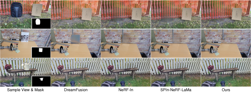
Comparisons. Additional comparisons to SPIn-NeRF, NeRF-In, and DreamFusion are shown for novel view synthesis in Fig. 17. Notice that utilizing the DreamFusion [49] loss along with the Masked-NeRF (see § 5 and Appendix B) can result in unrealistic colours (first row) and sometimes a failure to converge (second row), though the quality improves over Masked-NeRF alone (see Table 1). NeRF-In [34] is blurry in masked areas, as the textures do not match well in a pixelwise manner. SPIn-NeRF [42] reduces this blurriness considerably, but still incurs some level of blur, especially in the presence of more complex textures (e.g., second row). In contrast, our method provides sharp details for all cases.
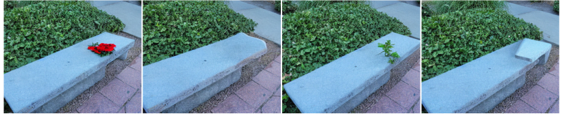
Controllability. We also provide more examples of controllable inpainting in Fig. 18. Notice that we can easily control various aspects of the inpainted scene, such as the presence or absence of roots in the tree (upper rows) or the length of the stone bench (lower rows), by simply changing the inpainting of the single reference image. For additional examples of controllable insertion, see also Fig. 10.
Appendix F Implementation Details
In our experiments, both and are set to . We train each scene for iterations. The disoccusion handling is run every iterations. The weights , , , , and are set to , , , , and , respectively, and is set to . We follow [42] and use a combination of [44] and [11] for faster convergence, and dilate all of the masks for 5 iterations with a kernel to make sure that the masks cover the whole object, and to mask some of the shadows of the unwanted object. All of the images are downsized four times to reduce memory usage and match the experiments of SPIn-NeRF [42]. We also use the distortion loss proposed by [3] for reducing the floater artifacts. We set the weight of the distortion loss to . For generating multiple inpainted source views, we leverage the diversity of denoising diffusion models, and use stable-diffusion inpainting v2 [55]. For inpainting the residuals with the bilateral solver, we set the brightness and colour bandwidths to , while the spatial bandwidth was set to . The strength smoothness and the number of PCG iterations are set to and , respectively. For disocclusion handling, we use LaMa [61] as the 2D inpainter and use three target images for (corresponding to the cameras furthest leftward, rightward, and upward). A small morphological dilation (four iterations with a kernel) is applied to remove noise from the disocclusion masks. The bilateral filter in the disocclusion case uses a spatial bandwidth of only 8. Our implementation is mainly in PyTorch [46]. For generating the inpaintings for Ours-SD, we used stable diffusion inpainting v2 [55], and a simple per-scene text prompt describing the inpainted scene. Below are the text prompts used for SPIn-NeRF scenes:
-
•
A stone bench, a bush in the background, the bench is grey with a rectangular shape in perspective, photorealistic 8k
-
•
A wooden tree trunk on dirt, photorealistic 8k
-
•
A red fence, photorealistic 8k
-
•
Stone stairs, photorealistic 8k
-
•
A circular lid made of rusty iron on a grass ground, photorealistic 8k
-
•
A corner of a brick wall, photorealistic 8k
-
•
A wooden bench in front of a white fence, photorealistic 8k
-
•
An image of nature with grass, bushes in the background, photorealistic 8k
-
•
A desk in front of a brick wall with an iron pipe, photorealistic 8k
-
•
A brick wall, photorealistic 8k
Note that we did not engineer the prompts to improve the results. We typically selected the first generated inpainting. However, as seen in Fig. 2, sometimes, the stable diffusion inpainter adds objects in the scene; in those cases, we regenerated the output to get an inpainting without any additional object for a fair comparison to the baselines. For quantitative experiments, we always select the -th image among the training views in SPIn-NeRF’s dataset [42] as the reference view.
Appendix G Metrics: Additional Details
The ill-posed nature of inpainting means that evaluation is non-trivial: “ground-truth” images are merely one of an infinite number of possible solutions, any plausible member of which should be considered valid. We therefore focus on evaluating perceptual quality and realism, rather than reconstruction, via two types of metrics: full-reference (FR) and no-reference (NR).
In the FR case, we utilize the ground-truth (GT) images of the scene without the object for comparison with LPIPS [84] and Frechet Inception Distance (FID) [16]. LPIPS, a perceptual distance, is far more robust to changes that maintain textural consistency than pixelwise distances. For FID, we compare the distributions of encoded statistics between the inpainted and GT images, which confers high robustness to mismatches in local details, focusing instead on agreement in high-level visual appearance. Both of these metrics were used previously for 3D inpainting evaluation [42]. For both LPIPS and FID, we only perform the comparison inside the bounding boxes of the objects. We expand the bounding boxes by to match SPIn-NeRF’s [42] setup.
However, FR metrics are not completely robust to the choice of reference image, preferring solutions more similar to the GT over others that are equally perceptually realistic. This is exacerbated if an inpainting model inserts new semantic content into a scene, as recent diffusion-based approaches are apt to do (e.g., [55, 50]), whether it is perceptually realistic or not. Thus, we consider two NR metrics, where image quality is assessed in a stand-alone manner. The first measure is simply the variance of the image Laplacian, a classical measure of sharpness (e.g., [48]), which has been previously used to evaluate 2D generative image models [66, 17]. The second is MUSIQ [25, 7], a transformer-based model for NR image quality assessment, meant to reproduce human perceptual judgments.
Note that our metrics in the FR case are computed against bounding boxes (containing the object mask) in held-out views, while our NR sharpness metrics are computed across 120 renders from a camera in a spiralling pattern (in video form). In this way, we assess inpainting quality in its full 3D context; i.e., we ensure that the inpainting quality generalizes to novel views.