Realistic Data Enrichment for Robust Image Segmentation in Histopathology

Abstract

Poor performance of quantitative analysis in histopathological Whole Slide Images (WSI) has been a significant obstacle in clinical practice. Annotating large-scale WSI s manually is a demanding and time-consuming task, unlikely to yield the expected results when used for fully supervised learning systems. Rarely observed disease patterns and large differences in object scales are difficult to model through conventional patient intake. Prior methods either fall back to direct disease classification, which only requires learning a few factors per image, or report on average image segmentation performance, which is highly biased towards majority observations. Geometric image augmentation is commonly used to improve robustness for average case predictions and to enrich limited datasets. So far no method provided sampling of a realistic posterior distribution to improve stability, e.g. for the segmentation of imbalanced objects within images. Therefore, we propose a new approach, based on diffusion models, which can enrich an imbalanced dataset with plausible examples from underrepresented groups by conditioning on segmentation maps. Our method can simply expand limited clinical datasets making them suitable to train machine learning pipelines, and provides an interpretable and human-controllable way of generating histopathology images that are indistinguishable from real ones to human experts. We validate our findings on two datasets, one from the public domain and one from a Kidney Transplant study.

1 Introduction

Large scale datasets with accurate annotations are key to the successful development and deployment of deep learning algorithms for computer vision tasks. Such datasets are rarely available in medical imaging due to privacy concerns and high cost of expert annotations. This is particularly true for histopathology, where gigapixel images have to be processed [34]. This is one of the reasons why histopathology is, to date, a field in which image-based automated quantitative analysis methods are rare. In radiology, for example, most lesions can be characterised manually into clinically actionable information, e.g. measuring the diameter of a tumour. However, this is not possible in histopathology, as quantitative assessment requires thousands of structures to be identified for each case, and most of the derived information is still highly dependent on the expertise of the pathologist. Therefore, supervised Machine Learning (ML) methods quickly became a research focus in the field, leading to the emergence of prominent early methods [25] and, more recently, to high-throughput analysis opportunities for the clinical practice [15, 23, 10]. Feature location, shape, and size are crucial for diagnosis; this high volume of information required makes automatic segmentation essential for computational pathology [15]. The automated extraction of these features should lead to the transition from their time-consuming and error-prone manual assessment to reproducible quantitative metrics-driven analysis, enabling more robust decision-making. Evaluating biopsies with histopathology continues to be the gold standard for identifying organ transplant rejection [22]. However, imbalances and small training sets still prevent deep learning methods from revolutionizing clinical practice in this field.

In this work, we are interested in the generation of training data for the specific case of histopathology image analysis for kidney transplant biopsies. In order to maximize transplant survival rates and patient well-being, it is essential to identify conditions that can result in graft failure, such as rejection, early on. The current diagnostic classification system presents shortcomings for biopsy assessment, due to its qualitative nature, high observer variability, and lack of granularity in crucial areas [32].

Contribution: We propose a novel data enrichment method using diffusion models conditioned on masks. Our model allows the generation of photo-realistic histopathology images with corresponding annotations to facilitate image segmentation in unbalance datasets or cases out of distribution. In contrast to conventional geometric image augmentation, we generate images that are indistinguishable from real samples to human experts and provide means to precisely control the generation process through segmentation maps. Our method can also be used for expert training, as it can cover the extreme ends of pathological representations through manual definition of segmentation masks.

Related Work: Diffusion Models have experienced fast-rising popularity [21, 24, 27]. Many improvements have been proposed [28, 30], some of them suggesting image-to-image transfer methods that can convert simple sketches into photo-realistic images [2]. This is partially related to our approach. However, in contrast to sketch-based synthesis of natural images, we aim at bootstrapping highly performing image segmentation methods from poorly labelled ground truth data.

Data enrichment through synthetic images has been a long-standing idea in the community [33, 19, 9]. So far, this approach was limited by the generative capabilities of auto-encoding [16] or generative adversarial approaches [6]. A domain gap between real and synthetic images often leads to shortcut learning [5] and biased results with minimal gains. The best results have surprisingly been achieved, not with generative models, but with data imputation by mixing existing training samples to new feature combinations [4, 31]. Sample mixing can be combined with generative models like Generative Adversarial Networks (GAN) to enrich the data [19].

2 Method

We want to improve segmentation robustness. We denote the image space as $\mathcal{X}$ and label mask space as $\mathcal{Y}$. Formally, we look for different plausible variations within the joint space $\mathcal{X}\times\mathcal{Y}$ in order to generate extensive datasets $d_{k}=\{(\bm{x}_{n}^{(k)},\bm{y}_{n}^{(k)})\}_{n=1}^{N_{k}}$, where ${N_{k}}$ is the number of labelled data points in the $k$-th dataset. We hypothesise that training a segmentation network $M_{\theta}$ on combinations of $d_{k}$, $d_{a}\cup d_{b}\cup\dots\cup d_{c}$ with or without samples from an original dataset, will lead to state-of-the-art segmentation performance. We consider any image segmentation model $M_{\theta}:\mathcal{X}\rightarrow\mathcal{Y}$ that performs pixel-wise classification, i.e. semantic segmentation, in $\mathbb{R}^{C}$, where $C$ is the number of classes in $\mathcal{Y}$. Thus, predictions for the individual segmentation class labels can be defined as $p(\bm{y}|\bm{x},\theta)=\bm{\hat{y}}=softmax(M_{\theta}(\bm{x}))$.

Inverting the segmentation prediction to $p(\bm{x}|\bm{y},\theta)$ is impractical, as the transformation $M_{\theta}$ is not bijective, and thus inverting it would yield a set of plausible samples from $\mathcal{X}$. However, the inversion can be modelled through a constrained sampling method, yielding single plausible predictions $\bm{\hat{x}}\in\hat{\mathcal{X}}$ given $\bm{y}\in\mathcal{Y}$ and additional random inputs $z\sim\mathcal{N}(0,\sigma)$ holding the random state of our generative process. Modelling this approach can be achieved through diffusion probabilistic models [12].We can thus define $D_{\phi}:\mathcal{Z}\rightarrow\hat{\mathcal{X}}$ where $\mathcal{Z}$ is a set of Gaussian noise samples. This model can be further conditioned on label masks $\bm{y}$ and produce matching elements to the joint space $\mathcal{X}\times\mathcal{Y}$ yielding $D_{\xi}:\mathcal{Z}\times\mathcal{Y}\rightarrow\hat{\mathcal{X}}$.

The first step of our approach, shown in Figure 1, is to generate a set of images $X_{1}=\{\bm{x}^{(1)}_{n}|\bm{x}^{(1)}_{n}=D_{\phi}(z),z\sim\mathcal{N}(0,\sigma)\}\subset\hat{\mathcal{X}}$ where $D_{\phi}$ is an unconditional diffusion model trained on real data samples. We then map all samples $\bm{x}^{(1)}_{n}$ to the corresponding elements in the set of predicted label masks $Y_{1}=\{\bm{y}^{(1)}_{n}|\bm{y}^{(1)}_{n}=M_{\theta}(\bm{x}^{(1)}_{n}),\bm{x}^{(1)}_{n}~{}\in~{}X_{1}\}\subset\hat{\mathcal{Y}}$, where $M_{\theta}$ is a segmentation model trained on real data pairs. This creates a dataset noted $d_{1}$. The second step is to generate a dataset $d_{2}$, by using a conditional diffusion model $D_{\xi}$ trained on real images and applied to the data pairs in $d_{1}$, such that $X_{2}=\{\bm{x}^{(2)}_{n}|\bm{x}^{(2)}_{n}=D_{\xi}(\bm{y}^{(1)}_{n},z),\bm{y}^{(1)}_{n}\in Y_{1},z\sim\mathcal{N}(0,\sigma)\}$. This lets us generate a much larger and more diverse dataset of image-label pairs, where the images are generated from the labels. Our final step is to use this dataset to train a new segmentation model $M_{\zeta}$ that largely outperforms $M_{\theta}$. To do so, we first train $M_{\zeta}$ on the generated dataset $d_{2}$ and fine-tune it on the real dataset.

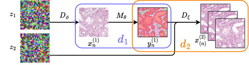
Figure 1: Summary of our dataset generation approach as described in Section 2. We use our diffusion model $D_{\phi}$ to generate images, $M_{\theta}$ segments them and $D_{\xi}$ creates multiple images from these segmentations. Dataset $d_{2}$ is the one used to train our final model $M_{\zeta}$.

Image Generation: Diffusion models are a type of generative model producing image samples from Gaussian noise. The idea is to reverse a forward Markovian diffusion process, which gradually adds Gaussian noise to a real image $\bm{x}_{0}$ as a time sequence $\{\bm{x}_{t}\}_{t=1...T}$. The probability distribution $q$ for the forward sampling process at time $t$ can be written as a function of the original sample image

$$q\left(\mathbf{x}_{t}\mid\mathbf{x}_{0}\right)=\mathcal{N}\left(\mathbf{x}_{t};\sqrt{\bar{\alpha}_{t}}\mathbf{x}_{0},\left(1-\bar{\alpha}_{t}\right)\mathbf{I}\right),q\left(\mathbf{x}_{t}\mid\mathbf{x}_{s}\right)=\mathcal{N}\left(\mathbf{x}_{t};\left(\alpha_{t}/\alpha_{s}\right)\mathbf{x}_{s},\sigma_{t\mid s}^{2}\mathbf{I}\right),$$ (1)

where $\bar{\alpha}_{t}=\sqrt{1/\left(1+e^{-\lambda_{t}}\right)}$ and $\sigma_{t\mid s}^{2}=\sqrt{\left(1-e^{\lambda_{t}-\lambda_{s}}\right)\sigma_{t}^{2}}$ parameterise the variance of the noise schedule, whose logarithmic signal to noise ratio $\lambda_{t}=\log\left(\alpha_{t}^{2}/\sigma_{t}^{2}\right)$ is set to decrease with t [26, 29]. The joint distribution $p_{\theta}$ describing the corresponding reverse process is

$$p_{\theta}\left(\mathbf{x}_{0:T}\right):=p\left(\mathbf{x}_{T}\right)\prod_{t=1}^{T}p_{\theta}\left(\mathbf{x}_{t-1}\mid\mathbf{x}_{t}\right),\quad p_{\theta}\left(\mathbf{x}_{t-1}\mid\mathbf{x}_{t}\right):=\mathcal{N}\left(\mathbf{x}_{t-1};\mathbf{\mu}_{\theta}\left(\mathbf{x}_{t},t,\mathbf{c}\right),\sigma_{t}\right),$$ (2)

where $\mu_{\theta}$ is the parameter to be estimated, $\sigma_{t}$ is given and $\mathbf{c}$ is an additional conditioning variable. Distribution $p$ depends on the entire dataset and is modelled by a neural network. [12] have shown that learning the variational lower bound on the reverse process is equivalent to learning a model for the noise added to the image at each time step. By modelling $\mathbf{x}_{t}=\alpha_{t}\mathbf{x_{0}}+\sigma_{t}\mathbf{\epsilon}$ with $\mathbf{\epsilon}\sim\mathcal{N}(\mathbf{0},\mathbf{I})$ we aim to estimate the noise $\mathbf{\epsilon_{\theta}}(x_{t},\lambda_{t},\mathbf{c})$ in order to minimise the loss function

$$\mathcal{L}=\mathbb{E}_{\mathbf{\epsilon},\lambda_{t},\mathbf{c}}\left[w(\lambda_{t})\left\|\mathbf{\epsilon_{\theta}}(x_{t},\lambda_{t},\mathbf{c})-\mathbf{\epsilon}\right\|^{2}\right],$$ (3)

where $w(\lambda_{t})$ denotes the weight assigned at each time step [13]. We follow [26] using a cosine schedule and DIMM [30] continuous time steps for training and sampling. We further use classifier free guidance [13] avoiding the use of a separate classifier network. The network partly trains using conditional input and partly using only the image such that the resulting noise is a weighted average:

$$\tilde{\mathbf{\epsilon}}_{\theta}\left(x_{t},\lambda_{t},\mathbf{c}\right)=(1+w)\mathbf{\epsilon}_{\theta}\left(x_{t},\lambda_{t},\mathbf{c}\right)-w\mathbf{\epsilon}_{\theta}\left(\mathbf{z}_{\lambda}\right).$$ (4)

The model can further be re-parameterized using v-parameterization [28] by predicting $\mathbf{v}\equiv\alpha_{t}\epsilon-\sigma_{t}\mathbf{x}$ rather than just the noise, $\epsilon$, as before. With v-parameterization, the predicted image for time step $t$ is now $\mathbf{\hat{x}}=\alpha_{t}\mathbf{z}_{t}-\sigma_{t}\mathbf{\hat{v}_{\theta}}(\mathbf{z}_{t})$.

Mask conditioning: Given our proprietary set of histopathology patches, only a small subset of these come with their corresponding segmentation labels. Therefore, when conditioning on segmentation masks, we first train a set of unconditioned cascaded diffusion models using our unlabelled patches. This allows the model to be pre-trained on a much richer dataset, reducing the amount of labelled data needed to get high-quality segmentation-conditioned samples. Conditioning is achieved by concatenating the segmentation mask, which is empty in pre-training, with the noisy image as input into each diffusion model, at every reverse diffusion step. After pre-training, we fine-tune the cascaded diffusion models on the labelled image patches so that the model learns to associate the labels with the structures it has already learnt to generate in pre-training.

Mask Generation: We use a nnU-Net [14] to generate label masks through multi-class segmentation. The model is trained through a combination of Dice loss $\mathcal{L}_{Dice}$ and Cross-Entropy loss $\mathcal{L}_{CE}$. $\mathcal{L}_{Dice}$ is used in combination with a Cross Entropy Loss $\mathcal{L}_{CE}$ to obtain more gradient information during training [14], by giving it more mobility across the logits of the output vector. Additional auxiliary Dice losses are calculated at lower levels in the model. The total loss function for mask generation can therefore be described with

$$\mathcal{L}=\mathcal{L}_{Dice}+\mathcal{L}_{CE}+\beta(\mathcal{L}_{Dice_{1/2}}+\mathcal{L}_{Dice_{1/4}}),$$ (5)

where $\mathcal{L}_{Dice_{1/2}}$ and $\mathcal{L}_{Dice_{1/4}}$ denote the dice auxiliary losses calculated at a half, and a quarter of the final resolution, respectively.

We train two segmentation models $M_{\theta}$ and $M_{\zeta}$. First, for $M_{\theta}$, we train the nnU-Net on the original data and ground truth label masks. $M_{\theta}$ is then used to generate the label maps for all the images in $d_{1}$, the pool of images generated with our unconditional diffusion model $D_{\phi}$. The second nnU-Net, $M_{\zeta}$, is pre-trained on our dataset $d_{2}$ and we fine-tune it on the original data to produce our final segmentation model.

3 Evaluation

Datasets and Preprocessing: We use two datasets for evaluation. The first one is the public KUMAR dataset [18], which we chose to be able to compare with the state-of-the-art directly. KUMAR consists of 30 WSI training images and 14 test images of $1000\times 1000$ pixels with corresponding labels for tissue and cancer type (Breast, Kidney, Liver, Prostate, Bladder, Colon, and Stomach). During training, each raw image is cropped into a patch of $256\times 256$ and then resized to $64\times 64$ pixels. Due to the very limited amount of data available, we apply extensive data augmentation, including rotation, flipping, color shift, random cropping and elastic transformations. However the baseline methods [19] only use 16 of the 30 images available for training.

The second dataset is a proprietary collection of Kidney Transplant Pathology WSI slides with an average resolution of $30000\times 30000$ per slide. These images were tiled into overlapping patches of $1024\times 1024$ pixels. For this work, 1654 patches, classified as kidney cortex, were annotated (glomerulies, tubules, arteries and other vessels) by a consultant transplant pathologist with more than ten years of experience and an assistant with 5 years of experience. Among these, 68 patches, belonging to 6 separate WSI, were selected for testing, while the rest were used for training. The dataset also includes tabular data of patient outcomes and history of creatinine scores before and after the transplant. We resize the $1024\times 1024$ patches down to $64\times 64$ resolution and apply basic shifts, flips and rotations to augment the data before using it to train our first diffusion model. We apply the same transformations but with a higher re-scaling of $256\times 256$ for the first super-resolution diffusion model. The images used to train the second and final super-resolution model are not resized but are still augmented the same. We set most of our training parameters similar to the suggested ones in [26], but use the creatinine scores and patient outcomes as conditioning parameters for our diffusion models.

Implementation: We use a set of three cascaded diffusion models similar to [26], starting with a base model that generates $64\times 64$ images, and then two super-resolution models to upscale to resolutions $256\times 256$ and $1024\times 1024$. Conditioning augmentation is used in super-resolution networks to improve sample quality. In contrast to [26], we use v-parametrization [28] to train our super-resolution models ($64\times 64\rightarrow 256\times 256$ and $256\times 256\rightarrow 1024\times 1024$). These models are much more computationally demanding at each step of the reverse diffusion process, and it is thus crucial to reduce the number of steps during sampling to maintain the sampling time in a reasonable range. We find v-parametrization to allow for as few as 256 steps, instead of 1024 in the noise prediction setting, for the same image quality, while also converging faster. We keep the noise-prediction setting for our base diffusion model, as sampling speed is not an issue at the $64\times 64$ scale, and changing to v-parametrization with 256 time steps generates images with poorer quality in this case. We use PyTorch v1.6 and consolidated [14, 26] into the same framework. Three Nvidia A5000 GPUs are used to train and evaluate our models. All diffusion models were trained with over 120,000 steps. The kidney study segmentation models were trained for 200 epochs and fine-tuned for 25, the KUMAR study used 800 epochs and was fine-tuned for 300. Training takes about 10 days and image generation takes 60 s per image. Where real data was used for fine-tuning this was restricted to 30% of the original dataset for kidney images. Diffusion models were trained with a learning rate of $1\mathrm{e}{-4}$ and segmentation models were pre-trained with a learning rate of $1\mathrm{e}{-3}$ which dropped to $3\mathrm{e}{-6}$ when no change was observed on the validation set in 15 epochs. Through $D_{\phi}$, $M_{\theta}$ and $D_{\xi}$ the number of synthetic samples matched the number of real ones. All models used Adam optimiser. See the supplemental material for further details about the exact training configurations.

Setup: We evaluate the performance of nnU-Net [14] trained on the data enriched by our method. We trained over 5 different combinations of training sets, using the same test set for metrics comparison, and show the results in Table 1. First, we train a base nnU-Net solely on real image data, (1), before fine-tuning it, independently, twice: once with a mixture of real and synthetic images as (2), and once exclusively with synthetic images as (3). The $4^{th}$ and $5^{th}$ models correspond to nnU-Nets retrained from scratch using exclusively synthetic images as (4), and one further fine-tuned on real images as (5) in Table 1.

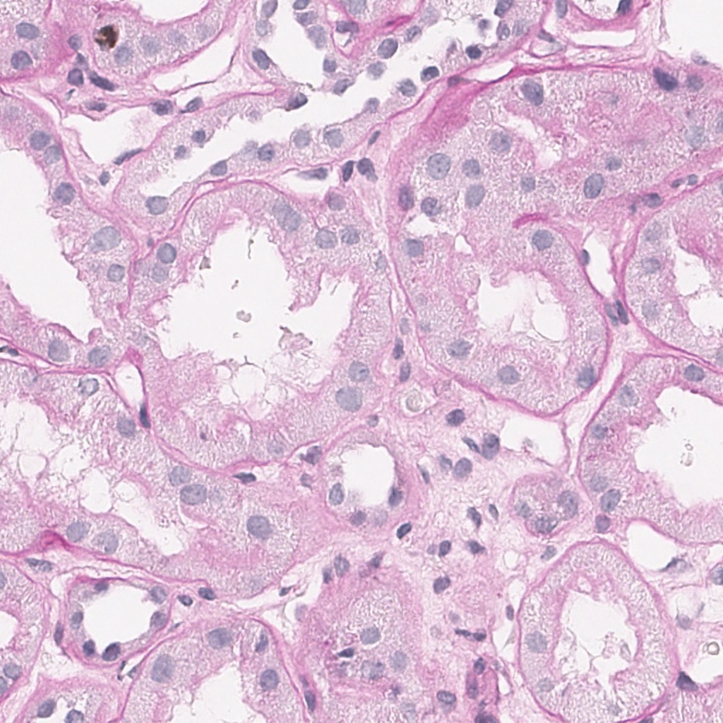
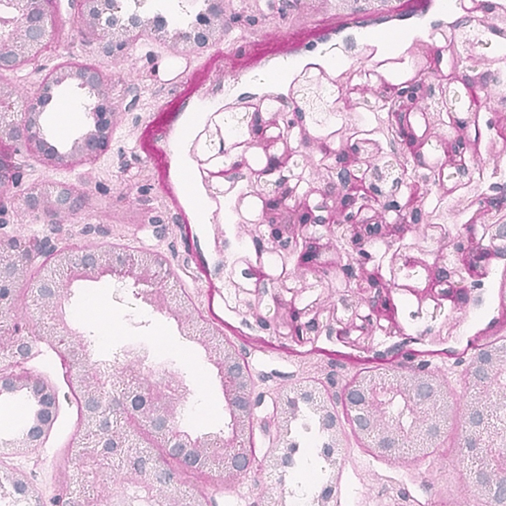
(a) $D_{\phi}$ samp.

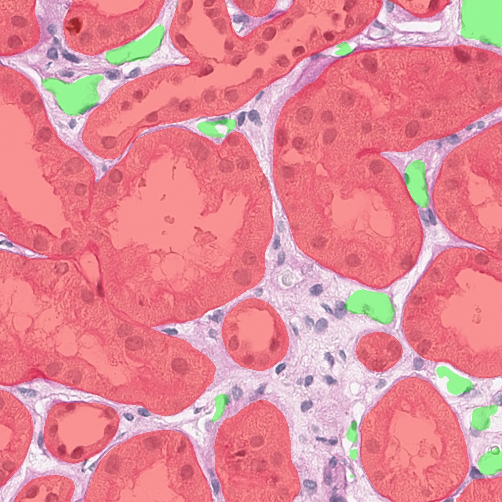
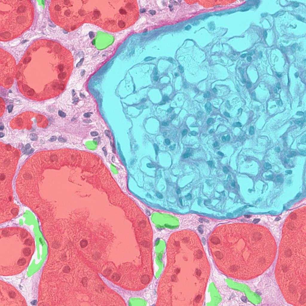
(b) $M_{\theta}$ seg.

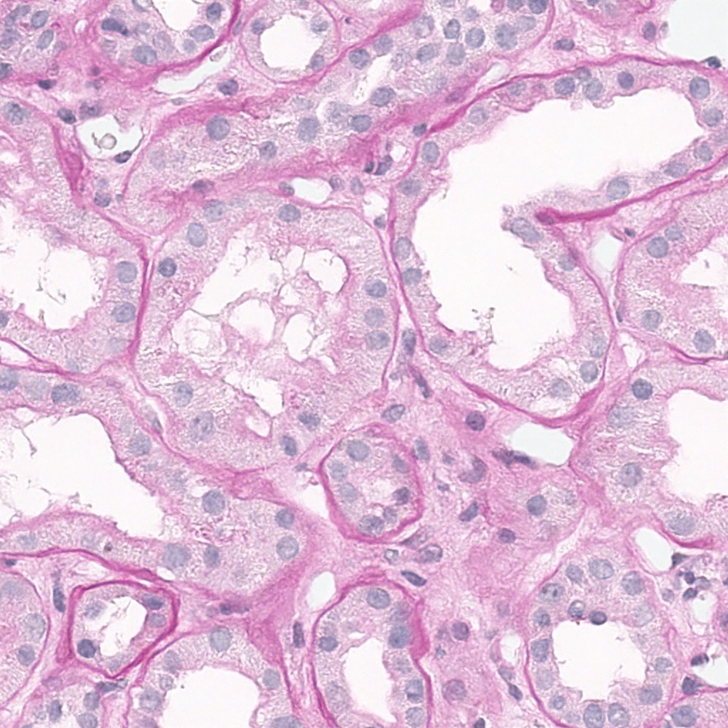
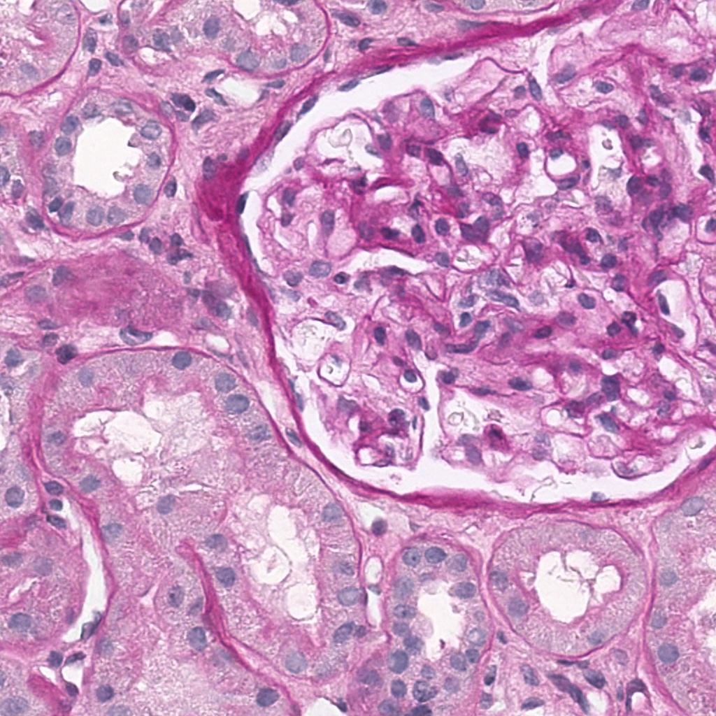
(c) $D_{\xi}$ samp.

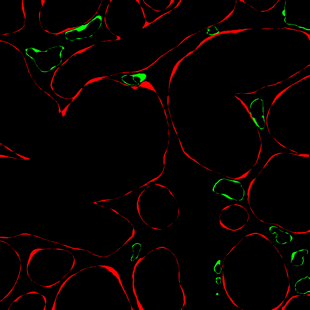
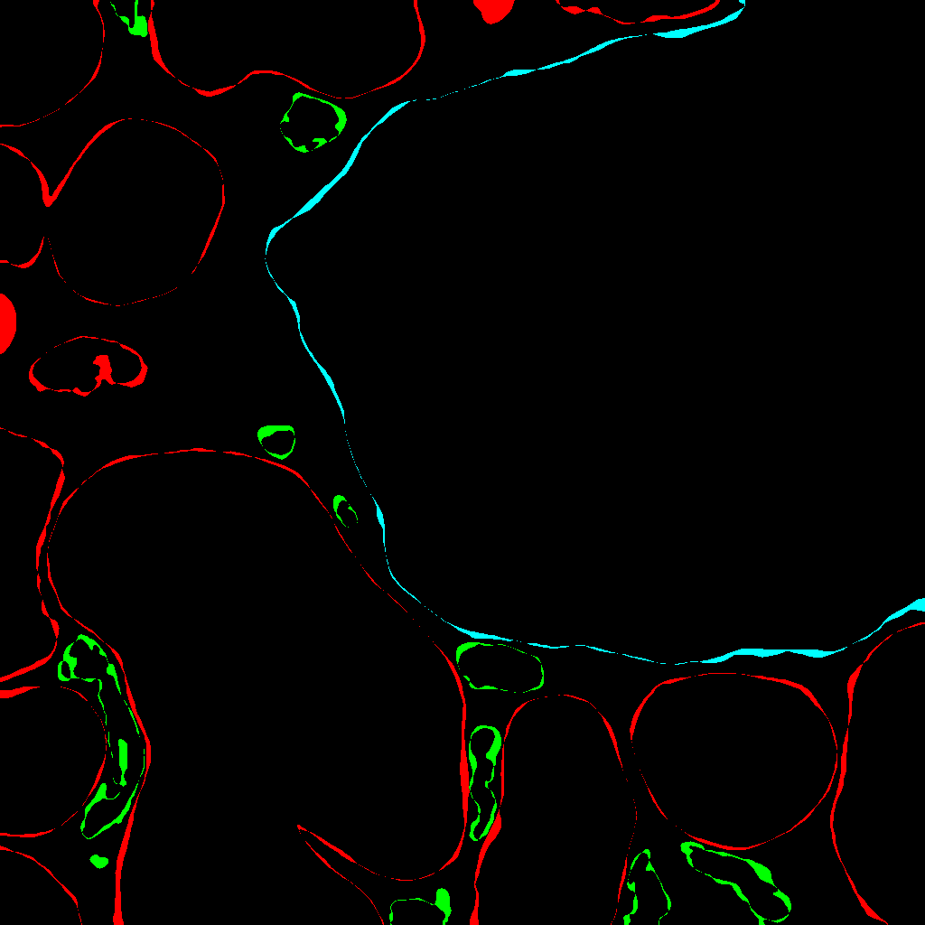
(d) $M_{\zeta}$ -$M_{\theta}$

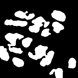
(e)

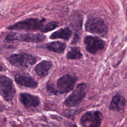
(f)

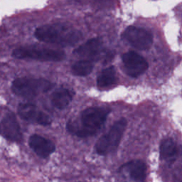
(g)

(h)

Figure 2: Left: Outputs from our models. From left to right: (a) sample from $D_{\phi}$, (b) overlaid segmentation from $M_{\theta}$, (c) sample from $D_{\xi}$, (d) difference map of segmentation from $M_{\zeta}$ and $M_{\theta}$ highlighting shape improvement. Segmentation colors are: red: Tubuli, blue: Glomeruli, green: Vessels. Right: Diffusion model-generated images conditioned on different tissue types in KUMAR, using the same label mask (e). Generated images are from Liver (f), Bladder (g), and Breast (h) tissues. This shows that our conditioning seems to allow a plausible mask to produce any kind of tissue.

Results: Our quantitative results are summarised and compared to the state-of-the-art in Table 1 using the Dice coefficient (Dice) and Aggregated Jaccard Index (AJI) as suggested by [19]. Qualitative examples are provided in Fig. 2 (left), which illustrates that our model can convert a given label mask into a number of different tissue types and Fig. 2, where we compare synthetic enrichment images of various tissue types from our kidney transplant data.

Table 1: Comparison with the state-of-the-art methods on the KUMAR dataset (top) and the limited KIDNEY transplant dataset (bottom). Metrics are chosen as in [19]: Dice and AJI. Best values in bold.

		Method	Dice (%)				AJI (%)
			Seen	Unseen	All		Seen	Unseen	All
KUMAR		CNN3 [17]	82.26	83.22	82.67		51.54	49.89	50.83
		DIST [20]	-	-	-		55.91	56.01	55.95
		NB-Net [3]	79.88	80.24	80.03		59.25	53.68	56.86
		Mask R-CNN [11]	81.07	82.91	81.86		59.78	55.31	57.86
		HoVer-Net [7] (*Res50)	80.60	80.41	80.52		59.35	56.27	58.03
		TAFE [1] (*Dense121)	80.81	83.72	82.06		61.51	61.54	61.52
		HoVer-Net + InsMix [19]	80.33	81.93	81.02		59.40	57.67	58.66
		TAFE + InsMix [19]	81.18	84.40	82.56		61.98	65.07	63.31
	Ours	(1) trained on real	82.97	84.89	83.52		52.34	54.29	52.90
		(2) fine-tuned by synthetic+real	87.82	88.66	88.06		60.79	60.05	60.71
		(3) fine-tuned by synthetic	87.12	87.52	87.24		59.53	58.85	59.33
		(4) trained on synthetic	86.06	89.69	87.10		52.89	58.93	54.62
		(5) trained on synthetic, fine-tuned on real	85.75	87.88	86.36		56.01	57.83	56.5
KIDNEY	Ours	(1) trained on real (30% data)			88.01				62.05
		(2) fine-tuned by synthetic+real			92.25				69.11
		(3) fine-tuned by synthetic			89.65				58.59
		(4) trained on synthetic			82.00				42.40
		(5) trained on synthetic, fine-tuned on real			92.74				71.55

Sensitivity analysis: Out of our 5 models relying on additional synthetic data in the KUMAR dataset experiments, all outperform previous SOTA on the Dice score. Importantly, synthetic results allow for high performance in previously unseen tissue types. Results are more nuanced when it comes to the AJI, as AJI over-penalizes overlapping regions [7]. Additionally, while a further AJI loss was introduced to the final network $M_{\zeta}$, loss reduction, early stopping and the $M_{\theta}$ networks do not take it into account. Furthermore, Table 1 shows that, for the KIDNEY dataset, we can reach high performance (88% Dice) while training $M_{\zeta}$ on $30\%$ (500 samples) of the real KIDNEY data (1). We also observe that the model pretrained on synthetic data and fine-tuned on 500 real images (5), outperforms the one only trained on 500 real images (1). Additionally, we discover that training the model on real data before fine-tuning it on synthetic samples (3) does not work as well as the opposite approach. We argue that pre-training an ML model on generated data gives it a strong prior on large dataset distributions and alleviates the need for many real samples in order to learn the final, exact, decision boundaries, making the learning procedure more data efficient.

Discussion: We have shown that data enrichment with generative diffusion models can help to boost performance in low data regimes, e.g., KUMAR data, but also observe that when using a larger dataset, where maximum performance might have already been reached, the domain gap may become prevalent and no further improvement can be observed, e.g., full KIDNEY data (94% Dice). Estimating the upper bound for the required labelled ground truth data for image segmentation is difficult in general. However, testing model performance saturation with synthetic data enrichment might be an experimental way forward to test for convergence bounds. Finally, the best method for data enrichment seems to depend on the quality of synthetic images.

4 Conclusion

In this paper, we propose and evaluate a new data enrichment and image augmentation scheme based on diffusion models. We generate new, synthetic, high-fidelity images from noise, conditioned on arbitrary segmentation masks. This allows us to synthesise an infinite amount of plausible variations for any given feature arrangement. We have shown that using such enrichment can have a drastic effect on the performance of segmentation models trained from small datasets used for histopathology image analysis, thus providing a mitigation strategy for expensive, expert-driven, manual labelling commitments.

Acknowledgements: This work was supported by the UKRI Centre for Doctoral Training in Artificial Intelligence for Healthcare (EP/S023283/1). Dr. Roufosse is supported by the National Institute for Health Research (NIHR) Biomedical Research Centre based at Imperial College Healthcare NHS Trust and Imperial College London. The views expressed are those of the authors and not necessarily those of the NHS, the NIHR or the Department of Health. Dr Roufosse’s research activity is made possible with generous support from Sidharth and Indira Burman. The authors gratefully acknowledge the scientific support and HPC resources provided by the Erlangen National High Performance Computing Center (NHR@FAU) of the Friedrich-Alexander-Universität Erlangen-Nürnberg (FAU) under the NHR projects b143dc and b180dc. NHR funding is provided by federal and Bavarian state authorities. NHR@FAU hardware is partially funded by the German Research Foundation (DFG) – 440719683. Additional support was also received by the ERC - project MIA-NORMAL 101083647, DFG KA 5801/2-1, INST 90/1351-1 and by the state of Bavarian.

References

- [1] Chen, S., Ding, C., Tao, D.: Boundary-assisted region proposal networks for nucleus segmentation. In: MICCAI 2020, Part V 23. pp. 279–288. Springer (2020)
- [2] Cheng, S.I., Chen, Y.J., Chiu, W.C., Tseng, H.Y., Lee, H.Y.: Adaptively-realistic image generation from stroke and sketch with diffusion model. In: CVPR’23. pp. 4054–4062 (2023)
- [3] Cui, Y., Zhang, G., Liu, Z., Xiong, Z., Hu, J.: A deep learning algorithm for one-step contour aware nuclei segmentation of histopathology images. Medical & biological engineering & computing 57, 2027–2043 (2019)
- [4] Dwibedi, D., Misra, I., Hebert, M.: Cut, paste and learn: Surprisingly easy synthesis for instance detection. In: IEEE ICCV’17. pp. 1301–1310 (2017)
- [5] Geirhos, R., Jacobsen, J.H., Michaelis, C., Zemel, R., Brendel, W., Bethge, M., Wichmann, F.A.: Shortcut learning in deep neural networks. Nature Machine Intelligence 2(11), 665–673 (2020)
- [6] Goodfellow, I., Pouget-Abadie, J., Mirza, M., Xu, B., Warde-Farley, D., Ozair, S., Courville, A., Bengio, Y.: Generative adversarial networks. Communications of the ACM 63(11), 139–144 (2020)
- [7] Graham, S., Vu, Q.D., Raza, S.E.A., Azam, A., Tsang, Y.W., Kwak, J.T., Rajpoot, N.: Hover-net: Simultaneous segmentation and classification of nuclei in multi-tissue histology images. Medical Image Analysis 58, 101563 (2019)
- [8] Graham, S., Vu, Q.D., Raza, S.E.A., Azam, A., Tsang, Y.W., Kwak, J.T., Rajpoot, N.: Hover-net: Simultaneous segmentation and classification of nuclei in multi-tissue histology images. Medical Image Analysis 58, 101563 (2019)
- [9] Gupta, L., Klinkhammer, B.M., Boor, P., Merhof, D., Gadermayr, M.: Gan-based image enrichment in digital pathology boosts segmentation accuracy. In: MICCAI 2019, Part I 22. pp. 631–639. Springer (2019)
- [10] Han, Z., Wei, B., Zheng, Y., Yin, Y., Li, K., Li, S.: Breast cancer multi-classification from histopathological images with structured deep learning model. Scientific reports 7(1), 4172 (2017)
- [11] He, K., Gkioxari, G., Dollár, P., Girshick, R.: Mask r-cnn. In: IEEE ICCV’17. pp. 2961–2969 (2017)
- [12] Ho, J., Jain, A., Abbeel, P.: Denoising diffusion probabilistic models. Advances in Neural Information Processing Systems 33, 6840–6851 (2020)
- [13] Ho, J., Salimans, T.: Classifier-free diffusion guidance. arXiv preprint arXiv:2207.12598 (2022)
- [14] Isensee, F., Jaeger, P.F.: nnU-Net: a self-configuring method for deep learning-based biomedical image segmentation. Nature Methods . https://doi.org/10.1038/s41592-020-01008-z
- [15] Khened, M., Kori, A., Rajkumar, H., Krishnamurthi, G., Srinivasan, B.: A generalized deep learning framework for whole-slide image segmentation and analysis. Scientific reports 11(1), 1–14 (2021)
- [16] Kingma, D.P., Welling, M.: Auto-encoding variational bayes. arXiv preprint arXiv:1312.6114 (2013)
- [17] Kumar, N., Verma, R., Anand, D., Zhou, Y., Onder, O.F., Tsougenis, E., Chen, H., Heng, P.A., Li, J., Hu, Z., et al.: A multi-organ nucleus segmentation challenge. IEEE transactions on medical imaging 39(5), 1380–1391 (2019)
- [18] Kumar, N., Verma, R., Sharma, S., Bhargava, S., Vahadane, A., Sethi, A.: A dataset and a technique for generalized nuclear segmentation for computational pathology. IEEE Transactions on Medical Imaging 36(7), 1550–1560 (2017). https://doi.org/10.1109/TMI.2017.2677499
- [19] Lin, Y., Wang, Z., Cheng, K.T., Chen, H.: Insmix: Towards realistic generative data augmentation for nuclei instance segmentation. In: MICCAI 2022, Part II. pp. 140–149. Springer (2022)
- [20] Naylor, P., Laé, M., Reyal, F., Walter, T.: Segmentation of nuclei in histopathology images by deep regression of the distance map. IEEE transactions on medical imaging 38(2), 448–459 (2018)
- [21] Ramesh, A., Pavlov, M., Goh, G., Gray, S., Voss, C., Radford, Alec, e.a.: Zero-Shot Text-to-Image Generation (February 2021), arXiv:2102.12092
- [22] Reeve, J., Einecke, G., Mengel, M., Sis, B., Kayser, N., Kaplan, B., Halloran, P.: Diagnosing rejection in renal transplants: a comparison of molecular-and histopathology-based approaches. American journal of transplantation 9(8), 1802–1810 (2009)
- [23] Reisenbüchler, D., Wagner, S.J., Boxberg, M., Peng, T.: Local attention graph-based transformer for multi-target genetic alteration prediction. In: MICCAI 2022, Part II. pp. 377–386. Springer (2022)
- [24] Rombach, R., Blattmann, A., Lorenz, D., Esser, P., Ommer, B.: High-Resolution Image Synthesis with Latent Diffusion Models (April 2022), arXiv:2112.10752
- [25] Ronneberger, O., Fischer, P., Brox, T.: U-net: Convolutional networks for biomedical image segmentation. In: MICCAI 2015, Part III 18. pp. 234–241. Springer (2015)
- [26] Saharia, C., Chan, W., Saxena, S., Li, L., Whang, J., Denton, E., Ghasemipour, S.K.S., Ayan, B.K., Mahdavi, S.S., Lopes, R.G., et al.: Photorealistic text-to-image diffusion models with deep language understanding. arXiv preprint arXiv:2205.11487 (2022)
- [27] Saharia, C., Chan, W., Saxena, S., Li, L., Whang, J., Denton, Emily, e.a.: Photorealistic Text-to-Image Diffusion Models with Deep Language Understanding (May 2022), arXiv:2205.11487
- [28] Salimans, T., Ho, J.: Progressive Distillation for Fast Sampling of Diffusion Models (June 2022), arXiv:2202.00512
- [29] Sohl-Dickstein, J., Weiss, E., Maheswaranathan, N., Ganguli, S.: Deep unsupervised learning using nonequilibrium thermodynamics. In: International Conference on Machine Learning. pp. 2256–2265. PMLR (2015)
- [30] Song, J., Meng, C., Ermon, S.: Denoising Diffusion Implicit Models (October 2022), arXiv:2010.02502
- [31] Tan, J., Hou, B., Day, T., Simpson, J., Rueckert, D., Kainz, B.: Detecting outliers with poisson image interpolation. In: MICCAI 2021, Part V 24. pp. 581–591. Springer (2021)
- [32] Van Loon, E., Zhang, W., Coemans, M., De Vos, M., Emonds, M.P., Scheffner, I., Gwinner, W., Kuypers, D., Senev, A., Tinel, C., et al.: Forecasting of patient-specific kidney transplant function with a sequence-to-sequence deep learning model. JAMA Network Open 4(12), e2141617–e2141617 (2021)
- [33] Wang, J., Perez, L., et al.: The effectiveness of data augmentation in image classification using deep learning. Convolutional Neural Networks Vis. Recognit 11(2017), 1–8 (2017)
- [34] Ye, J., Xue, Y., Long, L.R., Antani, S., Xue, Z., Cheng, K.C., Huang, X.: Synthetic sample selection via reinforcement learning. In: MICCAI 2020, Part I 23. pp. 53–63. Springer (2020)