symmetry and Berry phase of bosonic ladder
Abstract
Bose gas on a two-leg ladder exhibits an interesting topological phase. We show the presence of a bosonic symmetry-protected-topological (SPT) phase protected by symmetry. This symmetry leads to fractional quantization of Berry phase, that is a topological order parameter to identify the bulk. Using the Berry phase, we have shown that the interacting bosonic system possesses rich topological phases depending on particle density and strength of interaction. Based on the bulk-edge correspondence, each edge state of the SPT phases is discussed in relation to the Berry phases. Especially we have found an intermediate phase that is not adiabatically connected to a simple adiabatic limit, that possesses unconventional edge states, which we have numerically demonstrate by employing the density-matrix-renormalization group algorithm.
I Introduction
Synthetic dimension in cold atom system constituted by internal states of atom gives a promising platform to simulate and investigate various states of matter Ozawa2019 . An interesting lattice model has already been implemented, such as a two- or three-leg ladder system with an artificial gauge field Mancini2015 ; Stuhl2015 ; Kang2018 ; Han2019 ; Kang2020 ; Han2022 . In coldatom experiments, interacting systems can be implemented and its strength can be controllable Bloch2008 , e.g., Feshbach resonance and using dipole-dipole interactions between dipolar atoms Trefzger2011 ; Baier2016 . In particular, such a system with specific lattice geometry can be used as a quantum simulator to realize rich topological states of matter.
In the community side of the condensed matter theory, symmetry protected topological (SPT) phase is now an attractive state as one of topological states of matter Pollmann2012 . So far, various types of SPT phases have been discovered and also the classification of the SPT phases has been proposed for some groups of the system. The classification for free fermion systems has been explicitly given Altland1997 ; Kitaev2009 ; Ryu2010 (now called “ten-fold way”) and also even for interacting bosonic system. This is listed as a catalog of (bosonic) SPT phases by group cohomology Chen2012 ; Chen2013 . These classification schemes showed possible SPT phases, but demonstration of concrete examples in realistic system is an ongoing problem. In this work, we propose a specific concrete example of an interacting bosonic SPT phase of a two-leg ladder system, feasible in real experiments.
We consider a Bose-Hubbard model with two internal states of atoms, which can be regarded as a two-leg ladder system. Its experimental realization may be easier than that of fermionic one since the system’s temperature of the fermionic system in an optical lattice is somewhat high and it is still a challenging problem to observe a complete quantum long-range order, such as magnetization Mazurenko2017 . We assume that the bosonic model on the two-leg ladder includes on-site and vertical link interactions (interactions between two different internal states), and also a hopping dimerization. Then, a specific type of the bosonic interacting SPT phase appears, characterized by fractional quantization of Berry phase. Due to the two-leg ladder geometry, the system has a key symmetry to induce the SPT phase.
We find that the key symmetry is type, which consists of two types of reflection symmetry combined with time-reversal (complex conjugation). In this work, we show that Berry phase Hatsugai2006 ; Hirano2008 ; Maruyama2009 ; Hatsugai2011 ; Chepiga2013 ; Kariyado2015 ; Maruyama2018 ; Kariyado2018 ; Kawarabayashi2019 ; Mizoguchi2019 ; Araki2020 ; KY_2020 ; Otsuka2021 ; Bunney2022 ; HK2023 can be used as a topological order parameter to characterize the bosonic SPT phase. We analytically show that the Berry phase is fractionally quantized by the presence of the equivalence, as (). The quantization is protected as far as the gap is opened even under a local twist with the symmetry constraints. If the state is adiabatically connected to a set of simple local clusters (plaquette), we may expect the ground state is short-range entangled and topological properties are reduced to those of the simple one. In this work, we numerically demonstrate the presence of the interacting bosonic SPT phases characterized by the fractional quantization of Berry phase coming from equivalence. Due to the Bose Hubbard nature, we find rich SPT phases depending on mean density and strength of interaction. Furthermore, reduction of the equivalence is demonstrated by the quantized Berry phases of . Also an eccentric intermediate phase, that is not the adiabatically connected to the simple clusters, is demonstrated.
In relation to the Berry phase of the bulk SPT phase, we numerically discuss edge states based on the bulk-edge correspondence by using the density matrix renormalization algorithm (DMRG). We shall show some case studies. Depending on the type of edges, mean density and chemical potential, the density profile around the edges significantly varies, that indicate appearance of unconventional edge states. In particular, we numerically find the clear edge density profile, which can be easily identified by higher or lower density than that of the bulk. The appearance of the edge density profile is favorable for the experimental detection of the bosonic SPT phases.
The rest of this paper is organized as follows. In Sec. II, we introduce the target model. In Sec. III, we analytically show the quantization of the Berry phase by equivalence. In Sec. IV, we numerically investigate the presence of the SPT phases in the model, and, in Sec. V, turn into the study of the system with an open boundary case and numerically investigate the presence of the edge state corresponding to the SPT phase in the bulk. We observe the presence of the edge state where the bulk of the system is in SPT phase. Section VI is devoted to discussion and conclusion.
II Model
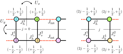
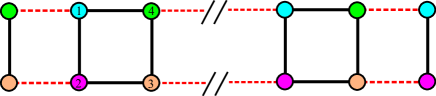
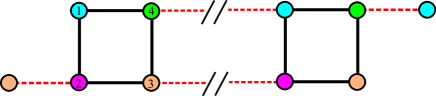
We consider a Bose Hubbard model on two-leg ladder as shown in Fig.1. We start considering the bosonic operator with periodic/open boundary condition with
The Hamiltonian with periodic boundary condition is given by (See Fig.1)
| (1) |
where
where and is the ladder length. is a Hamiltonian at the -th plaquette and connects them. , are hopping amplitudes as shown in Fig. 1, is a chemical potential, and -term is on-site interaction (between same internal states). The -term represents interactions between the upper and lower chain. If the upper and lower chains are created by a different internal state atom in realistic experimental situations such as a synthetic ladder optical lattice Mancini2015 ; Stuhl2015 . The -term can be regarded as interactions between different internal states and the -hopping is Rabi coupling. We also comment that without the synthetic ladder the target system is also feasible in a real experimental system, such a bosonic plaquette optical lattice Paredes2008 ; Nascimbene2012 and also the model with synthetic gauge fields has been theoretically studied Greschner2016 ; Buser2020 . In what follows, we set and and a mean density is used to specify the filling of the system. In most of our work, we focus on a strongly correlated regime, , practically and consider soft-core bosons, where we expect that the ground state is always gapped unique and also any spontaneous symmetry breaking do not occur.
III Symmetry protection and fractional quantization Berry phase
We introduce a equivalence of the Berry phases associated with symmetry (2 reflections) of the ladder due to the hopping pattern and the form of the interaction. This symmetry can be employed to define a specific type of SPT phases. We then introduce a Berry phase by setting local twists on links. This equivalence leads to the fractional quantization of the Berry phase.
In what follows, we shall explain the equivalence and introduce Berry phase. Physical origin of the quantization is special for the ladder compared with the previous studies Hatsugai2006 ; Hirano2008 ; Maruyama2009 ; Hatsugai2011 ; Chepiga2013 ; Kariyado2015 ; Maruyama2018 ; Kariyado2018 ; Kawarabayashi2019 ; Mizoguchi2019 ; Araki2020 ; KY_2020 ; Otsuka2021 ; Bunney2022 .
III.1 symmetry
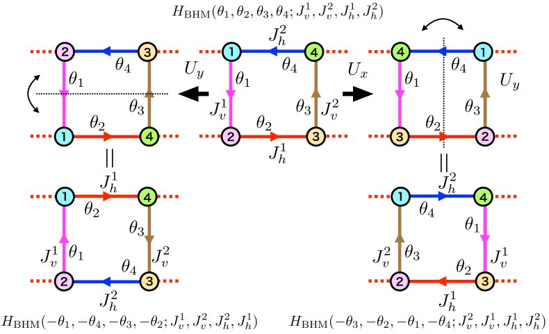
The symmetry constraint to protect a SPT phase we discuss is a combination of two reflections with time-reversal. We consider two unitary operators, and for reflections shown in Fig.1
where two unitary operators and operate for the boson operators as
Note that this symmetry protection is respected for periodic boundary condition and also open boundary condition by cutting the link at the origin ( at the links ). It can guarantee the bulk-edge correspondence associated with Berry phase as discussed later.
III.2 Quantized Berry phase as a topological local order parameter
Let us introduce quantized Berry phase for a generic system by introducing a set of local twists as a parameter set. This type of the quantized Berry phase is a toplogical order parameter of the short-range entangled state Hatsugai2006 ; Hirano2008 ; Hatsugai2011 ; Kariyado2014 ; Kariyado2015 ; Araki2020 . The generic strategy is as follows. By introduction of the local twists as a set of parameters for the Hamiltonian, the Berry phase is defined for a many body ground state. Although, the Berry phase may take any value generically, one may impose symmetry constraints (with the twists), which induces quantization of the Berry phase. Due to the quantization, this quantized Berry phase can not be modified by small but finite perturbation. It implies that the quantized Berry phase is topologically stable and works local topological order parameter of the bulk. Since we need energy gap between the ground state (or set of ground states as a multiplet) and the other, this topological order parameter is only well defined for the gapped ground state. It picks up responses of the many body ground state against for the local twists as “perturbation”. If the system is adiabatically modified (without gap closing) and decoupled into a set of local clusters, the system is short-range entangled. Since introduction of local gauge transformation of the bosonic/fermionic/spin operators inside some specific cluster does not affect the other clusters and induces twists only inside, it characterizes the locality. Using the twists, a Berry phase of the cluster can be defined assuming the ground state of the cluster is unique. Apparently it is also considered as a Berry phase of the total system (although the cluster is decoupled). Also its value is easily evaluated since the twists are gauged out (See example below). Using the same twists, even with finite inter-cluster coupling, one may define a Berry phase associated with the many-body ground state. Note that the twists with the finite inter-cluster coupling can not be gauge out. In generically this Berry phase may take any value in modulo . However, due to symmetries the system possesses with the twists, the Berry phase may need to satisfy several constraints, which may result in the quantization. This is the quantized Berry phase and, then, it works as a topological order parameter of the system. Especially when the inter-cluster coupling is finite but weak enough, this quantized Berry phase is a topological order parameter of the short-range entangle state.
III.3 fractionalization in ladder
Following this strategy, let us define Berry phase for the periodic boundary condition by introducing a set of twists, , only in the plaquette at the origin () as shown in Fig.1 and Fig.2. The modified dependent Hamiltonian, , is given by replacing ,
| (2) |
where , , and .
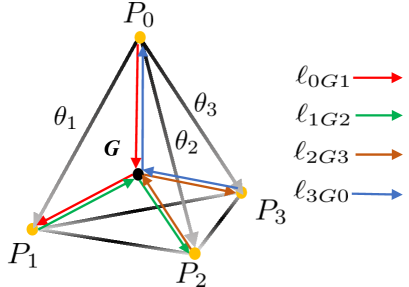
By imposing a constraint , mod , this set of the twists is specified by the point in the 3-torus, as shown in Fig.3. We use this extended notation using 4 parameters to specify 3-torus, which is useful to discuss the symmetry of the ladder (see below).
Identifying the equivalent points, any path connecting the vertices, ’s (), define loops as shown in Fig. 3. Then assuming the ground state is unique (gap remains open) on the loop, the Berry phase is defined as
where is a ground state of ( and is any parameter to specify the loop, . The Berry phase is defined of 4 special paths as
| (3) |
where
| (4) |
As for the twisted Hamiltonian, the reflections , that make the untwisted Hamiltonian invariant, operate as (See Fig.2)
where relevant parameter dependence is explicitly shown. If , the twisted Hamiltonian on the loop is mapped as,
| (5) |
where
It implies
Note that, in general, as for the parameter independent anti-unitary operator , where , the Berry connection of the state is since is pure imaginary. Then using abbreviation, , , , , it is further written as
By using the apparent relation, mod , due to the cancellation of the paths, it is summarized as
| (6) | ||||
| (7) |
It naturally implies a partial quantization,
| (8) |
for any except .
Similarly if , we have following relations,
| (9) |
It implies
and then
It is summarized as
| (10) | ||||
| (11) |
It naturally implies a partial quantization,
| (12) |
for any except .
If the ladder satisfies the full symmetries, and , supplemented with the constraint ,
| (13) |
This is the quantization of the ladder. We call it Berry phase Hatsugai2011 ; HK2023 .
III.4 Plaquette limit
The quantized values, Eq.(8) , Eq.(12) and Eq.(13) are fixed explicitly if the system is adiabatically connected to a set of decoupled plaquette ().
As for the Berry phase, it is enough to consider a single plaquette in this case. The twists are gauge out, (or they are induced) by the gauge transformation (See Eq.(2))
where note that , (). , , , . It implies that .
Noting that , the Berry connection and the Berry phase are given as
where and .
As for the canonical loops, it is
We assume that the ground state of the total system (and thus, that of the plaquette as well) is unique. Then total number of boson in the plaquette is positive integer .
When , due to the invariance by , and . It implies
Also due to this , , that implies the partial quantization,
Similarly, when , due to the invariance by , and . It implies
Also , that implies the partial quantization,
Then when the system is invariant, and , we have quantization as
These quantized Berry phases are adiabatic invariants.
III.5 Another Berry phase
We also consider a set of twists in by assuming the symmetry due to , that is, as
| (14) |
We also consider a Berry phase associated with this set of twists. Due to the symmetry, it is quantized into as
This is due to the symmetry constraint
A dimer limit (, ) is the decoupled limit for this case.
| (15) | |||||
| (16) |
In this decoupled case,
Further and due to the invariance by . It implies . Then adiabatic continuation to this dimer limit guarantees
IV Numerical evaluation of the SPT phase
In the previous section, we showed the fractional quantization of the Berry phase by the symmetry. We herein turn to the numerical demonstration of its fractional quantization in the Hamiltonian by using diagonalization Quspin for various parameter conditions. The fractional quantization of the the Berry phase is the signal of the presence of the bulk SPT phase protected by the symmetry.
In what follows, we set and . We introduce a dimerization parameter as , and set . This setting preserves the symmetry. We focus on and consider soft-core bosons.
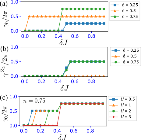
As varying for , and , the Berry phase behaves as shown in Fig. 4 (a). For and and , we observe the fractional quantization and , and the Berry phase captures clear topological phase transitions at . On the other hand, for , the finite fractional quantization appears even for a finite . The reason is that two dimer states resided on -links on a plaquette is adiabatically connected to a plaquette cluster state. These results of the fractional quantization are the signal of the presence of the bulk SPT phases of the symmetry. Also note that the quantization value of the Berry phase is related to the mean density , which is expected by considering a decoupled plaquette limit.
We then calculate the Berry phase. Since the model of has inversion symmetry, thus, the Berry phase can capture a topological phase transition from to Kariyado2015 . Figure 4 (b) is the behavior of the Berry phase. We observe that for and cases, the Berry phase characterizes a topological phase transition and its topological phase but for , the Berry phase does not capture the presence of the bulk SPT phase.
We observe effects of the interaction . The Berry phase exhibits an interesting behavior for as shown in Fig. 4 (c). As varying , we observe an intermediate plateau phase with for a moderate and , this behavior is a specific character in bosonic system Deng2014 ; KSI2017 . This intermediate phase we find is interesting in that, this state is not adiabatically connected to the state of the plaquette limit, which exhibits state.
Next, to observe the importance of the symmetry for the presence of SPT phase, we here introduce a symmetry breaking potential. As a perturbation, we add a potential,
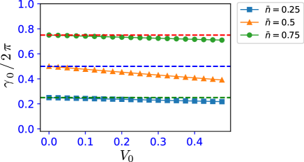
which breaks the symmetry. We expect that as increasing , the fractional quantization of the Berry phase is collapsed. In fact, we verify this expectation as shown in Fig. 5. For each densities , the quantization continuously breaks down as increasing . This result indicates the symmetry is crucial for existing the SPT phase in the bosonic system.
An interesting behavior of the Berry phase in the system with only symmetry is observed ( is broken). From Eqs. (6) and (7), a certain relation of Berry phase exists,
| (17) |
Combined with the relation , one obtain
| (18) |
The sum of the two Berry phases is quantized. We verify this unconventional quantization. To this end, we modify the parameters and as
| (21) |
| (22) |
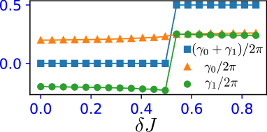
The Hamiltonian is no longer invariant for the symmetry and invariant only for the symmetry . For , we demonstrate the quantization of the sum of the Berry phases. Figure 6 is the numerical result. Depending on the value of , the sum takes or and we observe a clear phase transition while each and take some fractional values for any or do not take . Hence, we confirm the quantization of the sum of the Berry phase as shown in Eq. (18).
In addition, we expect that the bulk SPT phases appear in spinless free fermion system. See Appendix, we confirmed the presence of the SPT phase, which are also characterized by the fractional quantization of the Berry phase.
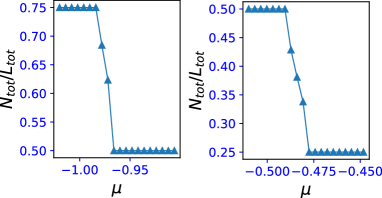
Before going to the next section, we show the DMRG calculation allowing the change of the particle number in the system to consolidate the presence of the bulk SPT phases as shown in Fig.5 (a). We employ the DMRG algorithm by using TeNPy library TeNPy . In the calculation, we vary the chemical potential in the system with the periodic boundary condition. The results are shown in Fig. 7, where the same parameter condition is set as in Fig.4 (a). We find some plateaus with the total particle number constant. The results indicate that the density on each plateau corresponds to that of each bulk SPT phases as shown in Fig.7 (a) and 7 (b), each state on each plateau is gapped and incompressible. This is reminiscent of the appearance of the magnetization plateaus Oshikawa1997 ; Kariyado2015 and the density plateaus of Mott insulator in the conventional Bose Hubbard model Fisher1989 .
V Edge states in bosonic SPT phases
In general, the bulk-edge correspondence is to read out the information of the bulk from various edge states under various forms of edge. Conversely, if a non-trivial bulk state exists, then one introduces an edge in the system and some edge state appears. It is possible to predict the form of edge state from inferring what states appear by cutting the decoupled plaquette in this system.
For the bosonic system in this work, if we believe the presence of the bulk-edge correspondence, some bosonic edge state can appear under some edge shape. However, it is difficult to directly deduce the presence and detailed properties of edge state since our considering bosonic system is complex due to the ladder geometry, the presence of the interactions, the vertical hoppings and soft-core boson nature. It is difficult to identify some symmetries that would characterize the appearance of edge states as they appear in free fermions (cf. chiral symmetry). Even in this situation, when we set an experimentally feasible edge shape of interest, we can confirm numerically on a case-by-case what edge states appear, at least. Thus, we perform such a study in the following.
To detect some edge state, we also employ DMRG algorithm TeNPy . We here impose an open boundary condition and analyze the two cases: (i) a vertical edge case and (ii) a diagonal edge case. For both of cases, we employ the simulation allowing the change of particle number in the system (grand-canonical), that is, vary the chemical potential and observe density properties of both bulk and edges. We expect that edge states (if appear) are different from that of a conventional free-fermion system with a certain topological phase. In particular, we comment that it is care that in general, bosonic systems with open boundary do not necessarily have zero-energy edge state, e.g. due to the lack of chiral symmetry. Some interacting bosonic systems have already reported it and numerically verified in the context of the topological Mott insulator Grusdt2013 and Haldane insulator Stumper2020 .
V.1 Vertical edge case
We first focus on the system with vertical edge as shown in Fig. 8. The edge is simply introduced by cutting a single plaquette at of the periodic system. The boundary preserves both and symmetries.
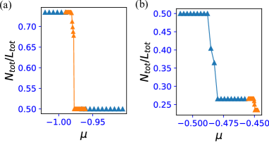
We start to observe the behavior of total density obtained by summing over local density of all sites as varying . The result is shown in Figs. 9 (a) and 9 (b). We observe how the behavior of the total density of the periodic case as shown in Fig. 7 changes by introducing edges. As same to the periodic boundary calculations in Fig. 7, we find some plateaus with the total density constant. For each plateaus, the bulk states correspond to the bulk SPT phases with different Berry phase (the density distribution will be shown in later).
Interestingly, we find two more small plateau regime around , where particle distribution on edges are specific as shown in later.
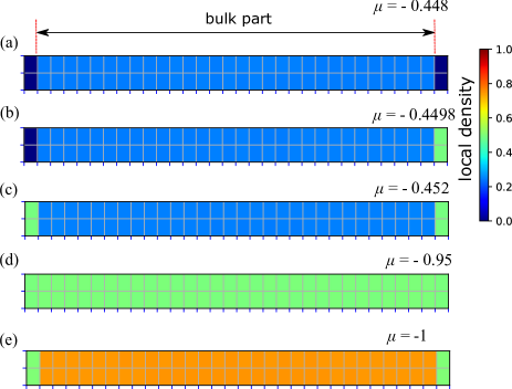
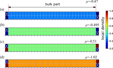
Let us observe the local density distribution for specific ’s on each plateaus and what type of edge state appears. The distribution at in the rightmost small plateau in Fig. 9 (b) is shown in Fig. 10 (a). The bulk part has , corresponding to the phase with and the left and right edge sites shows empty (localized holes). Any bosonic edge state does not appear. Next, we focus on case, this point is in the second rightmost (very) small plateau in Fig. 9 (b). As shown in Fig. 10 (b), we here find that a localized edge state at right edge sites appears. This state is close to a single bonding state forming on the rung of a ladder sim_bonding , . The bulk SPT phase with remains. That is, the whole of the wave function can be written by , where is the bulk SPT state. This edge state is expected from the decoupled plaquette limit for . If we cut the single plaquette into two halves, some bonding-like states can appear. Also we expect that at , the ground state is two-fold degenerate. That is, the state is also another ground state. Here practically our DMRG calculation just choices the right edge state . In fact, note that due to the presence of degenerate states, the true observed local density is obtained by where . Then, the densities of left and right edge sites are all same, .
We next show the distribution at in the third rightmost plateau in Fig. 9 (b) is shown in Fig. 10 (c). There, at both edges the localized edge states appear. Varying induces the additional appearance of the edge state. The bulk SPT remains. The state is .
We further show smaller case. The distribution at in the leftmost plateau in Fig. 9 (b) is shown in Fig. 10 (d). The bulk state changes to , corresponding to the SPT phase with and but remains the edge states at both edges. The state is , where is the SPT with . This numerical result indicates that for the change of around the plateau jumps, , the bulk state changes rather than edge state changes. We expect that the reason is large density fluctuation due to the boson nature. It is difficult to find some types of edge states expected from the decoupled plaquett limit for , compared to the low-density region.
Finally, we observe the distribution at in the left plateau in Fig. 9 (a) is shown in Fig. 10 (e). The bulk part has , corresponding to the phase with . Same to the previous case as shown in Fig. 10 (d), the single edge state remains at both edges. The state is , where is the SPT with . From this result, the bulk state tends to change rather than edge state around the plateau jumps ().
Summarizing the results of the vertical edge case, we observe that the appearance of the edge state close to the bonding state, identified by difference of density from that of the bulk (mean density ), depends on the SPT phase in the bulk with different mean density . In particular, for the bulk SPT with , some types of edge state appears by fine-tuning . These states are predicted from the state of the decoupled plaquette limit.
V.2 Diagonal edge case
We move to the study of the diagonal edge case. The shape of edges is shown in Fig. 11. Note that this edge geometry cannot be obtained by a periodic ladder ring as in the vertical edge as shown in Fig. 8, but is obtained by cutting an infinite ladder. Here the length of the bulk part is , the total number of the lattice site is . In contrast to the vertical edge case, the boundary condition breaks individual and symmetries, but symmetry remains. We focus on the density distribution for each single sites for the case and numerically investigate whether some edge states appear. Under the diagonal edge, the sites on the edges do not couple to another site in the vertical direction, that is, no vertical hopping and interactions, implying that a localized particle edge state or hole around the edges can appear.
We start to observe the behavior of total density obtained by summing over local density of all sites as varying . The result is shown in Fig. 12 (a) and 12 (b). As same to the calculations of periodic boundary condition in Fig. 7, we find some plateaus with the total density constant. For each plateaus the bulk states correspond to the bulk SPT phases with different Berry phase. Interestingly, we find one more plateau around , where particle distribution on edges are specific as shown in later.
We further show some local density distributions for specific ’s on each plateaus. The distribution at in the rightmost plateau in Fig. 12 (b) is shown in Fig. 13 (a). The bulk part has , corresponding to the phase with and single hole appears at the left and right edge sites. A localized particle edge state does not appear. The reason for it is that if such a particle exists for finite , the particle tends to intrude to the bulk part due to the low density, but once the particle enters into the bulk (This is likely to occur due to the low density of the bulk), the state is energetically unstable due to the presence of interactions.
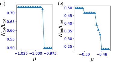
Next we show the distribution at in the middle plateau in Fig. 12 (b) is shown in Fig. 13 (b). The bulk part has , corresponding to the phase with and we observe single hole at the left and right edge sites. However, we further a little decrease , this plateau is swept and another plateau appears. See the distribution at shown in Fig. 13 (c). Although the bulk SPT state remains same to the case of Fig. 13 (b). Interestingly a localized particle edge state appears at left and right edge sites, which are much localized at edge sites. Further, note that the localized particle edge state can be a gapless localized particle since the gap between the leftmost and middle plateaus in Fig. 13 (b) is and for , the gap is closed.
Finally, we observe the distribution at in the left plateau in Fig. 12 (a) is shown in Fig. 13 (d). The bulk part has , corresponding to the phase with and interestingly a localized particle edge state appears at left and right edge sites. Any hole at edges does not appear between the rightmost and middle plateaus as shown in Fig. 13 (b).
Summarizing the results of the diagonal edge case, some particle edge state much localized on the single edge site appears by fine-tuning . In general, the presence of interactions exhibits unconventional behaviors of the particle density around the edges. However, on some stable plateaus, we numerically find the presence of clear localized particle edge states, where the local density in the bulk takes a specific constant related to the value of the Berry phase.
The presence of the localized particle edge state can be identified as a higher value of density than that of the bulk.
Finally we comment that the local density distributions including edge sites for both vertical and diagonal edge cases presented in this section are observable in real experiments since a recent experimental technique called quantum gas microscope can take a snapshot of local density in an optical lattice and has already identified the presence of edge states from the density profile Sompet2021 .
VI Conclusion
We have proposed a concrete example of interacting SPT phases defined by symmetry in a Bose Hubbard model on a two-leg ladder. The system considered in this work is feasible for a real experiments such as coldatoms in an optical lattice. We showed that the symmetry coming from the lattice geometry leads to a fractional quantization of the Berry phase. The Berry phase acts as an efficient topological order parameter for the interacting bosonic system. We numerically demonstrated the presence of the bosonic bulk SPT phases characterized by the fractional quantization of the Berry phase. The phase structure is rich depending on the boson density and strength of interaction, etc. Based on the expectation of the presence of the bulk-edge correspondence, we showed case-by-case study to investigate whether or not some edge states appear for two cases by using the DMRG calculation allowing the change of particle number (grand canonical): (i) vertical edge case and (ii) diagonal edge case. In the vertical edge case, we observed the appearance of the edge state close to the bonding state by fine-tuning . In particular, for the bulk SPT with , some types of edge state appears by fine-tuning . These states are predicted from the state of the decoupled plaquette limit. In the diagonal edge case, some particle edge state much localized on the single edge site appears by fine-tuning , where the bulk states is, of course, SPT.
Finally we comment that it is interesting to extend the ladder geometry to a two-dimensional lattice and to investigate whether some higher order topological phase Benalcazar2017 ; Araki2020 ; You2020 ; Daniel2022 exists based on this type symmetry as future work.
ACKNOWLEDGMENTS
The work is supported by JSPS KAKEN-HI Grant Number JP21K13849 (Y.K.), 23K13026 (Y.K.), 23H01091 (Y.H.) and JST CREST, Grant No. JPMJCR19T1 (Y.H.), Japan.
Free spinless fermion system
The SPT phase protected by the symmetry can be defined in a free-(spinless)fermion system.
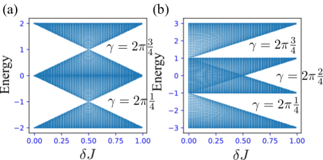
We calculate the single-particle spectrum of the system for two different parameter sets of and with periodic boundary condition. The results are shown in Fig. 14. In Fig. 11 (a) where we set and , at the first and second gap is closed and reopened for . When the system’s fermi-energy resides in the first gap, the filling is and there we observe Berry phase while with the fermi-energy in the second gap, the filling is and there we observe Berry phase .
We further show another different parameter set where and . The spectrum is shown in Fig. 11 (b). We observe that the first and third gap appear for while the second gap opens at . With the fermi-energy in the first gap, the filling is and there we observe Berry phase , with the fermi-energy in the second gap, the filling is , there we observe Berry phase and with the fermi-energy in the second gap, the filling is , there we observed Berry phase .
From these results, the free-fermion system also exhibits the various SPT phase protected by the symmetry.
References
- (1) T. Ozawa, H. M. Price, A. Amo, N. Goldman, M. Hafezi, L. Lu, M. C. Rechtsman, D. Schuster, J. Simon, O. Zilberberg, and I. Carusotto, Rev. Mod. Phys. 91, 015006 (2019).
- (2) M. Mancini, G. Pagano, G. Cappellini, L. Livi, M. Rider, J. Catani, C. Sias, P. Zoller, M. Inguscio, M. Dalmonte, and L. Fallani, Science 349, 1510 (2015).
- (3) B. K. Stuhl, H.-I. Lu, L. M. Aycock, D. Genkina, and I. B. Spielman, Science 349, 1514 (2015).
- (4) J. H. Kang, J. H. Han, and Y. Shin, Phys. Rev. Lett. 121, 150403 (2018).
- (5) J. H. Han, J.H. Kang, and Y. Shin, Phys. Rev. Lett. 122, 065303 (2019).
- (6) J. H. Kang, J. H. Han and Y. I. Shin, New J. Phys 22, 013023 (2020).
- (7) J. H. Han, D. Bae and Y. Shin Phys. Rev. A 105, 043306 (2022).
- (8) I. Bloch, J. Dalibard, and W. Zwerger, Rev. Mod. Phys. 80, 885 (2008).
- (9) C. Trefzger, C. Menotti, B. Capogrosso-Sansone, and M. Lewenstein, J. Phys. B 44, 193001 (2011).
- (10) S. Baier, M. J. Mark, D. Petter, K. Aikawa, L. Chomaz, Z. Cai, M. Baranov, P. Zoller, and F. Ferlaino, Science 352, 201 (2016).
- (11) F. Pollmann, E. Berg, A. M. Turner, and M. Oshikawa, Phys. Rev. B 85, 075125 (2012).
- (12) A. Altland and M. R. Zirnbauer, Phys. Rev. B 55, 1142 (1997).
- (13) A. Kitaev, AIP Conf. Proc. 1134, 22 (2009).
- (14) S. Ryu, A.P. Schnyder, A. Furusaki, and A.W.W. Ludwig, New J. Phys. 12, 065010 (2010).
- (15) X. Chen, Z. C. Gu, Z. X. Liu and X.G. Wen, Science 338, 6114, (2012).
- (16) X. Chen, Z. C. Gu, Z. X. Liu and X. G. Wen, Phys. Rev. B 87, 155114 (2013).
- (17) A. Mazurenko, C. S. Chiu, G. Ji, M. F. Parsons, M. Kanasz-Nagy, R. Schmidt, F. Grusdt, E. Demler, D. Greif, M. Greiner, Nature 545, 462-466 (2017).
- (18) Y. Hatsugai, Journal of the Physical Society of Japan 75, 123601 (2006).
- (19) T. Hirano, H. Katsura, and Y. Hatsugai, Phys. Rev. B 77, 094431 (2008)
- (20) I. Maruyama, T. Hirano, and Y. Hatsugai, Phys. Rev. B 79, 115107 (2009).
- (21) Y. Hatsugai and I. Maruyama, Epl 95, 20003 (2011).
- (22) N. Chepiga, F. Michaud, and F. Mila, Phys. Rev. B 88, 184418 (2013).
- (23) T. Kariyado and Y. Hatsugai, Phys. Rev. B 91, 214410 (2015).
- (24) I. Maruyama and S. Miyahara, J. Phys. Soc. Japan 87, 123703 (2018).
- (25) T. Kariyado, T. Morimoto, and Y. Hatsugai, Phys. Rev. Lett. 120, 247202 (2018).
- (26) T. Kawarabayashi, K. Ishii, and Y. Hatsugai, J. Phys. Soc. Japan 88, 045001 (2019).
- (27) T. Mizoguchi, H. Araki, and Y. Hatsugai, J. Phys. Soc. Japan 88, 104703 (2019).
- (28) H. Araki, T. Mizoguchi, and Y. Hatsugai, Phys. Rev. Research 2, 012009 (2020).
- (29) Y. Kuno and Y. Hatsugai, Phys. Rev. B 104, 125146 (2021).
- (30) Y. Otsuka, T. Yoshida, K. Kudo, S. Yunoki, and Y. Hatsugai, Sci. Rep. 11, 20270 (2021).
- (31) M. Bunney, T. Mizoguchi, Y. Hatsugai, and S. Rachel, Phys. Rev. B 105, 045113 (2022).
- (32) Y. Hatsugai and Y. Kuno, arXiv:2210.11646 (2022).
- (33) B. Paredes and I. Bloch, Phys .Rev A 77, 023603 (2008).
- (34) S. Nascimbène, Y.A. Chen, M. Atala, M. Aidelsburger, S. Trotzky, B. Paredes, and I. Bloch, Phys. Rev. Lett. 108, 205301 (2012).
- (35) M. Buser, C. Hubig, U. Schollwöck, L. Tarruell, and F. Heidrich-Meisner, Phys. Rev. A 102, 053314 (2020).
- (36) S. Greschner, M. Piraud, F. Heidrich-Meisner, I.P. McCulloch, U. Schollwöck, and T. Vekua, Phys. Rev. A 94, 063628 (2016).
- (37) T. Kariyado and Y. Hatsugai, Phys. Rev. B 90, 085132 (2014).
- (38) P. Weinberg and M. Bukov, SciPost Phys. 7, 20 (2019); 2, 003 (2017).
- (39) X. Deng and L. Santos, Phys. Rev. A 89, 033632 (2014).
- (40) Y. Kuno, K. Shimizu and I. Ichinose, New J. Phys. 19 123025 (2017).
- (41) J. Hauschild and F. Pollmann, SciPost Phys. Lect. Notes 5 (2018).
- (42) M. Oshikawa, M. Yamanaka, and I. Affleck, Phys. Rev. Lett. 78, 1984 (1997).
- (43) M. P. A. Fisher, P. B. Weichman, G. Grinstein, and D. S. Fisher, Phys. Rev. B 40, 546 (1989).
- (44) F. Grusdt, M. Höning, and M. Fleischhauer, Phys. Rev. Lett. 110, 260405 (2013).
- (45) S. Stumper and J. Okamoto, Phys. Rev. A 101, 63626 (2020).
- (46) Strictly, the edge states is not strict bonding state due to small , . However, our numerical result exhibits the edge state is much close to the bonding state. Thus, we call such a close state edge state in this subsection.
- (47) P. Sompet, S. Hirthe, D. Bourgund, T. Chalopin, J. Bibo, J. Koepsell, P. Bojović, R. Verresen, F. Pollmann, G. Salomon, C. Gross, T.A. Hilker, and I. Bloch, Nature 606, 484–488 (2022).
- (48) W. A. Benalcazar, B. A. Bernevig, and T. L. Hughes, Phys. Rev. B 96, 245115 (2017).
- (49) Y. You, J. Bibo, and F. Pollmann, Phys. Rev. Research 2, 033192 (2020).
- (50) D. González-Cuadra, Phys. Rev. B 105, L020403 (2022).