Far field broadband approximate cloaking for the Helmholtz equation with a Drude-Lorentz refractive index

Abstract

This paper concerns the analysis of a passive, broadband approximate cloaking scheme for the Helmholtz equation in ${\mathbb{R}}^{d}$ for $d=2$ or $d=3$. Using ideas from transformation optics, we construct an approximate cloak by “blowing up” a small ball of radius $\epsilon>0$ to one of radius $1$. In the anisotropic cloaking layer resulting from the “blow-up” change of variables, we incorporate a Drude-Lorentz-type model for the index of refraction, and we assume that the cloaked object is a soft (perfectly conducting) obstacle. We first show that (for any fixed $\epsilon$) there are no real transmission eigenvalues associated with the inhomogeneity representing the cloak, which implies that the cloaking devices we have created will not yield perfect cloaking at any frequency, even for a single incident time harmonic wave. Secondly, we establish estimates on the scattered field due to an arbitrary time harmonic incident wave. These estimates show that, as $\epsilon$ approaches $0$, the $L^{2}$-norm of the scattered field outside the cloak, and its far field pattern, approach $0$ uniformly over any bounded band of frequencies. In other words: our scheme leads to broadband approximate cloaking for arbitrary incident time harmonic waves.

1 Introduction

In this paper we analyze a passive, broadband approximate cloaking scheme for the Helmholtz equation in ${\mathbb{R}}^{d}$ for $d=2$ or $d=3$. Specifically, we are interested in making a bounded region approximately invisible to a far field observer and to probing by incident fields at arbitrary frequencies, independently of the material inside this region. Using ideas from transformation optics we achieve this by surrounding the region with a layer of an appropriate anisotropic material. By including a layer of extremely high conductivity adjacent to the region, we may without loss of generality assume that the region we want to cloak is “soft”, that is, supports a homogeneous Dirichlet boundary condition. The approach of cloaking by mapping, also known as transformation optics, has been popularized by Pendry, Schuring and Smith [28] and Leonhardt [22] for Maxwell’s equations. The basic idea is to make a singular change of variables which blows up a point (invisible to any probing incident wave) to a cloaked region. The same idea had previously been used by Greenleaf, Lassas and Uhlmann to create anisotropic objects that were invisible to EIT [15] (see also [14]). The singular nature of the perfect cloaks presents various difficulties: in practice this means they are hard to fabricate, and from the analysis point of view in some cases the rigorous definition of the corresponding electromagnetic fields is not obvious [12, 32, 33]. To avoid the use of singular materials in the cloak, regularized schemes have been suggested [19, 20, 29, 30]. The trade-off is that such schemes only lead to approximate cloaking. We refer the reader to [2, 8, 13, 16] for work on enhancement of approximate cloaks.

To design a passive approximate cloaking device, we blow up a small ball $B_{\epsilon}$ of radius $\epsilon>0$ (the regularization parameter) to the ball $B_{1}$ of radius one, which represents the cloaked region. To be more precise we actually map $B_{2}\setminus B_{\epsilon}$ onto $B_{2}\setminus B_{1}$, keeping fixed the outer boundary $\partial B_{2}$. $B_{2}\setminus B_{1}$ represents the cloak. As result of this change of variables one obtains an anisotropic layer in $B_{2}\setminus B_{1}$. We include a Drude-Lorentz-type term (see e.g. [18]) in the refractive index of the cloaking layer. This results in a frequency dependent and complex valued index of refraction which is consistent with causality. Since the cloaked region $B_{1}$ is “soft” we impose a zero Dirichlet boundary condition on the boundary $\partial B_{1}$. As mentioned earlier, this Dirichlet condition may be viewed as a limit of a highly conducting layer, and it thus may be interpreted as “hiding” the contents of $B_{1}$. A main focus of this paper is to establish estimates on the scattered field outside the cloak in terms of the small parameter $\epsilon>0$ and the probing frequencies. We remark that the choice of $B_{1}$ and $B_{2}\setminus{B_{1}}$ for the cloaked region and the cloak, respectively, is made for convenience and one can use more general domains in the change of variables. We also note that, in the context of approximate cloaking for the Helmholtz equation (the frequency domain wave equation), the Drude-Lorentz model was previously used by Nguyen and Vogelius in [27]. The Drude-Lorentz model takes into account the effect of the oscillations of free electrons on the electric permittivity by means of a simple harmonic oscillator model. When viewed in (complex) frequency domain, the refractive index associated with the Drude-Lorentz model may be extended analytically to the whole upper half plane. It is well-known that an immediate consequence of this is causality for the associated non-local time-domain wave equation, see [18, 31]. This property is most essential for the well-posedness (and the physical relevance) of this equation. Another well known consequence of this analyticity property are the so-called Kramers-Kronig relations between the real and the imaginary part of the refractive index (they are essentially related by Hilbert transforms). However, this fact is not explicitly used in our analysis.

We investigate two questions related to the scattering by the aforementioned cloak $B_{2}\setminus B_{1}$. The first one is whether, for a fixed $\epsilon>0$, there are wave numbers (proportional to frequencies) and incident fields for which the corresponding scattered field is zero, i.e., the cloak (and $B_{1}$) is perfectly invisible to this particular probing experiment. This question is related to the existence of real eigenvalues of the interior transmission eigenvalue problem defined on $B_{2}\setminus B_{1}$ [3], for which that part of the eigenfunction, which corresponds to the incident field, is extendable as a solution to the Helmholtz equation in all of ${\mathbb{R}}^{d}$ [6, 7]. In particular, such non-scattering wave numbers, for which perfect cloaking is achieved for a particular incident field, form a subset of the real transmission eigenvalues. We prove that, real transmission eigenvalues do not exist for the inhomogeneity presented by the cloak, i.e., for the anisotropic inhomogeneity $B_{2}\setminus B_{1}$ with the complex-valued frequency dependent Drude-Lorentz term and a homogeneous Dirichlet condition on the inner boundary $\partial B_{1}$. In addition, we show that all the (complex) transmission eigenvalues, that lie outside a precisely characterized compact set of the lower half plane, form a countable set with no finite accumulation points outside this compact set. Supported by some computational evidence, we conjecture that a sequence of complex transmission eigenvalues accumulate at a point (as well as at its symmetric counterpart) on the boundary of this compact set. These points have imaginary part equal to $-1/2$, but real parts that depend on the resonant frequency of the Drude-Lorentz term. A complete analysis of the transmission eigenvalue problem for inhomogeneities with such a Drude-Lorentz term is still open. This eigenvalue problem, in addition to being non-selfadjoint, is nonlinear since the Drude-Lorentz term involves the eigenvalue parameter in a non-linear fashion, and thus the known approaches do not apply [3]. If the Drude-Lorentz term is not present, the existence of an infinite set of real transmission eigenvalues accumulating at $+\infty$ for (anisotropic) inhomogeneities containing a Dirichlet obstacle is proven in [4, 5]. Secondly, although perfect cloaking is impossible at any frequency (even for a single incident wave) we prove that one can achieve approximate cloaking over any given finite band of wave numbers for sufficiently small $\epsilon>0$. In particular, we prove that provided the Drude-Lorentz resonant frequency $k_{\epsilon}$ is sufficiently large, more precisely $k_{\epsilon}^{2}>c_{*}\epsilon^{-3}$ for $d=3$, and $k_{\epsilon}^{2}>c_{*}|\ln\epsilon|/\epsilon$ for $d=2$, then for any fixed $R$ the $L^{2}$-norm of the scattered field in $B_{R}\setminus B_{2}$ is of order $\epsilon$ in ${\mathbb{R}}^{3}$ and of order $1/|\ln\epsilon|$ in ${\mathbb{R}}^{2}$, with a constant depending on the given band of wave numbers, $c_{*}$ and $R$. These estimates hold for a large class of incident waves, including plane waves and their superpositions (Herglotz waves). We note that point source waves with sources outside the cloak, as well as their superpositions would also be admissible. Furthermore, we prove that the far field pattern is uniformly $O(\epsilon)$ in ${\mathbb{R}}^{3}$ and $O(1/|\ln\epsilon|)$ in ${\mathbb{R}}^{2}$, with constants depending on the given band of wave numbers. These latter results are obtained by estimating the norm of the Lippmann-Schwinger volume integral over $B_{2}\setminus B_{1}$ and using scattering estimates adapted from [26]. We should mention that cloaking via change of variables for the Helmholtz equation at any frequency is investigated in [23, 24, 25, 26, 27], but in these papers the region is cloaked to an active source compactly supported in the exterior of the cloak. The scattering problem with incident field cannot be written in this framework. In fact, in that case the scattered field may be viewed as satisfying an inhomogeneous Helmholtz equation with a source given by the incident field, but this source is supported inside the cloak. Finally let us mention that perfect cloaking for the quasi-static Helmholtz equation (i.e., at zero frequency) with incident plane wave is investigated in [9]. One of the results proven there, namely that perfect cloaking is only possible at a discrete set of frequencies is entirely consistent with the fact that we in the present context show that there are no real transmission eigenvalues. Due to the lack of real transmission eigenvalues the lower bounds on cloaking effects provided in [9] are not very relevant here. In contrast our analysis demonstrates the possibility of broadband approximate cloaking in a certain (constitutive) regime.

2 Preliminaries

Let $B_{r}\subset\mathbb{R}^{d}$, $d=2$ or $d=3$ denote the open ball of radius $r>0$ centered at the origin and let $S_{r}=\partial B_{r}$. For a small parameter $\epsilon>0$ consider the following continuous and piecewise smooth mapping:

$$F(x)=\begin{cases}x,\hskip 72.26999pt&x\in\mathbb{R}^{d}\setminus B_{2}\\[3.61371pt] \displaystyle\left(\frac{2-2\epsilon}{2-\epsilon}+\frac{|x|}{2-\epsilon}\right)\frac{x}{|x|},\qquad&x\in B_{2}\setminus B_{\epsilon}\end{cases}$$ (2.1)

For simplicity of notation we will suppress the dependence of $F$ on the parameter $\epsilon$. Note that $F$ maps $B_{2}\setminus B_{\epsilon}$ onto $B_{2}\setminus B_{1}$, $S_{\epsilon}$ onto $S_{1}$, and that $F(x)=x$ on $S_{2}$. Now, we design a cloaking device, occupying $B_{2}\setminus B_{1}$, to approximately cloak the (soft) region $B_{1}$. We incorporate a Drude-Lorentz type term to account for a more physically relevant nonlinear dependence of the index of refraction on wavenumber. The constitutive material properties are thus given by

$$A_{c}(x);\ q_{c}(x,k)=\begin{cases}I;\ 1,\hskip 72.26999pt&x\in\mathbb{R}^{d}\setminus B_{2}\\[3.61371pt] F_{*}I;\ F_{*}1+\sigma_{\epsilon}(k),&x\in B_{2}\setminus B_{1},\end{cases}$$ (2.2)

where $I$ denotes the $d\times d$ identity matrix and $\sigma_{\epsilon}$ is the Drude-Lorentz term given by

$$\sigma_{\epsilon}(k)=\frac{1}{k_{\epsilon}^{2}-k^{2}-ik}~{},$$ (2.3)

cf. [18], page 331. Here $k_{\epsilon}>\frac{1}{2}$ represents the so-called resonant frequency of the Drude-Lorentz model. $F_{*}$ denotes the push-forward by the map $F$, defined by

$$F_{*}A(y)=\frac{DF(x)A(x)DF^{T}(x)}{|\det DF(x)|},\qquad F_{*}q(y)=\frac{q(x)}{|\det DF(x)|},\qquad x=F^{-1}(y)~{},$$

for a matrix-valued function $A$, and for a scalar function $q$, respectively. The definition of the push-forward is motivated by the following change of variables property, which can be proven by straightforward calculations (cf. [15, 19]).

Lemma 2.1.

Let $F$ be as defined in (2.1). Assume $A\in\left[L^{\infty}(B_{2}\setminus\overline{B_{\epsilon}})\right]^{d\times d}$ and $q\in L^{\infty}(B_{2}\setminus\overline{B_{\epsilon}})$. Then $u\in H^{1}(B_{2}\setminus\overline{B_{\epsilon}})\cap\{u=0\hbox{ on }S_{\epsilon}\}$ solves the equation

$$\mathrm{div}(A\nabla u)+qu=0,\qquad\text{in}\quad B_{2}\setminus\overline{B_{\epsilon}}~{},$$

iff $v=u\circ F^{-1}\in H^{1}(B_{2}\setminus\overline{B_{1}})\cap\{u=0\hbox{ on }S_{1}\}$ solves

$$\mathrm{div}(F_{*}A\nabla v)+F_{*}qu=0,\qquad\text{in}\quad B_{2}\setminus\overline{B_{1}}~{}.$$

The functions $u$ and $v$ satisfy the boundary relations

$$u=v,\quad\text{and}\quad A\nabla u\cdot\nu=F_{*}A\nabla v\cdot\nu,\qquad\text{on}\quad S_{2}~{},$$ (2.4)

where $\nu$ denotes the unit outward normal vector on $S_{2}$ and the equality of the conormal derivatives is understood in the sense of distributions in $H^{-\frac{1}{2}}(S_{2})$.

Furthermore

$$(F^{-1})_{*}\left[F_{*}A\right]=A~{},~{}\hbox{ and }~{}(F^{-1})_{*}\left[F_{*}q\right]=q~{}.$$

Let $u^{i}$ be an incident field at a given wave number $k>0$ (we suppress the dependence of $u^{i}$ on $k$ for the ease of notation), i.e.,

$$\Delta u^{i}+k^{2}u^{i}=0,\qquad\text{in}\quad\mathbb{R}^{d}.$$ (2.5)

Given the incident wave $u^{i}$ and the “cloaked” soft obstacle $B_{1}$, consider now the associated Helmholtz scattering problem. If $A_{c}$ and $q_{c}$ denote the constitutive material properties defined in (2.2), then the total field $u_{c}\in H^{1}_{loc}(\mathbb{R}^{d}\setminus\overline{B}_{1})$ is the unique solution to

$$\begin{cases}\mathrm{div}(A_{c}\nabla u_{c})+k^{2}q_{c}u_{c}=0,\qquad\qquad&\text{in}\quad\mathbb{R}^{d}\setminus\overline{B}_{1},\\ u_{c}=0,&\text{on}\quad S_{1}~{},\end{cases}$$ (2.6)

of the form

$$u_{c}=\begin{cases}u_{c}^{t},\qquad\qquad&\text{in}\quad B_{2}\setminus\overline{B}_{1}~{},\\ u^{i}+u_{c}^{s}&\text{in}\quad\mathbb{R}^{d}\setminus\overline{B}_{2}~{},\end{cases}$$ (2.7)

where $u_{c}^{t}$ is the transmitted field and $u_{c}^{s}$ is the scattered field, which satisfies the Sommerfeld radiation condition

$$\lim_{r\to\infty}r^{\frac{d-1}{2}}\left(\partial_{r}u_{c}^{s}-iku_{c}^{s}\right)=0,\quad\text{as}\quad r=|x|\to\infty~{},$$ (2.8)

uniformly in $\hat{x}=x/|x|$ (cf. [10] for more details about the scattering problem). As $u_{c}$ and its conormal derivative are continuous across $S_{2}$, the problem (2.6) can equivalently be written

$$\begin{cases}\Delta u_{c}^{s}+k^{2}u_{c}^{s}=0,\hskip 72.26999pt&\text{in}\quad\mathbb{R}^{d}\setminus\overline{B}_{2}\\[3.61371pt] u_{c}^{s}\ \text{satisfies the outgoing radiation condition}\\[3.61371pt] \nabla\cdot\left(A_{c}\nabla u_{c}^{t}\right)+k^{2}q_{c}u_{c}^{t}=0,&\text{in}\quad B_{2}\setminus\overline{B}_{1}\\[3.61371pt] \Delta u^{i}+k^{2}u^{i}=0,&\text{in}\quad\mathbb{R}^{d}\\[3.61371pt] u_{c}^{t}=u^{i}+u_{c}^{s},&\text{on}\quad S_{2}\\[3.61371pt] A_{c}\nabla u_{c}^{t}\cdot\nu=\partial_{\nu}u^{i}+\partial_{\nu}u_{c}^{s},&\text{on}\quad S_{2}\\[3.61371pt] u_{c}^{t}=0,&\text{on}\quad S_{1}.\end{cases}$$ (2.9)

As the scattered field $u_{c}^{s}$ satisfies the constant coefficient Helmholtz equation, it is in fact real analytic and admits the following asymptotic behavior as $r\to\infty$:

$$u_{c}^{s}(x)=\frac{e^{ikr}}{r^{\frac{d-1}{2}}}u^{\infty}(\hat{x})+O\left(r^{-\frac{d+1}{2}}\right),$$ (2.10)

where the function $u^{\infty}$, defined on $S_{1}$, is the so-called far field pattern of the scattered field $u_{c}^{s}$. It is well-known that the vanishing of $u^{\infty}$ on $S_{1}$, implies the vanishing of the scattered field $u_{c}^{s}$ in $\mathbb{R}^{d}\setminus\overline{B}_{2}$ (cf. Rellich’s Lemma in [10]). A non-trivial incident field $u^{i}$ and the wave number $k>0$ for which the corresponding far field pattern vanishes are referred to as non-scattering incident field and a non-scattering wave number, respectively. If we regard $u^{i}$ as a function defined in $B_{2}$, then from (2.9) it is clear that at a non-scattering wave number $k>0$, there exist non-trivial functions $w_{c}=u_{c}^{t}$ and $v=u^{i}$ defined in $B_{2}\setminus\overline{B}_{1}$ and $B_{2}$, respectively, such that

$$\begin{cases}\nabla\cdot\left(A_{c}\nabla w_{c}\right)+k^{2}q_{c}w_{c}=0,&\text{in}\quad B_{2}\setminus\overline{B}_{1}\\[3.61371pt] \Delta v+k^{2}v=0,&\text{in}\quad B_{2}\\[3.61371pt] w_{c}=v,&\text{on}\quad S_{2}\\[3.61371pt] A_{c}\nabla w_{c}\cdot\nu=\partial_{\nu}v,&\text{on}\quad S_{2}\\[3.61371pt] w_{c}=0,&\text{on}\quad S_{1}.\end{cases}$$ (2.11)

A wave number $k$ for which (2.11) admits a non-trivial solution is called an interior transmission eigenvalue with the corresponding eigenfunction $(w_{c},v)$. Thus, non-scattering wave numbers are necessarily real interior transmission eigenvalues [3]. Conversely, a real interior transmission eigenvalue $k>0$ is a non-scattering wave number if the eigenvector $v$ can be extended from $B_{2}$ to a solution of the Helmholtz equation in all of $\mathbb{R}^{d}$ [7, 6].

3 Main Results

For clarity and the reader’s convenience we now state the main results of our paper. The first theorem addresses the question whether our cloak provides a perfect cloaking of the region $B_{1}$ for even a single incident wave.

Theorem 3.1.

Consider the interior transmission eigenvalue problem (2.11).

1. There are no interior transmission eigenvalues in $\mathbb{R}\cup i\mathbb{R}$.

2. $k\in\mathbb{C}$ is an interior transmission eigenvalue if and only if so is $-\overline{k}$.

3. Assume $k_{\epsilon}>\frac{1}{\sqrt{2}}$, let $\kappa=\sqrt{k_{\epsilon}^{2}-\frac{1}{4}}-\frac{i}{2}$ and let $K$ be the shaded compact region in Figure 1. The region $K$ is symmetric about the imaginary axis, the slanted line segment of the boundary in the right half-plane has the equation $\mathfrak{Im}k=-\Re\mathfrak{e}k$, the curved arc joining $\kappa$ to $k_{\epsilon}$ is given by $\Re\mathfrak{e}k=\sqrt{(\mathfrak{Im}k)^{2}+\mathfrak{Im}k+k_{\epsilon}^{2}}$. Let $\mathcal{G}$ denote the open set $\mathcal{G}=\mathbb{C}\setminus K$. Then those interior transmission eigenvalues which lie inside $\mathcal{G}$ form a discrete set (i.e., an at most countable set with no limit points in $\mathcal{G}$).

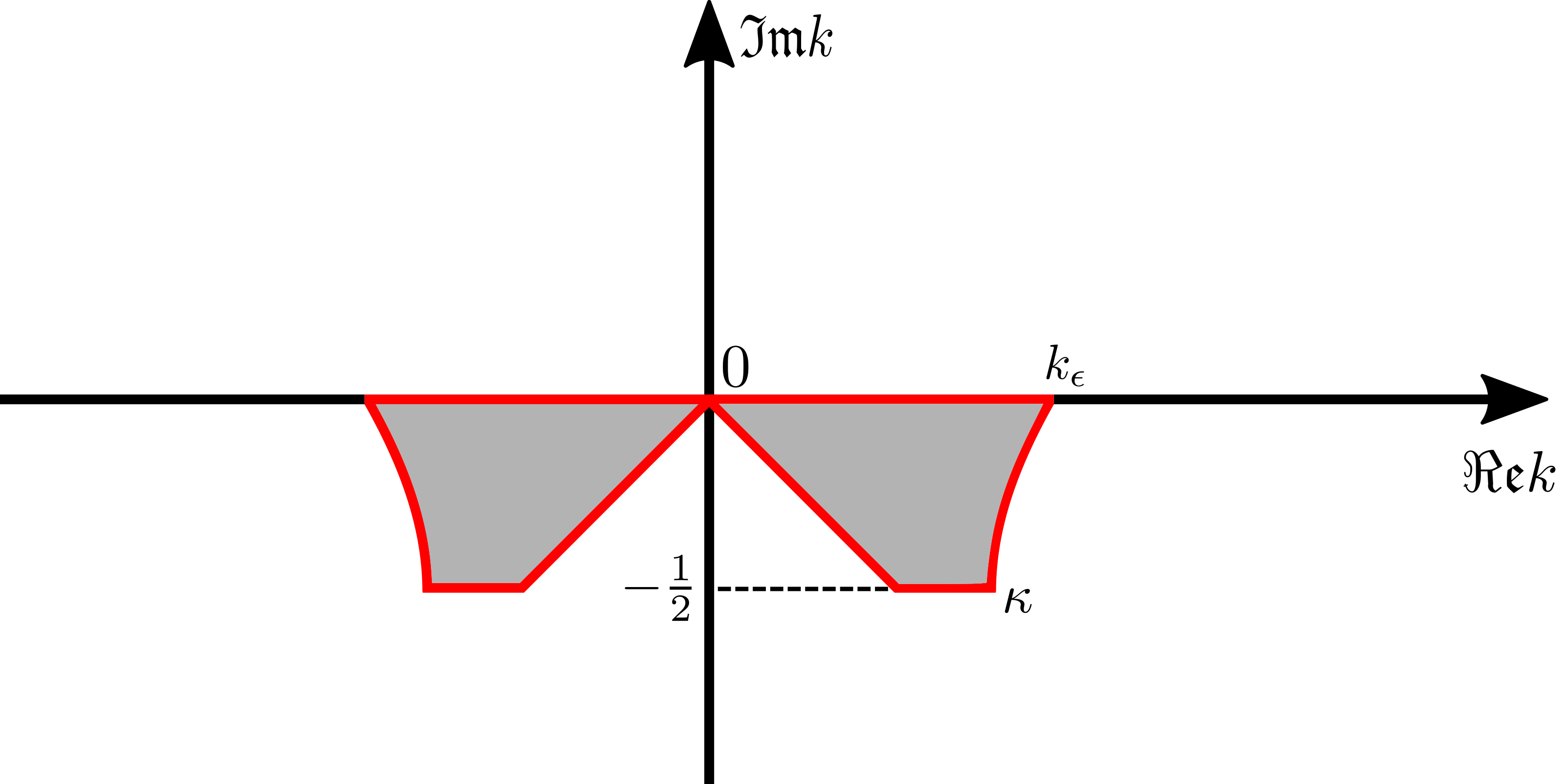
Figure 1: The shaded compact region $K$, outside of which the interior transmission eigenvalues of (2.11) form a discrete set.

Part $(i)$ of Theorem 3.1 will be proven in Section 4. As a consequence we conclude that perfect cloaking/non-scattering is impossible at any wave number $k>0$, since real transmission eigenvalues do not exist. Part $(ii)$ is an immediate consequence of the symmetry relation

$$\overline{\sigma_{\epsilon}(k)}=\sigma_{\epsilon}(-\overline{k})~{},\qquad\forall\ k\in\mathbb{C}~{}.$$

As a result $q_{c}(x,k)$ has the same symmetry property and $k$ is a transmission eigenvalue of (2.11) with eigenfunction $(w_{c},v)$, if and only if so is $-\overline{k}$ with eigenfunction $(\overline{w_{c}},\overline{v})$. The proof of part $(iii)$ will be given in the Appendix since the discreteness of complex eigenvalues is not central to the cloaking discussion. The value $\kappa$ is one of the poles of $\sigma_{\epsilon}(k)$ (the other one is $-\overline{\kappa}$). Numerical evidence, presented in Section 4.2, indicates that it is a limit point for the set of transmission eigenvalues of (2.11). Being bold, we venture

Conjecture 3.2.

(Finite accumulation point of transmission eigenvalues)

Let $\kappa$ be defined as in part $(iii)$ of Theorem 3.1. Then $\kappa$ is a limit point of transmission eigenvalues of (2.11).

We note that Theorem 3.1 asserts nothing about potential interior transmission eigenvalues in the set $K\setminus\mathbb{R}$. Their nature is a completely open problem.

Although perfect cloaking is impossible, we demonstrate that, under a suitable growth assumption on $k_{\epsilon}$, one can achieve approximate cloaking over any given finite band of wave numbers. We first state the main estimate on the scattered field including its explicit dependence on $k$ (and $\epsilon$). The broadband cloaking estimates follow as a corollary from this. We define

$$M_{\epsilon,k}=\|F_{*}^{-1}q_{c}-1\|_{L^{\infty}(B_{2}\setminus B_{\epsilon})}=\|F_{*}^{-1}\sigma_{\epsilon}(k)\|_{L^{\infty}(B_{2}\setminus B_{\epsilon})}~{},$$ (3.1)

where $F_{*}^{-1}$ denotes the push-forward by the map $F^{-1}$, and we set

$$a(k)=\begin{cases}1,\hskip 93.95122pt&d=3~{},\\ \min\{1+|\ln k|,k^{-\frac{1}{4}}\},&d=2~{}.\end{cases}$$ (3.2)

Theorem 3.3.

Let $R>2$ and $k_{0}>0$. Suppose $0<\epsilon k<k_{0}$ and suppose

$$\|u^{i}\|_{L^{\infty}(B_{\epsilon})}+\epsilon\|\nabla u^{i}\|_{L^{\infty}(B_{\epsilon})}\leq C~{}.$$ (3.3)

Let $u^{s}_{c}$ be the scattered field from (2.9). There exists a constant $c=c(k_{0},R)>0$ such that, if $k^{2}a(k)M_{\epsilon,k}<c$ then

$$\|u_{c}^{s}\|_{L^{2}(B_{R}\setminus B_{2})}\lesssim\epsilon+k^{2}a(k)M_{\epsilon,k}\|u^{i}\|_{L^{2}(B_{R})}~{},\qquad\qquad for\ d=3~{},$$ (3.4)

and

$$\|u_{c}^{s}\|_{L^{2}(B_{R}\setminus B_{2})}\lesssim\frac{|H_{0}^{(1)}(k)|}{|H_{0}^{(1)}(\epsilon k)|}+k^{2}a(k)M_{\epsilon,k}\left(1+\|u^{i}\|_{L^{2}(B_{R})}\right)~{},\qquad\qquad for\ d=2~{},$$ (3.5)

where the implicit constants in (3.4) and (3.5) depend only on $R,k_{0}$ and $C$.

Remark 3.4.

In the above theorem, $H_{0}^{(1)}$ denotes the Hankel function of the first kind of order $0$. We also adopt the following notation: for two positive quantities $A$ and $B$, we write $A\lesssim B$, if there exists a constant $d>0$ (independent of $A$ and $B$) such that $A\leq dB$.

Imposing a suitable lower bound on the resonant frequency $k_{\epsilon}$ with respect to $\epsilon$, the quantity $M_{\epsilon,k}$ (for bounded $k$) becomes of order $\epsilon$ for $d=3$, and of order $1/|\ln\epsilon|$ for $d=2$ (cf. (5.21)) and Theorem 3.3 implies the following result:

Theorem 3.5.

(Broadband approximate cloaking)

Let $R>2$, $k_{+}>k_{-}>0$, and set $\Gamma:=[k_{-},k_{+}]$. Assume that for some constant $c_{*}>0$,  $k_{\epsilon}^{2}>c_{*}\epsilon^{-3}$ for $d=3$, and $k_{\epsilon}^{2}>c_{*}|\ln\epsilon|/\epsilon$ for $d=2$. Furthermore, assume that the incident field $u^{i}$ satisfies

$$\|u^{i}\|_{L^{2}(B_{R})}\leq C_{R},\qquad\qquad\ \forall\ k\in\Gamma.$$ (3.6)

Let $u^{s}_{c}$ be the scattered field from(2.9). There exists a constant $c_{1}=c_{1}(k_{-},k_{+},R,c_{*})>0$ such that, for all $\epsilon<c_{1}$ and $k\in\Gamma$

$$\|u^{s}_{c}\|_{L^{2}(B_{R}\setminus B_{2})}\lesssim\begin{cases}\epsilon~{},\hskip 93.95122pt&d=3~{},\\[0.72229pt] 1/|\ln\epsilon|~{},&d=2~{},\end{cases}$$ (3.7)

where the implicit constant depends only on $k_{-},k_{+},R,c_{*}$ and $C_{R}$. Similarly, there exists a constant $c_{2}=c_{2}(k_{-},k_{+},c_{*})>0$, such that for all $\epsilon<c_{2}$,  $k\in\Gamma$, and $|\hat{x}|=1$

$$|u_{\infty}(\hat{x})|\lesssim\begin{cases}\epsilon~{},\hskip 93.95122pt&d=3~{},\\[0.72229pt] 1/|\ln\epsilon|~{},&d=2~{}.\end{cases}$$ (3.8)

where $u_{\infty}$ is the far field pattern defined in (2.10), and the implicit constant depends only on $k_{-},k_{+},c_{*}$ and $C_{5}$.

Remark 3.6.

1. The results of the above two theorems do not use the radial geometry in any essential way and carry over to the non-radial setting as well.

2. The assumption (3.6) (or (3.3)) is satisfied by incident plane waves as well as by their superpositions, the so-called Herglotz waves $u^{i}:=u_{g}$ given by

   $$u_{g}(x)=\int_{|\hat{y}|=1}g(\hat{y})e^{ikx\cdot\hat{y}}\,ds_{\hat{y}}~{},\qquad g\in L^{2}(S_{1})~{}.$$

   It is also satisfied by radiating point sources (outside of $B_{2}$) and their appropriate superpositions.

4 Transmission eigenvalues

In this section we study the interior transmission eigenvalue problem. We first eliminate the anisotropy $A_{c}$ in the formulation (2.11) by using a change of variables to arrive at a new interior transmission eigenvalue problem, which has the same eigenvalues as (2.11). Then we reformulate the resulting problem in terms of a fourth order PDE, following [4] (see also [3]). Using this new formulation we prove part $(i)$ of Theorem 3.1. Furthermore, in Section 4.2 we present numerical evidence supporting Conjecture 3.2 in two dimension.

4.1 The variational formulation

In the interior transmission eigenvalue problem (2.11) let us change the variables in $w_{c}$, while leaving $v$ unchanged. Namely, let

$$w=w_{c}\circ F,$$

where $F$ is defined by (2.1). Using the properties of the map $F$ (namely that $F(x)=x$ on $S_{2}$, $F$ maps $S_{\epsilon}$ onto $S_{1}$ and $F_{*}^{-1}A_{c}=F_{*}^{-1}F_{*}I=I$ in $B_{2}\setminus\overline{B}_{1}$) along with Lemma 2.1, we obtain that $w,v$ solve the following transmission problem:

$$\begin{cases}\Delta w+k^{2}qw=0~{},\qquad\qquad&\text{in}\ B_{2}\setminus\overline{B}_{\epsilon}\\ \Delta v+k^{2}v=0~{},&\text{in}\ B_{2}\\ w=v~{},&\text{on}\ S_{2}\\ \partial_{\nu}w=\partial_{\nu}v&\text{on}\ S_{2}\\ w=0~{},&\text{on}\ S_{\epsilon}\end{cases}$$ (4.1)

where

$$q(x,k)=F^{-1}_{*}q_{c}(x,k)=F^{-1}_{*}\left[F_{*}1+\sigma_{\epsilon}(k)\right]=1+\sigma_{\epsilon}(k)|\det DF(x)|~{},\qquad\qquad x\in B_{2}\setminus\overline{B}_{\epsilon}~{}.$$

Let us introduce the notation

$${\mathcal{O}}:=B_{2}\setminus\overline{B}_{\epsilon}.$$

It is clear that $k\in\mathbb{C}$ is a transmission eigenvalue for (2.11) with eigenfunction $(w_{c},v)$, if and only if, it is a transmission eigenvalue for (4.1) with eigenfunction $(w=w_{c}\circ F,v)$. Thus (2.11) and (4.1) have the same set of transmission eigenvalues. We recall that the weak solution of (4.1) is a pair of functions $w\in L^{2}_{\Delta}({\mathcal{O}})$ and $v\in L^{2}_{\Delta}(B_{2})$ that satisfy the PDEs of (4.1) in the sense of distributions, such that $w=0$ on $S_{\epsilon}$ and $u:=w-v\in H^{1}_{\Delta}({\mathcal{O}})$ satisfies the boundary conditions $u=\partial_{\nu}u=0$ on $S_{2}$.

Remark 4.1.

1. We note that the trace (on $S_{\epsilon}$) of a function $w\in L^{2}_{\Delta}({\mathcal{O}})$ makes sense as an element of $H^{-\frac{1}{2}}(S_{\epsilon})$ by duality, using the identity

   $$\left<w,\tau\right>_{H^{-1/2},H^{1/2}}=\int_{{\mathcal{O}}}(w\Delta\varphi-\varphi\Delta w)\,dx~{},$$

   where $\varphi\in H^{2}({\mathcal{O}})$ is such that $\varphi=0$ in a neighborhood of $S_{2}$, and $\varphi=0$ and $\partial\varphi/\partial\nu=\tau$ on $S_{\epsilon}$ .

2. Similarly we note that for a function $u\in H^{1}_{\Delta}({\mathcal{O}})$ the normal derivative $\partial_{\nu}u$ (on $S_{2}$) makes sense as an element of $H^{-\frac{1}{2}}(S_{2})$ by duality, using the formula

   $$\left<\partial_{\nu}u,\psi\right>_{H^{-1/2},H^{1/2}}=\int_{{\mathcal{O}}}\left(\Delta u\varphi+\nabla u\nabla\varphi\right)\,dx~{},$$

   where $\varphi\in H^{1}({\mathcal{O}})$ is such that $\varphi=0$ on $S_{\epsilon}$, and $\varphi=\psi$ on $S_{2}$.

We can reformulate (4.1) as a fourth order problem. Indeed, given a weak solution $w,v$ of (4.1), let us set

$$u=\begin{cases}w-v,\qquad&\text{in}\ {\mathcal{O}}\\ -v,&\text{in}\ B_{\epsilon},\end{cases}$$ (4.2)

It is clear that

$$\Delta u+k^{2}qu=k^{2}(1-q)v,\qquad\qquad\text{in}\ {\mathcal{O}}.$$ (4.3)

Dividing both sides of the above equation by $1-q$ (note that $1-q=-\sigma_{\epsilon}(k)|\det DF|\neq 0$ in ${\mathcal{O}}$) and applying the operator $\Delta+k^{2}$ we can eliminate $v$ and obtain a fourth order equation for $u$. The boundary condition on $w$ implies that $u$ is continuous across $S_{\epsilon}$. Next, since $v$ solves the Helmholtz equation in $B_{2}$, $v$ and its normal derivative $\partial_{\nu}v$ are continuous across $S_{\epsilon}$. We can rewrite these continuity conditions in terms of $u$ using (4.2) and (4.3). Thus, we obtain that $u$ (weakly) solves the problem

$$\begin{cases}\displaystyle(\Delta+k^{2})\frac{1}{1-q}(\Delta+k^{2}q)u=0,\qquad\qquad&\text{in}\ {\mathcal{O}}\\[6.50403pt] \Delta u+k^{2}u=0,&\text{in}\ B_{\epsilon}\\ u=\partial_{\nu}u=0,&\text{on}\ S_{2}\\ u^{+}=u^{-},&\text{on}\ S_{\epsilon}\\ \displaystyle\left[\frac{1}{1-q}(\Delta+k^{2}q)u\right]^{+}=-k^{2}u^{-},&\text{on}\ S_{\epsilon}\\[10.84006pt] \displaystyle\partial_{\nu}^{+}\left[\frac{1}{1-q}(\Delta+k^{2}q)u\right]=-k^{2}\partial_{\nu}^{-}u,&\text{on}\ S_{\epsilon}.\end{cases}$$ (4.4)

Note that as $v\in L^{2}(B_{2})$ solves the Helmholtz equation, by local elliptic regularity $v\in H^{1}(B_{\epsilon})$. But as $u$ is continuous across $S_{\epsilon}$, we conclude that $u\in H^{1}(B_{2})\cap H^{1}_{\Delta}({\mathcal{O}})$. Incorporating the boundary conditions on $S_{2}$ we introduce the Hilbert space of functions

$$X=\left\{u\in H^{1}(B_{2}):\Delta u\in L^{2}({\mathcal{O}})\ \text{and}\ u=\partial_{\nu}u=0\ \text{on}\ S_{2}\right\},$$ (4.5)

where $\partial_{\nu}u\in H^{-\frac{1}{2}}(S_{2})$, and is defined as described in the earlier remark. Thus, given a non-trivial weak solution $w,v$ of (4.1), the function $u\in X$, given by (4.2), is a non-trivial weak solution of (4.4). Conversely, if $u\in X$ is a non-trivial weak solution of (4.4), then

$$v=\begin{cases}\displaystyle\frac{1}{1-q}\left(\Delta+k^{2}q\right)u,\quad&\text{in}\ {\mathcal{O}}\\ -k^{2}u,&\text{in}\ B_{\epsilon}\end{cases}\qquad\text{and}\qquad w=k^{2}u+v,\quad\text{in}\ {\mathcal{O}},$$ (4.6)

satisfy $w\in L^{2}({\mathcal{O}}),\ v\in L^{2}(B_{2})$ and $w-v\in H^{1}_{\Delta}({\mathcal{O}})$ and yield a non-trivial weak solution of (4.1). Integration by parts easily yields a variational formulation of (4.4), namely : find $u\in X$ such that

$$\int_{{\mathcal{O}}}\frac{1}{1-q}\left(\Delta u+k^{2}u\right)\left(\Delta\overline{\varphi}+k^{2}\overline{\varphi}\right)dx$$ (4.7)

$$\hskip 60.0pt-k^{4}\int_{B_{2}}u\overline{\varphi}dx+k^{2}\int_{B_{2}}\nabla u\cdot\nabla\overline{\varphi}dx=0,\qquad\qquad\forall\varphi\in X.$$

Before excluding the existence of real and purely imaginary transmission eigenvalues we need the following formulas for the map $F$:

Lemma 4.2.

Let $F$ be given by (2.1), and set $\hat{x}=x/|x|$, then

$$DF(x)=\begin{cases}I,\hskip 180.67499pt&\text{in}\ \mathbb{R}^{d}\setminus B_{2}\\[3.61371pt] \dfrac{1}{2-\epsilon}\left\{I+\frac{2-2\epsilon}{|x|}\left(I-\hat{x}\otimes\hat{x}\right)\right\},&\text{in}\ B_{2}\setminus B_{\epsilon}\\[7.22743pt] I/\epsilon,&\text{in}\ B_{\epsilon},\end{cases}$$

where $I$ is the $d\times d$ identity matrix and for any two vectors $a,b\in\mathbb{R}^{d}$, $a\otimes b$ denotes the matrix whose $(i,j)$-th element is $a_{i}b_{j}$. In particular,

$$\det DF(x)=\begin{cases}1\hskip 108.405pt&\text{in}\ \mathbb{R}^{d}\setminus B_{2}\\[3.61371pt] \displaystyle\frac{(2-2\epsilon+|x|)^{d-1}}{(2-\epsilon)^{d}|x|^{d-1}}&\text{in}\ B_{2}\setminus B_{\epsilon}\\[7.22743pt] 1/\epsilon^{d}&\text{in}\ B_{\epsilon}.\end{cases}$$ (4.8)

Proof.

The formulas for $DF(x)$ inside $B_{\epsilon}$ and outside of $B_{2}$ are trivial. In the region $B_{2}\setminus B_{\epsilon}$ it is a direct consequence of the identity

$$D\hat{x}=\frac{1}{|x|}\left(I-\hat{x}\otimes\hat{x}\right)$$

Finally, using the identity $\det(I+a\otimes b)=1+a\cdot b$ for any two vectors $a,b\in\mathbb{R}^{d}$, we find that for $x\in B_{2}\setminus B_{\epsilon}$

$$\det DF(x)=\frac{1}{(2-\epsilon)^{d}}\left[\frac{2-2\epsilon}{|x|}+1\right]^{d-1},$$

which concludes the proof. ∎

Lemma 4.3.

There are no non-trivial solutions to (2.11) for $k\in\mathbb{R}\cup i\mathbb{R}$, i.e., there are no transmission eigenvalues for (2.11) in $\mathbb{R}\cup i\mathbb{R}$.

Proof.

First suppose $k=i\tau$ with $\tau\in\mathbb{R}$ is a transmission eigenvalue. The above discussion shows that the problem (4.4) has a non-trivial solution $u\in X$ for this value of $k$. Using the variational formulation (4.7) with $\varphi=u$ we get

$$0=\int_{{\mathcal{O}}}\frac{1}{q-1}\left|\Delta u-\tau^{2}u\right|^{2}+\tau^{4}\int_{B_{2}}|u|^{2}dx+\tau^{2}\int_{B_{2}}|\nabla u|^{2}dx~{}.$$ (4.9)

Note that

$$q(x,i\tau)-1=\sigma_{\epsilon}(i\tau)|\det DF(x)|=\frac{1}{k_{\epsilon}^{2}+\tau^{2}+\tau}\frac{(2-2\epsilon+|x|)^{d-1}}{(2-\epsilon)^{d}|x|^{d-1}}~{},\qquad\qquad x\in{\mathcal{O}}~{}.$$

If $\tau\geq 0$ the above quantity is obviously positive. For $\tau<0$, it is still positive due to the assumption $2k_{\epsilon}>1$. Thus $q(x,i\tau)-1>0$ for all $\tau\in\mathbb{R}$ and $x\in{\mathcal{O}}$. For $\tau\neq 0$ we now conclude from (4.9) that $u=0$ in $B_{2}$, contradicting the non-triviality of $u$ for $\tau\neq 0$. For $\tau=0$ we conclude from (4.9) that $\Delta u=0$ in $\mathcal{O}$. The Cauchy boundary conditions on $S_{2}$ now imply that $u=0$ in $\mathcal{O}$, and the continuity of $u$ across $S_{\epsilon}$ in combination with the fact that $\Delta u=0$ in $B_{\epsilon}$ yields that $u=0$ in all of $B_{2}$, contradicting the non-triviality of $u$ also for $\tau=0$.

Assume now that $k\in\mathbb{R}\setminus\{0\}$ is a transmission eigenvalue; again let $\varphi=u$ in the variational formulation (4.7) and take the imaginary part of the resulting equation to conclude that

$$0=\int_{{\mathcal{O}}}\mathfrak{Im}\left(\frac{1}{q-1}\right)\left|\Delta u+k^{2}u\right|^{2}dx=\frac{k}{|k_{\epsilon}^{2}-k^{2}-ik|^{2}}\int_{{\mathcal{O}}}\frac{(2-2\epsilon+|x|)^{d-1}}{(2-\epsilon)^{d}|x|^{d-1}}\left|\Delta u+k^{2}u\right|^{2}dx~{}.$$

Therefore $\Delta u+k^{2}u=0$ in ${\mathcal{O}}$. Using the boundary conditions $u=\partial_{\nu}u=0$ on $S_{2}$, we conclude that $u=0$ in ${\mathcal{O}}$. Since $k\neq 0$ also conclude from the boundary conditions of (4.4) that $u^{-}=\partial_{\nu}^{-}u=0$ on $S_{\epsilon}$. The fact that $\Delta u+k^{2}u=0$ in $B_{\epsilon}$ now implies that $u=0$ in $B_{\epsilon}$, and thus $u=0$ in all of $B^{2}$. This contradicts the non-triviality of $u$. ∎

4.2 Numerical evidence of finite accumulation points of transmission eigenvalues

In this section we assume that $d=2$ and consider the transmission eigenvalue problem after change of variables, i.e., the problem (4.1). In polar coordinates $(r,\theta)$ we can expand the functions $v$ and $w$ as follows:

$$v(r,\theta)=\sum_{n\in\mathbb{Z}}\gamma_{n}J_{n}\left(kr\right)e^{in\theta},\qquad\qquad w(r,\theta)=\sum_{n\in\mathbb{Z}}\left[\alpha_{n}{\mathcal{A}}_{n}(r)+\beta_{n}{\mathcal{B}}_{n}(r)\right]e^{in\theta}$$ (4.10)

where $\alpha_{n},\beta_{n},\gamma_{n}$ are complex constants, $J_{n}$ is the Bessel function of order $n$ and ${\mathcal{A}}_{n},{\mathcal{B}}_{n}$ (which also depend on $k$ and $\epsilon$) are linearly independent solutions of

$$r^{2}R^{\prime\prime}+rR^{\prime}+\left[k^{2}r^{2}+k^{2}\sigma_{\epsilon}(k)\frac{r(r+2-2\epsilon)}{(2-\epsilon)^{2}}-n^{2}\right]R=0~{}.$$

The boundary conditions of (4.1) can be rewritten as

$$\begin{cases}\alpha_{n}{\mathcal{A}}_{n}(2)+\beta_{n}{\mathcal{B}}_{n}(2)&=\gamma_{n}J_{n}(2k)\\[3.61371pt] \alpha_{n}A_{n}^{\prime}(2)+\beta_{n}{\mathcal{B}}_{n}^{\prime}(2)&=\gamma_{n}kJ_{n}^{\prime}(2k)\\[3.61371pt] \alpha_{n}{\mathcal{A}}_{n}(\epsilon)+\beta_{n}{\mathcal{B}}_{n}(\epsilon)&=0~{}.\end{cases}$$

To obtain a nontrivial solution $(v,w)$ (i.e., to ensure that $k$ is an interior transmission eigenvalue) we need that there exists some $n\in\mathbb{Z}$ such that

$$f(n,k):=\det\mathcal{M}=0~{},$$

where

$$\mathcal{M}=\begin{pmatrix}{\mathcal{A}}_{n}(2)&{\mathcal{B}}_{n}(2)&-J_{n}(2k)\\ A_{n}^{\prime}(2)&{\mathcal{B}}_{n}^{\prime}(2)&-kJ_{n}^{\prime}(2k)\\ {\mathcal{A}}_{n}(\epsilon)&{\mathcal{B}}_{n}(\epsilon)&0\end{pmatrix}~{}.$$

The functions $A_{n},{\mathcal{B}}_{n}$ can be expressed in terms of the Whittaker functions as follows:

$${\mathcal{A}}_{n}(r)=\frac{1}{\sqrt{r}}M_{\lambda_{\epsilon}(k),|n|}\left(\frac{2ik\sqrt{\sigma_{\epsilon}(k)+(2-\epsilon)^{2}}}{\epsilon-2}r\right),$$ (4.11)

where

$$\lambda_{\epsilon}(k)=\frac{ik\sigma_{\epsilon}(k)(1-\epsilon)}{(2-\epsilon)\sqrt{\sigma_{\epsilon}(k)+(2-\epsilon)^{2}}}~{},$$ (4.12)

and ${\mathcal{B}}_{n}$ is given by the same formula except with $W_{\lambda_{\epsilon}(k),|n|}$ in place of $M_{\lambda_{\epsilon}(k),|n|}$. The Whittaker functions $M_{\lambda,n}(x)$ and $W_{\lambda,n}(x)$ (for any non-negative integer $n$) are linearly independent solutions of the equation [1]

$$y^{\prime\prime}+\left(-\frac{1}{4}+\frac{\lambda}{x}+\frac{\frac{1}{4}-n^{2}}{x^{2}}\right)y=0~{}.$$

Let us take $k_{\epsilon}=\frac{1}{\epsilon}$ and $\epsilon=\frac{1}{2}$, then

$$\kappa=\sqrt{k_{\epsilon}^{2}-\tfrac{1}{4}}-\frac{i}{2}\approx 1.936-i0.5$$

We show some numerical evidence that $\kappa$ is a limit point of transmission eigenvalues. We conjecture that for each $n=1,2,...$ there exists $k_{n}\in\mathbb{C}\setminus\{\kappa\}$ such that $f(n,k_{n})=0$ and $k_{n}\to\kappa$ as $n\to\infty$. In other words, $\kappa$ is a limit point of the transmission eigenvalues $\{k_{n}\}$.

For each of the values $n=1$, $n=7$, and $n=12$, we present two plots of the functions $\Re\mathfrak{e}f(n,x+i\tau)$ and $\mathfrak{Im}f(n,x+i\tau)$ as functions of $x$, corresponding to two different values of $\tau$. The two values of $\tau$ are chosen to be close to $\mathfrak{Im}\kappa=-0.5$, and such that they exhibit two different configurations: one for which the intersection point of $\Re\mathfrak{e}f$ and $\mathfrak{Im}f$ is below the horizontal axis, and one for which it is above the horizontal axis. This shows that for some intermediate value of $\tau$ both $\Re\mathfrak{e}f$ and $\mathfrak{Im}f$ vanish. It is reasonable to expect that this common vanishing occurs at a point $x$ near the $x$ values of the two intersection points. One notes that as $n$ increases the $x$ values of the two intersection points get closer to $1.936-i0.5$ Computations for larger values of $n$ were consistent with this.

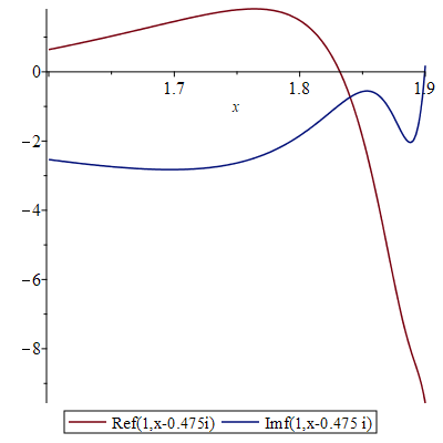
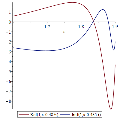
Figure 2: Plots of real and imaginary parts of $f(n,x+i\tau)$ for $n=1$ and two different values of $\tau$ indicating where their intersection point crosses the horizontal axis.

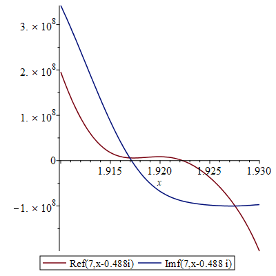
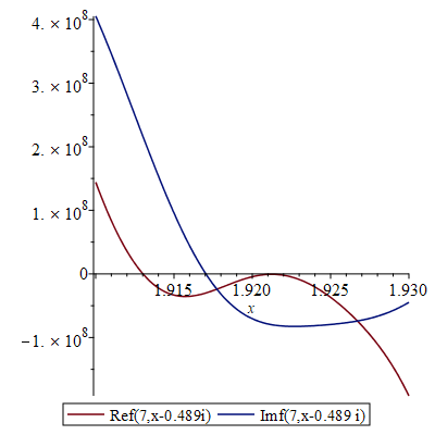
Figure 3: Plots of real and imaginary parts of $f(n,x+i\tau)$ for $n=7$ and two different values of $\tau$ indicating where their intersection point crosses the horizontal axis.

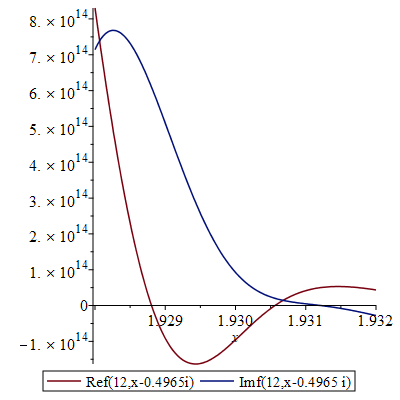
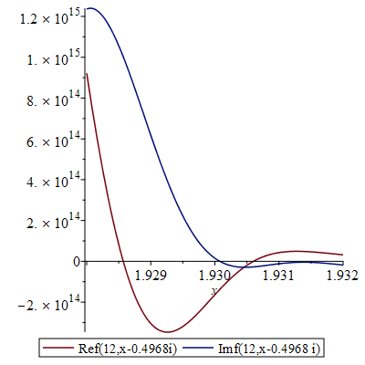
Figure 4: Plots of real and imaginary parts of $f(n,x+i\tau)$ for $n=12$ and two different values of $\tau$ indicating where their intersection point crosses the horizontal axis.

5 The scattering estimates

In this section we prove Theorems 3.3 and 3.5. The first observation is that the anisotropy in (2.9) can be eliminated, if we change the variables in the transmitted filed $u_{c}^{t}$, but leave the incident and scattered fields unchanged. Namely, let

$$u^{s}=u^{s}_{c},\qquad u^{t}=u_{c}^{t}\circ F,$$ (5.1)

where $F$ is given by (2.1), then $u^{t}$ is defined in $B_{2}\setminus\overline{B}_{\epsilon}$.

Invoking Lemma 2.1 and using the facts that $F=Id$ on $S_{2}$, $F$ maps $S_{\epsilon}$ onto $S_{1}$ and that $F^{-1}_{*}A_{c}=I$, we see that (2.9) can be equivalently rewritten as

$$\begin{cases}\Delta u^{s}+k^{2}u^{s}=0~{},\hskip 72.26999pt&\text{in}\quad\mathbb{R}^{d}\setminus\overline{B}_{2}\\[3.61371pt] u^{s}\ \text{satisfies the outgoing radiation condition}\\[3.61371pt] \Delta u^{t}+k^{2}qu^{t}=0~{},&\text{in}\quad B_{2}\setminus\overline{B}_{\epsilon}\\[3.61371pt] \Delta u^{i}+k^{2}u^{i}=0~{},&\text{in}\quad\mathbb{R}^{d}\\[3.61371pt] u^{t}=u^{i}+u^{s}~{},&\text{on}\quad S_{2}\\[3.61371pt] \partial_{\nu}u^{t}=\partial_{\nu}u^{i}+\partial_{\nu}u^{s}~{},&\text{on}\quad S_{2}\\[3.61371pt] u^{t}=0,&\text{on}\quad S_{\epsilon}~{},\end{cases}$$ (5.2)

where

$$q(x,k)=F^{-1}_{*}q_{c}(x,k)=\begin{cases}1~{},\hskip 108.405pt&\text{in}\quad\mathbb{R}^{d}\setminus B_{2}\\[7.22743pt] \displaystyle 1+\sigma_{\epsilon}(k)|\det DF(x)|,&\text{in}\quad B_{2}\setminus B_{\epsilon}~{}.\end{cases}$$ (5.3)

Introducing

$$u=\begin{cases}u^{t}~{},\qquad\qquad&\text{in}\quad B_{2}\setminus\overline{B}_{\epsilon}\\ u^{i}+u^{s},&\text{in}\quad\mathbb{R}^{d}\setminus B_{2}~{},\end{cases}$$ (5.4)

the problem (5.2) can be rewritten as find $u\in H^{1}_{loc}(\mathbb{R}^{d}\setminus\overline{B}_{\epsilon})$

$$\begin{cases}\Delta u+k^{2}qu=0~{},\hskip 72.26999pt&\text{in}\quad\mathbb{R}^{d}\setminus\overline{B}_{\epsilon}\\[3.61371pt] \Delta u^{i}+k^{2}u^{i}=0~{},&\text{in}\quad\mathbb{R}^{d}\\[3.61371pt] u=0~{},&\text{on}\quad S_{\epsilon}\\[3.61371pt] u-u^{i}\ \ \text{satisfies the outgoing radiation condition}.\end{cases}$$ (5.5)

Here we used that the boundary conditions on $S_{2}$ from (5.2) simply become $[\![u]\!]=[\![\partial_{\nu}u]\!]=0$ on $S_{2}$, i.e., $u$ and its normal derivative are continuous across $S_{2}$.

5.1 The Lippmann-Schwinger equation

Consider the fundamental solution of the Helmholtz equation in free space: for any $x\neq y$

$$\Phi_{k}(x,y)=\begin{cases}\dfrac{e^{ik|x-y|}}{4\pi|x-y|}~{},\qquad\quad&d=3~{},\\[10.84006pt] \dfrac{i}{4}H_{0}^{(1)}(k|x-y|)~{},&d=2~{}.\end{cases}$$ (5.6)

We incorporate the homogeneous Dirichlet boundary condition of (5.5) into the fundamental solution, i.e., we let $\Phi_{k}^{0}$ be the Green’s function for the Helmholtz equation in the region $\mathbb{R}^{d}\setminus\overline{B}_{\epsilon}$ with the Dirichlet boundary condition in $S_{\epsilon}$. For any fixed $y\in\mathbb{R}^{d}\setminus\overline{B}_{\epsilon}$ $\Phi_{k}^{0}(x,y)$ satisfies

$$\begin{cases}\Delta_{x}\Phi^{0}_{k}(x,y)+k^{2}\Phi^{0}_{k}(x,y)=-\delta_{y}~{},\hskip 72.26999pt&\quad x\in\mathbb{R}^{d}\setminus\overline{B}_{\epsilon}\\[3.61371pt] \Phi^{0}_{k}(x,y)=0~{},&\quad x\in S_{\epsilon}\\[3.61371pt] \Phi^{0}_{k}(\cdot,y)\ \ \text{satisfies the outgoing radiation condition}~{}.\end{cases}$$ (5.7)

Clearly we can write

$$\Phi^{0}_{k}(x,y)=\Phi_{k}(x,y)+\Psi_{k}(x,y)~{},$$

where the function $\Psi_{k}(\cdot,y)$ is the unique solution to the following exterior Dirichlet boundary value problem for the Helmholtz equation

$$\begin{cases}\Delta_{x}\Psi_{k}(x,y)+k^{2}\Psi_{k}(x,y)=0~{},\qquad\qquad&x\in\mathbb{R}^{d}\setminus\overline{B}_{\epsilon}\\ \Psi_{k}(x,y)=-\Phi_{k}(x,y)~{},&x\in\ S_{\epsilon}\\[3.61371pt] \Psi_{k}(\cdot,y)\ \ \text{satisfies the outgoing radiation condition}~{}.\end{cases}$$ (5.8)

Note that the boundary data $-\Phi_{k}(x,y)$ is smooth, hence the function $\Psi_{k}(x,y)$ is smooth for $x\in\mathbb{R}^{d}\setminus B_{\epsilon}$ and for any fixed $y$ as above. Next, let us introduce the volume integral operator

$$Tu(x)=k^{2}\int_{B_{2}\setminus\overline{B}_{\epsilon}}(q(y,k)-1)u(y)\Phi_{k}^{0}(x,y)dy.$$ (5.9)

Then the solution $u$ of (5.5) satisfies the integral equation

$$u-Tu=u^{i}+u^{is},$$ (5.10)

where $u^{is}$ is the scattered field from the ball $B_{\epsilon}$ due to the incident field $u^{i}$, i.e., it is the unique solution of

$$\begin{cases}\Delta u^{is}+k^{2}u^{is}=0,\qquad\qquad&\text{in}\ \mathbb{R}^{d}\setminus\overline{B}_{\epsilon}\\ u^{is}=-u^{i},&\text{on}\ S_{\epsilon}\\[3.61371pt] u^{is}\ \ \text{satisfies the outgoing radiation condition}.\end{cases}$$ (5.11)

The equation (5.10) is known as the Lippmann-Schwinger equation for the scattering problem (5.5) written in terms of the Green’s function $\Phi_{k}^{0}$. It can be derived the same way as done for example in [10](without Dirichlet boundary conditions and using the kernel $\Phi_{k}$). In Lemma 5.1 (see also (5.23) and (5.24) ) we prove that for any fixed interval of wave numbers $[k_{-},k_{+}]$, $0<k_{-}<k_{+}<\infty$, and any fixed $R>2$ there exists an $\epsilon_{0}>0$ (depending on $k_{+}$ and $R$) such that

$$\|T\|_{L^{2}(B_{R}\setminus B_{\epsilon})\to L^{2}(B_{R}\setminus B_{\epsilon})}\leq\frac{1}{2},$$ (5.12)

for any $k\in[k_{-},k_{+}]$, and $\epsilon<\epsilon_{0}$. Therefore the operator $I-T$ is invertible on $L^{2}(B_{R}\setminus B_{\epsilon})$ and the integral equation (5.10) has a unique solution $u_{R}\in L^{2}(B_{R}\setminus B_{\epsilon})$. Furthermore $u_{R}=u|_{B_{R}\setminus B_{\epsilon}}$ where $u$ is the solution of (5.5). This follows from the fact that $u|_{B_{R}\setminus B_{\epsilon}}$ is in $L^{2}(B_{R}\setminus B_{\epsilon})$ and as already noted satisfies the integral equation (5.10). It now follows immediately from (5.10), and the fact that the domain of integration for the operator $T$ is $B_{2}\setminus B_{\epsilon}$, that the solution to (5.5) is given by

$$u=Tu_{R}+u^{i}+u^{is}$$

in all of ${\mathbb{R}}^{d}\setminus B_{\epsilon}$. Note that due to the mapping properties of the volume potential $Tu_{R}$ is in $H^{1}_{loc}({\mathbb{R}}^{d}\setminus B_{\epsilon})$. The above argument shows that solving (5.5) is equivalent to solving the Lippmann-Schwinger equation (5.10) on $B_{R}\setminus B_{\epsilon}$ (for any bounded set of wave numbers $[k_{-},k_{+}]$ and $\epsilon$ sufficiently small).

5.2 Proof of Theorems 3.3 and 3.5

The main ingredients of the proofs of Theorems 3.3 and 3.5 are $\epsilon$-explicit estimates for the scattered field $u^{is}$ and the operator $T$ in appropriate Sobolev spaces. We state these estimates in the two lemmata below, however, for clarity of exposition their proofs are postponed to subsequent sections (see Section 5.3 and Section 5.4, respectively).

Lemma 5.1.

Let $T$ be defined by (5.9), and let $M_{\epsilon,k}$ and $a(k)$ be defined by (3.1) and (3.2), respectively. Suppose $R>1$, $k_{0}>0$, and $0<\epsilon k<k_{0}$. Then for any $u\in L^{2}(B_{2}\setminus B_{\epsilon})$

$$\|Tu\|_{L^{2}(B_{R}\setminus B_{\epsilon})}\lesssim k^{2}a(k)M_{\epsilon,k}\|u\|_{L^{2}(B_{2}\setminus B_{\epsilon})}~{},$$

where the implicit constant depends only on $R$ and $k_{0}$.

Lemma 5.2.

Let $u^{is}$ be defined by (5.11), let $R>1$, and $k_{0}>0$. Assume $0<\epsilon k<k_{0}$ and that $u^{i}$ satisfies (3.3), then

$$\|u^{is}\|_{L^{2}(B_{R}\setminus B_{1})}\lesssim\begin{cases}\epsilon~{},\hskip 50.58878pt&d=3~{},\\[7.22743pt] \dfrac{|H_{0}^{(1)}(k)|}{|H_{0}^{(1)}(\epsilon k)|}~{},&d=2~{},\end{cases}$$

and

$$\|u^{is}\|_{L^{2}(B_{R}\setminus B_{\epsilon})}\lesssim\epsilon^{d-2}~{},$$

where the implicit constants depends only on $R,k_{0}$ and $C$ (the constant from the inequality (3.3) for the incident field $u^{i}$).

With the help of the above lemmata we now prove the following scattering estimate:

Theorem 5.3.

Let $M_{\epsilon,k}$ and $a(k)$ be defined by (3.1) and (3.2), respectively. Suppose $R>2$, $k_{0}>0$, and $0<\epsilon k<k_{0}$, and suppose $u^{i}$ satisfies (3.3). Let $u$ be be the solution to (5.5). There exists a constant $c=c(k_{0},R)>0$ such that, if $k^{2}a(k)M_{\epsilon,k}<c$, then

$$\|u-u^{i}\|_{L^{2}(B_{R}\setminus B_{\epsilon})}\lesssim\epsilon^{d-2}+k^{2}a(k)M_{\epsilon,k}\|u^{i}\|_{L^{2}(B_{R})}~{},\qquad\qquad for\ d=2,3~{}~{},$$ (5.13)

and

$$\|u-u^{i}\|_{L^{2}(B_{R}\setminus B_{1})}\lesssim\frac{|H_{0}^{(1)}(k)|}{|H_{0}^{(1)}(\epsilon k)|}+k^{2}a(k)M_{\epsilon,k}\left(1+\|u^{i}\|_{L^{2}(B_{R})}\right)~{},\qquad\qquad for\ d=2~{},$$ (5.14)

where the implicit constants depend only on $R,k_{0}$ and $C$ (the constant from the inequality (3.3)).

Remark 5.4.

As an immediate corollary we obtain Theorem 3.3, because $u-u^{i}=u^{s}=u^{s}_{c}$ outside $B_{2}$.

Proof.

Consider the Lippmann-Schwinger equation (5.10) in the space $L^{2}(B_{R}\setminus B_{\epsilon})$. Lemma 5.1 implies that there exists a constant $C_{1}=C_{1}(k_{0},R)>0$, such that

$$\|T\|_{L^{2}(B_{R}\setminus B_{\epsilon})\to L^{2}(B_{R}\setminus B_{\epsilon})}\leq C_{1}k^{2}a(k)M_{\epsilon,k}=:r$$

Assume that $r<\frac{1}{2}$, or equivalently $k^{2}a(k)M_{\epsilon,k}<\frac{1}{2C_{1}}=:c$. Then the operator $I-T$ is invertible on $L^{2}(B_{R}\setminus B_{\epsilon})$ and using (5.10) and the Neumann series expansion we obtain

$$u=(I-T)^{-1}(u^{i}+u^{is})=u^{i}+u^{is}+\sum_{n=1}^{\infty}T^{n}(u^{i}+u^{is}).$$

Upon summation of the geometric series, the above equation implies the bound

$$\begin{split}\|u-u^{i}\|_{L^{2}(B_{R}\setminus B_{\epsilon})}&\leq\|u^{is}\|_{L^{2}(B_{R}\setminus B_{\epsilon})}+\frac{r}{1-r}\|u^{i}+u^{is}\|_{L^{2}(B_{R}\setminus B_{\epsilon})}\\ &\leq\|u^{is}\|_{L^{2}(B_{R}\setminus B_{\epsilon})}+2r\left(\|u^{i}\|_{L^{2}(B_{R})}+\|u^{is}\|_{L^{2}(B_{R}\setminus B_{\epsilon})}\right)\\ &\lesssim\|u^{is}\|_{L^{2}(B_{R}\setminus B_{\epsilon})}+r\|u^{i}\|_{L^{2}(B_{R})}\\ &\lesssim\epsilon^{d-2}+r\|u^{i}\|_{L^{2}(B_{R})},\end{split}$$

where in the last step we used Lemma 5.2. This concludes the proof of the inequality (5.13).

To prove (5.14), we take $d=2$. From the Lippmann-Schwinger equation $u-u^{i}=u^{is}+Tu$, and hence, using Lemma 5.2 we have ,

$$\|u-u^{i}\|_{L^{2}(B_{R}\setminus B_{1})}\leq\|u^{is}\|_{L^{2}(B_{R}\setminus B_{1})}+\|Tu\|_{L^{2}(B_{R}\setminus B_{\epsilon})}\lesssim\frac{|H_{0}^{(1)}(k)|}{|H_{0}^{(1)}(\epsilon k)|}+r\|u\|_{L^{2}(B_{R}\setminus B_{\epsilon})}.$$

From (5.13) with $d=2$ we have

$$\begin{split}\|u\|_{L^{2}(B_{R}\setminus B_{\epsilon})}&\leq\|u^{i}\|_{L^{2}(B_{R})}+\|u-u^{i}\|_{L^{2}(B_{R}\setminus B_{\epsilon})}\lesssim\|u^{i}\|_{L^{2}(B_{R})}+1+k^{2}a(k)M_{\epsilon,k}\|u^{i}\|_{L^{2}(B_{R})}\\ &\lesssim 1+\|u^{i}\|_{L^{2}(B_{R})},\end{split}$$

where in the last step we used the assumption that $k^{2}a(k)M_{\epsilon,k}<c$. A combination of the last two estimates and insertion of $r=C_{1}k^{2}a(k)M_{\epsilon,k}$ leads to (5.14).

∎

Before proceeding to the proof of Theorem 3.5, we first estimate the far field pattern $u_{\infty}$, given by (2.10), in terms of the $L^{2}(B_{5}\setminus B_{2})$-norm of the scattered field $u^{s}$, given by (5.1) and (2.9).

In the following, by using the term “an absolute implicit constant”, we signify that, the inequality in question holds with a positive constant independent of the involved parameters.

Lemma 5.5.

With an absolute implicit constant, for any $|\hat{x}|=1$ and $k>0$,

$$|u_{\infty}(\hat{x})|\lesssim(1+k^{3})\|u^{s}\|_{L^{2}(B_{5}\setminus B_{2})}\begin{cases}1~{},\qquad&d=3~{},\\[7.22743pt] k^{-\frac{1}{2}}~{},&d=2~{}.\end{cases}$$ (5.15)

Proof.

The far field pattern has the following representation [10]:

$$u_{\infty}(\hat{x})=\mathcal{I}\cdot\begin{cases}\dfrac{1}{4\pi}~{},\qquad&d=3~{},\\[7.22743pt] \dfrac{e^{i\frac{\pi}{4}}}{\sqrt{8\pi k}}~{},&d=2~{},\end{cases}$$

where

$$\mathcal{I}=\int_{S_{4}}\left(u^{s}(y)\partial_{\nu_{y}}e^{-ik\hat{x}\cdot y}-\partial_{\nu}u^{s}(y)e^{-ik\hat{x}\cdot y}\right)ds(y)~{},$$

and $S_{4}$ is the $d-1$-sphere of radius $4$ centered at the origin (note that one could use any $d-1$ manifold circumscribing $B_{2}$ in its interior). Using Hölder’s inequality and the duality $H^{-\frac{1}{2}}\subset L^{2}\subset H^{\frac{1}{2}}$ with the pivot space $L^{2}$, we can bound

$$\begin{split}|\mathcal{I}|\lesssim&k\|u^{s}\|_{L^{2}(S_{4})}+\|e^{-ik\hat{x}\cdot y}\|_{H^{\frac{1}{2}}(S_{4})}\|\partial_{\nu}u^{s}\|_{H^{-\frac{1}{2}}(S_{4})}\\[3.61371pt] \lesssim&k\|u^{s}\|_{H^{1}(B_{4}\setminus B_{3})}+\|e^{-ik\hat{x}\cdot y}\|_{H^{1}(B_{4}\setminus B_{3})}\|\partial_{\nu}u^{s}\|_{H^{-\frac{1}{2}}(S_{4})}\\[3.61371pt] \lesssim&k\|u^{s}\|_{H^{1}(B_{4}\setminus B_{3})}+(1+k)\|\partial_{\nu}u^{s}\|_{H^{-\frac{1}{2}}(S_{4})}~{},\end{split}$$

where in the second step we used trace estimates. Next we bound the $H^{-\frac{1}{2}}$-norm of $\partial_{\nu}u^{s}$. Given any $\phi\in H^{\frac{1}{2}}(S_{4})$, consider its extension to $B_{4}\setminus\overline{B}_{3}$ via a bounded right inverse of the trace operator:

$$\begin{cases}w_{\phi}\in H^{1}(B_{4}\setminus\overline{B}_{3})\\ w_{\phi}=0~{},\qquad&\text{on}\ S_{3}~{},\\ w_{\phi}=\phi~{},&\text{on}\ S_{4}~{}.\end{cases}$$ (5.16)

As this defines a bounded operator from $H^{\frac{1}{2}}(S_{3}\cup S_{4})$ to $H^{1}(B_{4}\setminus\overline{B}_{3})$, we have that with an absolute implicit constant

$$\|w_{\phi}\|_{H^{1}(B_{4}\setminus B_{3})}\lesssim\|\phi\|_{H^{\frac{1}{2}}(S_{4})}~{}.$$ (5.17)

Now using the fact that $u^{s}$ satisfies the Helmholtz equation in $B_{4}\setminus\overline{B}_{3}$, we obtain

$$\langle\partial_{\nu}u^{s},\phi\rangle=\int_{B_{4}\setminus B_{3}}\nabla u^{s}\cdot\nabla w_{\phi}+w_{\phi}\Delta u^{s}dy=\int_{B_{4}\setminus B_{3}}\nabla u^{s}\cdot\nabla w_{\phi}-k^{2}w_{\phi}u^{s}dy~{},$$

where $\langle\cdot,\cdot\rangle$ denotes the dual pairing between $H^{-\frac{1}{2}}(S_{4})$ and $H^{\frac{1}{2}}(S_{4})$. Using the Hölder’s inequality and (5.17) we arrive at

$$|\langle\partial_{\nu}u^{s},\phi\rangle|\lesssim\|\phi\|_{H^{\frac{1}{2}}(S_{4})}\left(\|\nabla u^{s}\|_{L^{2}(B_{4}\setminus B_{3})}+k^{2}\|u^{s}\|_{L^{2}(B_{4}\setminus B_{3})}\right)~{},$$

which readily implies

$$\|\partial_{\nu}u^{s}\|_{H^{-\frac{1}{2}}(S_{4})}\lesssim\|\nabla u^{s}\|_{L^{2}(B_{4}\setminus B_{3})}+k^{2}\|u^{s}\|_{L^{2}(B_{4}\setminus B_{3})}~{}.$$

Using that $k+k^{2}+k^{3}\lesssim k+k^{3}$, we obtain the bound

$$|\mathcal{I}|\lesssim(k+k^{3})\|u^{s}\|_{L^{2}(B_{4}\setminus B_{3})}+(1+k)\|\nabla u^{s}\|_{L^{2}(B_{4}\setminus B_{3})}.$$ (5.18)

It remains to bound the $L^{2}$-norm of $\nabla u^{s}$, which can be done via the $L^{2}$-norm of $u^{s}$ over a larger domain by introducing a cut-off function and using the equation that $u^{s}$ satisfies. Indeed, let $0\leq\psi\leq 1$ be a cut-off function such that $\text{supp}\ \psi\subset B_{5}\setminus\overline{B}_{2}$,  $\psi\equiv 1$ on $B_{4}\setminus\overline{B}_{3}$ and $|\nabla\psi|\leq C$ on $B_{5}\setminus\overline{B}_{2}$, with an absolute constant $C>0$. Since

$$\Delta u^{s}+k^{2}u^{s}=0,\qquad\qquad\text{in}\ B_{5}\setminus\overline{B}_{2}~{},$$

multiplication by $\psi^{2}\overline{u^{s}}$ and integration by parts leads to

$$\begin{split}\int_{B_{5}\setminus B_{2}}|\nabla u^{s}|^{2}\psi^{2}dy&=k^{2}\int_{B_{5}\setminus B_{2}}|u^{s}|^{2}\psi^{2}dy-2\int_{B_{5}\setminus B_{2}}\psi\nabla u^{s}\cdot\overline{u^{s}}\nabla\psi dy\\ &\leq k^{2}\int_{B_{5}\setminus B_{2}}|u^{s}|^{2}\psi^{2}dy+\frac{1}{2}\int_{B_{5}\setminus B_{2}}|\nabla u^{s}|^{2}\psi^{2}dy+2\int_{B_{5}\setminus B_{2}}|u^{s}|^{2}|\nabla\psi|^{2}dy~{},\end{split}$$

which implies

$$\frac{1}{2}\int_{B_{5}\setminus B_{2}}|\nabla u^{s}|^{2}\psi^{2}dy\leq(k^{2}+2C^{2})\int_{B_{5}\setminus B_{2}}|u^{s}|^{2}dy~{}.$$

Consequently,

$$\|\nabla u^{s}\|_{L^{2}(B_{4}\setminus B_{3})}\lesssim(1+k)\|u^{s}\|_{L^{2}(B_{5}\setminus B_{2})}~{}.$$

Combining with (5.18) we obtain

$$|\mathcal{I}|\lesssim(k+k^{3})\|u^{s}\|_{L^{2}(B_{5}\setminus B_{2})}+(1+k)^{2}\|u^{s}\|_{L^{2}(B_{5}\setminus B_{2})}\lesssim(1+k^{3})\|u^{s}\|_{L^{2}(B_{5}\setminus B_{2})}~{},$$ (5.19)

which concludes the proof. ∎

We are ready to establish the following broadband approximate cloaking estimates:

Theorem 5.6.

Let $R>2$ and $k_{+}>k_{-}>0$, and set $\Gamma=[k_{-},k_{+}]$. Assume that for some constant $c_{*}>0$,  $k_{\epsilon}^{2}>c_{*}\epsilon^{-3}$ for $d=3$, and $k_{\epsilon}^{2}>c_{*}|\ln\epsilon|/\epsilon$ for $d=2$. Assume further that $u^{i}$ satisfies the estimate (3.6). Let $u$ be the solution to (5.5) with $q$ given by (5.3). There exists a constant $c_{1}=c_{1}(k_{-},k_{+},R,c_{*})>0$ such that, for all $\epsilon<c_{1}$ and $k\in\Gamma$

$$\|u-u^{i}\|_{L^{2}(B_{R}\setminus B_{1})}\lesssim\begin{cases}\epsilon~{},\hskip 93.95122pt&d=3~{},\\[0.72229pt] 1/|\ln\epsilon|~{},&d=2~{},\end{cases}$$

where the implicit constant depends only on $k_{-},k_{+},R,c_{*}$ and $C_{R}$ (the constants from (3.6)). Furthermore, there exists a constant $c_{2}=c_{2}(k_{-},k_{+},c_{*})>0$, such that for all $\epsilon<c_{2}$,  $k\in\Gamma$ and $|\hat{x}|=1$,

$$|u_{\infty}(\hat{x})|\lesssim\begin{cases}\epsilon~{},\hskip 93.95122pt&d=3~{},\\[0.72229pt] 1/|\ln\epsilon|~{},&d=2~{},\end{cases}$$

where the implicit constant depends only on $k_{-},k_{+},c_{*}$ and $C_{5}$.

Remark 5.7.

1. Since $u-u^{i}=u^{s}_{c}$ outside of $B_{2}$ Theorem 3.5 follows as an immediate corollary of the above result.

2. For $d=3$ the following proof can be easily modified to show we can bound $u-u^{i}$ up to the inner boundary $S_{\epsilon}$, i.e.,

   $$\|u-u^{i}\|_{L^{2}(B_{R}\setminus B_{\epsilon})}\lesssim\epsilon~{}.$$

Proof.

We note that since $u^{i}$ is a solution to $\Delta u^{i}+k^{2}u^{i}=0$ in all of ${\mathbb{R}}^{d}$, it follows by interior elliptic regularity estimates that for $k\in\Gamma$, $\|u^{i}\|_{L^{\infty}(B_{1})}+\|\nabla u^{i}\|_{L^{\infty}(B_{1})}\leq C\|u^{i}\|_{L^{2}(B_{2})}$, with a constant that only depends on $k_{+}$. Due to (3.6) we thus conclude that $u^{i}$, $k\in\Gamma$, satisfies the condition (3.3) as well (for $\epsilon<1$) with a constant that only depends on $C_{2}$ and $k_{+}$.

We proceed to estimate $M_{\epsilon,k}$. In view of (3.1), (5.3) and Lemma 4.2,

$$M_{\epsilon,k}=|\sigma_{\epsilon}(k)|\|\det DF\|_{L^{\infty}(B_{2}\setminus B_{\epsilon})}=\frac{|\sigma_{\epsilon}(k)|}{(2-\epsilon)^{d}}\sup_{r\in(\epsilon,2)}\left(1+\frac{2-2\epsilon}{r}\right)^{d-1}=\frac{|\sigma_{\epsilon}(k)|}{(2-\epsilon)\epsilon^{d-1}}.$$

Assume that $\epsilon<1$ is so small that

$$k_{\epsilon}^{2}\geq\max\left\{k_{+}^{2},2(k_{+}^{2}-k_{+})\right\},$$ (5.20)

then for any $k\in[0,k_{+}]$

$$|\sigma_{\epsilon}(k)|\leq\frac{\sqrt{2}}{|k_{\epsilon}^{2}-k^{2}|+k}=\frac{\sqrt{2}}{k_{\epsilon}^{2}-k^{2}+k},$$

where in the last step we used that $k_{\epsilon}^{2}\geq k^{2}_{+}$. The function $k\mapsto k_{\epsilon}^{2}-k^{2}+k$ is positive and increasing on $[0,\frac{1}{2}]$, and it is positive and decreasing on $[\frac{1}{2},k_{+}]$ (if $k_{+}>\frac{1}{2}$). Thus it follows that

$$k_{\epsilon}^{2}-k^{2}+k\geq\min\{k_{\epsilon}^{2},k_{\epsilon}^{2}-k_{+}^{2}+k_{+}\}\geq\frac{k_{\epsilon}^{2}}{2}~{}~{}\hbox{ for }k\in[0,k_{+}]~{},$$

where in the second inequality we have used that $k_{\epsilon}^{2}\geq 2(k_{+}^{2}-k_{+})$. As a consequence

$$\max_{k\in\Gamma}|\sigma_{\epsilon}(k)|\leq\frac{2\sqrt{2}}{k_{\epsilon}^{2}}\leq\frac{2\sqrt{2}}{c_{*}}\begin{cases}\epsilon^{3},\qquad\qquad&d=3,\\ \epsilon/|\ln\epsilon|,&d=2.\end{cases}$$

We now conclude that there exist positive constants $c_{0},C_{0}$ depending only on $c_{*}$ and $k_{+}$, such that

$$\max_{k\in\Gamma}M_{\epsilon,k}\leq C_{0}\begin{cases}\epsilon,\qquad\qquad&d=3,\\ 1/|\ln\epsilon|,&d=2,\end{cases}\qquad\qquad\forall\ \epsilon\leq c_{0}~{}.$$ (5.21)

Let us further assume $\epsilon<1/k_{+}$ so that $0<\epsilon k<1$ for $k\in\Gamma$. By Theorem 5.3 there exists a constant $c=c(R)>0$ such that if $k^{2}a(k)M_{\epsilon,k}<c$ (and $k$ is in $\Gamma$) then

$$\|u-u^{i}\|_{L^{2}(B_{R}\setminus B_{1})}$$

$$\hskip 5.0pt\lesssim\begin{cases}\epsilon+k^{2}M_{\epsilon,k}\|u^{i}\|_{L^{2}(B_{R})}\hskip 50.58878pt&\text{for}\ d=3~{},\\[3.61371pt] \displaystyle\frac{|H_{0}^{(1)}(k)|}{|H_{0}^{(1)}(\epsilon k)|}+k^{2}M_{\epsilon,k}\min\{1+|\ln k|,k^{-\frac{1}{4}}\}\left(1+\|u^{i}\|_{L^{2}(B_{R})}\right)&\text{for}\ d=2~{}.\end{cases}$$ (5.22)

Consider first the case $d=3$. If we assume that $\epsilon<c/C_{0}k_{+}^{2}$, then

$$\max_{k\in\Gamma}k^{2}M_{\epsilon,k}\leq k_{+}^{2}C_{0}\epsilon<c~{},$$ (5.23)

and consequently (5.2) can be applied for all $k\in\Gamma$. Using the hypothesis (3.6) and (5.21) we conclude that for $\epsilon$ small enough

$$\max_{k\in\Gamma}\|u-u^{i}\|_{L^{2}(B_{R}\setminus B_{1})}\lesssim\epsilon\qquad\qquad\text{for}\ d=3~{},$$

where the implicit constant depends only on $k_{+},R,c_{*}$ and $C_{R}$.

Let us now consider $d=2$. The function $a(k)=\min\{1+|\ln k|,k^{-\frac{1}{4}}\}$ is decreasing, therefore, assuming that $\epsilon<e^{-C_{0}k_{+}^{2}a(k_{-})/c}$ we have

$$\max_{k\in\Gamma}k^{2}a(k)M_{\epsilon,k}\leq\frac{C_{0}}{|\ln\epsilon|}k_{+}^{2}a(k_{-})<c~{}.$$ (5.24)

Similarly, as before we conclude that, for $k\in\Gamma$,

$$\|u-u^{i}\|_{L^{2}(B_{R}\setminus B_{1})}\lesssim\frac{|H_{0}^{(1)}(k)|}{|H_{0}^{(1)}(\epsilon k)|}+\frac{1}{|\ln\epsilon|}~{}.$$

The function $|H_{0}^{(1)}(t)|$ is decreasing and $H_{0}^{(1)}(t)\sim\frac{2}{i\pi}|\ln t|$ as $t\to 0$ (cf. [21]). Hence we have the following basic estimates: $|H_{0}^{(1)}(k)|\leq|H_{0}^{(1)}(k_{-})|$ and

$$|H_{0}^{(1)}(t)|\gtrsim|\ln t|,\qquad\qquad\forall\ t\in(0,\tfrac{1}{2}).$$

These readily imply the inequality

$$\|u-u^{i}\|_{L^{2}(B_{R}\setminus B_{1})}\lesssim\frac{1}{|\ln(\epsilon k)|}+\frac{1}{|\ln\epsilon|}.$$

Since by assumption $\epsilon k_{+}<1$ we get

$$\min_{k\in\Gamma}|\ln(\epsilon k)|=|\ln(\epsilon k_{+})|\geq\frac{1}{2}|\ln\epsilon|~{},$$

where the last inequality holds, provided $\epsilon<1/k_{+}^{2}$. Putting everything together we conclude that for $\epsilon$ sufficiently small

$$\max_{k\in\Gamma}\|u-u^{i}\|_{L^{2}(B_{R}\setminus B_{1})}\lesssim\frac{1}{|\ln\epsilon|}~{}.$$

The corresponding estimates for the far field pattern readily follow from Lemma 5.5.

∎

5.3 Scattering from a small obstacle: Proof of Lemma 5.2

In this section we show that Lemma 5.2 is a direct consequence of the following result due to Nguyen and Vogelius [26] (see also [23]):

Lemma 5.8.

Let $D\subset B_{1}\subset\mathbb{R}^{d}$ be a smooth open subset with $\mathbb{R}^{d}\setminus\overline{D}$ connected. Let $f\in H^{\frac{1}{2}}(\partial D)$, $k_{0}>0$ and $0<k<k_{0}$. Let $u$ be the outward radiating solution to the problem

$$\begin{cases}\Delta u+k^{2}u=0,\qquad\qquad&\text{in}\ \mathbb{R}^{d}\setminus\overline{D}~{},\\ u=f&\text{on}\ \partial D~{}.\end{cases}$$

Then for any $\beta\geq 1$

$$\|u\|_{H^{1}(B_{\beta}\setminus D)}\lesssim\begin{cases}\beta^{\frac{1}{2}}\|f\|_{H^{\frac{1}{2}}(\partial D)}~{},\qquad&d=3~{},\\ \beta\|f\|_{H^{\frac{1}{2}}(\partial D)}~{},&d=2~{},\end{cases}$$ (5.25)

where the implicit constant depends only on $k_{0}$ and $D$ but is independent of $\beta$ and $k$. Furthermore, for $R>1,\beta\geq 1$

$$\|u\|_{L^{2}(B_{R\beta}\setminus B_{\beta})}\lesssim\beta\frac{|H_{0}^{(1)}(\beta k)|}{|H_{0}^{(1)}(k)|}\|f\|_{H^{\frac{1}{2}}(\partial D)}~{},\qquad\qquad d=2~{},$$ (5.26)

where the implicit constant depends only on $k_{0},D$, and $R$ but is independent of $\beta$ and $k$.

Remark 5.9.

The estimate (5.25) for the $L^{2}$-norm of $u$ and (5.26), in the case $R=2$, is proven in Lemma 3 of [26] under the assumption that $k_{0}$ is sufficiently small (see also the beginning of the proof of Lemma 4). The subsequent Remark 4 of [26] explains that these estimates hold without any smallness assumption on $k_{0}$. The extension of (5.26) to any $R>1$ is immediate. Finally, the extension from an $L^{2}$ estimate of $u$ to an $H^{1}$ estimate, as in (5.25), is guaranteed by Lemma 4 of [26].

As a straightforward consequence of Lemma 5.8 (with $D=B_{\frac{1}{2}}\subset B_{1}$) we obtain the following corollary.

Corollary 5.10.

(Scattering from a small ball)

Let $\epsilon<\frac{1}{2}$, $R>1,k_{0}>0$ with $0<2\epsilon k<k_{0}$. Let $f\in H^{\frac{1}{2}}(S_{\epsilon})$ and $u$ be the outward radiating solution of the problem

$$\begin{cases}\Delta u+k^{2}u=0,\qquad\qquad&\text{in}\ \mathbb{R}^{d}\setminus\overline{B}_{\epsilon}\\ u=f&\text{on}\ S_{\epsilon}\end{cases}$$

Let $R>1$ and set $f_{\epsilon}=f(2\epsilon\cdot)$, then

$$\|u\|_{L^{2}(B_{R}\setminus B_{1})}\lesssim\|f_{\epsilon}\|_{H^{\frac{1}{2}}(S_{\frac{1}{2}})}\begin{cases}\epsilon~{},\hskip 21.68121pt&d=3~{},\\[7.22743pt] \dfrac{|H_{0}^{(1)}(k)|}{|H_{0}^{(1)}(\epsilon k)|}~{},&d=2~{},\end{cases}$$ (5.27)

where the implicit constant depends only on $R$ and $k_{0}$.

Remark 5.11.

1. The proof of this corollary can be modified in a straightforward way (using only (5.25) of Lemma 5.8) to yield the following bounds up to the inner boundary $S_{\epsilon}$:

   $$\|u\|_{L^{2}(B_{R}\setminus B_{\epsilon})}\lesssim\epsilon^{d-2}\|f_{\epsilon}\|_{H^{\frac{1}{2}}(S_{\frac{1}{2}})}~{},\qquad\|\nabla u\|_{L^{2}(B_{R}\setminus B_{\epsilon})}\lesssim\epsilon^{d-3}(1+k)\|f_{\epsilon}\|_{H^{\frac{1}{2}}(S_{\frac{1}{2}})}~{},$$ (5.28)

   where again the implicit constants depend only on $R$ and $k_{0}$. These estimates for $d=3$ are as good as the bound in (5.27), in terms of being of the same order $\epsilon$. However, for $d=2$ the smallness in $\epsilon$ is lost.

2. For scattering estimates in other frequency regimes (e.g. the high frequency case) we refer to [26], and also to [17] concerning asymptotically precise estimates for a small circular inhomogeneity and $d=2$.

Proof.

Let $u_{\epsilon}(y)=u(2\epsilon y)$, then $u_{\epsilon}$ is the radiating solution of the problem

$$\begin{cases}\Delta u_{\epsilon}+(2\epsilon)^{2}k^{2}u_{\epsilon}=0,\qquad\qquad&\text{in}\ \mathbb{R}^{d}\setminus\overline{B}_{\frac{1}{2}}\\ u_{\epsilon}=f_{\epsilon}&\text{on}\ S_{\frac{1}{2}}\end{cases}$$

Let us start with the case $d=2$. By scaling the norm and using the estimate (5.26) of Lemma 5.8 we obtain

$$\|u\|_{L^{2}(B_{R}\setminus B_{1})}=\epsilon\|u_{\epsilon}\|_{L^{2}(B_{\frac{R}{2\epsilon}}\setminus B_{\frac{1}{2\epsilon}})}\lesssim\frac{|H_{0}^{(1)}(k)|}{|H_{0}^{(1)}(2\epsilon k)|}\|f_{\epsilon}\|_{H^{\frac{1}{2}}(S_{\frac{1}{2}})}.$$ (5.29)

It remains to use the estimate

$$|H_{0}^{(1)}(\epsilon k)|\lesssim|H_{0}^{(1)}(2\epsilon k)|,$$

which holds true with an absolute implicit constant as the function $H_{0}^{(1)}$ has no real zeros, and as the functions $H_{0}^{(1)}(\cdot)$ and $H_{0}^{(1)}(2\cdot)$ have the same asymptotics at $0$ and at $\infty$.

In the case $d=3$ the argument works analogously, giving the bound

$$\|u\|_{L^{2}(B_{R}\setminus B_{1})}\lesssim\epsilon\|f_{\epsilon}\|_{H^{\frac{1}{2}}(S_{\frac{1}{2}})}.$$

∎

To conclude the proof of Lemma 5.2 we apply the above corollary and the first estimate in (5.28) to the function $u^{is}$. That way we obtain the desired estimates of Lemma 5.2, but with the additional factor

$$\|f_{\epsilon}\|_{H^{\frac{1}{2}}(S_{\frac{1}{2}})}=\|u^{i}(2\epsilon\cdot)\|_{H^{\frac{1}{2}}(S_{\frac{1}{2}})}$$

on the right-hand sides of the inequalities. It thus remains to prove that the above quantity is bounded by a constant depending only on $k_{0}$. To this end, the standard trace estimate and a rescaling of the norms give

$$\begin{split}\|u^{i}(2\epsilon\cdot)\|_{H^{\frac{1}{2}}(S_{\frac{1}{2}})}&\lesssim\|u^{i}(2\epsilon\cdot)\|_{H^{1}(B_{\frac{1}{2}})}=\|u^{i}(2\epsilon\cdot)\|_{L^{2}(B_{\frac{1}{2}})}+2\epsilon\|\nabla u^{i}(2\epsilon\cdot)\|_{L^{2}(B_{\frac{1}{2}})}\\ &=(2\epsilon)^{-\frac{d}{2}}\|u^{i}\|_{L^{2}(B_{\epsilon})}+(2\epsilon)^{1-\frac{d}{2}}\|\nabla u^{i}\|_{L^{2}(B_{\epsilon})}\lesssim\|u^{i}\|_{L^{\infty}(B_{\epsilon})}+\epsilon\|\nabla u^{i}\|_{L^{\infty}(B_{\epsilon})}\lesssim 1~{}.\end{split}$$

For the last inequality we used the assumption (3.3).

5.4 Bounds for the operator $T$: Proof of Lemma 5.1

Let us split the operator $T$ into two parts: $T=T_{1}+T_{2}$, where

$$T_{1}u(x)=k^{2}\int_{B_{2}\setminus\overline{B}_{\epsilon}}(q(y,k)-1)u(y)\Phi_{k}(x,y)dy~{},$$ (5.30)

and

$$T_{2}u(x)=k^{2}\int_{B_{2}\setminus\overline{B}_{\epsilon}}(q(y,k)-1)u(y)\Psi_{k}(x,y)dy~{},$$ (5.31)

with $\Psi_{k}$ given by (5.8). Thus, to bound $Tu$ on $L^{2}(B_{R}\setminus B_{\epsilon})$, it suffices to bound $T_{1}u$ and $T_{2}u$. We start by deriving some estimates for the fundamental solution, $\Phi_{k}$, in Lemma 5.12 below. These are then used in Lemma 5.13 to obtain bounds for $T_{1}u$. To bound $T_{2}u$ we need $L^{2}(B_{\epsilon})$-norm bounds for $T_{1}u$ and $\nabla T_{1}u$, with explicit dependence on the small parameter $\epsilon$. Parts $(ii)$ and $(iv)$ of Lemma 5.13 serve that purpose, and this is where the estimates on the derivatives of the fundamental solution from part $(ii)$ of Lemma 5.12 will be used. The bound for $T_{2}u$ is given in Lemma 5.14. Finally, Lemma 5.1 is a direct consequence of Lemmas 5.13 and 5.14.

Lemma 5.12.

Let $\Phi_{k}$ be given by (5.6).

• Let $R,r>0$. With implicit constants depending only on $R$ and $r$,

  $$\sup_{x\in B_{R}}\int_{B_{r}}|\Phi_{k}(x,y)|^{2}dy\lesssim\begin{cases}1~{},\hskip 93.95122pt&d=3~{},\\ \min\{1+\ln^{2}k~{},k^{-1}\},&d=2~{}.\end{cases}$$

• Let $R,r>0$. With an absolute implicit constant (i.e. independent of all the involved parameter $R,r$ and $k$)

  $$\sup_{x\in B_{R}}\int_{B_{r}}|\nabla_{x}\Phi_{k}(x,y)|dy\lesssim r\left(1+(rk)^{\frac{d-1}{2}}\right).$$

Proof.

$\bm{\textbf{The case}\ d=3}:$ Let us start by showing that for any $x\in\mathbb{R}^{3}$ with implicit constants independent of $x$ and $r$,

$$\int_{B_{r}}\frac{dy}{|x-y|^{2}}\lesssim r~{},\qquad\qquad\int_{B_{r}}\frac{dy}{|x-y|}\lesssim r^{2}~{}.$$ (5.32)

We prove only the first inequality, the second follows analogously. Assume first that $x\in B_{2r}$, then $B_{r}\subset B_{3r}(x)$ and hence

$$\int_{B_{r}}\frac{dy}{|x-y|^{2}}\leq\int_{B_{3r}(x)}\frac{dy}{|x-y|^{2}}=\int_{B_{3r}}\frac{dz}{|z|^{2}}=4\pi\int_{0}^{3r}d\rho=12\pi r~{}.$$

If now $x\notin B_{2r}$ we use that $|y-x|\geq|x|-|y|\geq 2r-r=r$ for any $y\in B_{r}$, so that

$$\int_{B_{r}}\frac{dy}{|x-y|^{2}}\leq\frac{1}{r^{2}}|B_{r}|\lesssim r~{}.$$

Consequently, we immediately obtain

$$\int_{B_{r}}|\Phi_{k}(x,y)|^{2}dy\lesssim\int_{B_{r}}\frac{dy}{|x-y|^{2}}\lesssim r~{}.$$

This concludes the proof of part $(i)$. Let us turn to gradient bounds. Direct calculation shows that

$$\nabla_{x}\Phi_{k}(x,y)=\tfrac{1}{4\pi}e^{ik|x-y|}\left(ik|x-y|-1\right)\frac{x-y}{|x-y|^{3}}~{},$$

and hence

$$|\nabla_{x}\Phi_{k}(x,y)|=\frac{\sqrt{1+k^{2}|x-y|^{2}}}{4\pi|x-y|^{2}}\leq\frac{1}{4\pi|x-y|^{2}}+\frac{k}{4\pi|x-y|}~{}.$$ (5.33)

From (5.32) we conclude that

$$\int_{B_{r}}|\nabla_{x}\Phi_{k}(x,y)|dy\lesssim r+r^{2}k~{}.$$

$\bm{\textbf{The case}\ d=2}:$ Analogously to (5.32), for any $x\in\mathbb{R}^{2}$ with implicit constants independent of $x$ and $r$,

$$\int_{B_{r}}\frac{dy}{|x-y|}\lesssim r,\qquad\qquad\int_{B_{r}}\frac{dy}{\sqrt{|x-y|}}\lesssim r^{\frac{3}{2}}.$$ (5.34)

We use the asymptotic relations [21]

$$H_{0}^{(1)}(t)\sim\frac{2}{i\pi}|\ln t|~{},\quad\text{as}\ t\to 0~{},\qquad\text{and}\qquad H_{0}^{(1)}(t)\sim\sqrt{\frac{2\pi}{t}}e^{i(t-\frac{\pi}{4})}~{},\quad\text{as}\ t\to\infty~{},$$

to obtain the bound

$$|H_{0}^{(1)}(t)|\lesssim|\ln t|\chi_{(0,\frac{1}{2})}(t)+\frac{1}{\sqrt{t}}\chi_{(\frac{1}{2},\infty)}(t)~{},\qquad\qquad\forall t\geq 0~{},$$

which then implies

$$\begin{split}\int_{B_{r}}|\Phi_{k}(x,y)|^{2}dy&\lesssim\int_{B_{r}}\left[\ln^{2}(k|x-y|)\chi_{(0,\frac{1}{2})}(k|x-y|)+\frac{1}{k|x-y|}\chi_{(\frac{1}{2},\infty)}(k|x-y|)\right]dy\\[3.61371pt] &=\int_{B_{r}\cap B_{\frac{1}{2k}}(x)}\ln^{2}(k|x-y|)dy+\int_{B_{r}\cap B^{C}_{\frac{1}{2k}}(x)}\frac{1}{k|x-y|}dy=:I_{1}+I_{2}~{}.\end{split}$$

Let us start by bounding $I_{2}$. Using that $|x-y|>\frac{1}{2k}$ it is clear that $I_{2}\lesssim 1$ with implicit constant depending only on $r$. This bound can be improved when $k$ is large. Indeed, to get a better bound in that case, observe that

$$\sup_{x\in B_{R}}I_{2}\leq\frac{1}{k}\sup_{x\in B_{R}}\int_{B_{r}}\frac{1}{|x-y|}dy\lesssim\frac{1}{k}~{},$$

where the last inequality follows from (5.34). Combining, the two estimates, we have (with an implicit constant depending only on $r$)

$$\sup_{x\in B_{R}}I_{2}\lesssim\min\{1,k^{-1}\}~{}.$$

Let us turn to bounding $I_{1}$. Dropping $B_{r}$ from the integration and changing the variables $z=y-x$ inside the integral, we get

$$I_{1}\leq\int_{B_{\frac{1}{2k}}}\ln^{2}(k|z|)dz=\frac{1}{k^{2}}\int_{B_{\frac{1}{2}}}\ln^{2}(|z|)dz\lesssim\frac{1}{k^{2}}~{},$$ (5.35)

where in the last step we used that $\ln^{2}|z|$ has an integrable singularity at $z=0$. This bound can be improved when $k$ is small. Dropping $B_{\frac{1}{2k}}(x)$ from the integral $I_{1}$ and using the inequality

$$\ln^{2}(k|x-y|)\lesssim\ln^{2}k+\ln^{2}|x-y|,$$

we arrive at the estimate

$$\sup_{x\in B_{R}}I_{1}\lesssim\ln^{2}k+\sup_{x\in B_{R}}\int_{B_{r}}\ln^{2}|x-y|dy\lesssim\ln^{2}k+1~{}.$$ (5.36)

The last inequality is easily established, based on the estimate

$$\ln^{2}t\lesssim\frac{1}{t}\chi_{(0,1)}(t)+t\chi_{1,\infty)}(t),\qquad\qquad\forall t\geq 0~{}.$$

Indeed,

$$\begin{split}\sup_{x\in B_{R}}\int_{B_{r}}\ln^{2}|x-y|dy&\lesssim\sup_{x\in B_{R}}\int_{B_{r}\cap B_{1}(x)}\frac{1}{|x-y|}dy+\sup_{x\in B_{R}}\int_{B_{r}\cap B_{1}^{C}(x)}|x-y|dy\\ &\leq\int_{B_{1}}\frac{1}{|z|}dz+(r+R)|B_{r}|\lesssim 1~{}.\end{split}$$

Combining the two estimates (5.35) and (5.36), we arrive at

$$\sup_{x\in B_{R}}I_{1}\lesssim\min\{1+\ln^{2}k,k^{-2}\}~{}.$$

Finally, a combination of the bounds for $I_{1}$ and $I_{2}$ yields that

$$\sup_{x\in B_{R}}\int_{B_{r}}|\Phi_{k}(x,y)|^{2}dy\lesssim\min\{1+\ln^{2}k,k^{-2}\}+\min\{1,k^{-1}\}\lesssim\min\{1+\ln^{2}k,k^{-1}\}~{}.$$

For gradient bounds in 2d we use the asymptotic relations

$${H_{0}^{(1)}}^{\prime}(t)\sim-\frac{2}{i\pi t}~{},\quad\text{as}\ t\to 0~{},\qquad\text{and}\qquad{H_{0}^{(1)}}^{\prime}(t)\sim i\sqrt{\frac{2\pi}{t}}e^{i(t-\frac{\pi}{4})}~{},\quad\text{as}\ t\to\infty~{},$$

along with the bound

$$|{H_{0}^{(1)}}^{\prime}(t)|\lesssim\frac{1}{t}\chi_{(0,1)}(t)+\frac{1}{\sqrt{t}}\chi_{(1,\infty)}(t)~{},\qquad\qquad\forall t\geq 0~{}.$$

Since

$$\nabla_{x}\Phi_{k}(x,y)=\frac{ik}{4}{H_{0}^{(1)}}^{\prime}(k|x-y|)\frac{x-y}{|x-y|},$$

we obtain, with the help of (5.34), that

$$\begin{split}\int_{B_{r}}|\nabla_{x}\Phi_{k}(x,y)|dy&\lesssim\int_{B_{r}\cap B_{\frac{1}{k}}(x)}\frac{dy}{|x-y|}+\sqrt{k}\int_{B_{r}\cap B^{C}_{\frac{1}{k}}(x)}\frac{dy}{\sqrt{|x-y|}}\\ &\lesssim\min\{r,k^{-1}\}+\sqrt{k}r^{\frac{3}{2}}\\[3.61371pt] &=r\left[\min\{1,(rk)^{-1}\}+\sqrt{rk}\right]\leq r\left(1+\sqrt{rk}\right)~{},\end{split}$$

with an implicit constant independent of $r$ and $x$. ∎

Lemma 5.13.

Let $T_{1}$ be defined by (5.30), $R>1$,  $\epsilon<1$ and $M_{\epsilon,k}$ be given by (3.1). Then for any $u\in L^{2}(B_{2}\setminus B_{\epsilon})$,

• $\displaystyle\|T_{1}u\|_{L^{2}(B_{R}\setminus B_{\epsilon})}\lesssim k^{2}M_{\epsilon,k}\|u\|_{L^{2}(B_{2}\setminus B_{\epsilon})}\begin{cases}1~{},\hskip 93.95122pt&d=3~{},\\ \min\{1+|\ln k|,k^{-\frac{1}{2}}\}~{},&d=2~{}.\end{cases}$

• $\displaystyle\|T_{1}u\|_{L^{2}(B_{\epsilon})}\lesssim\epsilon^{\frac{d}{2}}k^{2}M_{\epsilon,k}\|u\|_{L^{2}(B_{2}\setminus B_{\epsilon})}\begin{cases}1~{},\hskip 93.95122pt&d=3~{},\\ \min\{1+|\ln k|,k^{-\frac{1}{2}}\}~{},&d=2~{}.\end{cases}$

• $\displaystyle\|\nabla T_{1}u\|_{L^{2}(B_{R}\setminus B_{\epsilon})}\lesssim k^{2}(1+k^{\frac{d-1}{2}})M_{\epsilon,k}\|u\|_{L^{2}(B_{2}\setminus B_{\epsilon})}$

• $\displaystyle\|\nabla T_{1}u\|_{L^{2}(B_{\epsilon})}\lesssim\sqrt{\epsilon}k^{2}(1+k^{\frac{d-1}{4}})(1+(\epsilon k)^{\frac{d-1}{4}})M_{\epsilon,k}\|u\|_{L^{2}(B_{2}\setminus B_{\epsilon})}$

where all the implicit constants are independent of $u,\epsilon$ and $k$. The implicit constants in $(i)$ and $(iii)$ depend only on $R$; and those in $(ii)$ and $(iv)$ are absolute constants.

Proof.

We set $\Omega_{R}=B_{R}\setminus B_{\epsilon}$, in particular $\Omega_{2}=B_{2}\setminus B_{\epsilon}$. Note that, by Hölder’s inequality we have

$$|T_{1}u(x)|\leq k^{2}M_{\epsilon,k}\|u\|_{L^{2}(\Omega_{2})}\|\Phi_{k}(x,\cdot)\|_{L^{2}(\Omega_{2})},$$

which implies the estimate

$$\|T_{1}u\|_{L^{2}(\Omega_{R})}\leq k^{2}M_{\epsilon,k}\|u\|_{L^{2}(\Omega_{2})}\left(\int_{\Omega_{R}}\|\Phi_{k}(x,\cdot)\|_{L^{2}(\Omega_{2})}^{2}dx\right)^{\frac{1}{2}}.$$ (5.37)

Using part $(i)$ of Lemma 5.12, we obtain that

$$\int_{\Omega_{R}}\int_{\Omega_{2}}|\Phi_{k}(x,y)|^{2}dydx\leq|B_{R}|\sup_{x\in B_{R}}\int_{B_{2}}|\Phi_{k}(x,y)|^{2}dy\lesssim\begin{cases}1~{},\hskip 93.95122pt&d=3~{},\\ \min\{1+\ln^{2}k,k^{-1}\}~{},&d=2~{},\end{cases}$$

where the implicit constant depends only on $R$. This concludes the proof of part $(i)$.

The proof of $(ii)$ proceeds analogously, with $B_{\epsilon}$ in place of $\Omega_{R}$, and the conclusion follows from the estimate

$$\begin{split}\int_{B_{\epsilon}}\|\Phi_{k}(x,\cdot)\|_{L^{2}(\Omega_{2})}^{2}dx&\leq|B_{\epsilon}|\sup_{x\in B_{\epsilon}}\int_{B_{2}\setminus B_{\epsilon}}|\Phi_{k}(x,y)|^{2}dy\lesssim\epsilon^{d}\sup_{x\in B_{1}}\int_{B_{2}}|\Phi_{k}(x,y)|^{2}dy\\ &\lesssim\epsilon^{d}\begin{cases}1~{},\hskip 93.95122pt&d=3~{},\\[3.61371pt] \min\{1+\ln^{2}k,k^{-1}\}~{},&d=2~{}.\end{cases}\end{split}$$

The above direct estimation argument cannot be used to bound the $L^{2}$-norm of $\nabla T_{1}u$, as $\nabla T_{1}u$ is an integral operator whose kernel is not square integrable. However, we can obtain bounds using interpolation. To this end, differentiating inside the integral we have

$$\nabla T_{1}u(x)=\int_{\Omega_{2}}K(x,y)u(y)dy=:T_{1}^{g}u(x)~{},\qquad\quad K(x,y)=k^{2}(q(y,k)-1)\nabla_{x}\Phi_{k}(x,y)~{}.$$

Clearly,

$$\begin{split}\|T_{1}^{g}u\|_{L^{\infty}(\Omega_{R})}&\leq\sup_{x\in\Omega_{R}}\int_{\Omega_{2}}|K(x,y)|dy\cdot\|u\|_{L^{\infty}(\Omega_{2})}\leq k^{2}M_{\epsilon,k}\|u\|_{L^{\infty}(\Omega_{2})}\sup_{x\in\Omega_{R}}\int_{\Omega_{2}}|\nabla_{x}\Phi_{k}(x,y)|dy~{},\\ \|T_{1}^{g}u\|_{L^{1}(\Omega_{R})}&\leq\sup_{y\in\Omega_{2}}\int_{\Omega_{R}}|K(x,y)|dx\cdot\|u\|_{L^{1}(\Omega_{2})}\leq k^{2}M_{\epsilon,k}\|u\|_{L^{1}(\Omega_{2})}\sup_{y\in\Omega_{2}}\int_{\Omega_{R}}|\nabla_{x}\Phi_{k}(x,y)|dx~{}.\end{split}$$

Using part $(ii)$ of Lemma 5.12, we get

$$\sup_{x\in\Omega_{R}}\int_{\Omega_{2}}|\nabla_{x}\Phi_{k}(x,y)|dy\leq\sup_{x\in B_{R}}\int_{B_{2}}|\nabla_{x}\Phi_{k}(x,y)|dy\lesssim 1+k^{\frac{d-1}{2}}~{},$$

and noting that $\nabla_{x}\Phi_{k}(x,y)=-\nabla_{y}\Phi_{k}(y,x)$, we similarly get

$$\sup_{y\in\Omega_{2}}\int_{\Omega_{R}}|\nabla_{x}\Phi_{k}(x,y)|dx\leq\sup_{y\in B_{2}}\int_{B_{R}}|\nabla_{y}\Phi_{k}(y,x)|dx\lesssim 1+k^{\frac{d-1}{2}}~{},$$

where the implicit constants depend only on $R$. Thus we obtain that $T_{1}^{g}:L^{1}(\Omega_{2})\to L^{1}(\Omega_{R})$ and $T_{1}^{g}:L^{\infty}(\Omega_{2})\to L^{\infty}(\Omega_{R})$ both have operator norms bounded by $Ck^{2}(1+k^{\frac{d-1}{2}})M_{\epsilon,k}$, where $C$ is a constant depending only on $R$. The Marcinkiewicz interpolation theorem [11] now implies that $T_{1}$ maps $L^{2}(\Omega_{2})$ into $L^{2}(\Omega_{R})$ with the operator norm bound

$$\|T_{1}^{g}\|_{L^{2}(\Omega_{2})\to L^{2}(\Omega_{R})}\leq 2\sqrt{2}Ck^{2}(1+k^{\frac{d-1}{2}})M_{\epsilon,k}~{},$$

which concludes the proof of part $(iii)$.

The proof of part $(iv)$ proceeds analogously, with $B_{\epsilon}$ in place of $\Omega_{R}$. Part $(ii)$ of Lemma 5.12 implies the estimate

$$\sup_{y\in\Omega_{2}}\int_{B_{\epsilon}}|\nabla_{x}\Phi_{k}(x,y)|dx\lesssim\epsilon(1+(\epsilon k)^{\frac{d-1}{2}}),$$

with an absolute implicit constant. We then conclude that

$$\|T_{1}^{g}\|_{L^{\infty}(\Omega_{2})\to L^{\infty}(B_{\epsilon})}\leq Ck^{2}(1+k^{\frac{d-1}{2}})M_{\epsilon,k}\quad\text{and}\quad\|T_{1}^{g}\|_{L^{1}(\Omega_{2})\to L^{1}(B_{\epsilon})}\leq Ck^{2}\epsilon(1+(\epsilon k)^{\frac{d-1}{2}})M_{\epsilon,k},$$

where $C$ is an absolute constant. Again using the Marcinkiewicz interpolation theorem we obtain

$$\|T_{1}^{g}\|_{L^{2}(\Omega_{2})\to L^{2}(B_{\epsilon})}\leq 2\sqrt{2}Ck^{2}M_{\epsilon,k}\left[\epsilon(1+k^{\frac{d-1}{2}})(1+(\epsilon k)^{\frac{d-1}{2}})\right]^{\frac{1}{2}}.$$

∎

Lemma 5.14.

Let $T_{2}$ be defined by (5.31), $k_{0}>0$ and $R>1$. Suppose $0<\epsilon k<k_{0}$ and let $M_{\epsilon,k}$ be given by (3.1). Then for any $u\in L^{2}(B_{2}\setminus B_{\epsilon})$

$$\|T_{2}u\|_{L^{2}(B_{R}\setminus B_{\epsilon})}\lesssim k^{2}M_{\epsilon,k}\|u\|_{L^{2}(B_{2}\setminus B_{\epsilon})}\begin{cases}\sqrt{\epsilon},\hskip 93.95122pt&d=3,\\ \min\{1+|\ln k|,k^{-\frac{1}{4}}\},&d=2.\end{cases}$$ (5.38)

where the implicit constant depends only on $R$ and $k_{0}$.

Proof.

Let $v=T_{2}u$ and $f=-T_{1}u$, then using that $Tu$ solves the problem (LABEL:Tu_pde), we conclude that $v$ is the outward radiating solution to the problem

$$\begin{cases}\Delta v+k^{2}v=0,\hskip 36.135pt&\text{in}\quad\mathbb{R}^{d}\setminus\overline{B}_{\epsilon}\\[3.61371pt] v=f,&\text{on}\quad S_{\epsilon}.\end{cases}$$

As before we introduce the notation $f_{\epsilon}(x)=f(2\epsilon x)$. Using Corollary 5.10 (and the remark following) specifically the first estimate of (5.28) we now get, for $d=3$,

$$\begin{split}\|v\|_{L^{2}(B_{R}\setminus B_{\epsilon})}\lesssim\epsilon\|f_{\epsilon}\|_{H^{\frac{1}{2}}(S_{\frac{1}{2}})}&\lesssim\epsilon\|T_{1}u(2\epsilon\cdot)\|_{H^{1}(B_{\frac{1}{2}})}\\ &\lesssim\frac{1}{\sqrt{\epsilon}}\|T_{1}u\|_{L^{2}(B_{\epsilon})}+\sqrt{\epsilon}\|\nabla T_{1}u\|_{L^{2}(B_{\epsilon})}\\[0.72229pt] &\lesssim\epsilon k^{2}M_{\epsilon,k}(1+\sqrt{k})\|u\|_{L^{2}(B_{2}\setminus B_{\epsilon})}~{},\end{split}$$

where in the last step we used the parts $(ii)$ and $(iv)$ of Lemma 5.13. To conclude the proof, it remains to observe that $\epsilon(1+\sqrt{k})\lesssim\sqrt{\epsilon}$, due to the bound $\epsilon k<k_{0}$.

Similarly, for $d=2$ we have

$$\begin{split}\|v\|_{L^{2}(B_{R}\setminus B_{\epsilon})}&\lesssim\|f_{\epsilon}\|_{H^{\frac{1}{2}}(S_{\frac{1}{2}})}\lesssim\|T_{1}u(2\epsilon\cdot)\|_{H^{1}(B_{\frac{1}{2}})}\\ &\lesssim\frac{1}{\epsilon}\|T_{1}u\|_{L^{2}(B_{\epsilon})}+\|\nabla T_{1}u\|_{L^{2}(B_{\epsilon})}\\[0.72229pt] &\lesssim k^{2}M_{\epsilon,k}C_{\epsilon,k}\|u\|_{L^{2}(B_{2}\setminus B_{\epsilon})}~{},\end{split}$$

where

$$C_{\epsilon,k}=\min\{1+|\ln k|,k^{-\frac{1}{2}}\}+\sqrt{\epsilon}(1+k^{\frac{1}{4}})~{}.$$

Using that $\epsilon<1$ and $\epsilon k\leq k_{0}$ we have $\sqrt{\epsilon}\lesssim\min\{1,k^{-\frac{1}{2}}\}$, which then implies

$$C_{\epsilon,k}\lesssim\min\{1+|\ln k|,k^{-\frac{1}{2}}\}+(1+k^{\frac{1}{4}})\min\{1,k^{-\frac{1}{2}}\}\lesssim\min\{1+|\ln k|,k^{-\frac{1}{4}}\}$$

This completes the proof of Lemma 5.14. ∎

Appendix

Discreteness of the transmission eigenvalues

Here we prove part $(iii)$ of Theorem 3.1. The proof is based on the lemma below.

Lemma 5.15.

Assume $\sqrt{2}k_{\epsilon}>1$, let $R>0$ be large, and $h,h_{0}>0$ be small enough, such that, with the notation $k=a+ib$, the following sets are nonempty

$$\begin{split}\mathcal{R}_{R,h}&=\{k\in\mathbb{C}:|k|<R\}\cap\left(\{k:a,b>0\}\cup\left\{k:a>\max\{|b|,\sqrt{b^{2}+b+k_{\epsilon}^{2}}\}+h\right\}\right)\\[7.22743pt] \mathcal{L}_{R,h,h_{0}}&=\{k\in\mathbb{C}:|k|<R\}\cap\left(\{k:a<0,b<-\tfrac{1}{2}-h_{0}\}\cup\left\{k:a<-\max\{|b|,\sqrt{b^{2}+b+k_{\epsilon}^{2}}\}-h\right\}\right)\\[7.22743pt] \mathcal{U}_{R,h}&=\{k\in\mathbb{C}:|k|<R\}\cap\left(\left\{k:b>|a|+h\right\}\cup\left\{k:b<-|a|-h\ \text{and}\ b>-\tfrac{1}{2}\left(k_{\epsilon}^{2}+\tfrac{1}{2}\right)\right\}\right)\end{split}$$

Then the interior transmission eigenvalues of (4.1) that lie inside $\mathcal{R}_{R,h}\cup\mathcal{L}_{R,h,h_{0}}\cup\mathcal{U}_{R,h}$ form a discrete set in (i.e., an at most countable set with no limit points in $\mathcal{R}_{R,h}\cup\mathcal{L}_{R,h,h_{0}}\cup\mathcal{U}_{R,h}$).

To see that this lemma concludes the proof of Theorem 3.1 consider the following unions:

$$\mathcal{R}=\bigcup_{R=1}^{\infty}\bigcup_{n=1}^{\infty}\mathcal{R}_{R,\frac{1}{n}},\qquad\qquad\mathcal{L}=\bigcup_{R=1}^{\infty}\bigcup_{n=1}^{\infty}\bigcup_{m=1}^{\infty}\mathcal{L}_{R,\frac{1}{n},\frac{1}{m}},\qquad\qquad\mathcal{U}=\bigcup_{R=1}^{\infty}\bigcup_{n=1}^{\infty}\mathcal{U}_{R,\frac{1}{n}},$$

Lemma 5.15 guarantees the discreteness of the interior transmission eigenvalues inside the union of these sets. We note that

$$\begin{split}\mathcal{R}&=\{k:a,b>0\}\cup\left\{k:a>\max(|b|,\sqrt{b^{2}+b+k_{\epsilon}^{2}})\right\}\\ \mathcal{L}&=\{k:a<0,b<-\tfrac{1}{2}\}\cup\left\{k:a<-\max(|b|,\sqrt{b^{2}+b+k_{\epsilon}^{2}})\right\}\\ \mathcal{U}&=\left\{k:|b|>|a|\ \text{and}\ b>-\tfrac{1}{2}\left(k_{\epsilon}^{2}+\tfrac{1}{2}\right)\right\}.\end{split}$$

Finally, the symmetry of the set of interior transmission eigenvalues implies that the discreteness also holds in $-\overline{\mathcal{R}}$ and $-\overline{\mathcal{L}}$, where the bar denotes complex conjugation. Since $\mathcal{G}\subset\mathcal{R}\cup\mathcal{L}\cup\mathcal{U}\cup-\overline{\mathcal{R}}\cup-\overline{\mathcal{L}}\cup\mathbb{R}\cup i\mathbb{R}$, a combination of these discreteness results and (i) of Theorem 3.1 yields the proof of the last assertion in Theorem 3.1 .

Proof of Lemma 5.15.

We start by showing the discreteness in the sets $\mathcal{R}_{R,h},\mathcal{L}_{R,h,h_{0}}$, which are open, connected and disjoint. Let $\lambda=\lambda_{1}+i\lambda_{2}\in\mathbb{C}$ with $\lambda_{1},\lambda_{2}>0$ to be chosen later. Consider the bounded sesquilinear forms on $X$ (cf. (4.5)) given by

$$\begin{split}\mathcal{A}_{k}(u,\varphi)&=\int_{\mathcal{O}}\frac{1}{1-q}\left(\Delta u+k^{2}u\right)\left(\Delta\overline{\varphi}+k^{2}\overline{\varphi}\right)dx+k^{2}\int_{B_{2}}\nabla u\cdot\nabla\overline{\varphi}dx+\lambda\int_{B_{2}}u\overline{\varphi}dx,\\[3.61371pt] \mathcal{B}_{k}(u,\varphi)&=-(k^{4}+\lambda)\int_{B_{2}}u\overline{\varphi}dx\end{split}$$

In terms of $\mathcal{A}_{k}$ and $\mathcal{B}_{k}$, the variational form of the interior transmission eigenvalue problem (4.7) reads: $\mathcal{A}_{k}(u,\varphi)+\mathcal{B}_{k}(u,\varphi)=0$ for all $\varphi\in X$. Since $\mathcal{B}_{k}$ yields a compact operator, the discreteness of these eigenvalues, in the regions where both $\mathcal{A}_{k}$ and $\mathcal{B}_{k}$ depend analytically on $k$, will follow from the Analytic Fredholm Theory, as in [10, Section 8.5], once we prove that $\lambda=\lambda(R,h,h_{0})$ can be chosen such that $\mathcal{A}_{k}$ becomes coercive [4]. For shorthand let us introduce the notation

$$\frac{1}{1-q(x,k)}=\gamma_{k}p(x)~{},\qquad\quad\gamma_{k}=k^{2}+ik-k_{\epsilon}^{2}\quad\text{and}\quad p(x)=\frac{1}{\det DF(x)}~{}.$$

Let $m,M$ be such that

$$0<m\leq p(x)\leq M,\qquad\qquad\forall x\in B_{2}\setminus\overline{B_{\epsilon}}={\mathcal{O}}~{}.$$

We consider cases:

$\bullet$ Let $k=a+ib$ be such that $|k|<R$ and (I) $a>0,\ b>0$ or (II) $a<0,\ b<-\tfrac{1}{2}-h_{0}$.

Then

$$\mathcal{A}_{k}(u,u) =\gamma_{k}\int_{\mathcal{O}}p|\Delta u|^{2}dx+k^{2}\|\nabla u\|^{2}_{B_{2}}+2\gamma_{k}k^{2}\int_{\mathcal{O}}p\Re\mathfrak{e}(\overline{u}\Delta u)dx$$ (5.39)

$$\hskip 40.0pt+\gamma_{k}k^{4}\int_{\mathcal{O}}p|u|^{2}dx+\lambda\|u\|^{2}_{B_{2}}~{},$$

where we use the notation $\|u\|_{\Omega}=\|u\|_{L^{2}(\Omega)}$. In both cases (I) and (II) we see that

$$\mathfrak{Im}\gamma_{k}=a(2b+1)>0,\quad\text{and}\quad\mathfrak{Im}(k^{2})=2ab>0~{}.$$

Hence

$$\begin{split}|\mathfrak{Im}\mathcal{A}_{k}(u,u)|\geq&\mathfrak{Im}\gamma_{k}\int_{\mathcal{O}}p|\Delta u|^{2}dx+\mathfrak{Im}(k^{2})\|\nabla u\|^{2}_{B_{2}}+\lambda_{2}\|u\|^{2}_{B_{2}}-\\ &-2|\mathfrak{Im}(\gamma_{k}k^{2})|\cdot\left|\int_{\mathcal{O}}p\Re\mathfrak{e}(\overline{u}\Delta u)dx\right|-|\mathfrak{Im}(\gamma_{k}k^{4})|\int_{\mathcal{O}}p|u|^{2}dx~{}.\end{split}$$

Let us use the lower bound $p\geq m$ in the first integral. In the integral of the term $2\Re\mathfrak{e}(\overline{u}\Delta u)$ we use Hölder’s inequality along with the estimate $p\leq M$, and then apply Cauchy’s inequality with $\delta>0$ to the resulting term. The result becomes

$$\begin{split}|\mathfrak{Im}\mathcal{A}_{k}(u,u)|\geq&(m\mathfrak{Im}\gamma_{k}-2M|\mathfrak{Im}(\gamma_{k}k^{2})|\delta)\|\Delta u\|^{2}_{\mathcal{O}}+\mathfrak{Im}(k^{2})\|\nabla u\|^{2}_{B_{2}}+\\ &+\left(\lambda_{2}-M|\mathfrak{Im}(\gamma_{k}k^{4})|-\tfrac{M|\mathfrak{Im}(\gamma_{k}k^{2})|}{2\delta}\right)\|u\|^{2}_{\mathcal{O}}\end{split}$$

If $\mathfrak{Im}(\gamma_{k}k^{2})=0$, then coercivity follows for any $\lambda_{2}>\max\{M|\mathfrak{Im}(\gamma_{k}k^{4})|:|k|<R\}$. Otherwise, let us choose $\delta$ such that $4M|\mathfrak{Im}(\gamma_{k}k^{2})|\delta=m\mathfrak{Im}\gamma_{k}$. Then the first term of above inequality is positive and the third term will be positive if

$$\lambda_{2}>\sup\left\{M|\mathfrak{Im}(\gamma_{k}k^{4})|+\frac{2M^{2}\left[\mathfrak{Im}(\gamma_{k}k^{2})\right]^{2}}{m\mathfrak{Im}\gamma_{k}}:|k|<R\ \text{and}\ \ \text{(I) or (II) holds}\right\}~{}.$$

It remains to see that the above supremum is finite. The first term inside the supremum is bounded and establishing the boundedness of the second term amounts to showing that

$$\frac{\left[\mathfrak{Im}(\gamma_{k}k^{2})\right]^{2}}{\mathfrak{Im}\gamma_{k}}=\frac{a\left[4a^{2}b-4b^{3}-2bk_{\epsilon}^{2}+a^{2}-3b^{2}\right]^{2}}{2b+1}$$

is bounded. Clearly, in the case (I) this is bounded with a constant depending only on $R$ and $k_{\epsilon}$, and in the case (II) it is bounded with a constant depending on $R,k_{\epsilon}$ and $h_{0}$. Finally, the coercivity follows upon applying Poincare’s inequality as $X\subset H^{1}_{0}(B_{2})$.

$\bullet$ Let $k=a+ib$ be such that $|k|<R$ and

$$|a|>\max\left\{|b|,\sqrt{b^{2}+b+k_{\epsilon}^{2}}\right\}+h~{}.$$ (5.40)

Then

$$\Re\mathfrak{e}\gamma_{k}=a^{2}-(b^{2}+b+k_{\epsilon}^{2})>0,\quad\text{and}\quad\Re\mathfrak{e}(k^{2})=a^{2}-b^{2}>0~{}.$$

Repeating the argument of the previous case, only taking real parts in (5.39), we obtain that coercivity follows after choosing

$$\lambda_{1}>\sup\left\{M|\Re\mathfrak{e}(\gamma_{k}k^{4})|+\frac{2M^{2}\left[\Re\mathfrak{e}(\gamma_{k}k^{2})\right]^{2}}{m\Re\mathfrak{e}\gamma_{k}}:|k|<R\ \ \text{and}\ \ \eqref{|a| > max}\ \text{holds}\right\}~{}.$$

Clearly this supremum is finite as $\Re\mathfrak{e}\gamma_{k}>h^{2}$.

It remains to prove the discreteness in the set $\mathcal{U}_{R,h}$. This can be done analogously, only now $\lambda$ in the sesquilinear forms must be chosen to be a real and negative number with very large absolute value. Coercivity then follows by deriving a lower bound on $|\Re\mathfrak{e}{\mathcal{A}}_{k}(u,u)|$.

∎

References

- [1] M. Abramowitz and I.A. Stegun. Handbook of mathematical functions with formulas, graphs, and mathematical tables. National Bureau of Standards Applied Mathematics Series, No. 55. U. S. Government Printing Office, Washington, D.C., 1964.
- [2] H. Ammari, H. Kang, H. Lee, M. Lim, and S. Yu. Enhancement of near cloaking for the full Maxwell equations. SIAM J. Appl. Math., 73(6):2055–2076, 2013.
- [3] F. Cakoni, D. Colton, and H. Haddar. Inverse scattering theory and transmission eigenvalues, volume 99 of CBMS-NSF Regional Conference Series in Applied Mathematics. SIAM, Philadelphia, second edition, 2022.
- [4] F. Cakoni, A. Cossonnière, and H. Haddar. Transmission eigenvalues for inhomogeneous media containing obstacles. Inverse Probl. Imaging, 6(3):373–398, 2012.
- [5] F. Cakoni, P-Z. Kow, and J-N. Wang. The interior transmission eigenvalue problem for elastic waves in media with obstacles. Inverse Probl. Imaging, 15(3):445–474, 2021.
- [6] F. Cakoni and M.S. Vogelius. Singularities almost always scatter: regularity results for non-scattering inhomogeneities. Comm. Pure Appl. Math., to appear.
- [7] F. Cakoni, M.S. Vogelius, and J. Xiao. On the regularity of non-scattering anisotropic inhomogeneities. To appear Arch. Ration. Mech. Anal.
- [8] Y. Capdeboscq and M.S. Vogelius. On optimal cloaking-by-mapping transformations. ESAIM Math. Model. Numer. Anal., 56(1):303–316, 2022.
- [9] M. Cassier and G. W. Milton. Bounds on Herglotz functions and fundamental limits of broadband passive quasistatic cloaking. J. Math. Phys., 58(7):071504, 27, 2017.
- [10] D. Colton and R. Kress. Inverse acoustic and electromagnetic scattering theory, volume 93 of Applied Mathematical Sciences. Springer-Verlag, Berlin, fourth edition, 2019.
- [11] L. Grafakos. Classical Fourier Analysis, volume 249 of Graduate Texts in Mathematics. Springer New York, NY, third edition, 2014.
- [12] A. Greenleaf, Y. Kurylev, M. Lassas, and G. Uhlmann. Full-wave invisibility of active devices at all frequencies. Comm. Math. Phys., 275(3):749–789, 2007.
- [13] A. Greenleaf, Y. Kurylev, M. Lassas, and G. Uhlmann. Isotropic transformation optics, approximate acoustic and quantum cloaking. New J. Phys., 10:115024–115051, 2008.
- [14] A. Greenleaf, Y. Kurylev, M. Lassas, and G. Uhlmann. Invisibility and inverse problems. Bull. Amer. Math. Soc. (N.S.), 46(1):55–97, 2009.
- [15] A. Greenleaf, M. Lassas, and G. Uhlmann. On nonuniqueness for Calderón’s inverse problem. Math. Res. Lett., 10(5-6):685–693, 2003.
- [16] R. Griesmaier and M. S. Vogelius. Enhanced approximate cloaking by optimal change of variables. Inverse Problems, 30(3):035014, 17, 2014.
- [17] D. J. Hansen, C. Poignard, and M. S. Vogelius. Asymptotically precise norm estimates of scattering from a small circular inhomogeneity. Appl. Anal., 86(4):433–458, 2007.
- [18] J. D. Jackson. Classical electrodynamics, volume 93. John Willey, third edition, 2001.
- [19] R. V. Kohn, H. Shen, M. S. Vogelius, and M. I. Weinstein. Cloaking via change of variables in electric impedance tomography. Inverse Problems, 24(1):015016, 21, 2008.
- [20] R.V. Kohn, D. Onofrei, M. S. Vogelius, and M. I. Weinstein. Cloaking via change of variables for the Helmholtz equation. Comm. Pure Appl. Math., 63(8):973–1016, 2010.
- [21] N. N. Lebedev. Special functions and their applications. Prentice-Hall, Inc., Englewood Cliffs, N.J., english edition, 1965.
- [22] U. Leonhardt. Optical conformal mapping. Science, 312(5781):1777–1780, 2006.
- [23] H-M. Nguyen. Cloaking via change of variables for the Helmholtz equation in the whole space. Comm. Pure Appl. Math., 63(11):1505–1524, 2010.
- [24] H-M. Nguyen. Approximate cloaking for the Helmholtz equation via transformation optics and consequences for perfect cloaking. Comm. Pure Appl. Math., 65(2):155–186, 2012.
- [25] H-M. Nguyen and M.S. Vogelius. Approximate cloaking for the full wave equation via change of variables. SIAM J. Math. Anal., 44(3):1894–1924, 2012.
- [26] H-M. Nguyen and M.S. Vogelius. Full range scattering estimates and their application to cloaking. Arch. Ration. Mech. Anal., 203(3):769–807, 2012.
- [27] H-M. Nguyen and M.S. Vogelius. Approximate cloaking for the full wave equation via change of variables: the Drude-Lorentz model. J. Math. Pures Appl. (9), 106(5):797–836, 2016.
- [28] J. B. Pendry, D. Schurig, and D. R. Smith. Controlling electromagnetic fields. Science, 312(5781):1780–1782, 2006.
- [29] Z. Ruan, M. Yan, C.W. Neff, and M Qiu. Ideal cylindrical cloak: perfect but sensitive to tiny perturbations. Phys Rev. Lett., 99(5801):977–980, 2007.
- [30] D. Schurig, J.J. Mock, B.J. Justice, S.A. Cummer, J. B. Pendry, A.F. Starr, and D. R Smith. Metamaterial electromagnetic cloak at microwave frequencies. Science, 314(5801):977–980, 2006.
- [31] J.S. Toll. Causality and the dispersion relation: logical foundations. Phys. Rev., 104:1760–1770, 1956.
- [32] R. Weder. The boundary conditions for point transformed electromagnetic invisibility cloaks. J. Phys. A, 41(41):415401, 17, 2008.
- [33] R. Weder. A rigorous analysis of high-order electromagnetic invisibility cloaks. J. Phys. A, 41(6):065207, 21, 2008.