Introducing longitudinal modified treatment policies: a unified framework for studying complex exposures

Abstract

This tutorial discusses a recently developed methodology for causal inference based on longitudinal modified treatment policies (LMTPs). LMTPs generalize many commonly used parameters for causal inference including average treatment effects, and facilitate the mathematical formalization, identification, and estimation of many novel parameters. LMTPs apply to a wide variety of exposures, including binary, multivariate, and continuous, as well as interventions that result in violations of the positivity assumption. LMTPs can accommodate time-varying treatments and confounders, competing risks, loss-to-follow-up, as well as survival, binary, or continuous outcomes. This tutorial aims to illustrate several practical uses of the LMTP framework, including describing different estimation strategies and their corresponding advantages and disadvantages. We provide numerous examples of types of research questions which can be answered within the proposed framework. We go into more depth with one of these examples—specifically, estimating the effect of delaying intubation on critically ill COVID-19 patients’ mortality. We demonstrate the use of the open-source R package lmtp to estimate the effects, and we provide code on https://github.com/kathoffman/lmtp-tutorial.

1 Introduction

Under a counterfactual framework, evaluating causal relations from data requires conceptualizing hypothetical modifications to a causal agent of interest, and then assessing changes to an outcome distribution under such hypothetical modifications. Most of the causal inference literature has focused on interventions that are defined statically, for example, answering questions about what would have happened if all patients in the population received a certain treatment course versus another. While this approach has spurred significant progress, it is limited in multiple scenarios. For instance, the definition of causal effects for continuous exposures such as the duration of surgery ¹ requires conceptualizing hypothetical modifications whereby surgery time is reduced relative to the factually observed surgery time. Likewise, certain applications (e.g., in AIDS research ²) consider varying the time-frame for treatment, which cannot be formalized in a static intervention framework. Furthermore, the identification of causal parameters based on static interventions is not possible in the presence of violations of the positivity assumption, which roughly states that the intervention considered must occur with positive probability within all strata of confounders ³. While dynamic interventions (which consider different interventions according to strata of covariates) have also been developed, they do not readily offer a solution to the aforementioned challenging examples.

Longitudinal modified treatment policies (LMTP) are a novel methodological development that offers a general approach to translating complex research questions into mathematical causal estimands, and have the potential to address several common limitations of static and dynamic interventions. In brief, LMTPs generalize static and dynamic interventions by allowing the hypothetical intervention to depend on the natural value of treatment, i.e. the value that treatment would take at time $t$ if an intervention was discontinued right before time $t$ ⁴. LMTPs accommodate a range of interventions ⁵, ⁶, ⁷, ⁸, ¹, ⁹, ⁴, ¹⁰ including binary, categorical, continuous, and multiple exposures, and a range of outcomes including binary, continuous, or time-to-event outcomes with possible competing risks and informative right-censoring, in both point-in-time and time-varying settings. LMTP can also address violations of the positivity assumption because it allows researchers to define interventions for which positivity holds by design.

In this tutorial, we provide a guide to understanding and applying LMTP. We begin by introducing the different categories of and modified. We then delve into the specifics of the LMTP framework, covering point-in-time and time-varying exposures. We highlight several estimation procedures and provide numerous examples of research questions that can be addressed using the framework. As a case study, we apply the LMTP framework to estimate the effect of intubation timing on mortality in COVID-19 patients, using a real-world longitudinal observational data set. We provide detailed descriptions of the study design and analytical methods, as well as code and synthetic data to facilitate replication by future researchers.

2 Notation and general setup

Consider a sample of i.i.d. observations $Z_{1},...,Z_{n}$ drawn from a distribution $\mathsf{P}$. This $\mathsf{P}$ represents a longitudinal process and may contain any number of time points, but we will describe a distribution with only two time points, $t\in\{0,1\}$, for simplicity. For each unit in the study, we observe a set of random variables $Z=(L_{0},A_{0},L_{1},A_{1},Y)$. At the first time point, baseline covariates $L_{0}$ affect the baseline exposure, $A_{0}$. At the second time point, we observe covariates $L_{1}$ and exposure $A_{1}$, which are themselves affected by $L_{0}$ and $A_{0}$, and have the potential to change from their respective baseline values (time-varying). An outcome $Y$ is measured at the end of a defined follow up period. Each endogenous variable $L_{0},A_{0},L_{1},A_{1},$ and $Y$ has a corresponding exogenous variable $U$, representing the unmeasured, external factors affecting each measured process. We may use the following simplified directed acyclic graph (DAG) ¹¹ to denote the set-up.

We will use $H_{t}$ as a shorthand notation for the history of data measured up to right before $A_{t}$. For example, $H_{0}=L_{0}$, and $H_{1}=(L_{0},A_{0},L_{1})$. We conceptualize causal interventions, or treatment policies, in terms of hypothetical interventions on nodes of the DAG ¹². First, consider a user-given function $\mathsf{d}_{0}(a_{0},h_{0},\epsilon_{0})$ which maps a treatment value $a_{0}$, a history $h_{0}$, and a randomizer $\epsilon_{0}$ into a potential treatment value. This randomizer $\epsilon_{0}$ adds stochasticity, but has a known distribution (we give examples below). The intervention at time $t=0$ is defined by removing node $A_{0}$ from the DAG and replacing it with $A_{0}^{\mathsf{d}}=\mathsf{d}_{0}(A_{0},H_{0},\epsilon_{0})$. This assignment generates counterfactual data $H_{1}(A_{0}^{\mathsf{d}})$ and $A_{1}(A_{0}^{\mathsf{d}})$, where the former is referred to as the counterfactual history and the latter is referred to as the natural value of treatment ⁵, ⁹, ⁴, i.e., the value that treatment would have taken if the intervention is performed at time $t=0$ but discontinued thereafter. At time $t=1$, the intervention is likewise defined by a function $\mathsf{d}_{1}(a_{1},h_{1},\epsilon_{1})$. However, at $t=1$ (and all subsequent times if there are more than two time points), the function must be applied applied to both the natural value of treatment and the counterfactual history. That is, at time $t=1$, the intervention is defined by removing node $A_{1}$ from the DAG and replacing it with $A_{1}^{\mathsf{d}}=\mathsf{d}_{1}(A_{1}(A_{0}^{\mathsf{d}}),H_{1}(A_{0}^{\mathsf{d}}),\epsilon_{1})$.

We refer to these longitudinal interventions, and the subsequent framework to identify and estimate effects under such interventions, as LMTPs. The main difference between a modified treatment policy (MTP) and a standard dynamic treatment rule is that in an MTP the intervention function $\mathsf{d}_{t}$ is allowed to depend on the natural value of treatment $A_{1}(A_{0}^{\mathsf{d}})$. We now give examples of how the functions $\mathsf{d}_{t}$ may be defined, explain how they generalize static, dynamic, and many stochastic interventions, and discuss novel and useful interventions that may be defined using this setup.

3 Illustrating the generality of LMTPs

The function $\mathsf{d}_{t}(a_{t},h_{t},\epsilon_{t})$ that defines the intervention or treatment policy can be classified into four categories of increasing generality: static, dynamic, stochastic, and modified. We summarize these hierarchical categories in Table 1.

3.1 Static interventions

In a static intervention, $\mathsf{d}_{t}(a_{t},h_{t},\epsilon_{t})$ is a constant value, i.e., it does not actually vary with $a_{t}$, $h_{t}$, nor $\epsilon_{t}$.

Example 1 (Average treatment effect).

For the two time point example, one might examine the counterfactual outcomes in a hypothetical world in which all units are treated at both time points ($\mathsf{d}_{t}=1$ for $t\in\{0,1\}$), and contrast them to a hypothetical world in which no units are treated at either time point ($\mathsf{d}_{t}=0$ for $t\in\{0,1\}$), giving rise to the well-known average treatment effect.

3.2 Dynamic interventions

In a dynamic intervention, the function $\mathsf{d}_{t}$ assigns a treatment value according to a unit’s covariate history $h_{t}$, but does not vary with $a_{t}$ nor $\epsilon_{t}$. This is often used in observational studies when study units need to meet an indication of interest for a treatment to reasonably begin. In medical research, this indication could be a severity of illness indicator. In policy research, this indication could be a socioeconomic threshold which would trigger a policy of interest to apply. We provide two epidemiological examples of a dynamic intervention below.

Example 2.

[Antiretroviral initiation for HIV patients] One of the first uses of dynamic interventions was in the context of HIV, where investigators were interested in the effect of initiating antiretroviral therapy for a person with HIV if their CD4 count falls below a threshold, e.g. 200 cells/$\mu$l ¹³. This can be described mathematically as

$$\mathsf{d}_{t}(h_{t})=\begin{cases}1&\text{ if }l_{t}^{*}<200\\ 0&\text{ otherwise,}\end{cases}$$

where $L_{t}^{*}$ is a variable in $H_{t}$ that denotes CD4 T-cell count.

Example 3.

[Corticosteroids for COVID-19 hospitalized patients] A more recent example of a dynamic treatment regime application is to study the effect of initiating a corticosteroids regimen for COVID-19 patients. Hoffman et al. ¹⁴ studied a hypothetical policy of initiating corticosteroids for six days if and when a COVID-19 patient met a severity of illness criteria (i.e. low levels of blood oxygen). In notation,

$$\mathsf{d}_{t}(h_{t})=\begin{cases}1&\text{ if }l_{s}^{*}=1\text{ for any }s\in\{t-5,\ldots,t\}\\ 0&\text{ otherwise,}\end{cases}$$

where $L_{t}^{*}$ is a variable in $H_{s}$ that denotes low levels of blood oxygen.

3.3 Stochastic interventions

Stochastic interventions allow the function $\mathsf{d}_{t}(a_{t},h_{t},\epsilon_{t})$ to vary with some user-given randomization component $\epsilon_{t}$ and an individual unit’s prior history $h_{t}$, but not $a_{t}$.

Example 4 (Stochastic pollution exposures based on population density).

We can imagine a stochastic intervention for a continuous exposure of pollution, for example particulate matter (PM2.5). An environmental health researcher might be interested in studying asthma hospitalization rates under a hypothetical world in which individuals had different exposure to PM2.5. Since it is generally difficult for urban areas to exhibit comparable pollution levels to rural areas, we may wish to study a stochastic intervention in which rural regions have a PM2.5 exposure level drawn from $\epsilon_{1}\sim Normal(3,1)$, and urban regions have a PM2.5 exposure level drawn from $\epsilon_{2}\sim Normal(7,2)$.

$$\mathsf{d}(\epsilon_{t},h_{t})=\begin{cases}\epsilon_{1}&\text{ if }l_{t}^{*}=1,\\ \epsilon_{2}&\text{ otherwise.}\end{cases}$$

where $l_{t}^{*}$ is an indicator of urban vs not.

3.4 Modified treatment policies

Lastly, the more general type of intervention that we discuss is a modified treatment policy, in which the intervention function $\mathsf{d}_{t}(a_{t},h_{t},\epsilon_{t})$ is allowed to depend on some combination of $a_{t},h_{t},\epsilon_{t}$.

Example 5.

One of the earliest proposals of an MTP was Robins et al. ⁵’s proposal to study a hypothetical policy in which half of all current smokers quit smoking forever. This intervention is motivated by the infeasibility of studying a world in which all current smokers quit smoking forever, since genetics, environment, and many other factors (likely unmeasured) will always create some portion of current smokers who will never quit. Letting $A_{t}$ denote a random variable denoting smoking, this intervention may be represented in notation as

$$\mathsf{d}_{t}(a_{t},\epsilon_{t})=\begin{cases}0&\text{ if }\epsilon_{t}<0.5\text{ and }a_{t}=1\\ a_{t}&\text{ otherwise, }\end{cases}$$

where $\epsilon_{t}$ is a random draw from a uniform distribution in $(0,1)$.

Example 6 (Threshold intervention).

In a threshold function, all natural exposure values which fall outside of a certain boundary are intervened upon to meet a threshold. This type of intervention was proposed by Taubman et al. ⁶ to assess the effect of multiple lifestyle interventions (e.g. exercising at least 30 minutes a day, maintaining a BMI ¡ 25, and consuming at least 5g of alcohol a day) on the risk of coronary heart disease. We can consider one such intervention on BMI in notation as,

$$\mathsf{d}_{t}(a_{t})=\begin{cases}a_{t}&\text{ if }a_{t}<25\\ 25&\text{ otherwise. }\end{cases}$$

Example 7 (Multiplicative or additive shift functions).

Shift functions assign treatment by modifying the natural value of the exposure by some constant $\delta$. This intervention can be additive onto the exposure value, such as Haneuse and Rotnitzky ¹’s estimates of the effect of a hypothetical intervention to reduce lung cancer resection surgeries lasting longer than 60 minutes by 15 minutes.

$$\mathsf{d}_{t}(a_{t})=\begin{cases}a_{t}&\text{ if }a_{t}\geq 60\\ a_{t}-15&\text{ otherwise. }\end{cases}$$

Additive shift interventions were originally proposed by Díaz and van der Laan ⁸ and applied to shifts in leisure-time physical activity. This shift function could also change the exposure on a multiplicative scale. For example, we may be interested in studying the effect of an intervention which doubles the number of street lights for roads with less than 10 lights per mile on nighttime automobile accidents.

$$\mathsf{d}_{t}(a_{t})=\begin{cases}a_{t}&\text{ if }a_{t}\geq 10\\ 2a_{t}&\text{ otherwise. }\end{cases}$$

We provide additional examples of interesting interventions in the Appendix.

4 Causal estimands and identifying parameter

Once an intervention is specified, the counterfactual outcomes of observations under a specific $\mathsf{d}=(\mathsf{d}_{0},\mathsf{d}_{1})$ are denoted as $Y(\mathsf{d})$. Causal effects are defined as contrasts between the distributions of $Y(\mathsf{d})$ under different interventions, $\mathsf{d}^{\prime}$ and $\mathsf{d}^{\star}$. In this tutorial, we focus on $\mathsf{E}[Y(\mathsf{d}^{\prime})-Y(\mathsf{d}^{\star})]$ as our causal estimand of interest. The functions $\mathsf{d}^{\prime}$ and $\mathsf{d}^{\star}$ may be any combination of static, dynamic, stochastic, or modified interventions.

The next step in a formal causal inference analysis is to write the counterfactual expectation $\mathsf{E}[Y(\mathsf{d})]$ as a formula that depends only on the observed data distribution—i.e., an identifying formula. This will generally require assumptions, some of which are untestable. The mathematically rigorous form of the assumptions is given elsewhere ⁴, ¹⁰, but we state them here in simple terms:

Assumption 1Positivity or common support ⁴.

If it is possible to find an observation with history $h_{t}$ with an exposure of $a_{t}$, then it is also possible to find an observation with history $h_{t}$ with an exposure $\mathsf{d}(a_{t},h_{t},\epsilon_{t})$.

Assumption 2Strong sequential randomization.

This assumption states that the exposure is independent of all future counterfactual data conditional on the measured history at every time point. This is generally satisfied if $H_{t}$ contains all common causes of $A_{t}$ and $(L_{t+1},A_{t+1},\ldots,L_{\tau},A_{\tau},\allowbreak Y)$, where $\tau$ is the last time point in the study.

Assumption 3Weak sequential randomization.

This assumption states that the exposure is independent of all future covariate data conditional on the measured confounders at every time point. This is generally satisfied if $H_{t}$ contains all common causes of $A_{t}$ and $(L_{t+1},\ldots,L_{\tau},\allowbreak Y)$, where $\tau$ is the last time point in the study.

The strong and weak versions of the sequential randomization are different in that the former requires unconfoundnedness of $A_{t}$ with all future $A_{s}:s>t$ conditional on $H_{t}$, whereas the latter does not. Identification of interventions that depend on the natural value of treatment (such as Examples 5-7 above) require the strong version of sequential randomization. Interventions that do not depend on the natural value of treatment (such as Examples 1-4) require the weak version of sequential randomization.

4.1 Positivity

By design, MTPs may help meet the positivity assumption, since the function $\mathsf{d}$ is given by the user. Violations to positivity can be structural, meaning there are certain characteristics of an individual or unit which will never yield receipt of the treatment assignment under the intervention. This type of positivity violation will not improve even with an infinite sample size. Violations to positivity can also be practical, meaning due to random chance or small datasets, there are certain covariate combinations with zero or near-zero predicted probabilities of treatment. For time-varying treatments, positivity must be maintained at each time point, which can increase the likelihood of positivity assumption violations ¹⁵. Positivity violations can increase the bias and variance of estimates and severely threaten the validity of casual inference analyses when not addressed ³. The LMTP framework’s flexibility allows researchers to formalize scientific questions with a higher chance of meeting the positivity assumption ¹⁰.

This can be seen in the MTPs described above, for instance, the additive shift in Example 7. It is intuitive to conceptualize a world in which a continuous exposure is instead observed at some fixed value higher or lower than it was factually observed for every unit in the study; for example, imagine if surgery times were 15 minutes shorter for all lung resection biopsies. However, this type of uniform hypothetical modification is destined for structural positivity violations, because at the lowest end of the observed exposure range, there will by definition be no support for the intervened exposure level $\mathsf{d}(a_{t})$ (much less conditional on the observation’s history $h_{t}$). This can be avoided by constraining the range of $a_{t}$ affected by the hypothetical intervention, so that no $\mathsf{d}(a_{t})$ values are produced outside the observed range of $A$. The intervention function can also be modified to accommodate any other remaining structural positivity violations. For example, clinical knowledge may inform us that a treatment of interest will never be administered after a certain amount of time since a disease diagnosis has passed, so the hypothetical intervention would restrict the values of $t$ in which the intervention can occur.

4.2 Identification formula

Under Assumptions 1 and 2, or 1 and 3, the estimand is identified by the generalized g-formula ¹⁶. A re-expression of this generalized g-formula ¹⁷, ¹⁰ involves recursively defining the expected outcome under the intervention, conditional on the observation’s observed exposure and history, beginning at the final time point, and proceeding until the earliest time point. We illustrate the g-formula for two time points below:

1. Start with the conditional expectation of the outcome $Y$ given $A_{1}=a_{1}$ and $H_{1}=h_{1}$. Let this function be denoted $Q_{1}(a_{1},h_{1})$.

2. Evaluate the above conditional expectation of $Y$ if $A_{1}$ were changed to $A^{\mathsf{d}}_{1}$, which results in a pseudo outcome $\tilde{Y}_{1}=Q_{1}(A^{\mathsf{d}}_{1},H_{1})$.

3. Let the true expectation of $\tilde{Y}_{1}$ conditional on $A_{0}=a_{0}$ and $H_{0}=h_{0}$ be denoted $Q_{0}(a_{0},h_{0})$.

4. Evaluate the above expectation of $\tilde{Y}_{1}$ if $A_{0}$ were changed to $A^{\mathsf{d}}_{0}$, which results in $\tilde{Y}_{0}=Q_{0}(A^{\mathsf{d}}_{0},H_{0})$.

5. Under the identifying assumptions, we have $\mathsf{E}[Y(\mathsf{d})]=\mathsf{E}[\tilde{Y}_{0}]$.

5 Estimation

Once a causal estimand is defined and identified, the researcher’s task is to estimate the statistical quantity, e.g. $\mathsf{E}[\tilde{Y}_{0}]$. We now review several estimators, both parametric and non-parametric.

5.1 Parametric estimation

The simplest option for estimation is to fit parametric outcome regressions for each step of the g-formula identification result. This “plug-in” esimator is often referred to as the parametric g-formula or g-computation. Another option is to use an estimator which relies on the exposure mechanism, for example, the Inverse Probability Weighting (IPW) estimator. IPW estimation involves reweighting the observed outcome by a quantity which represents the likelihood the intervention was received, conditional on covariates. We provide algorithms for G-computation and IPW estimation for two time points in the Appendix.

Obtaining point estimations with the g-computation and IPW algorithms is computationally straightforward. If the exposure regression for IPW or outcome regression for g-computation are estimated using pre-specified parametric statistical models, standard errors for the estimate can be computed using bootstrapping or the Delta method. However, in causal models with large numbers of covariates and/or complex mathematical relations between confounders, exposures, and outcomes, parametric models are hard to pre-specify, and they are unlikely to consistently estimate the regressions. If the regression for the outcome (for g-computation) or treatment (for IPW) are misspecified, the final estimates will be biased.

One way to alleviate model misspecification is to use flexible approaches which incorporate model selection (e.g. LASSO, splines, boosting, random forests, ensembles thereof, etc.) to estimate the exposure or outcome regressions. Unfortunately, there is generally not statistical theory to support the standard errors of the g-computation or IPW estimators with such data-adaptive regressions. Standard inferential tools such as the bootstrap will fail because these estimators generally do not have an asymptotically normal distribution after using data-adaptive regressions ¹⁸. Thus, other methods are needed to accommodate both model selection and flexible regression techniques while still allowing for statistical inference.

5.2 Non-parametric estimation

Díaz et al. ¹⁰ proposed general non-parametric estimators for LMTPs. These estimators use both an exposure and outcome regression, and allow the use of machine learning to estimate the regressions while still obtaining valid statistical uncertainty quantification on the final estimates. The estimators also have double robustness properties.

The two non-parametric estimators proposed in Díaz et al. ¹⁰ and encoded in the R package lmtp ¹⁹, ²⁰ are Targeted Maximimum Likelihood Estimation (TMLE) ¹⁸, ²¹, ¹⁰ and Sequentially Doubly Robust (SDR) estimation ²², ²³, ¹⁰. A third non-parametric estimator, iterative TMLE (iTMLE), is not encoded in the R package but could be adapted from Luedtke et al. ²². TMLE is a doubly robust estimator for a time-varying treatment in the sense that is consistent as long as all outcome regressions for times $t>s$ are consistently estimated, and all treatment mechanisms for times $t\leq s$ are consistent, for some time $s$. In contrast, SDR and iTMLE are sequentially doubly robust in that they are consistent if for all times $t$, either the outcome or the treatment mechanism are consistently estimated ²², ¹⁰. Since TMLE and iTMLE are substitution estimators, they are guaranteed to produce estimates which remain within the observed outcome range. SDR and iTMLE produce estimators with more robustness than TMLE. Table 2 compares the characteristics of various estimators, and we provide practical guidance for choosing between estimation techniques in the Appendix.

6 LMTP applications in practice

The LMTP framework enables researchers to convert many queries with complex exposures into causal estimands that can be estimated using available analytical tools. In the worked example, we estimate the effect of delaying intubation on mortality. Other examples of LMTP applications in similar populations include studying the effect of a delay in intubation on an outcome of acute kidney injury, where death is a competing risk ²⁴, or studying an intervention on a continuous measure of hypoxia in acute respiratory distress patients ¹⁰. LMTP also accommodates interventions involving multiple treatments, such as delaying intubation by one day and increasing fluid intake.

There are multiple other examples of researchers using LMTP to answer real-world problems. Nugent and Balzer ²⁵ used an LMTP to study the effects of mobility on COVID-19 case rates. Specifically, they studied the effect of a longitudinal modified shift on the observed mobility distribution on the number of newly reported cases per 100,000 residents two weeks ahead. A similar analysis could be done to look at interventions on masking or vaccination policies. Mobility, masking, and vaccination are important examples of when static or dynamic policy estimands may be unappealing because of the geographical, political, and cultural variation that exists even within relatively small regions. This applies to environmental exposures and health policies as well. For instance, Rudolph et al. ²⁶ and Milazzo et al. ²⁷ used LMTP frameworks to estimate the effects of Naxolone access laws and disability denial rates, respectively, on opioid overdose rates.

Other examples of LMTP applications include Jafarzadeh et al. ²⁸’s study of the effect of an intervention on knee pain scores over time on an outcome of knee replacement surgery. Huling et al. ²⁹ investigated the effects of interventions to public health nursing on the behaviors of clients in the Colorado Nurse Support Program. Mehta et al. ³⁰ researched whether an increase in primary care physicians has an effect on post-operative outcomes in patients undergoing elective total joint replacement. Tables 3 and 4 show additional application examples of static, dynamic, stochastic, and modified interventions.

7 Illustrative example

7.1 Motivation

In the following application, we study a clinical question, “what is the effect of delaying intubation of invasive mechanical ventilation (IMV) on mortality for hospitalized COVID-19 patients in New York City’s first COVID-19 wave?” The relevance of this clinical question is justified in Díaz et al. ²⁴. Studying the effect of IMV is particularly ill-suited for static interventions because there is no scenario in which the initiation of IMV at a certain study time could be uniformly applied across all critically ill patients. A dynamic intervention, which could help to evaluate a world in which patients are intubated when they meet a certain severity threshold, e.g. an oxygen saturation breakpoint, is also not clinically relevant because initiation of IMV may vary considerably between providers dependent on training, hospital policies, and ventilator availability ³¹, ³². For this reason, an LMTP which varies the natural time of intubation by only a minimal amount (for example, one day), may be a more realistic hypothetical intervention to study when considering the mechanistic effect of a delay-in-intubation strategy on mortality.

7.2 Measures and analysis

The population of interest is adult patients hospitalized and diagnosed with COVID-19 during Spring 2020. The cohort contains 3,059 patients who were admitted to NewYork-Presbyterian’s Cornell, Queens, and Lower Manhattan locations between March 1-May 15, 2020 ³³, ³⁴, ²⁴. This research was approved with a waiver of informed consent by the Weill Cornell Medicine Institutional Review Board (IRB) 20-04021909.

The exposure of interest is the maximum level of daily supplemental oxygen support. This can take three categories, 0: no supplemental oxygen, 1: non-IMV supplemental oxygen support, and 2: IMV. The intervention of interest describes a hypothetical world in which patients who require IMV have their intubation delayed by one day, and instead receive non-IMV supplemental oxygen support on the observed day of intubation.

$$\mathsf{d}_{t}(a_{t},h_{t})=\begin{cases}1&\text{ if }a_{t}=2\text{ and }a_{s}\leq 1\text{ for all }s<t,\\ a_{t}&\text{ otherwise}\end{cases}$$

Since patients in this observational data are subject to loss to follow up via discharge or transfer, the intervention additionally includes observing patients through all 14 days from hospitalization.

The primary outcome is time to death within 14 days from hospitalization. Hospital discharge or transfer to an external hospital system is considered an informative loss to follow-up. The causal estimand of interest is the difference in 14-day mortality rates between a hypothetical world in which there was a one-day delay in intubation and no loss to follow-up, and a hypothetical world in which there was no loss to follow-up and no delay in intubation.

Since the intervention is an MTP, we require positivity and strong sequential randomization to identify our parameter of interest (Identifying Assumptions 1 and 2). The common causes we assume to satisfy the latter requirement include 37 baseline confounders and 14 time-varying confounders per time point.

The R package lmtp ¹⁹, ²⁰ was used to obtain estimates of the difference in 14-day mortality rates under the two proposed interventions using SDR estimation. A superlearner ³⁵, ³⁶, ³⁷ library of various candidate learners was used to estimate the intervention and outcome estimation. We demonstrate code on synthetic data at https://github.com/kathoffman/lmtp-tutorial and provide several additional details in the Appendix.

7.3 Results

The estimated 14-day mortality incidence under no intervention on intubation was 0.211 (95% CI 0.193-0.229). The same incidence under a hypothetical LMTP in which intubation were delayed by 1 day was 0.219 (0.202-0.236). The estimated incidences across all time points are shown in Figure 1.

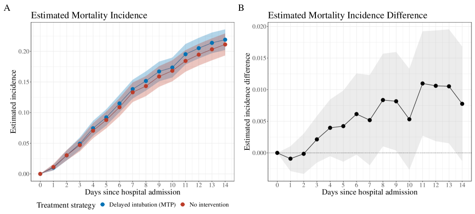
Figure 1: Panel A: Estimated incidence of mortality between a Delayed Intubation MTP (blue) and No intervention (red). Panel B: Estimated incidence difference in mortality if the Delayed Intubation MTP were implemented during Spring 2020. In both panels, 95% simultaneous confidence bands ³⁸ cover the sets of point estimates.

8 Discussion

The LMTP framework provides a unified and comprehensive approach for defining, identifying, and estimating relevant causal parameters, including those that involve challenges such as loss-to-follow-up, survival analysis, missing exposures, competing risks, and interventions that include multiple exposures and/or continuous exposures. These causal parameters may be formulated to reduce positivity violations. In addition, the existing packages that implement doubly and sequentially robust estimators enable researchers to take advantage of statistical learning algorithms to estimate the intervention and outcome mechanisms, thereby increasing the likelihood of estimator consistency.

While the LMTP framework expands the applied researcher’s toolbox, there are considerations and limitations to its implementation in real-world applications. First, using it in a longitudinal setting requires discretizing time over intervals. Depending on the data collection process, this may cause issues in temporality or loss of data granularity. This discretization may also cause issues in small sample sizes if there are very few outcomes within a certain time point and the applied researcher hopes to estimate the outcome regressions using any statistical learning algorithm which segments the data for training/testing. Second, although the formulation of MTPs may alleviate positivity violations, some violations may still occur. Possible solutions, such as truncating the density ratios at a certain threshold, are arbitrary and the potential for bias is unclear. Third, some particular estimator applications may be computationally intensive. Despite these limitations, we hope the overview of LMTPs, illustrative example, and corresponding Github repository are a useful toolset for researchers hoping to implement LMTPs into their applied work.

9 Tables

Table 1: An overview of common intervention types in the causal inference literature and whether they are estimable using the lmtp R package.

Intervention and definition	Estimable with lmtp?
Static: all units receive the same treatment assignment	Yesa
Dynamic: A unit’s treatment assignment is determined according to their prior exposure and/or covariate history	Yesa
Stochastic: A unit’s treatment assignment is determined via a randomization component, and possibly their prior exposure or covariate history	See assumptionsb
Modified: A unit’s treatment assignment is determined according to their natural exposure value, and possibly their prior exposure or covariate history, and possibly with a randomization component	See assumptionsb

• The software should only be used with discrete exposures. The software will output a result with a continuous exposure, but this estimator will not have good statistical properties.

• Assumptions require the intervention function $\mathsf{d}$ does not depend on the distribution $\mathsf{P}$, and, one of: (1) the exposure is discrete or (2) the exposure is continuous but $\mathsf{d}$ satisfies piecewise smooth invertibility. This includes many, but not all, modified and stochastic interventions; see Technical Requirements in Appendix for more details.

Table 2: Comparison of statistical properties for five possible estimators for LMTPs: g-computation (G-COMP), inverse probability weighting (IPW), targeted maximum likelihood estimation (TMLE), sequentially doubly robust estimation (SDR), and iterative TMLE (iTMLE).

Statistical Property	G-COMP	IPW	TMLE	SDR	iTMLEa
Uses outcome regression	1F5F8		1F5F8	1F5F8	1F5F8
Uses treatment regression		1F5F8	1F5F8	1F5F8	1F5F8
Doubly robustb			1F5F8	1F5F8	1F5F8
Sequentially doubly robustc				1F5F8	1F5F8
Valid inferenced using parametric regressions (i.e. generalized linear models)	1F5F8	1F5F8	1F5F8	1F5F8	1F5F8
Valid inferenced using data-adaptive regressions (i.e. machine learning)			1F5F8	1F5F8	1F5F8
Guaranteed to stay within observed outcome range	1F5F8		1F5F8		1F5F8

• The iTMLE estimator is not currently available within the R package lmtp.

• The estimator is consistent as long as all outcome regressions for times $t>s$ are consistently estimated, and all treatment mechanisms for times $t\leq s$ are consistent, for some time $s$.

• The estimator is consistent if, for every time point, either the outcome regression or the treatment mechanism is consistently estimated.

• Includes standard errors, confidence intervals, and p-values.

Table 3: Examples of static, dynamic, stochastic, and modified interventions for (1) binary and (2) continuous point-in-time exposures defined via the generalized LMTP framework. These can be expanded to any categorical exposure. We denote a random variable drawn from Bernoulli distribution with probability $0.5$ with $\epsilon$ unless otherwise noted.

Exposure	Intervention	“What if…”	Shift Notation
Point-in-time Binary, e.g. vaping $(a=1)$	Static	no one vapes	$\mathsf{d}(a,h,\epsilon)=0$
	Dynamic	only those working non-standard work hours $(l^{*}=1)$ vape	$\mathsf{d}(a,h,\epsilon)=\begin{cases}1&\text{ if }l^{*}=1\\ 0&\text{ otherwise}\end{cases}$
	Stochastic	only a random half of those working non-standard work hours $(l^{*}=1)$ vape	$\mathsf{d}(a,h,\epsilon)=\begin{cases}\epsilon&\text{ if }l^{*}=1\\ 0&\text{ otherwise}\end{cases}$
	Modified	a random half of current vapers stop vaping	$\mathsf{d}(a,h,\epsilon)=\begin{cases}\epsilon&\text{ if }a=1\\ a&\text{ otherwise }\end{cases}$
Point-in-time Continuous, e.g. exposure to pollution as measured by the Air Quality Index (AQI) scale	Static	all counties are exposed to an AQI of 10	$\mathsf{d}(a,h,\epsilon)=10$
	Dynamic	all urban ($l^{*}=1$) counties are exposed to an AQI of 40 and all rural ($l^{*}=0$) counties are exposed to an AQI of 20	$\mathsf{d}(a,h,\epsilon)=\begin{cases}40&\text{ if }l^{*}=1\\ 20&\text{ otherwise}\end{cases}$
	Stochastic	all urban ($l^{*}=1$) counties are exposed to an AQI of $\epsilon_{1}\sim N(40,5)$ and all rural ($l^{*}=0$) counties are exposed to an AQI of $\epsilon_{0}\sim N(20,5)$	$\mathsf{d}(a,h,\epsilon)=\begin{cases}\epsilon_{1}&\text{ if }l^{*}=1\\ \epsilon_{0}&\text{ otherwise}\end{cases}$
	Modified	all counties with an AQI higher than 20 are exposed to an AQI 10% lower than what they were naturally exposed to	$\mathsf{d}(a,h,\epsilon)=\begin{cases}a\times 0.9&\text{ if }a>20\\ a&\text{ otherwise}\end{cases}$

Table 4: Examples of static, dynamic, stochastic, and modified interventions for a binary time-varying exposure defined via the generalized LMTP framework. We index study time at $t=0$ and denote a random variable drawn from Bernoulli distribution with probability $0.5$ with $\epsilon_{t}$.

Exposure	Intervention	“What if…”	Shift Notation
Time-varying Binary, e.g. corticosteroids receipt $(a_{t}=1)$	Static	all patients receive corticosteroids for the first 6 days of hospitalization	$\mathsf{d}_{t}(a_{t},h_{t},\epsilon_{t})=\begin{cases}1&\text{ if }t\leq 5\\ 0&\text{ otherwise}\end{cases}$
	Dynamic	patients receive corticosteroids for 6 days once they become hypoxic $(l^{*}_{t}=1)$	$\mathsf{d}_{t}(a_{t},h_{t},\epsilon_{t})=\begin{cases}1&\text{ if }l^{*}_{s}=1\text{ for }s\in\{t-5,\ldots,t\}\\ 0&\text{ otherwise}\end{cases}$
	Stochastic	a random half of hypoxic $(l^{*}_{t}=1)$ patients are given corticosteroids for 6 days	$\mathsf{d}_{t}(a_{t},h_{t},\epsilon_{t})=\begin{cases}\epsilon_{t}&\text{ if }l^{*}_{s}=1\text{ for }s\in\{t-5,\ldots,t\}\\ 0&\text{ otherwise}\end{cases}$
	Modified	patients’ receipt of corticosteroids is delayed by 1 day	$\mathsf{d}_{t}(a_{t},h_{t},\epsilon_{t})=\begin{cases}0&\text{ if }a_{t}=1\text{ and }a_{t-1}=0\\ a_{t}&\text{ otherwise}\end{cases}$

10 Appendix

10.1 Additional Intervention Examples

10.1.1 Stochastic Interventions

Example 8 (Incremental propensity score interventions based on the odds ratio).

A recently developed type of stochastic interventions is Kennedy ³⁹’s incremental propensity score interventions (IPSI), which shifts a unit’s probability of receiving treatment conditional on their according to some constant $\delta$. First, a shifted propensity score is defined:

$$\pi^{\mathsf{d}}_{t}(h_{t})=\frac{\delta\pi_{t}(h_{t})}{\delta\pi_{t}(h_{t})+1-\pi_{t}(h_{t})}$$

Then, a random variable $\epsilon_{t}$ is drawn from a uniform distribution in $(0,1)$ and the intervention is defined as:

$$\mathsf{d}_{t}(h_{t},\epsilon_{t},\pi_{t})=I(\epsilon_{t}<\pi^{\mathsf{d}}_{t}(h_{t})),$$

This IPSI is said to be based on an odds ratio because the odds ratio of $\pi^{\mathsf{d}}_{t}(h_{t})$ to $\pi_{t}(h_{t})$ is equal to $\delta$. Naimi et al. ⁴⁰ used an IPSI to study the causal relationship between vegetable density consumption and the risk of preeclampsia among pregnant women. They studied whether preeclampsia would increase if women’s propensity of eating a minimum amount of vegetables increased by an odds ratio of $\delta$, for example, $\delta=1.5$ would mean a woman with a propensity of 0.35 increases to 0.45.

10.1.2 Modified Treatment Policies

Example 9 (Incremental propensity score based on the risk ratio).

Another type of IPSI proposed by Wen et al. ⁴¹ begins with a slightly different set-up than Kennedy ³⁹. Instead of relying on the treatment mechanism, there is a random draw $\epsilon_{t}$ from a Uniform $(0,1)$ distribution. If the draw is less than some $\delta$, then the treatment assignment is the natural value of treatment. If not, it is some constant value, for example 0.

$$\text{$\mathsf{d}_{t}(a_{t},\epsilon_{t})$}=\begin{cases}\text{$a_{t}$ if $\epsilon_{t}<\delta$},\\ \text{$0$ otherwise}\end{cases}$$

This intervention is said to be based on the risk ratio because $\delta=\pi^{\mathsf{d}}_{t}(h_{t})/\pi_{t}(h_{t})$, where $\pi^{\mathsf{d}}_{t}(h_{t})$ is the post-intervention propensity score and $\pi_{t}(h_{t})$ is the propensity score in the observed data generating mechanism. Wen et al. ⁴¹ argue the risk ratio interpretation may be more intuitive for collaborators, and they demonstrate this IPSI in an application studying the effect of PrEP usage increases on sexually transmitted infection rates.

10.2 Estimation Algorithms

10.2.1 G-Computation Algorithm

The G-Computation algorithm steps and pseudo-code for a simple example with two time points is shown below.

1. Fit a generalized linear model (GLM) for $Y$ conditional on $A_{1}=a_{1}$ and $H_{1}=h_{1}$. Call this $\hat{Q_{1}}(a_{1},h_{1})$.

   Q1_hat $\leftarrow$ glm$(\text{outcome}=Y,\text{predictors}=\{H_{1},A_{1}\})$

2. Modify the data set used in step (1) so that the values in the column for $A_{1}$ are changed to $A^{\mathsf{d}}_{1}$. Obtain the predictions for the model $\hat{Q_{1}}$ using this modified data set. These are pseudo-outcomes $\tilde{Y}_{1}$.

   pseudo_Y1 $\leftarrow$ predict$(\text{fit}=\texttt{Q1\_hat},\text{new data}=\{H_{1},A_{1}=A_{1}^{\mathsf{d}}\})$

3. Fit a generalized linear model (GLM) for $\tilde{Y}_{1}$ conditional on $A_{0}=a_{0}$ and $H_{0}=h_{0}$. Call this $\hat{Q_{0}}(a_{0},h_{0})$.

   Q0_hat $\leftarrow$ glm$(\text{outcome}=\texttt{pseudo\_Y1},\text{predictors}=\{H_{0},A_{0}\})$

4. Modify the data set used in step (3) so that the values in the column for $A_{0}$ are changed to $A^{\mathsf{d}}_{0}$. Obtain the predictions for the model $\hat{Q_{0}}$ using this modified data set. These are pseudo-outcomes $\tilde{Y}_{0}$.

   pseudo_Y0 $\leftarrow$ predict$(\text{fit}=\texttt{Q1\_hat},\text{new data}=\{H_{0},A_{0}=A_{0}^{\mathsf{d}}\})$

5. Average $\tilde{Y}_{0}$, i.e. compute $\hat{\mathsf{E}}[\tilde{Y}_{0}]$.

   estimate $\leftarrow$ mean(pseudo_Y0)

10.2.2 Inverse Probability Weighting Algorithm

The IPW estimator relies on a density ratio $\mathsf{r}_{t}=\mathsf{g}_{t}^{\mathsf{d}}(a_{t}\mid h_{t})/\mathsf{g}_{t}(a_{t}\mid h_{t})$, where $\mathsf{g}_{t}^{\mathsf{d}}(a_{t}\mid h_{t})$ is the density of the intervened exposure, and $\mathsf{g}_{t}(a_{t}\mid h_{t})$ is the density of the naturally observed exposure. Practically, $\mathsf{r}_{t}$ can be computed using a clever classification trick proposed in Qin ⁴², Cheng and Chu ⁴³ and utilized in Díaz et al. ¹⁰. The IPW algorithm with pseudo-code for a simple example with two time points is as follows.

1. Duplicate each row of the data set so that there are $2n$ rows. The first row of a duplicated pair should contain observed values $A_{1}$, and the second row should be modified so that $A_{1}=A_{1}^{\mathsf{d}}$. A new column $\Lambda_{1}$ should be created that is $0$ if $A_{1}=A_{1}$ and $1$ if $A_{1}=A_{1}^{\mathsf{d}}$.

   data $\leftarrow$ matrix$(\{H_{1},A_{1},\Lambda_{1}=0\}\})$

   data_copy $\leftarrow$ matrix$(\{H_{1},A_{1}=A_{1}^{\mathsf{d}},\Lambda_{1}=1\})$

   dr_data $\leftarrow$ bind_rows(data, data_copy)

2. Fit a logistic regression for $\Lambda_{1}$ conditional on $A_{1}=a_{1}$ and $H_{1}=h_{1}$. The odds ratio at a given $a_{1}$ and $h_{1}$ is the estimate of the density ratio at time 1, $\hat{\mathsf{r}_{1}}$.

   r1_fit $\leftarrow$ glm$(\text{outcome}=\Lambda_{1},\text{predictors}=\{H_{1},A_{1}\},\text{data}=\texttt{dr\_data})$

   r1_hat $\leftarrow$ predict$(\text{fit}=\texttt{r1\_fit},\text{prediction = odds ratio},\text{new data = }\texttt{data})$

3. Create a new column in the duplicated data set which contains values of $A_{0}$ in the first row of a duplicated pair. The second row in a pair should be modified so that $A_{0}=A_{0}^{\mathsf{d}}$. A new column $\Lambda_{0}$ should be created that is $0$ if $A_{0}=A_{0}$ and $1$ if $A_{0}=A_{0}^{\mathsf{d}}$.

   

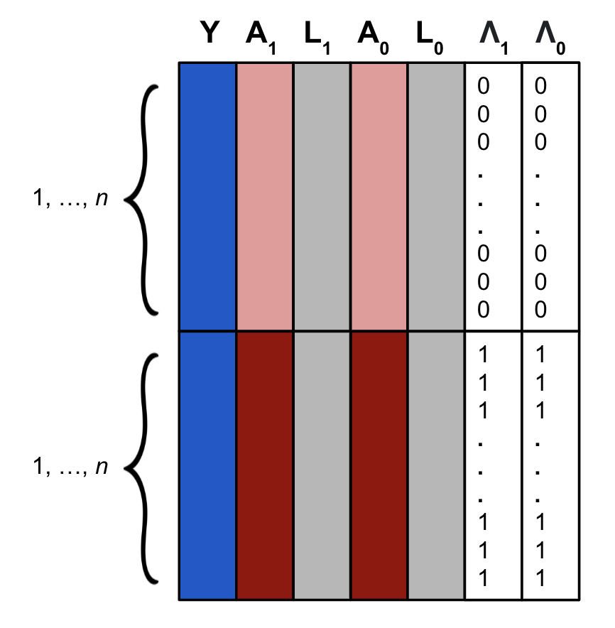
   Figure 2: Illustration of the data used for density ratio estimation with the classification trick.

4. Fit a logistic regression for $\Lambda_{0}$ conditional on $A_{0}=a_{0}$ and $H_{0}=h_{0}$. The odds ratio at a given $a_{0}$ and $h_{0}$ is the estimate of the density ratio at time 0, $\hat{\mathsf{r}_{0}}$.

   r0_fit $\leftarrow$ glm$(\text{outcome}=\Lambda_{0},\text{predictors}=\{H_{0},A_{0}\},\text{data}=\texttt{dr\_data})$

   r0_hat $\leftarrow$ predict$(\text{fit}=\texttt{r0\_fit},\text{prediction = odds ratio},\text{new data = }\texttt{data})$

5. Multiply $\hat{\mathsf{r}_{1}}$ and $\hat{\mathsf{r}_{0}}$ together. This is the cumulative density ratio. Multiply the cumulative density ratio by $Y$. Compute the average. This is $\hat{\mathsf{E}}[\tilde{Y}_{0}]$.

   estimate $\leftarrow$ mean(r1_hat * r0_hat * $Y)$

10.2.3 Technical requirements for theoretical guarantees of estimators

The $\sqrt{n}$-consistency and asymptotic normality of the estimators proposed in Díaz et al. ¹⁰, and therefore the correctness of the confidence intervals output by the R software lmtp ²⁰, ¹⁹, relies on two important technical requirements. First, the function $\mathsf{d}$ must not depend on the distribution of the data. Second, the exposure must be discrete or, if it is continuous, $\mathsf{d}(\cdot,h_{t},\epsilon_{t})$ (as a function of $a_{t}$) must be piecewise smooth invertible ¹, ¹⁰. If any of these reequirements is violated, important theoretical properties of the estimators such as $\sqrt{n}$-consistent will fail. This means that important uncertainty quantification measures such as confidence intervals, p-values, and standard errors outputted by the package will be incorrect.

If the first requirement is violated, it may be possible to develop $\sqrt{n}$-consistent estimators. For example, Kennedy ³⁹ developed non-parametric $\sqrt{n}$-consistent estimators for the IPSI shown in Example 8, in which $\mathsf{d}$ depends on the treatment mechanism. However, the IPSI proposed by Wen et al. ⁴¹ in Example 9, which does not depend on the data distribution, can be estimated with the proposed estimators. Here it is important to note that the the estimators for the odds ratio IPSI of Kennedy ³⁹ are not doubly robust (and such estimators possibly cannot be constructed, since $\mathsf{d}$ depends on the propensity score), whereas the estimators of the risk-ratio IPSI will be doubly robust.

If the second requirement is violated, it is not possible to construct $\sqrt{n}$-consistent estimators. Intuitively, this is due to a lack of “smoothness” in the parameter, and interested readers should refer to literature on pathwise differentiability an accessible review may be found in ⁴⁴. In Example 3, the static and dynamic interventions for corticosteroids administration are possible to estimate using the proposed estimators because the exposure is discrete. However, if the exposure were continuous (e.g. a dosage), this would not be possible. The modified threshold function (Example 6) also does not meet the second requirement because $\mathsf{d}$ is not piecewise smooth invertible. However, the modified shift functions (Example 7) meet both requirements and are estimable using the proposed estimators.

10.3 Practical guidance and considerations

In practice we recommend using TMLE if the user is not concerned about model misspecification, because the estimates are guaranteed to remain within the observed outcome bounds. However, if model misspecification is a concern, SDR is significantly more robust, although there is a potential for estimates which fall outside the outcome bounds. An effective approach against model misspecification is to use the superlearner algorithm for estimating the exposure and outcome mechanisms. Superlearning combines the predictions of multiple pre-specified statistical learning models via weighting to produce final estimates which are proven to perform as well as possible in large sample sizes ³⁷.

To assess positivity violations, we recommend the researcher to visually inspect or examine summary statistics of the density ratios. Extremely high values of density ratios (the quantification of “high” being context-dependent) are akin to propensity score values at or near zero, generally indicate positivity violations, and may create unstable estimates. If violations are detected, the researcher may be interested in modifying the portion of the population receiving the intervention, or in cases of continuous exposures, making the intervened exposure level closer to the observed exposure level. Interventions should be designed to avoid both theoretical and practical positivity violations present in the data, the latter of which can potentially be caught in the exploratory data analysis stage. One option if the researcher cannot find a solution by study design to elimitate positivity violations is to truncate the density ratios as a certain threshold, e.g. the 98th quantile. This is akin to truncating a propensity score, and may have potential for biases ⁴⁵.

Analysts using the LMTP framework for time-varying or survival outcomes will also note that discrete outcome intervals are required. The researcher must find a balance in choosing intervals that are both scientifically relevant (e.g. week-long intervals for a critically ill patient population would be too long) and in which there are still a number of outcomes which occur within the chosen interval. If the outcome is rare and the sample size is small, or if the sample size is very large and computationally intensive, the researcher may need to adjust the number of cross-fitting and/or superlearning cross-validation folds.

10.4 Additional Application Details

10.4.1 Methods

Baseline confounders include age, sex, race, ethnicity, body mass index (BMI), comorbidities (cerebral vascular event, hypertension, diabetes mellitus, cirrhosis, chronic obstructive pulmonary disease, active cancer, asthma, interstitial lung disease, chronic kidney disease, immunosuppression, HIV-infection, and home oxygen use), and hospital admission location. Time-dependent confounders include vital signs (heart rate, pulse oximetry percentage, respiratory rate, temperature, systolic/diastolic blood pressure), laboratory results (blood urea nitrogen (BUN)- creatinine ratio, creatinine, neutrophils, lymphocytes, platelets, bilirubin, blood glucose, D-dimers, C-reactive protein, activated partial thromboplastin time, prothrombin time, arterial partial pressures of oxygen and carbon dioxide), and concurrent pharmaceutical treatments. Concurrent treatments included vasopressors, diuretics, Angiotensin-converting enzyme (ACE) and Angiotensin receptor blockers (ARBs), hydroxychloroquine, and tocilizumab.

In the case of multiple time-varying confounders measured in one day, the clinically worst value was used. Although data was relatively complete due to manual abstraction efforts, there were instances of patients missing laboratory results at one or multiple time points. A combination of last observation carried forward and an indicator for missing values was used to handle this informative missingness within the treatment and regression models ⁴⁶.

The Superlearner ensemble algorithm utilized 5-fold cross-validation and candidate libraries included generalized linear models, multivariate adaptive regression splines ⁴⁷, random forests ⁴⁸, and extreme gradient boosted trees ⁴⁹ An assumption was made that the time-varying covariates from the previous two days (i.e. lag of 2 days) was sufficient to capture the mechanisms to reflect the collection of laboratory results at minimum 48-hour intervals. A 5-fold cross-fitting component was implemented for the final estimator to prevent variation in a certain sample split from biasing the final estimate ⁵⁰. All analyses were conducted in R Version 4.1.2 with the packages tidyverse ⁵¹ for data cleaning and plotting, and lmtp ¹⁹ and SuperLearner ⁵² for estimation.

10.4.2 Discussion

There are limitations specific to our illustrative example. While the estimated effect of a less aggressive intubation strategy can help to understand an underlying biological or mechanistic process, it may not provide clinical guidance if the treatment strategy changes over time. The estimates themselves depend on the natural value of treatment, and this is dependent on the state of clinical practice during the study time frame (Spring 2020). In addition, we cannot rule out unmeasured confounding in the exposure, outcome, and loss to follow-up mechanisms. We also cannot be sure whether the informative right censoring is correctly specified, since patients were lost to follow-up for different reasons (e.g. discharge to home vs. assisted living).

References

- Haneuse and Rotnitzky 2013 Sebastian Haneuse and Andrea Rotnitzky. Estimation of the effect of interventions that modify the received treatment. Statistics in medicine, 32(30):5260–5277, 2013.
- Cain et al. 2010 Lauren E Cain, James M Robins, Emilie Lanoy, Roger Logan, Dominique Costagliola, and Miguel A Hernán. When to start treatment? a systematic approach to the comparison of dynamic regimes using observational data. The international journal of biostatistics, 6(2), 2010.
- Petersen et al. 2012 Maya L Petersen, Kristin E Porter, Susan Gruber, Yue Wang, and Mark J van der Laan. Diagnosing and responding to violations in the positivity assumption. Statistical methods in medical research, 21(1):31–54, 2012.
- Young et al. 2014 Jessica G. Young, Miguel A. Hernán, and James M. Robins. Identification, estimation and approximation of risk under interventions that depend on the natural value of treatment using observational data. Epidemiologic Methods, 3(1):1–19, 2014. doi: doi:10.1515/em-2012-0001. URL https://doi.org/10.1515/em-2012-0001.
- Robins et al. 2004 James M Robins, Miguel A Hernán, and Uwe Siebert. Effects of multiple interventions. Comparative quantification of health risks: global and regional burden of disease attributable to selected major risk factors, 1:2191–2230, 2004.
- Taubman et al. 2009 Sarah L Taubman, James M Robins, Murray A Mittleman, and Miguel A Hernán. Intervening on risk factors for coronary heart disease: an application of the parametric g-formula. International journal of epidemiology, 38(6):1599–1611, 2009.
- Shpitser and Pearl 2012 Ilya Shpitser and Judea Pearl. Effects of treatment on the treated: Identification and generalization. arXiv preprint arXiv:1205.2615, 2012.
- Díaz and van der Laan 2012 Iván Díaz and Mark van der Laan. Population intervention causal effects based on stochastic interventions. Biometrics, 68(2):541–549, 2012.
- Richardson and Robins 2013 Thomas S Richardson and James M Robins. Single world intervention graphs (swigs): A unification of the counterfactual and graphical approaches to causality. Center for the Statistics and the Social Sciences, University of Washington Series. Working Paper, 128(30):2013, 2013.
- Díaz et al. 2021 Iván Díaz, Nicholas Williams, Katherine L. Hoffman, and Edward J. Schenck. Nonparametric Causal Effects Based on Longitudinal Modified Treatment Policies. Journal of the American Statistical Association, pages 1–16, September 2021. ISSN 0162-1459, 1537-274X. doi: 10.1080/01621459.2021.1955691. URL https://www.tandfonline.com/doi/full/10.1080/01621459.2021.1955691.
- Pearl 1998 Judea Pearl. Graphs, causality, and structural equation models. Sociological Methods & Research, 27(2):226–284, 1998.
- Pearl et al. 2016 Judea Pearl, Madelyn Glymour, and Nicholas P Jewell. Causal inference in statistics: A primer. 2016. Google Ascholar there is no corresponding record for this reference, 2016.
- Hernán et al. 2006 Miguel A Hernán, Emilie Lanoy, Dominique Costagliola, and James M Robins. Comparison of dynamic treatment regimes via inverse probability weighting. Basic & clinical pharmacology & toxicology, 98(3):237–242, 2006.
- Hoffman et al. 2022 Katherine L Hoffman, Edward J Schenck, Michael J Satlin, William Whalen, Di Pan, Nicholas Williams, and Iván Díaz. Comparison of a target trial emulation framework vs cox regression to estimate the association of corticosteroids with covid-19 mortality. JAMA Network Open, 5(10):e2234425–e2234425, 2022.
- van der Laan and Rose 2018 Mark J van der Laan and Sherri Rose. Targeted learning in data science. Springer, 2018.
- Robins 1986 James M Robins. A new approach to causal inference in mortality studies with sustained exposure periods - application to control of the healthy worker survivor effect. Mathematical Modelling, 7:1393–1512, 1986.
- Bang and Robins 2005 Heejung Bang and James M Robins. Doubly robust estimation in missing data and causal inference models. Biometrics, 61(4):962–973, 2005.
- van der Laan et al. 2011 Mark J van der Laan, Sherri Rose, et al. Targeted learning: causal inference for observational and experimental data, volume 10. Springer, 2011.
- Williams and Díaz 2021 Nicholas T Williams and Iván Díaz. lmtp: Non-parametric Causal Effects of Feasible Interventions Based on Modified Treatment Policies, 2021. URL https://github.com/nt-williams/lmtp. R package version 1.3.1.
- Williams and Díaz 2023 Nicholas Williams and Iván Díaz. lmtp: An r package for estimating the causal effects of modified treatment policies. Observational Studies, 9(2):103–122, 2023.
- van der Laan and Gruber 2012 Mark J van der Laan and Susan Gruber. Targeted minimum loss based estimation of causal effects of multiple time point interventions. The international journal of biostatistics, 8(1), 2012.
- Luedtke et al. 2017 Alexander R Luedtke, Oleg Sofrygin, Mark J van der Laan, and Marco Carone. Sequential double robustness in right-censored longitudinal models. arXiv preprint arXiv:1705.02459, 2017.
- Rotnitzky et al. 2017 Andrea Rotnitzky, James Robins, and Lucia Babino. On the multiply robust estimation of the mean of the g-functional. arXiv preprint arXiv:1705.08582, 2017.
- Díaz et al. 2022 Iván Díaz, Katherine L Hoffman, and Nima S Hejazi. Causal survival analysis under competing risks using longitudinal modified treatment policies. arXiv preprint arXiv:2202.03513, 2022.
- Nugent and Balzer 2021 Joshua R Nugent and Laura B Balzer. Evaluating shifts in mobility and covid-19 case rates in us counties: A demonstration of modified treatment policies for causal inference with continuous exposures. arXiv preprint arXiv:2110.12529, 2021.
- Rudolph et al. 2022 Kara E Rudolph, Catherine Gimbrone, Ellicott C Matthay, Iván Díaz, Corey S Davis, Katherine Keyes, and Magdalena Cerdá. When effects cannot be estimated: redefining estimands to understand the effects of naloxone access laws. Epidemiology, 33(5):689–698, 2022.
- Milazzo et al. 2023 Floriana Milazzo, Katherine L. Hoffman, Nicholas Williams, Rourke O’Brien, and Kara E. Rudolph. The association between disability application success and denial rates and drug overdoses. ArXiv, 2023.
- Jafarzadeh et al. 2022 S Reza Jafarzadeh, Tuhina Neogi, Daniel K White, and David T Felson. The relationship of pain reduction with prevention of knee replacement under dynamic intervention strategies. Arthritis & Rheumatology, 74(10):1668–1675, 2022.
- Huling et al. 2022 Jared D Huling, Robin R Austin, Sheng-Chieh Lu, Mary M Doran, Vicki J Swarr, and Karen A Monsen. Public health nurse tailored home visiting and parenting behavior for families at risk for referral to child welfare services, colorado: 2018–2019. American Journal of Public Health, 112(S3):S306–S313, 2022.
- Mehta et al. 2021 Bella Mehta, Collin Brantner, Nicholas Williams, Jackie Szymonifka, Iris Navarro-Millan, Lisa A Mandl, Anne R Bass, Linda A Russell, Michael L Parks, Mark P Figgie, et al. Primary care provider density and elective total joint replacement outcomes. Arthroplasty today, 10:73–78, 2021.
- Tobin et al. 2020 Martin J Tobin, Franco Laghi, and Amal Jubran. Caution about early intubation and mechanical ventilation in covid-19. Annals of intensive care, 10(1):1–3, 2020.
- Perkins et al. 2020 Gavin D Perkins, Keith Couper, Bronwen Connolly, J Kenneth Baillie, Judy M Bradley, Paul Dark, Anthony De Soyza, Ellen Gorman, Alasdair Gray, Louisa Hamilton, et al. Recovery-respiratory support: respiratory strategies for patients with suspected or proven covid-19 respiratory failure; continuous positive airway pressure, high-flow nasal oxygen, and standard care: a structured summary of a study protocol for a randomised controlled trial. Trials, 21:1–3, 2020.
- Goyal et al. 2020 Parag Goyal, Justin J Choi, Laura C Pinheiro, Edward J Schenck, Ruijun Chen, Assem Jabri, Michael J Satlin, Thomas R Campion Jr, Musarrat Nahid, Joanna B Ringel, et al. Clinical characteristics of covid-19 in new york city. New England Journal of Medicine, 382(24):2372–2374, 2020.
- Schenck et al. 2021 Edward J Schenck, Katherine L Hoffman, Marika Cusick, Joseph Kabariti, Evan T Sholle, and Thomas R Campion Jr. Critical care database for advanced research (cedar): An automated method to support intensive care units with electronic health record data. Journal of Biomedical Informatics, 118:103789, 2021.
- Wolpert 1992 David H Wolpert. Stacked generalization. Neural Networks, 5(2):241–259, 1992.
- Breiman 1996 Leo Breiman. Stacked regressions. Machine Learning, 24(1):49–64, 1996.
- van der Laan et al. 2007 Mark J van der Laan, Eric C Polley, and Alan E Hubbard. Super learner. Statistical Applications in Genetics & Molecular Biology, 6(25):Article 25, 2007.
- Westling et al. 2020 Ted Westling, Mark J van der Laan, and Marco Carone. Correcting an estimator of a multivariate monotone function with isotonic regression. Electronic journal of statistics, 14(2):3032, 2020.
- Kennedy 2019 Edward H Kennedy. Nonparametric causal effects based on incremental propensity score interventions. Journal of the American Statistical Association, 114(526):645–656, 2019.
- Naimi et al. 2021 Ashley I Naimi, Jacqueline E Rudolph, Edward H Kennedy, Abigail Cartus, Sharon I Kirkpatrick, David M Haas, Hyagriv Simhan, and Lisa M Bodnar. Incremental propensity score effects for time-fixed exposures. Epidemiology (Cambridge, Mass.), 32(2):202, 2021.
- Wen et al. 2021 Lan Wen, Julia L Marcus, and Jessica G Young. Intervention treatment distributions that depend on the observed treatment process and model double robustness in causal survival analysis. Statistical Methods in Medical Research, page 09622802221146311, 2021.
- Qin 1998 Jing Qin. Inferences for case-control and semiparametric two-sample density ratio models. Biometrika, 85(3):619–630, 1998.
- Cheng and Chu 2004 Kuang Fu Cheng and Chih-Kang Chu. Semiparametric density estimation under a two-sample density ratio model. Bernoulli, 10(4):583–604, 2004.
- Kennedy 2022 Edward H Kennedy. Semiparametric doubly robust targeted double machine learning: a review. arXiv preprint arXiv:2203.06469, 2022.
- Léger et al. 2022 Maxime Léger, Arthur Chatton, Florent Le Borgne, Romain Pirracchio, Sigismond Lasocki, and Yohann Foucher. Causal inference in case of near-violation of positivity: comparison of methods. Biometrical Journal, 64(8):1389–1403, 2022.
- Burton and Altman 2004 A Burton and DG Altman. Missing covariate data within cancer prognostic studies: a review of current reporting and proposed guidelines. British journal of cancer, 91(1):4–8, 2004.
- Milborrow. 2021 Stephen Milborrow. earth: Multivariate Adaptive Regression Splines, 2021. URL https://CRAN.R-project.org/package=earth. R package version 5.3.1.
- Wright and Ziegler 2017 Marvin N. Wright and Andreas Ziegler. ranger: A fast implementation of random forests for high dimensional data in C++ and R. Journal of Statistical Software, 77(1):1–17, 2017. doi: 10.18637/jss.v077.i01.
- Chen et al. 2021 Tianqi Chen, Tong He, Michael Benesty, Vadim Khotilovich, Yuan Tang, Hyunsu Cho, Kailong Chen, Rory Mitchell, Ignacio Cano, Tianyi Zhou, Mu Li, Junyuan Xie, Min Lin, Yifeng Geng, and Yutian Li. xgboost: Extreme Gradient Boosting, 2021. URL https://CRAN.R-project.org/package=xgboost. R package version 1.5.0.2.
- Zivich and Breskin 2021 Paul N Zivich and Alexander Breskin. Machine learning for causal inference: on the use of cross-fit estimators. Epidemiology (Cambridge, Mass.), 32(3):393, 2021.
- Wickham et al. 2019 Hadley Wickham, Mara Averick, Jennifer Bryan, Winston Chang, Lucy D’Agostino McGowan, Romain François, Garrett Grolemund, Alex Hayes, Lionel Henry, Jim Hester, Max Kuhn, Thomas Lin Pedersen, Evan Miller, Stephan Milton Bache, Kirill Müller, Jeroen Ooms, David Robinson, Dana Paige Seidel, Vitalie Spinu, Kohske Takahashi, Davis Vaughan, Claus Wilke, Kara Woo, and Hiroaki Yutani. Welcome to the tidyverse. Journal of Open Source Software, 4(43):1686, 2019. doi: 10.21105/joss.01686.
- Polley et al. 2021 Eric Polley, Erin LeDell, Chris Kennedy, and Mark van der Laan. SuperLearner: Super Learner Prediction, 2021. URL https://CRAN.R-project.org/package=SuperLearner. R package version 2.0-28.