An Augmented Subspace Based Adaptive Proper Orthogonal Decomposition Method for Time Dependent Partial Differential Equations

Abstract

In this paper, we propose an augmented subspace based adaptive proper orthogonal decomposition (POD) method for solving the time dependent partial differential equations. By augmenting the POD subspace with some auxiliary modes, we obtain an augmented subspace. We use the difference between the approximation obtained in this augmented subspace and that obtained in the original POD subspace to construct an error indicator, by which we obtain a general framework for augmented subspace based adaptive POD method. We then provide two strategies to obtain some specific augmented subspaces, the random vector based augmented subspace and the coarse-grid approximations based augmented subspace. We apply our new method to two typical 3D advection-diffusion equations with the advection being the Kolmogorov flow and the ABC flow. Numerical results show that our method is more efficient than the existing adaptive POD methods, especially for the advection dominated models.

Mathematics Subject Classification. 65M60 65M55

Received: date / Accepted: date

Keywords

Proper orthogonal decomposition $\cdot$ Adaptive $\cdot$ Augmented subspace $\cdot$ Galerkin projection $\cdot$ Error indicator

1 Introduction

Time dependent partial differential equations arise in many important fields, e.g., the seawater intrusion [2], the heat transfer [10], semiconductor devices [39] and fluid equations [23; 3; 40; 60; 57; 36]. The study about the numerical methods for the time dependent partial differential equations is an important and attractive research topic. There are some classical numerical discretization methods for the spatial discretization of the time dependent partial differential equations, e.g., the finite element method [7], the finite difference method [52] and the plane wave method [28]. Usually, the semi-discretized systems resulted from applying these classical spatial discertization methods for a time dependent partial differential equations are huge dimensional. If we use these classical spatial discretization methods at each time interval, the computational cost will be very expensive, especially for complex systems.

Therefore, some efficient and accurate model order reduction methods have been proposed to reduce the dimension of discretized system and then the computational costs [4; 47; 11; 38; 6]. The basic idea for the model order reduction method is to project the continuous system onto a low-dimensional approximation subspace whose dimension is significantly less than that of the classical discretization space. Proper orthogonal decomposition (POD) is a commonly used model order reduction technique [22; 31; 46; 37; 19]. The typical steps for getting a POD reduced order model of a time dependent partial differential equation are as follows. First, choose some classical discretized method to discretize the continuous equation for some time interval, and solve the resulted high-dimensional discretized systems to get a set of snapshots. Then, construct the POD modes by minimizing the error between these modes and the snapshots, which is equivalent to solving an $N_{s}$ dimensional eigenvalue problem [51; 23; 49]. Here $N_{s}$ is the number of snapshots. At last, project the original system on the subspace spanned by the POD modes, which is also called POD subspace, and solve the resulted discretized systems in the following time intervals. In the actual calculation, singular value decomposition (SVD) is usually used to obtain the POD modes from the snapshots [35; 46; 9]. By choosing the snapshots properly, the number of the POD modes will usually be of magnitude smaller than the degrees of freedom resulted by the classical spacial discretization methods.

There are many applications of the POD methods in scientific and engineering field. For instance, in [15], a group proper orthogonal decomposition (GPOD) method was introduced to simulate the nonlinear Burgers equation. In [33], the POD method was used to solve the time-domain Maxwell’s equations. In [32], a reduced-order finite element formulation based on POD method was established for the Allen-Cahn equation. Other applications include studies of turbulence [17; 53], process identification [25; 26] and control in chemical engineering [42; 59], etc. We refer to [55; 56] for more introduction to the POD method.

There are also some existing works on the error analysis for the POD method. For example, Kunisch and Volkwein estimated the error of the POD approximation for linear and nonlinear evolution equations in [29; 30]. In [20], Xin et al. analyzed the convergence of the POD approximation for viscous G-equation by decomposing the data into a mean-free part and a mean part. More works about the numerical analysis for the POD method can be referred to [24; 34; 27] and references therein.

The classical POD method for time dependent partial differential equations only uses the snapshots obtained in the early time interval to construct the POD modes. Once the POD modes are obtained, they will be fixed and not updated during the time evolution any more. However, the solution of the system may change a lot over time. Therefore, if the POD modes are not updated as the time evolution, the approximation error obtained by the POD methods may become larger and larger.

In order to improve the accuracy of the POD methods in the whole time interval, some adaptive POD methods which update the POD modes as time evolution have been introduced in recent years [12; 13; 48; 54; 43]. In [12; 48; 54], the authors constructed some residual type error estimators, based on which some residual based adaptive POD methods are proposed for simulation of time dependent problems. In [13], the authors proposed a two-grid based adaptive POD method. For this method, they first constructed two finite element spaces, a coarse finite element space and a fine finite element space, and then used the error obtained in the coarse finite element space to construct the error indicator, by which people then knew if it is needed to update the POD subspace in the fine mesh or not. We refer to [13] for more details about the two-grid based adaptive POD method.

In this paper, we propose a new approach for developing some adaptive POD methods for the time dependent partial differential equations. The main idea of our approach is to add some auxiliary modes to the POD subspace to build an augmented subspace. We then use the difference between the approximation obtained in the augmented subspace and that obtained in original POD subspace to develop an error indicator. Using this idea, we obtain a general framework for augmented subspace based adaptive POD method. We then provide two specific methods to obtain the auxiliary mode, one is simply using a randomly generated vector as the auxiliary mode, the other is using a coarse-grid approximation as the auxiliary mode. Using the coarse-grid approximation to build the augmented subspace is inspired by [13]. In [13], the authors used the error obtained in a coarse finite element space to act as the error indicator, while in this paper, we use the approximation in the coarse finite element space to augment the POD subspace, and then develop an error indicator.

The rest of this paper is organized as follows. In Section 2, we give some preliminaries, including the general framework of the adaptive POD method, the complexity of the POD type methods and the simple descriptions of two typical adaptive POD methods. In Section 3, we propose a general framework for the augmented subspace based adaptive POD method, and provide two specific methods to construct the augmented subspace, the random vector based augmented subspace and the coarse grid approximations based augmented subspace. In Section 4, we apply the coarse-grid approximations based adaptive POD method to the simulation of some typical time dependent partial differential equations, i.e., the advection-diffusion equation with three dimensional velocity field, including both the Kolmogorov flow and the ABC flow. The numerical results show the accuracy and efficiency of our new method. In Section 5, we give some concluding remarks. Finally, we provide some additional numerical results for the advection dominated models with different coarse meshes and different error indicator threshold in “Appendix A”.

2 Preliminaries

We first recall some definition and notation. We shall use the standard notation for Sobolev spaces and their associated norms and seminorms; see, e.g., [1]. Let $V$ be a Banach space with norm $\|*\|_{V}$ and $L^{p}(0,T;V)$ be a Banach space equipped with the norm

$$\|u\|_{L^{p}(0,T;V)}=\left(\int^{T}_{0}\|u(t)\|_{V}^{p}\textup{d}t\right)^{\frac{1}{p}},1\leq p<\infty.$$

We call $u\in C(0,T;V)$ if

$$\|u\|_{C(0,T;V)}=\mathop{\max}\limits_{t\in[0,T]}\|u(t)\|_{V}<\infty.$$

In this paper, vectors and matrices will be denoted by bold letters.

We consider the following general time dependent partial differential equations:

$$\left\{\begin{aligned} &u_{t}-\epsilon\Delta u+{\bf B}(x,y,z,t)\cdot\nabla u+c(x,y,z,t)u=f(x,y,z,t),\quad\text{in}~{}\Omega\times(0,T]\\ &u(x,y,z,0)=h(x,y,z),\\ &u(x+\kappa,y,z,t)=u(x,y+\kappa,z,t)=u(x,y,z+\kappa,t)=u(x,y,z,t),\end{aligned}\right.$$ (2.1)

where $\Omega=[0,\kappa]^{3}$, $f\in L^{2}(0,T;L^{2}(\Omega))$, $c\in L^{\infty}(\Omega)$, ${\bf B}\in C(0,T;W^{1,\infty}(\Omega)^{3})$ and $\epsilon$ is a constant. We take an inner product with $v$ in (2.1) and define a bilinear form to simplify the variational form

$$a(t;u,v)=\epsilon(\nabla u,\nabla v)-\epsilon\int_{\partial\Omega}\frac{\partial u}{\partial n}vd\sigma+({\bf B}\cdot\nabla u,v)+(cu,v),\forall u,v\in H^{1}(\Omega),$$

where $(\cdot,\cdot)$ stands for the inner product in $L^{2}(\Omega)$. We can obtain the variational form of the Eq. (2.1) as follows: find $u\in L^{2}(0,T;V)$, $u_{t}\in L^{2}(0,T;V^{*})$ such that

$$(\frac{\partial u}{\partial t},v)+a(t;u,v)=(f(x,y,z,t),v),\forall v\in V,$$ (2.2)

where

$$V=\{v\in H^{1}(\Omega):v|_{x=0}=v|_{x=\kappa},v|_{y=0}=v|_{y=\kappa},v|_{z=0}=v|_{z=\kappa}\},$$

and $V^{*}$ is the dual space of V.

2.1 Standard discretization

We first consider the standard temporal discretization of (2.2). There are many existing temporal discretization methods, such as Euler method and implicit Euler method [21], which can be used to discretize (2.2). Here, we choose the implicit Euler method. We first divide the time interval into $N\in\mathbb{N}$ subintervals with equal length $\delta t=T/N$, and set $u^{k}(x,y,z)=u(x,y,z,t_{k})$, $f_{k}(x,y,z)=f(x,y,z,t_{k})$, where $t_{k}=k*\delta t$, for $k\in\{0,1,\cdots,N\}.$ Then we can get the semi-discretization scheme of (2.2) as follows:

$$\left(\frac{u^{k}(x,y,z)-u^{k-1}(x,y,z)}{\delta t},v\right)+a(t_{k};u^{k}(x,y,z),v)=(f_{k}(x,y,z),v),\quad v\in V.$$ (2.3)

We then consider the classical spatial discretization of (2.3). Here, we choose the finite element method to discretize (2.3). Let $\mathcal{T}_{h}$ be a shape regular family of nested conforming mesh over $\Omega$ with size $h$: there exists a constant $\gamma^{\ast}$ such that

$$\frac{h_{\tau}}{\rho_{\tau}}\leq\gamma^{\ast},\quad\forall~{}\tau\in\mathcal{T}_{h},$$ (2.4)

where $h_{\tau}$ is the diameter of $\tau$ for each $\tau\in\mathcal{T}_{h}$, $\rho_{\tau}$ is the diameter of the biggest ball contained in $\tau$, and $h=\max\{h_{\tau}:\tau\in\mathcal{T}_{h}\}$. Let $V_{h}$ be a subspace of continuous functions on $\Omega$ such that

$$V_{h}=\{v_{h}:v_{h}|_{\tau}\in\mathbb{P}_{\tau},\forall~{}\tau\in\mathcal{T}_{h}\mbox{ and }v_{h}\in C^{0}(\overline{\Omega})\},$$

where $\mathbb{P}_{\tau}$ is a set of polynomials on element $\tau$. Let $\{\phi_{h,1},\phi_{h,2},\cdots,\phi_{h,N_{g}}\}$ be a basis of $V_{h}$. Denote

$$\Phi_{h}:=(\phi_{h,1},\phi_{h,2},\cdots,\phi_{h,N_{g}}).$$

The standard finite element discretization of (2.3) can be formulated as follows: find $u^{k}_{h}(x,y,z)\in V_{h}$, such that

$$\left(\frac{u^{k}_{h}(x,y,z)-u^{k-1}_{h}(x,y,z)}{\delta t},v_{h}\right)+a(t_{k};u_{h}^{k}(x,y,z),v_{h})=(f_{k}(x,y,z),v_{h}),\quad v_{h}\in V_{h}.$$ (2.5)

Note that $u_{h}^{k}(x,y,z)$ can be expressed as

$$u^{k}_{h}(x,y,z)=\mathop{\sum}^{N_{g}}\limits_{i=1}u_{h,i}^{k}\phi_{h,i}(x,y,z).$$ (2.6)

Inserting (2.6) into (2.5), and setting $v_{h}=\phi_{h,j},j=1,2,\cdots,N_{g}$, respectively, we have

$$\left(\sum^{N_{g}}_{i=1}u_{h,i}^{k}\phi_{h,i}-\sum^{N_{g}}_{i=1}u_{h,i}^{k-1}\phi_{h,i},\phi_{h,j}\right)+\delta ta(t_{k};\sum^{N_{g}}_{i=1}u_{h,i}^{k}\phi_{h,i},\phi_{h,j})=\delta t(f_{k},\phi_{h,j}).$$ (2.7)

Define

$${\bf A}^{k}_{h,ij}=(\phi_{h,j},\phi_{h,i})+\delta ta(t_{k};\phi_{h,j},\phi_{h,i}),\quad {\bf u}^{k}_{h}=(u_{h,1}^{k},u_{h,2}^{k},\cdots,u_{h,N_{g}}^{k})^{T},$$

$${\bf b}^{k}_{h}=\delta t*((f_{k},\phi_{h,1}),\cdots,(f_{k},\phi_{h,N_{g}}))^{T},\quad {\bf C}_{h,ij}=(\phi_{h,j},\phi_{h,i}).$$

Then (2.7) can be rewritten as the following algebraic form

$${\bf A}^{k}_{h}{\bf u}^{k}_{h}={\bf b}^{k}_{h}+{\bf C}_{h}{\bf u}^{k-1}_{h}.$$ (2.8)

2.2 Adaptive POD method

In this subsection, we first recall the general procedure for getting a POD reduced order model of a time dependent partial differential equation. First, we choose some classical discretized method to discretize (2.3) in some time interval. Here we discretize (2.3) in the finite element space $V_{h}$ for $t\in[0,T_{0}]$, and solve the resulted high dimensional discretized systems at different times $t_{0}$, $t_{\delta M}$, $\cdots$, $t_{n_{s}\cdot\delta M}$ to get the snapshot matrix ${\bf U}_{h}$. Here, $\delta M$ is an integer parameter and $n_{s}=\lfloor\frac{T_{0}}{\delta t\cdot\delta M}\rfloor$, where $\lfloor*\rfloor$ means the round down. Then, we perform SVD on ${\bf U}_{h}$, and obtain ${\bf U}_{h}={\bf RSV^{T}}$. Note that the diagonal elements in S are arranged from largest to smallest, we set the number of POD modes by

$$m=\min\{k|\mathop{\sum}^{k}\limits_{i=1}{\bf S}_{i,i}>\gamma_{1}*{\rm Trace}({\bf S})\},$$ (2.9)

where $\gamma_{1}$ is a given parameter, and set ${\bf\widetilde{R}}={\bf R}[:,1:m]$. Then the POD modes are

$$\Psi_{h}=(\psi_{h,1},\psi_{h,2},\cdots,\psi_{h,m}):=\Phi_{h}{\bf\widetilde{R}}.$$

The process for constructing POD modes can be summarized as a routine POD_Mode(${\bf U}_{h},\gamma_{1},\Phi_{h},m,\Psi_{h}$) in Algorithm 1, see also [13].

Algorithm 1 POD_Mode(${\bf U}_{h},\gamma,\Phi_{h},m,\Psi_{h}$)

Input: ${\bf U}_{h},\gamma,\Phi_{h}=(\phi_{h,1},\phi_{h,2},\cdots,\phi_{h,n})$.
  Output: m and POD modes $\Psi_{h}=(\psi_{h,1},\psi_{h,2},\cdots,\psi_{h,m})$.

1:Perform SVD on ${\bf U}_{h}$ to obtain ${\bf U}_{h}={\bf RSV^{T}}$, where S = diag $\{\sigma_{1},\sigma_{2},\cdots,\sigma_{r}\}$ with $\sigma_{1}\geq\sigma_{2}\geq\cdots\geq\sigma_{r}>0.$

2:Set $m=min\{k|\mathop{\sum}^{k}\limits_{i=1}{\bf S}_{i,i}>\gamma*{\rm Trace}({\bf S})\}.$

3:$(\psi_{h,1},\psi_{h,2},\cdots,\psi_{h,m})=\Phi_{h}{\bf R}[:,1:m]$.

At last, we project (2.3) on the POD subspace $V_{h,\rm{POD}}=\text{span}\{\psi_{h,1},\cdots,\psi_{h,m}\}$ when $t>T_{0}$. The POD approximation $u^{k}_{h,\rm{POD}}$ is then expressed as

$$u^{k}_{h,\rm{POD}}(x,y,z)=\mathop{\sum}^{m}\limits_{i=1}\alpha_{h,i}^{k}\psi_{h,i}(x,y,z).$$ (2.10)

Inserting (2.10) into (2.3), and setting $v=\psi_{h,j},j=1,2,\cdots,m$, respectively, we obtain

$$\left(\sum^{m}_{i=1}\alpha_{h,i}^{k}\psi_{h,i}-\sum^{m}_{i=1}\alpha_{h,i}^{k-1}\psi_{h,i},\psi_{h,j}\right)+\delta ta(t_{k};\sum^{m}_{i=1}\alpha_{h,i}^{k}\psi_{h,i},\psi_{h,j})=\delta t(f_{k},\psi_{h,j}).$$ (2.11)

Define

$${\bf\bar{A}}^{k}_{h,ij}=(\psi_{h,j},\psi_{h,i})+\delta ta(t_{k};\psi_{h,j},\psi_{h,i}),\quad {\bf u}^{k}_{h,\rm{POD}}=(\alpha_{h,1}^{k},\alpha_{h,2}^{k},\cdots,\alpha_{h,m}^{k})^{T},$$

$${\bf\bar{b}}^{k}_{h}=\delta t*((f_{k},\psi_{h,1}),\cdots,(f_{k},\psi_{h,m}))^{T},\quad {\bf\bar{C}}_{h,ij}=(\psi_{h,j},\psi_{h,i}).$$

Then (2.11) can be rewritten as the following algebraic form

$${\bf\bar{A}}^{k}_{h}{\bf u}^{k}_{h,\rm{POD}}={\bf\bar{b}}^{k}_{h}+{\bf\bar{C}}_{h}{\bf u}^{k-1}_{h,\rm{POD}}.$$ (2.12)

From the expression of the POD modes, i.e., $\Psi_{h}=\Phi_{h}{\bf\widetilde{R}}$, the above equation can also be written as

$${\bf\widetilde{R}}^{T}{\bf A}^{k}_{h}{\bf\widetilde{R}}{\bf{u}}^{k}_{h,\rm{POD}}={\bf\widetilde{R}}^{T}{\bf b}^{k}_{h}+{\bf\widetilde{R}}^{T}{\bf C}_{h}{\bf\widetilde{R}}{\bf u}^{k-1}_{h,\rm{POD}}.$$

As we mentioned before, the classical POD method only uses the snapshots obtained in time interval $[0,T_{0}]$ to construct the POD modes. Once the POD modes are obtained, they will not be updated during the time evolution. However, the solution may change a lot over time. In order to improve the accuracy of the POD method in the whole time interval, more and more researchers have paid more attention to the study of adaptive POD method in recent years [12; 13; 48; 54; 43]. Here, we provide a briefly introduction to it.

Motivated by the procedure for adaptive finite element method [14], in [13], the authors summarized the procedure of adaptive POD method as a loop constructed by the following four steps:

1. Solve: Solve the Eq. (2.3) in the POD subspace $\text{span}\{\psi_{h,1},\cdots,\psi_{h,m}\}$.

2. Estimate: Construct an error indicator $\eta_{k}$ to estimate the error of the approximation obtained in current POD subspace.

3. Mark: Mark the time instance $t_{k}$ when the POD subspace is needed to be updated.

4. Update: Update the POD subspace at the marked time instance.

The step Solve is just the procedure for obtaining the approximations by the classical POD method we introduced above. The step Estimate is crucial for an adaptive POD method, which determines the efficiency and accuracy of the method. The step Mark picks out the time instance when the POD modes are needed to be updated. For the step Update, it is worthy of noting that, if the time instance $t=q\delta t$ is marked, we will go back to the previous time instance $t_{1}=(q-1)\delta t$ to restart the collection of the approximations in the finite element space and get the snapshots matrix ${\bf W}_{h,1}$. In order to obtain the new POD modes, we perform SVD on ${\bf W}_{h,1}$ to obtain ${\bf W}_{h,1}={\bf R}_{1}{\bf S}_{1}{\bf V}_{1}^{T}$. Then, we obtain the number of POD modes $m_{1}$ by (2.9) but with a different parameter $\gamma_{2}$. In order to keep the information in original POD modes, we perform SVD on ${\bf W}_{h,2}=[{\bf R}_{1}[:,1:m_{1}],{\bf\widetilde{R}}]$, and get ${\bf W}_{h,2}={\bf R}_{2}{\bf S}_{2}{\bf V}_{2}^{T}$. Then, we get the number of POD modes $m$ by (2.9) but with a parameter $\gamma_{3}$. Finally we set ${\bf\widetilde{R}}={\bf R}_{2}[:,1:m]$ and obtain the update POD modes by

$$\Psi_{h}=(\psi_{h,1},\psi_{h,2},\cdots,\psi_{h,m})=\Phi_{h}{\bf\widetilde{R}}.$$

For the convenience of the following discussion, we summarize the process for the step Update as routine Update_POD_Mode(${\bf W}_{h,1},\gamma_{2},\gamma_{3},\Phi_{h},m,\Psi_{h}$) in Algorithm 2, which is first introduced in [13].

Algorithm 2 Update_POD_Mode(${\bf W}_{h,1},\gamma_{2},\gamma_{3},\Phi_{h},m,\Psi_{h}$)

Input: ${\bf W}_{h,1},\gamma_{2},\gamma_{3},\Phi_{h}=(\phi_{h,1},\phi_{h,2},\cdots,\phi_{h,n})$, $m$ and $m$ old POD modes $\Psi_{h},\Psi_{h}=\Phi_{h}{\bf\widetilde{R}}$.
Output: new $m$ and new $m$ POD modes $\{\psi_{h,1},\psi_{h,2},\cdots,\psi_{h,m}$}.

1:Perform SVD on ${\bf W}_{h,1}$ to obtain ${\bf W}_{h,1}={\bf R}_{1}{\bf S}_{1}{\bf V}_{1}^{T}$, where ${\bf S_{1}}$ = diag$\{\sigma_{1,1},\sigma_{1,2},\cdots,\sigma_{1,r_{1}}\}$ with $\sigma_{1,1}\geq\sigma_{1,2}\geq\cdots\geq\sigma_{1,r_{1}}>0.$

2:Set $m_{1}={\rm min}\{k|\mathop{\sum}^{k}\limits_{i=1}{\bf S}_{1,ii}>\gamma_{2}*{\rm Trace}({\bf S}_{1})\}.$

3:Perform SVD on ${\bf W}_{h,2}=[{\bf R}_{1}[:,1:m_{1}],{\bf\widetilde{R}}]$, and obtain ${\bf W}_{h,2}={\bf R}_{2}{\bf S}_{2}{\bf V}_{2}^{T}$, where ${\bf S_{2}}$ = diag$\{\sigma_{2,1},\sigma_{2,2},\cdots,\sigma_{2,r_{2}}\}$ with $\sigma_{2,1}\geq\sigma_{2,2}\geq\cdots\geq\sigma_{2,r_{2}}>0.$

4:Set $m={\rm min}\{k|\mathop{\sum}^{k}\limits_{i=1}{\bf S}_{2,ii}>\gamma_{3}*{\rm Trace}({\bf S}_{2})\}$, and ${\bf\widetilde{R}}={\bf R}_{2}[:,1:m]$.

5:$(\psi_{h,1},\psi_{h,2},\cdots,\psi_{h,m})=\Phi_{h}{\bf\widetilde{R}}.$

We then obtain the framework of the adaptive POD method as Algorithm 3.

Algorithm 3 Framework of the adaptive POD method

1:Given $T_{0}$, $\delta M$, $\delta T$, $\delta t$,$\gamma_{1}$, $\gamma_{2}$, $\gamma_{3}$, $\eta_{0}$ and the mesh $\mathcal{T}_{h}$.

2:Discretize (2.3) in the standard finite element space $V_{h}$ on interval $[0,T_{0}]$ and obtain the snapshots matrix ${\bf U}_{h}$.

3:Construct POD modes $\Psi_{h}$ by POD_Mode(${\bf U}_{h},\gamma_{1},\Phi_{h},m,\Psi_{h}$).

4:$t=T_{0}$, $k=\frac{T_{0}}{\delta t}$.

5:while $t\leq T$ do

6:     $t=t+\delta t$, k = k + 1.

7:     Discretize (2.3) in the POD subspace $V_{h,\rm{POD}}=\text{span}\{\psi_{h,1},\psi_{h,2},\cdots,\psi_{h,m}\}$, and obtain the POD approximations ${\bf u}^{k}_{h,\rm{POD}}$.

8:     Compute the error indicator $\eta_{k}$ by some strategy.

9:     if $\eta_{k}>\eta_{0}$ then

10:         $t=t-\delta t$, k = k - 1.

11:         Discretize (2.3) in $V_{h}$ on interval $[t,t+\delta T]$ and get snapshots ${\bf W}_{h,1}$, then update POD modes $\Psi_{h}$ by Update_POD_Mode(${\bf W}_{h,1},\gamma_{2},\gamma_{3},\Phi_{h},m,\Psi_{h}$).

12:         $k=k+\frac{\delta T}{\delta t}$.      

13:     end if

14:end while

2.3 Complexity

In this subsection, we analyze the computational complexity of the standard finite element method, the standard POD method and the adaptive POD method introduced before. By comparing the computational complexity of these methods, the advantages of the POD type methods will be shown. We use $\mathcal{O}(n)$ to represent the complexity of a function that increases linearly with respect to $n$. For simplicity, we only consider the case that ${\bf B}$, $c$ and $f$ are separable in time and space, that is, ${\bf B}$ can be denoted as ${\bf B}(x,y,z,t)={\bf B_{1}}(x,y,z)+{\bf B_{2}}(x,y,z)B_{3}(t)$.

For the standard finite element method, the main computational costs at each time instance are those for building the discretized system and solving the discretized system. We first consider the cost for building the discretized system. We note that during the building of the linear system (2.8), only the terms $({\bf B}\cdot\nabla\phi_{h,j},\phi_{h,i})$, $(c\phi_{h,j},\phi_{h,i})$ and $(f,\phi_{h,i})$ are changed as the evolution of time. Let $N_{g}$ denote the degree of freedom for the finite element discretization. We only need to compute $({\bf B_{1}}\cdot\nabla\phi_{h,j},\phi_{h,i})$ and $({\bf B_{2}}\cdot\nabla\phi_{h,j},\phi_{h,i})$ once, and then multiply $({\bf B_{2}}\cdot\nabla\phi_{h,j},\phi_{h,i})$ by $B_{3}(t)$ at each time instance to obtain $({\bf B}\cdot\nabla\phi_{h,j},\phi_{h,i})$. For a fixed i, there are only finite j such that $(\nabla\phi_{h,j},\phi_{h,i})$ is not 0. This means the computational complexity of the multiplication by $B_{3}(t)$ is $\mathcal{O}(N_{g})$. Therefore, the computational complexity for building $({\bf B}\cdot\nabla\phi_{h,j},\phi_{h,i})$ is $\mathcal{O}(N_{g})$ at each time instance. Similarly, we have that the computational complexity for $(c\phi_{h,j},\phi_{h,i})$ and $(f,\phi_{h,i})$ is also $\mathcal{O}(N_{g})$. Therefore, the computational complexity for building the linear system (2.8) is $\mathcal{O}(N_{g})$. We then see the cost for solving the discretized linear system. For solution of (2.8), since ${\bf A}_{h}^{k}$ is sparse, there are many solvers [50; 44] which can deal with it at a cost of $\mathcal{O}(N_{g})$. Hence, the computational cost at each time instance is $\mathcal{O}(N_{g})$, and the total cost during $t\in[0,T]$ is $\mathcal{O}(N_{g})\times\frac{T}{\delta t}$.

We then turn to see the computational complexity for the standard POD method. When $t\in[0,T_{0}]$, we need to discrete the system (2.3) in the finite element space and then solve the discretized system (2.8). By the analysis for the standard finite element discretization, we know that the cost is $\mathcal{O}(N_{g})$ at each time instance. For the construction of the POD modes, we need to perform SVD on ${\bf U}_{h}\in\mathbb{R}^{N_{g}\times n_{s}}$, where $n_{s}=\lfloor\frac{T_{0}}{\delta t\cdot\delta M}\rfloor$ as we mentioned before. Since only the left singular vectors and the singular values need to be calculated, the computational complexity is $\mathcal{O}(n_{s}^{2}N_{g})$[18], where $n_{s}^{2}\ll N_{g}$. When $t>T_{0}$, we need to project (2.3) on the POD subspace and then solve the discretized system (2.12). The cost for building the linear system is $\mathcal{O}(N_{g})$ at each time instance. Since ${\bf B}$, $c$ and $f$ are separable in time and space, as we mentioned before, we only need to calculate $({\bf B_{1}}\cdot\nabla\psi_{h,j},\psi_{h,i})$ and $({\bf B_{2}}\cdot\nabla\psi_{h,j},\psi_{h,i})$ once, which costs $\mathcal{O}(N_{g})$, and then multiply it by $B_{3}(t)$ at each time instance to obtain $({\bf B}\cdot\nabla\psi_{h,j},\psi_{h,i})$, where $i,j=1,2,\cdots,m$. Since matrices composed by $({\bf B_{2}}\cdot\nabla\psi_{h,j},\psi_{h,i})$ and $(c\psi_{h,j},\psi_{h,i})$ are dense, the complexity of building the linear system (2.12) is $\mathcal{O}(m^{2})$ at each time instance. For solving the discretize system (2.12), since ${\bf\bar{A}}_{h}^{k}$ is a small dense matrix, we usually use some direct method to solve it, which costs $\mathcal{O}(m^{3})$. Therefore the total computational cost is $\mathcal{O}(N_{g})\times(\frac{T_{0}}{\delta t}+1)+\mathcal{O}(n_{s}^{2}N_{g})+\mathcal{O}(m^{3})\times\frac{T-T_{0}}{\delta t}$.

We now see the computational cost for the adaptive POD method. Except for the costs same as those for the standard POD method, some additional costs are needed for steps Estimate, Mark and Update. For the step Estimate, different methods have different ways to design the error indicator. We denote the computational cost for this part in each time instance as $t_{\rm est}$. The cost for the step Mark can be neglected. The main cost for the step Update is that for obtaining the standard finite element approximations on interval $[t,t+\delta T]$. From the analysis for the standard finite element method, we know that the cost for this part is $\mathcal{O}(N_{g})$ at each time instance. Let $n_{A}$ denote the number of updates for POD modes. Therefore, the total computational cost for SVD is $\mathcal{O}(n_{s}^{2}N_{g})\times 2n_{A}$. Since the number of POD modes will increase as the updating continues, we denote $m_{A}$ average number of POD modes in the adaptive POD method. By the analysis for the standard POD method, the cost for building the POD linear system is $\mathcal{O}(N_{g})\times n_{A}+\mathcal{O}(m_{A}^{2})\times\frac{T-T_{0}-n_{A}\delta T}{\delta t}$, and the cost for solving the discretized system at each time instance is $\mathcal{O}(m_{A}^{3})$. Therefore, the total computational cost is $\mathcal{O}(N_{g})\times(\frac{T_{0}+n_{A}\cdot\delta T}{\delta t}+n_{A}+1)+\mathcal{O}(n_{s}^{2}N_{g})\times(2n_{A}+1)+\mathcal{O}(m_{A}^{3})\times\frac{T-T_{0}-n_{A}\delta T}{\delta t}+t_{\rm est}\times\frac{T-T_{0}-n_{A}\delta T}{\delta t}$.

We summarize the total computational cost for each method in Table 1. Usually, we have $T_{0}\ll T$, $m^{3}\ll N_{g}$ and $m_{A}^{3}\ll N_{g}$. Therefore, we can see that the POD type methods usually cost less CPU time than the standard finite element method. Then we focus on the cost for the adaptive POD method. If an error indicator is cheaper, the term $t_{\rm est}$ will be less. If an error indicator is more sensitive, it will require fewer updates $n_{A}$ to achieve the same accuracy, then it may decrease the degree of freedom $m_{A}$ at the same time. Therefore, the construction of the error indicator plays an important role in reducing the cost for the adaptive POD method.

Table 1: Total complexity of different methods

Method	Complexity
standard finite element	$\mathcal{O}(N_{g})\times\frac{T}{\delta t}$
standard POD method	$\mathcal{O}(N_{g})\times(\frac{T_{0}}{\delta t}+1)+\mathcal{O}(n_{s}^{2}N_{g})+\mathcal{O}(m^{3})\times\frac{T-T_{0}}{\delta t}$
adaptive POD method	$\mathcal{O}(N_{g})\times(\frac{T_{0}+n_{A}\cdot\delta T}{\delta t}+n_{A}+1)+\mathcal{O}(n_{s}^{2}N_{g})\times(2n_{A}+1)$
	+ $\mathcal{O}(m_{A}^{3})\times\frac{T-T_{0}-n_{A}\delta T}{\delta t}+t_{\rm est}\times\frac{T-T_{0}-n_{A}\delta T}{\delta t}$

2.4 Typical existing adaptive POD methods

There are some existing works on adaptive POD methods [12; 48; 13]. The main difference between different adaptive POD methods lies in the construction of the error indicator. Here, we introduce two typical methods, one is the residual based adaptive POD method [12; 48], the other is the two-grid based adaptive POD method [13].

For the residual based adaptive POD method, the residual is used to construct the error indicator. In detail, the error indicator $\eta_{k}$ at time instance $t=k\delta t$ is defined as

$$\eta_{k}=\frac{\|{\bf A}_{h}^{k}{\bf\widetilde{R}}{\bf{u}}^{k}_{h,\rm{POD}}-{\bf b}_{h}^{k}-{\bf C}_{h}{\bf\widetilde{R}}{\bf{u}}^{k-1}_{h,\rm{POD}}\|_{2}}{\|{\bf b}_{h}^{k}+{\bf C}_{h}{\bf\widetilde{R}}{\bf{u}}^{k-1}_{h,\rm{POD}}\|_{2}}.$$ (2.13)

We see that the computational cost $t_{\rm est}$ for $\eta_{k}$ is $\mathcal{O}(N_{g})$, the total computational cost for all steps Estimate is $\mathcal{O}(N_{g})\times\frac{T-T_{0}-n_{A}\cdot\delta T}{\delta t}$.

For the two-grid based adaptive POD method, two finite element spaces are constructed, the coarse finite element space $V_{H}$ and the fine finite element space $V_{h}$. The fine finite element space is used to construct the POD modes, while the coarse finite element space is used to design the error indicator. Let $\Delta t$ be the coarse time step. The error indicator $\eta_{k}$ at time instance $t=k\Delta t$ is constructed by the approximations in the coarse finite element space $V_{H}$, that is,

$$\eta_{k}=\frac{\|{u}_{H}^{k}-{u}_{H,\rm{POD}}^{k}\|_{2}}{\|u_{H}^{k}\|_{2}}.$$ (2.14)

Here $u_{H}^{k}$, $u_{H,\rm{POD}}^{k}$ are the standard finite element approximation and the adaptive POD approximation, respectively. For a given $\eta_{0}$, if $\eta_{k}>\eta_{0}$, the time instance $t=k\Delta t$ will be picked out.

Let $N_{G}$ denote the degree of freedom of the coarse space. According to the complexity analysis above, the cost for obtaining the finite element approximations in coarse space is $\mathcal{O}(N_{G})\times\frac{T}{\Delta t}$, and the computational cost for obtaining the adaptive POD approximations in coarse space is $\mathcal{O}(N_{G})\times(\frac{T_{0}+n_{A}\cdot\delta T}{\Delta t}+n_{A}+1)+\mathcal{O}(n_{s}^{2}N_{G})\times(2n_{A}+1)+\mathcal{O}(m_{A}^{3})\times\frac{T-T_{0}-n_{A}\delta T}{\Delta t}$. Therefore, the computational cost for Estimate is $\mathcal{O}(N_{G})\times(\frac{T+T_{0}+n_{A}\cdot\delta T}{\Delta t}+n_{A}+1)+\mathcal{O}(n_{s}^{2}N_{G})\times(2n_{A}+1)+\mathcal{O}(m_{A}^{3})\times\frac{T-T_{0}-n_{A}\delta T}{\Delta t}$. Since $N_{G}\ll N_{g}$, and $\Delta t\ll\delta t$, the cost for step Estimate in the two-grid based adaptive POD method is usually cheaper than that for step Estimate in the residual based adaptive POD method.

3 Augmented subspace based adaptive POD method

As we refer to above, the main difference between different adaptive POD methods is the construction of the error indicator. In this section, we introduce a new approach for developing some new adaptive POD methods.

3.1 General framework of the augmented subspace based adaptive POD method

The main idea of our new approach is to add some auxiliary modes to the current POD subspace to construct an augmented subspace, and then use the gap between the approximation obtained in the augmented subspace and that obtained in the original POD subspace to develop an error indicator.

Recall that the POD subspace is denoted as $V_{h,\rm{POD}}=\text{span}\{\psi_{h,1},\cdots,\psi_{h,m}\}$. Suppose $\psi_{h,m+1},\cdots,$ $\psi_{h,m+r}$ be some modes which are normalized and orthogonal against each other, and orthogonal against $V_{h,\rm{POD}}$. Then, we augment the subspace $V_{h,\rm{POD}}$ by $\widetilde{V}_{h,\rm{POD}}=V_{h,\rm{POD}}\oplus\text{span}\{\psi_{h,m+1},\cdots,\psi_{h,m+r}\}$. Next we design the error indicator $\eta_{k}$ at time instance $t=k\delta t$.

At time instance $t=(k-1)\delta t$, the POD approximation in the subspace $V_{h,\rm{POD}}$ can be expressed as

$$u^{k-1}_{h,\rm{POD}}(x,y,z)=\mathop{\sum}^{m}\limits_{i=1}\alpha_{h,i}^{k-1}\psi_{h,i}(x,y,z).$$ (3.1)

The approximation in the augmented subspace $\widetilde{V}_{h,\rm{POD}}$ at time instance $t=k\delta t$ can be expressed as

$$\widetilde{u}^{k}_{h,\rm{POD}}(x,y,z)=\mathop{\sum}^{m+r}\limits_{i=1}\widetilde{\alpha}_{h,i}^{k}\psi_{h,i}(x,y,z).$$ (3.2)

Inserting (3.1) and (3.2) into (2.3), and setting $v=\psi_{h,j},j=1,2,\cdots,m+r$, respectively, we get

$$\left(\sum^{m+r}_{i=1}\widetilde{\alpha}_{h,i}^{k}\psi_{h,i}-\sum^{m}_{i=1}\alpha_{h,i}^{k-1}\psi_{h,i},\psi_{h,j}\right)+\delta ta(t_{k};\sum^{m+r}_{i=1}\widetilde{\alpha}_{h,i}^{k}\psi_{h,i},\psi_{h,j})=\delta t(f_{k},\psi_{h,j}).$$ (3.3)

The equation (3.3) can be rewritten as

$$(\sum^{m+r}_{i=1}\widetilde{\alpha}_{h,i}^{k}\psi_{h,i},\psi_{h,j})+\delta ta(t_{k};\sum^{m+r}_{i=1}\widetilde{\alpha}_{h,i}^{k}\psi_{h,i},\psi_{h,j})=\delta t(f_{k},\psi_{h,j})+(\sum^{m}_{i=1}\alpha_{h,i}^{k-1}\psi_{h,i},\psi_{h,j}).$$ (3.4)

Define

$${\bf\widetilde{A}}^{k}_{h,ij}=(\psi_{h,j},\psi_{h,i})+\delta ta(t_{k};\psi_{h,j},\psi_{h,i}),$$

$${\bf\widetilde{b}}^{k}_{h}=\delta t((f_{k},\psi_{h,1}),\cdots,(f_{k},\psi_{h,m+r}))^{T},{\bf\widetilde{C}}_{h,ij}=(\psi_{h,j},\psi_{h,i}),$$

$${\bf u}^{k-1}_{h,\rm{POD}}=(\alpha_{h,1}^{k-1},\cdots,\alpha_{h,m}^{k-1})^{T},{\bf\widetilde{u}}^{k}_{h,\rm{POD}}=(\widetilde{\alpha}_{h,1}^{k},\cdots,\widetilde{\alpha}_{h,m+r}^{k})^{T}.$$

Then we obtain the following algebraic system from (3.4)

$${\bf\widetilde{A}}^{k}_{h}{\bf\widetilde{u}}^{k}_{h,\rm{POD}}={\bf\widetilde{b}}^{k}_{h}+{\bf\widetilde{C}}_{h}{\bf u}^{k-1}_{h,\rm{POD}}.$$ (3.5)

We define the error indicator $\eta_{k}$ at time instance $t=k\delta t$ as

$$\eta_{k}=\dfrac{\|{\widetilde{u}}^{k}_{h,\rm{POD}}-u^{k}_{h,\rm{POD}}\|_{2}}{\|{\widetilde{u}}^{k}_{h,\rm{POD}}\|_{2}}.$$ (3.6)

By some formally analysis, we can see it is reasonable to use $\eta_{k}$ defined in (3.6) as an error indicator. It is obvious that

$$u^{k}_{h,\rm{POD}}-\widetilde{u}_{h,\rm{POD}}^{k}=u^{k}_{h,\rm{POD}}-u_{h}^{k}+u_{h}^{k}-\widetilde{u}_{h,\rm{POD}}^{k}.$$ (3.7)

Since $V_{h,\rm{POD}}\subset\widetilde{V}_{h,\rm{POD}}\subset V_{h}$, we have

$$\|u_{h}^{k}-\widetilde{u}_{h,\rm{POD}}^{k}\|_{2}\leq\|u_{h}^{k}-u_{h,\rm{POD}}^{k}\|_{2}.$$ (3.8)

From (3.7) and (3.8), we easily obtain

$$\frac{1}{2}\|u^{k}_{h,\rm{POD}}-\widetilde{u}_{h,\rm{POD}}^{k}\|_{2}\leq\|u_{h}^{k}-u_{h,\rm{POD}}^{k}\|_{2}.$$ (3.9)

In further, if there exists $0<\zeta<1$, s.t. $\|u_{h}^{k}-\widetilde{u}_{h,\rm{POD}}^{k}\|_{2}\leq\zeta\|u^{k}_{h}-u_{h,\rm{POD}}^{k}\|_{2}$, then from (3.7) we have

$$\|u_{h}^{k}-u_{h,\rm{POD}}^{k}\|_{2}\leq\|u_{h}^{k}-\widetilde{u}_{h,\rm{POD}}^{k}\|_{2}+\|u_{h,\rm{POD}}^{k}-\widetilde{u}_{h,\rm{POD}}^{k}\|_{2}\leq\zeta\|u_{h}^{k}-u_{h,\rm{POD}}^{k}\|_{2}+\|u_{h,\rm{POD}}^{k}-\widetilde{u}_{h,\rm{POD}}^{k}\|_{2},$$

from which we have

$$\|u_{h}^{k}-u_{h,\rm{POD}}^{k}\|_{2}\leq\frac{1}{1-\zeta}\|u_{h,\rm{POD}}^{k}-\widetilde{u}_{h,\rm{POD}}^{k}\|_{2}.$$ (3.10)

Therefore,

$$\frac{1}{2}\|u^{k}_{h,\rm{POD}}-\widetilde{u}_{h,\rm{POD}}^{k}\|_{2}\leq\|u_{h}^{k}-u_{h,\rm{POD}}^{k}\|_{2}\leq\frac{1}{1-\zeta}\|u^{k}_{h,\rm{POD}}-\widetilde{u}_{h,\rm{POD}}^{k}\|_{2}.$$ (3.11)

The effect of the error indicator lies closely to $\zeta$ in (3.11).

Apply the new error indicator defined in (3.6) into step 8 of Algorithm 3, we then obtain the general framework of our augmented subspace based adaptive POD method, as shown in Algorithm 4.

Algorithm 4 General framework of the augmented subspace based adaptive POD method

1:Given $\delta t$, $T_{0}$, $\delta T$, $T$, $\gamma_{1}$, $\gamma_{2}$, $\gamma_{3}$, $\delta M$ and the mesh $\mathcal{T}_{h}$.

2:Discretize (2.3) in $V_{h}$ on interval $[0,T_{0}]$ and obtain ${\bf u}^{k}_{h}$, $\forall k\in[0,\lfloor T_{0}/\delta t\rfloor]$, then obtain snapshots ${\bf U}_{h}$ at different times $t_{0}$, $t_{\delta M}$, $\cdots$, $t_{n_{s}\cdot\delta M}$.

3:Construct POD modes $\Psi_{h}=\{\psi_{h,1},\cdots,\psi_{h,m}\}$ by POD_Mode(${\bf U}_{h},\gamma_{1},\Phi_{h},m,\Psi_{h}$).

4:$t=T_{0}$, $k=\frac{T_{0}}{\delta t}$.

5:while $t\leq T$ do

6:     $t=t+\delta t$, $k=k+1$.

7:     Discretize (2.3) in the POD subspace $V_{h,\rm{POD}}=\text{span}\{\psi_{h,1},\cdots,\psi_{h,m}\}$, and obtain the POD approximation ${u}^{k}_{h,\rm{POD}}$.

8:     Provide some auxiliary modes and orthogonalize them against $\Psi_{h}$, and make them normalized and orthogonal against each other, then obtain the modes $\psi_{h,m+1},\cdots,\psi_{h,m+r}$.

9:     Discretize (2.3) in the augmented subspace $V_{h,\rm{POD}}\oplus\text{span}\{\psi_{h,m+1},\cdots,\psi_{h,m+r}\}$, and obtain ${\widetilde{u}}^{k}_{h,\rm{POD}}$.

10:     Compute the error indicator $\eta_{k}$ by (3.6).

11:     if $\eta_{k}>\eta_{0}$ then

12:         $t=t-\delta t$, $k=k-1$.

13:         Discretize (2.3) in $V_{h}$ on interval $[t,t+\delta T]$ and get snapshots ${\bf W}_{h,1}$, then update POD modes $\Psi_{h}$ by Update_POD_Mode(${\bf W}_{h,1},\gamma_{2},\gamma_{3},\Phi_{h},m,\Psi_{h}$).

14:         $k=k+\frac{\delta T}{\delta t}$.      

15:     end if

16:end while

3.2 Specific augmented subspace based adaptive POD methods

The key for constructing the auxiliary modes includes two points: one is that the auxiliary modes can not be orthogonal to the exact solution, and it is better that the angle between these auxiliary modes and the exact solution is far away from $\pi/2$, the other is that they should be cheap to be constructed. We now provide two specific methods for obtaining the auxiliary modes. For simplicity, we only consider the case of $r=1$.

3.2.1 Random vector based augmented subspace

One of the simplest methods for augmenting the current POD subspace is to use a randomly generated vector as the auxiliary mode. We denote this auxiliary mode by d. In fact, it is basically impossible that the random vector is linearly correlated with the current POD modes. We orthogonalize d against ${\bf\widetilde{R}}$ and normalize it, and still denote it as d in our following analysis.

Using the similar procedure for deducing the linear system (3.5), we obtain

$$\begin{bmatrix}{\bf\widetilde{R}}^{T}{\bf A}^{k}_{h}{\bf\widetilde{R}}&{\bf\widetilde{R}}^{T}{\bf A}^{k}_{h}{\bf d}\\ {\bf d}^{T}{\bf A}^{k}_{h}{\bf\widetilde{R}}&{\bf d}^{T}{\bf A}^{k}_{h}{\bf d}\end{bmatrix}{\bf\widetilde{u}}^{k}_{h,\rm{POD}}=\begin{bmatrix}{\bf\widetilde{R}}^{T}{\bf b}^{k}_{h}\\ {\bf d}^{T}{\bf b}^{k}_{h}\end{bmatrix}+\begin{bmatrix}{\bf\widetilde{R}}^{T}{\bf C}_{h}{\bf\widetilde{R}}\\ {\bf d}^{T}{\bf C}_{h}{\bf\widetilde{R}}\end{bmatrix}{\bf u}^{k-1}_{h,\rm{POD}}.$$ (3.12)

The computational cost of the step Estimate is as follows. The implementation of orthogonalization requires vector-vector products $m_{A}$ times, where $m_{A}$ is the number of vectors in ${\bf\widetilde{R}}$, and normalization requires vector-vector products only once. Therefore, the computational cost of orthogonal normalization is $\mathcal{O}(N_{g})$. Since the matrix in (3.12) can be assembled by the previously calculated values for the POD linear system in (2.12) except for the terms which contain ${\bf d}$, we only require to compute the elements of the last row and the last column of the matrix. Due to ${\bf A}^{k}_{h}$ and ${\bf C}_{h}$ are sparse, the cost for building the augmented linear system is $\mathcal{O}(N_{g})$. Since the size of the linear system in (3.12) is only 1 more than that of POD linear system, similar to the analysis for the adaptive POD method, the cost for computing ${\bf\widetilde{u}}^{k}_{h,\rm{POD}}$ is $\mathcal{O}(m_{A}^{3})$. The computational cost for $\eta_{k}$ in (3.6) is $\mathcal{O}(N_{g})$. Therefore, the cost for step Estimate at each time instance is $\mathcal{O}(N_{g})+\mathcal{O}(m_{A}^{3})$.

We then see the angle $\theta$ between this auxiliary mode and the exact solution. Here, we take the equation (2.1) with the advection being the ABC flow for case of $\epsilon=0.01$ as an example. We use the standard finite element approximation as the exact solution. The the cosine of $\theta$ $\cos\theta$ obtained at each time instance $t\in[0,100]$ are $10^{-5}\sim 10^{-3}$.

We can see that the $\cos\theta$ is very close to zero, which means the augmented mode is almost orthogonal to the exact solution. Therefore, although using a random vector as an auxiliary mode is cheap, the effect is not as good as we expect. It is not a recommended method to augment the subspace.

3.2.2 Coarse-grid approximations based augmented subspace

We see from [13] that the solution obtained in the coarse finite element space is a good approximation for the solution obtained in the fine finite element space. Moreover, the computational cost for obtaining the solution approximation in the coarse finite element space is far less than that for obtaining the solution approximation in the fine finite element space. Therefore, here, we consider to use the approximated solution obtained in the coarse finite element space as the auxiliary mode to construct the augmented subspace.

We denote $u^{l}_{H}$ the finite element approximation in coarse finite element space $V_{H}$ at each time instance $t=l\Delta t$, where $l=0,1,\cdots,{\lfloor\frac{T}{\Delta t}\rfloor}$ and $\Delta t$ also denotes the coarse time step. We denote the interpolation of $u_{H}^{l}$ in the fine finite element space by $u_{H,I}^{l}$. Then, we orthogonalize ${\bf u}^{l}_{H,I}$ against ${\bf\widetilde{R}}$ and normalize it, and denote it as $\psi^{l}_{h,m+1}$. We augment the subspace at $t=l\Delta t$ by

$${\widetilde{V}}^{l}_{h,\rm{POD}}:=V_{h,\rm{POD}}\oplus\text{span}\{\psi^{l}_{h,m+1}\}.$$ (3.13)

Since $\delta t\ll\Delta t$, we set $k$ by $k=\frac{\Delta t}{\delta t}l$. The approximation in the augmented subspace ${\widetilde{V}}^{l}_{h,\rm{POD}}$ at $t=l\Delta t=k\delta t$ can be expressed as

$$\widetilde{u}^{k}_{h,\rm{POD}}(x,y,z)=\mathop{\sum}^{m}\limits_{i=1}\widetilde{\alpha}_{h,i}^{k}\psi_{h,i}(x,y,z)+\widetilde{\alpha}_{h,m+1}^{k}\psi^{l}_{h,m+1}(x,y,z).$$ (3.14)

We know that the POD approximation in the subspace $V_{h,\rm{POD}}$ at $t=(k-1)\delta t$ can be expressed as

$$u^{k-1}_{h,\rm{POD}}(x,y,z)=\mathop{\sum}^{m}\limits_{i=1}\alpha_{h,i}^{k-1}\psi_{h,i}(x,y,z).$$ (3.15)

Similar to the derivation in Section 3.1, we insert (3.15) and (3.14) into (2.3), then set $v=\psi_{h,j},j=1,2,\cdots,m$ and $v=\psi^{l}_{h,m+1}$, respectively. We obtain the following the equation

$$\begin{split}(\sum^{m}_{i=1}\widetilde{\alpha}_{h,i}^{k}\psi_{h,i}+\widetilde{\alpha}_{h,m+1}^{k}\psi^{l}_{h,m+1},\psi_{h,j})&+\delta ta(t_{k};\sum^{m}_{i=1}\widetilde{\alpha}_{h,i}^{k}\psi_{h,i}+\widetilde{\alpha}_{h,m+1}^{k}\psi^{l}_{h,m+1},\psi_{h,j})\\ &=\delta t(f_{k},\psi_{h,j})+(\sum^{m}_{i=1}\alpha_{h,i}^{k-1}\psi_{h,i},\psi_{h,j}).\end{split}$$ (3.16)

In the practical operation, we only need to build an augmented subspace ${\widetilde{V}}^{l}_{h,\rm{POD}}$ to calculate the error indicator $\eta_{l}$ each coarse time step $\Delta t$. We compute the error indicator $\eta_{l}$ by

$$\eta_{l}=\dfrac{\|{\bf\widetilde{u}}^{k}_{h,\rm{POD}}-{\bf u}^{k}_{h,\rm{POD}}\|_{2}}{\|{\bf\widetilde{u}}^{k}_{h,\rm{POD}}\|_{2}}.$$ (3.17)

For the convenience of the following discussion, we summarize the process for computing the error indicator as routine Error_Indicator($l,{\bf A}^{k}_{h},{\bf b}^{k}_{h},{\bf C}_{h},{\bf\bar{A}}^{k}_{h},{\bf\bar{b}}^{k}_{h},{\bf\bar{C}}_{h},{\bf u}^{k-1}_{h,\rm{POD}},{\bf u}^{l}_{H,I},\Psi_{h},\eta_{l}$) in Algorithm 5.

Algorithm 5 Error_Indicator($l,{\bf A}^{k}_{h},{\bf b}^{k}_{h},{\bf C}_{h},{\bf\bar{A}}^{k}_{h},{\bf\bar{b}}^{k}_{h},{\bf\bar{C}}_{h},{\bf u}^{k-1}_{h,\rm{POD}},{\bf u}^{l}_{H,I},\Psi_{h},\eta_{l}$)

Input: $l,{\bf A}^{k}_{h},{\bf b}^{k}_{h},{\bf C}_{h},{\bf\bar{A}}^{k}_{h},{\bf\bar{b}}^{k}_{h},{\bf\bar{C}}_{h},{\bf u}^{k-1}_{h,\rm{POD}}$, ${\bf u}^{l}_{H,I}$ and $\Psi_{h}$, $\Psi_{h}=\Phi_{h}{\bf\widetilde{R}}$.
Output: $\eta_{l}$.

1:Orthogonalize ${\bf u}^{l}_{H,I}$ against ${\bf\widetilde{R}}$ and normalize it, then obtain the auxiliary vector ${\bf d}_{l}$ at $t=l\Delta t$.

2:Compute ${\bf\widetilde{u}}^{k}_{h,\rm{POD}}$ in (3.16) at $t=k\delta t=l\Delta t$ by

$$\begin{bmatrix}{\bf\bar{A}}^{k}_{h}&{\bf\widetilde{R}}^{T}{\bf A}^{k}_{h}{\bf d}_{l}\\ {\bf d}_{l}^{T}{\bf A}^{k}_{h}{\bf\widetilde{R}}&{\bf d}_{l}^{T}{\bf A}^{k}_{h}{\bf d}_{l}\end{bmatrix}{\bf\widetilde{u}}^{k}_{h,\rm{POD}}=\begin{bmatrix}{\bf\bar{b}}^{k}_{h}\\ {\bf d}_{l}^{T}{\bf b}^{k}_{h}\end{bmatrix}+\begin{bmatrix}{\bf\bar{C}}_{h}\\ {\bf d}_{l}^{T}{\bf C}_{h}{\bf\widetilde{R}}\end{bmatrix}{\bf u}^{k-1}_{h,\rm{POD}}.$$ (3.18)

3:Obtain the error indicator $\eta_{l}$ at time instance $t=l\Delta t$ by (3.17).

Apply Algorithm 5 into step 10 of Algorithm 4, we then obtain the augmented subspace based adaptive POD method with coarse-grid approximations, as shown in Algorithm 6.

Algorithm 6 Augmented subspace based adaptive POD method with coarse-grid approximations

1:Given $\delta t$, $\Delta t$, $T_{0}$, $\delta T$, $T$, $\gamma_{1}$, $\gamma_{2}$, $\gamma_{3}$, $\delta M$ and the mesh $\mathcal{T}_{h}$, $\mathcal{T}_{H}$.

2:Discretize (2.3) in $V_{H}$ on interval $[0,T]$, and obtain the approximations $\{u_{H}^{l}\}$, $\forall l\in[0,{\lfloor\frac{T}{\Delta t}\rfloor}]$.

3:Interpolate $\{u_{H}^{l}\}$ to the fine finite element space, then obtain the interpolations $\{u_{H,I}^{l}\}$.

4:Discretize (2.3) in $V_{h}$ on interval $[0,T_{0}]$ and obtain ${\bf A}^{k}_{h},{\bf b}^{k}_{h},{\bf C}_{h},{\bf u}^{k}_{h}$, $\forall k\in[0,{\lfloor T_{0}/\delta t\rfloor}]$, then obtain snapshots ${\bf U}_{h}$ at different times $t_{0}$, $t_{\delta M}$, $\cdots$, $t_{n_{s}\cdot\delta M}$.

5:Construct POD modes $\Psi_{h}=\{\psi_{h,1},\cdots,\psi_{h,m}\}$ by POD_Mode(${\bf U}_{h},\gamma_{1},\Phi_{h},m,\Psi_{h}$).

6:$t=T_{0}$, $k=\frac{T_{0}}{\delta t}$, $w=\frac{\Delta t}{\delta t}$.

7:while $t\leq T$ do

8:     $t=t+\delta t$, $k=k+1$.

9:     Discretize (2.3) in the subspace $V_{h,\rm{POD}}=\text{span}\{\psi_{h,1},\cdots,\psi_{h,m}\}$, then obtain ${\bf\bar{A}}^{k}_{h},{\bf\bar{b}}^{k}_{h},{\bf\bar{C}}_{h}$ and ${\bf u}^{k}_{h,\rm{POD}}$.

10:     if $k\%w=0$ then

11:         $l=\frac{k}{w}$.

12:         Compute error indicator $\eta_{l}$ by Error_Indicator($l,{\bf A}^{k}_{h},{\bf b}^{k}_{h},{\bf C}_{h},{\bf\bar{A}}^{k}_{h},{\bf\bar{b}}^{k}_{h},{\bf\bar{C}}_{h},{\bf u}^{k-1}_{h,\rm{POD}},{\bf u}^{l}_{H,I},\Psi_{h},\eta_{l}$).

13:         if $\eta_{l}>\eta_{0}$ then

14:              $t=t-\delta t$, $k=k-1$.

15:              Discretize (2.3) in $V_{h}$ on interval $[t,t+\delta T]$ to get ${\bf u}^{k+i}_{h},i=1,\cdots,\frac{\delta T}{\delta t}$, then obtain snapshots ${\bf W}_{h,1}$.

16:              Update POD modes $\Psi_{h}$ by Update_POD_Mode(${\bf W}_{h,1},\gamma_{2},\gamma_{3},\Phi_{h},m,\Psi_{h}$). $k=k+\frac{\delta T}{\delta t}$.          

17:         end if      

18:     end if

19:end while

Next we analyze the computational complexity of the step Estimate for this new method. As we mentioned before, the cost for obtaining the finite element approximation at each time instance in coarse finite element space is $\mathcal{O}(N_{G})$. The cost for interpolation of a function in the coarse finite element space in the fine finite element space is $\mathcal{O}(N_{g})$. Similar to the analysis in Section 3.2.1, the computational cost of orthogonal normalization is $\mathcal{O}(N_{g})$. Since the matrix in (3.18) can be assembled by the previously calculated values for the POD linear system in (2.12) except for the terms which contain ${\bf d}_{l}$, we only require to compute the elements of the last row and the last column of the matrix. Due to ${\bf A}^{k}_{h}$ and ${\bf C}_{h}$ are sparse, the cost for building the augmented linear system is $\mathcal{O}(N_{g})$. Since the size of the linear system in (3.18) is only 1 more than that of POD linear system, similar to the analysis for the adaptive POD method, the cost for computing ${\bf\widetilde{u}}^{k}_{h,\rm{POD}}$ is $\mathcal{O}(m_{A}^{3})$. It is obvious that the computational cost for $\eta_{l}$ in (3.17) is $\mathcal{O}(N_{g})$. Therefore, the total cost for Estimate is $(\mathcal{O}(N_{g})+\mathcal{O}(m_{A}^{3}))\times\frac{T-T_{0}-n_{A}\cdot\delta T}{\Delta t}+(\mathcal{O}(N_{G})+\mathcal{O}(N_{g}))\times\frac{T}{\Delta t}$. As we know, $\Delta t\ll\delta t$, the number of computation times for the error indicator is relatively small. Noting that $N_{G}\ll N_{g}$, we estimate the cost for the error indicator is relatively cheap.

4 Numerical examples

In this section, we will use two typical fluid advection fields with chaotic streamlines, the Kolmogorov flow and the ABC flow, to show the accuracy and efficiency of our augmented subspace based adaptive POD method.

We use the standard finite element method approximation as the reference solution, and compare our new method with the standard POD method and the two-grid based adaptive POD method, respectively. Here we compute the error indicator $\eta_{l}$ of our new approach by (3.17). The relative error of approximation at each time instance is calculated by

$$\text{Error}=\dfrac{\|u_{h}^{k}-u_{h,*}^{k}\|_{2}}{\|u_{h}^{k}\|_{2}},$$ (4.1)

where $u_{h}^{k}$ and $u_{h,*}^{k}$ represent the finite element approximations and different types of the POD approximations at different times $t=t_{k}$, respectively. The numerical experiments are carried out on the high performance computers of the State Key Laboratory of Scientific and Engineering Computing, Chinese Academy of Sciences, and our code is based on the toolbox PHG [45].

In the following discussions, we will denote the standard finite element method, the standard POD method, the two-grid based adaptive POD method and the augmented subspace based adaptive POD method with coarse-grid approximations as “FEM”, “POD”, “TG-APOD” and “Aug-APOD”, respectively.

4.1 Kolmogorov flow

We consider the following advection-diffusion equation with the advection being the Kolmogorov flow [41; 5],

$$\left\{\begin{aligned} &u_{t}-\epsilon\Delta u+{\bf B}(x,y,z,t)\cdot\nabla u=f(x,y,z,t),\quad(x,y,z)\in\Omega,t\in[0,T],\\ &u(x,y,z,0)=0,\\ &u(x+2\pi,y,z,t)=u(x,y+2\pi,z,t)=u(x,y,z+2\pi,t)=u(x,y,z,t),\end{aligned}\right.$$ (4.2)

where

$${\bf B}(x,y,z,t)=(\cos(y),\cos(z),\cos(x))+(\sin(z),\sin(x),\sin(y))\cos(t),$$

$$f(x,y,z,t)=-\cos(y)-\sin(z)*\cos(t),$$

$$\Omega=[0,2\pi]^{3},T=100.$$

We will test 6 different cases with $\epsilon=1,0.5,0.1,0.05,0.01,0.005$, respectively.

We first divide the $\Omega$ into 6 tetrahedrons to act as the initial mesh. Then we refine the initial mesh 23 times uniformly using bisection to obtain the fine mesh for cases of $\epsilon=1,0.5,0.1,0.05$, and refine the initial mesh 24 times to obtain the fine mesh for cases of $\epsilon=0.01,0.005$. We use the piecewise linear function as the finite element basis and set $\delta t=5\times 10^{-3}$. For the POD method, we set $T_{0}=5$, $\delta M=20$. For the adaptive POD methods, we set $\delta T=4$. In all the numerical experiments, we choose the parameters $\gamma_{i}(i=1,2,3)$ as $\gamma_{1}=\gamma_{2}=0.999$, $\gamma_{3}=1.0-1.0\times 10^{-8}$. For the methods TG-APOD and Aug-APOD, we refine the initial mesh 14 times to obtain the coarse mesh for cases of $\epsilon=1,0.5,0.1,0.05$, and refine the initial mesh 15 times to obtain the coarse mesh for cases of $\epsilon=0.01,0.005$. The time steps corresponding to the coarse finite element spaces are 0.2 and 0.125, respectively. We use 72 processors to do the simulation for cases of the fine mesh being obtained by refining the initial mesh 23 times, and 180 processors for cases of the fine mesh being obtained by refining the initial mesh 24 times.

We first show the error and the error indicator obtained by our method Aug-APOD in Figure 1. The sub-figures at the top describe the variation curves of error and error indicator on time interval $[0,50]$, and the sub-figures at the bottom describe those on time interval $[50,100]$. The x-axis of each sub-figure is the time, the y-axis in the left of each sub-figure is the error which is defined by (4.1), while the y-axis in the right of each sub-figure is the error indicator defined by (3.17). In each sub-figure, the blue curve describes the variation of the error, the orange curve describes the variation of the error indicator, and the black star denotes the marked time instance when the POD modes are to be updated.

From each sub-figure at the bottom of Figure 1, we see that the variation of the error indicator is proportional to that of the error. Especially, the time instances when the error indicator achieves its local maximizer coincide very well with those when the error achieves its local maximizer, which means that the error indicator is very effective.

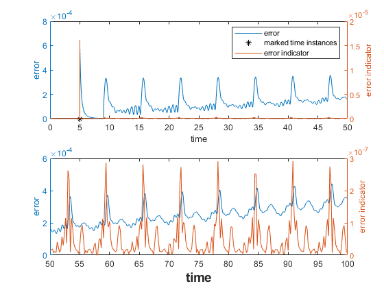
(a) $\epsilon=1.$

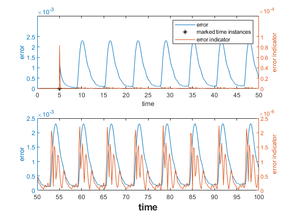
(b) $\epsilon=0.5.$

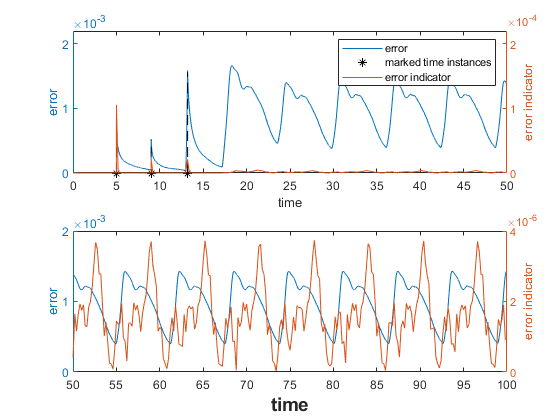
(c) $\epsilon=0.1.$

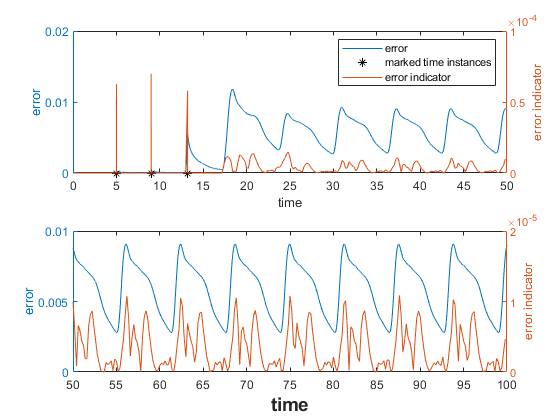
(d) $\epsilon=0.05.$

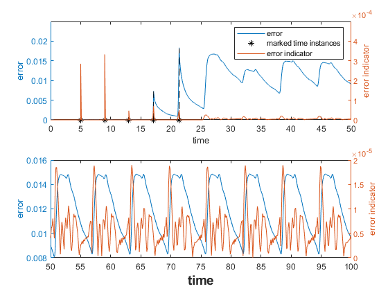
(e) $\epsilon=0.01.$

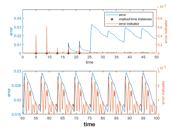
(f) $\epsilon=0.005.$

Figure 1: The evolution curves of the error indicator and the error obtined by the method Aug-APOD for solution of (4.2) with $\epsilon=1,0.5,0.1,0.05,0.01,0.005$, respectively

We then compare our method with the methods FEM, POD and TG-APOD in Table 2, where different methods are shown. The parameters set for the method TG-APOD and the method Aug-APOD are the same expect the threshold value $\eta_{0}$.

In Table 2, ‘Update Times’ means the number of updates for the POD modes in the adaptive POD methods, ‘DOFs’ means the degree of freedom, ‘Error’ denotes the relative error for numerical solution at t=T, ‘Average Error’ denotes the average of relative error for numerical approximation at each time instance on time interval $[0,T]$ and ‘Time’ means the wall time for the simulation.

From Table 2, we can first see that although the number of updates and the degrees of freedom for the POD type methods increase with the decrease of $\epsilon$, the degrees of freedom for the POD type methods for all cases of different $\epsilon$ are much smaller than those for the standard finite element method. We also see that as the decrease of $\epsilon$, the error obtained by the standard POD method increases dramatically, which makes the results unreliable when $\epsilon$ is close to zero. This show us that the smaller the $\epsilon$, the more difficult the model to be simulated. Fortunately, results obtained by the two adaptive POD methods are still of high accuracy even for case of $\epsilon=0.005$, and the CPU time cost by the adaptive POD methods is less than one-half of that used by the standard finite element method. This shows that the adaptive POD methods behave much better than the standard POD method. We now compare the two adaptive POD methods Aug-APOD and TG-APOD. We see from Table 2 that the both two methods cost similar time with the similar degrees of freedom, but the new method Aug-APOD can achieve higher accuracy, especially for cases of $\epsilon$ being very close to zero. Specifically, for cases of $\epsilon=0.01$ and $\epsilon=0.005$, our new method can achieve higher accuracy by using less POD modes and less CPU time, and its average error can even be an order of magnitude smaller than that obtained by method TG-APOD.

We have done more tests with other $\eta_{0}$ and different coarse meshes for cases of $\epsilon=0.01$ and $\epsilon=0.005$. The corresponding results are provided in “Appendix A ”.

Table 2: The results of (4.2) with different $\epsilon$ obtained by methods FEM, POD, TG-APOD and Aug-APOD, respectively

$\epsilon$	Method	$\eta_{0}$	Update Times	DOFs	Error	Average Error	Time(s)
1	FEM	-	-	10485760	-	-	15041.77
	POD	-	-	19	0.003877	0.001094	1859.07
	TG-APOD	1e-3	1	13	0.000350	0.000207	1829.59
	Aug-APOD	1e-5	1	14	0.000347	0.000184	1900.86
0.5	FEM	-	-	10485760	-	-	14772.71
	POD	-	-	22	0.002337	0.009928	1805.14
	TG-APOD	5e-3	1	15	0.001546	0.001568	1685.59
	Aug-APOD	1e-5	1	16	0.000706	0.000808	1726.65
0.1	FEM	-	-	10485760	-	-	14998.48
	POD	-	-	29	0.140401	0.223960	1943.66
	TG-APOD	1e-3	3	47	0.001719	0.001238	3154.18
	Aug-APOD	1e-5	3	48	0.001428	0.000839	3182.90
0.05	FEM	-	-	10485760	-	-	13188.19
	POD	-	-	34	0.325160	0.415044	1448.42
	TG-APOD	5e-3	3	58	0.009429	0.010761	3350.81
	Aug-APOD	5e-5	3	59	0.008989	0.005068	3288.42
0.01	FEM	-	-	16777216	-	-	11784.99
	POD	-	-	43	0.919008	0.777626	1267.46
	TG-APOD	5e-3	5	144	0.013528	0.015620	4511.11
	TG-APOD	3e-3	6	165	0.010431	0.010523	5043.79
	Aug-APOD	3e-5	5	147	0.009588	0.009403	4505.68
	Aug-APOD	1e-5	6	172	0.006208	0.003351	5280.25
0.005	FEM	-	-	16777216	-	-	12526.50
	POD	-	-	45	1.010868	0.871304	1306.83
	TG-APOD	1e-2	5	170	0.059025	0.037340	5040.39
	TG-APOD	5e-3	6	200	0.018382	0.022522	5713.98
	Aug-APOD	5e-5	5	176	0.017100	0.017024	5084.80
	Aug-APOD	3e-5	6	207	0.013551	0.008223	5913.76

To see more clearly, we show the variation curves of the error obtained by the two adaptive POD methods in Figure 2. The x-axis of each figure is the time, the y-axis is the relative error of numerical solution obtained by the adaptive POD methods. For the cases of $\epsilon=1,0.5,0.1,0.05$, the blue curve denotes the error obtained by the method Aug-APOD, and the orange curve denotes the error obtained by the method TG-APOD. For the cases of $\epsilon=0.01,0.005$, the blue curve and orange curve denote the error obtained by the method Aug-APOD with different $\eta_{0}$, respectively, and the yellow curve and purple curve denote the error obtained by the method TG-APOD with different $\eta_{0}$, respectively. If we take a detail look at the error obtained by the two methods over the entire time interval, we can find that the error obtained by our method Aug-APOD is always smaller than that obtained by the method TG-APOD. Moreover, taking into account the wall time reported in Table 2, the simulation denoted by orange curve costs the least CPU time for case of $\epsilon=0.01$. From these comparison, we can see that our new method Aug-APOD is more efficient than the method TG-APOD.

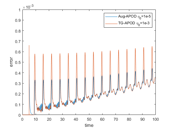
(a) $\epsilon=1.$

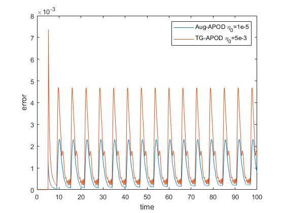
(b) $\epsilon=0.5.$

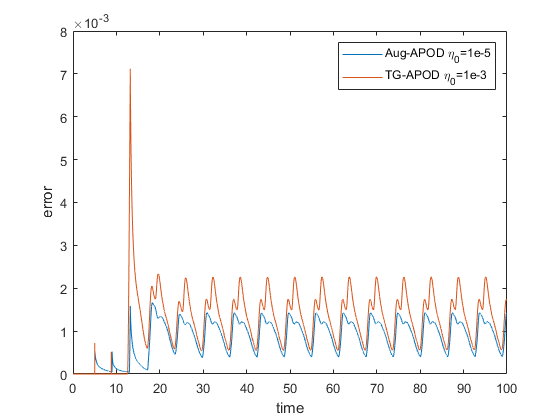
(c) $\epsilon=0.1.$

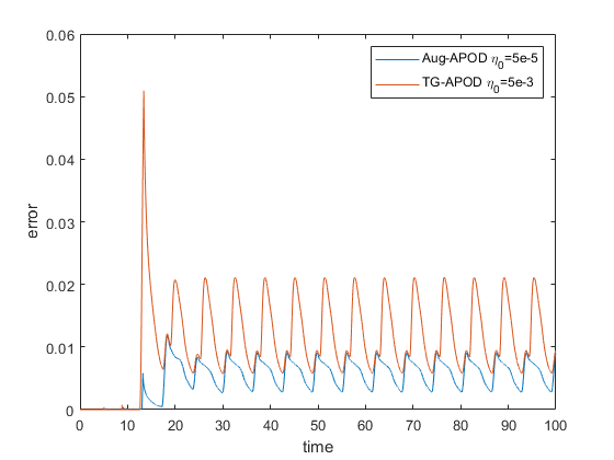
(d) $\epsilon=0.05.$

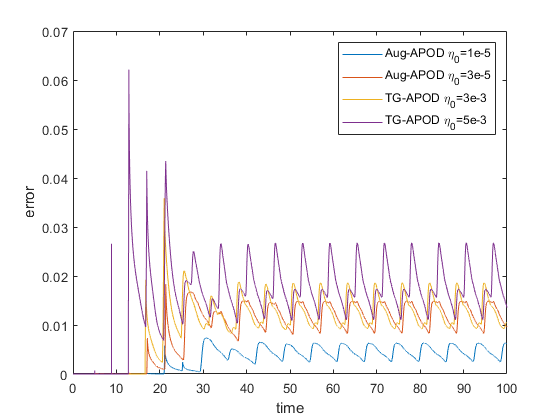
(e) $\epsilon=0.01.$

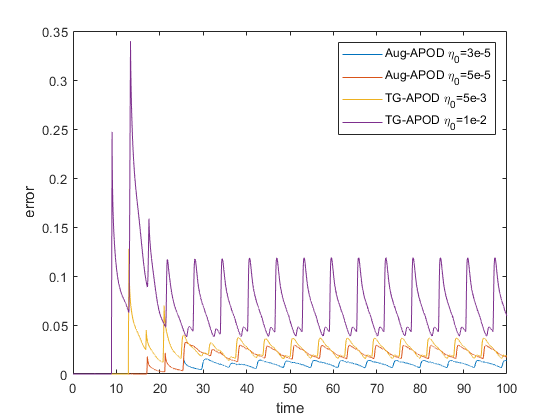
(f) $\epsilon=0.005.$

Figure 2: The evolution curves of the error for solution of (4.2) with different $\epsilon$ by methods TG-APOD and Aug-APOD, respectively

4.2 Arnold-Beltrami-Childress(ABC) flow

We then consider another advection-diffusion equations with the advection being the ABC flow, which plays an important role in fluid dynamics [16; 58; 8].

$$\left\{\begin{aligned} &u_{t}-\epsilon\Delta u+{\bf B}(x,y,z,t)\cdot\nabla u=f(x,y,z,t),\quad(x,y,z)\in\Omega,t\in[0,T],\\ &u(x,y,z,0)=0,\\ &u(x+2\pi,y,z,t)=u(x,y+2\pi,z,t)=u(x,y,z+2\pi,t)=u(x,y,z,t),\end{aligned}\right.$$ (4.3)

where

$${\bf B}(x,y,z,t)= (\sin(z+\sin wt)+\cos(y+\sin wt),\sin(x+\sin wt)$$

$$+\cos(z+\sin wt),\sin(y+\sin wt)+\cos(x+\sin wt)),$$

$$f(x,y,z,t)= -\sin(z+\sin wt)-\cos(y+\sin wt),$$

$$\Omega=[0,2\pi]^{3}, T=100.$$

For this example, we also test 6 different cases with $\epsilon=1,0.5,0.1,0.05,0.01,0.005$, respectively.

Similar to the example of Kolmogorov flow, we first divide the $\Omega$ into 6 tetrahedrons to act as the initial mesh. Then we refine the initial mesh 23 times uniformly using bisection to obtain the fine mesh for cases of $\epsilon=1,0.5,0.1,0.05$, and refine the initial mesh 24 times to obtain the fine mesh for cases of $\epsilon=0.01,0.005$. We set $w=1.0$, $\delta t=5\times 10^{-3}$ and choose the piecewise linear function as the finite element basis. For the POD type methods, we choose the same parameters as those for solving (4.2) expect the coarse meshes used by the two adaptive POD methods. We refine the initial mesh 14 times to obtain the coarse mesh for cases of $\epsilon=1,0.5,0.1$, and refine the initial mesh 15 times to obtain the coarse mesh for cases of $\epsilon=0.05,0.01,0.005$. The time steps corresponding to the coarse finite element spaces are 0.2 and 0.125, respectively. We use the similar number of processors as those for the Kolmogorov flow to do the simulation, that is, we use 72 processors and 180 processors for cases of the fine mesh being obtained by refining the initial mesh 23 times and 24 times, respectively.

Similarly, we show the error and the error indicator obtained by our method Aug-APOD in Figure 3. The x-axis and y-axis of each sub-figure have the same meaning as those in Figure 1. In each sub-figure, the blue curve and orange curve also describe the variation of the error and error indicator, and the black star also denotes the marked time instance. Figure 3 shows that the variation of the error indicator is proportional to that of the error. This means that the error indicator is also very effective for this example.

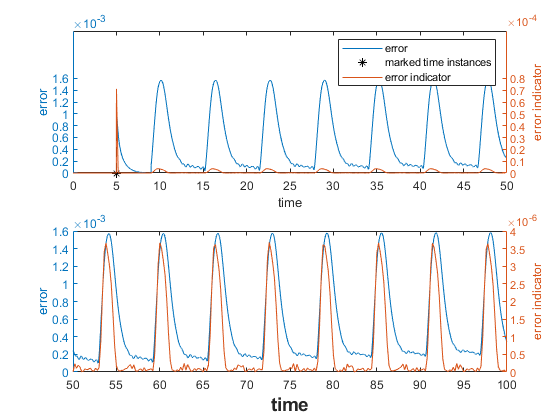
(a) $\epsilon=1.$

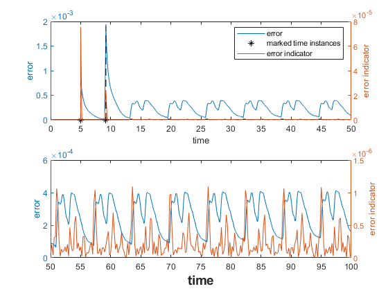
(b) $\epsilon=0.5.$

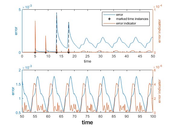
(c) $\epsilon=0.1.$

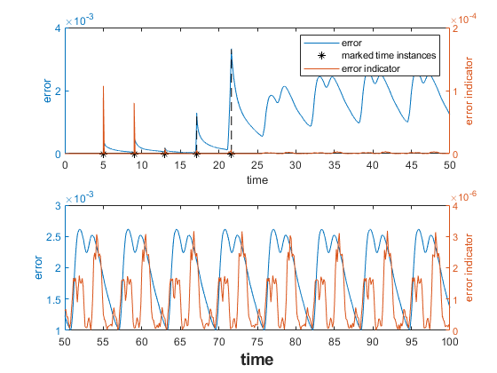
(d) $\epsilon=0.05.$

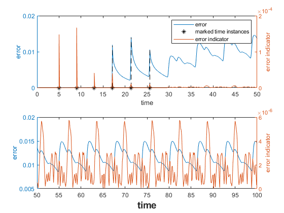
(e) $\epsilon=0.01.$

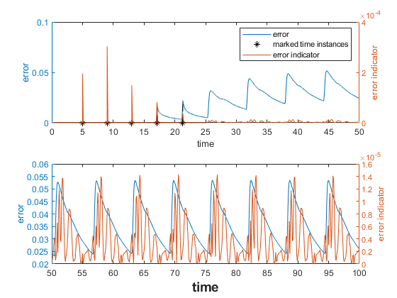
(f) $\epsilon=0.005.$

Figure 3: The evolution curves of the error indicator and the error obtined by the method Aug-APOD for solution of (4.3) with $\epsilon=1,0.5,0.1,0.05,0.01,0.005$, respectively

The numerical results obtained by methods FEM, POD, TG-APOD and Aug-APOD are shown in Table 3. The parameters set for the methods TG-APOD and Aug-APOD are the same expect the threshold value $\eta_{0}$. The notation in Table 3 has the same meaning as those in Table 2.

Similar to the first example, from Table 3, we see that the POD type methods save much CPU time. The results obtained by the standard POD method are also unreliable as the decrease of $\epsilon$. The two adaptive POD methods are also of high accuracy even for case of $\epsilon=0.005$. Moreover, the adaptive POD methods can save approximately two-thirds of the CPU time compared with that cost by the standard finite element method. This shows that the two adaptive POD methods behave much better than the standard POD method. For the two adaptive POD methods Aug-APOD and TG-APOD, our new method Aug-APOD behaves better than the method TG-APOD. Specifically, the method Aug-APOD can achieve higher accuracy with similar number of POD modes for cases of $\epsilon=0.05,0.01,0.005$. Moreover, for case of $\epsilon=0.005$, the method Aug-APOD can use less CPU time to obtain results as accurate as those obtained by the method TG-APOD.

Similarly, more numerical results obtained by using other $\eta_{0}$ and different coarse meshes for case of $\epsilon=0.005$ can be found in “Appendix A ”.

Table 3: The results of (4.3) with different $\epsilon$ obtained by methods FEM, POD, TG-APOD and Aug-APOD, respectively

$\epsilon$	Method	$\eta_{0}$	Update Times	DOFs	Error	Average Error	Time(s)
1	FEM	-	-	10485760	-	-	20427.20
	POD	-	-	24	0.000974	0.013559	1681.67
	TG-APOD	3e-3	1	17	0.000335	0.000517	2304.13
	Aug-APOD	5e-6	1	17	0.000341	0.000522	2340.55
0.5	FEM	-	-	10485760	-	-	18432.76
	POD	-	-	26	0.007569	0.069137	1625.80
	TG-APOD	1e-3	2	28	0.000145	0.000234	3044.43
	Aug-APOD	5e-6	2	28	0.000154	0.000244	3064.83
0.1	FEM	-	-	10485760	-	-	17362.39
	POD	-	-	35	0.136214	0.373726	1727.87
	TG-APOD	1e-3	4	68	0.001716	0.001258	4940.78
	Aug-APOD	5e-6	4	67	0.001767	0.000998	4889.35
0.05	FEM	-	-	10485760	-	-	17391.44
	POD	-	-	40	0.257052	0.514289	1814.08
	TG-APOD	3e-3	5	100	0.003220	0.002760	6209.27
	Aug-APOD	5e-6	5	99	0.001352	0.001507	6222.50
0.01	FEM	-	-	16777216	-	-	16065.81
	POD	-	-	44	0.577333	0.697981	1515.37
	TG-APOD	8e-3	5	166	0.026295	0.022662	5796.19
	TG-APOD	3e-3	6	192	0.015234	0.012518	6640.86
	Aug-APOD	1e-5	5	164	0.015639	0.016240	6037.70
	Aug-APOD	8e-6	6	193	0.014533	0.008428	6808.99
0.005	FEM	-	-	16777216	-	-	16836.62
	POD	-	-	44	0.812194	0.836567	1554.84
	TG-APOD	1e-2	5	194	0.046166	0.039155	6437.76
	TG-APOD	5e-3	6	226	0.027286	0.023730	7147.38
	Aug-APOD	3e-5	5	193	0.027987	0.027651	6592.85
	Aug-APOD	1e-5	5	192	0.026378	0.027074	6517.28

Similar to the first example, we show the comparison between the methods TG-APOD and Aug-APOD in Figure 4. The x-axis of each figure is the time, the y-axis is the relative error of numerical solution obtained by the adaptive POD methods. It is obvious that the error obtained by the method Aug-APOD is smaller than that obtained by the method TG-APOD over the entire time interval for cases of $\epsilon=0.05$ and $\epsilon=0.01$. From these comparison, we can also see that our new method Aug-APOD behaves better than the method TG-APOD.

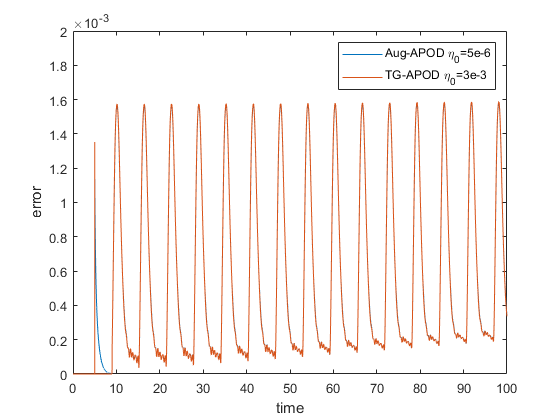
(a) $\epsilon=1.$

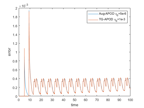
(b) $\epsilon=0.5.$

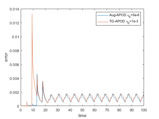
(c) $\epsilon=0.1.$

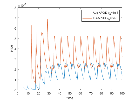
(d) $\epsilon=0.05.$

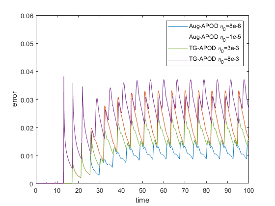
(e) $\epsilon=0.01.$

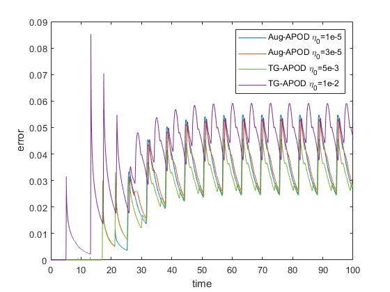
(f) $\epsilon=0.005.$

Figure 4: The evolution curves of the error for solution of (4.3) with different $\epsilon$ by methods TG-APOD and Aug-APOD, respectively

From the two examples we have tested, we see that our new method Aug-APOD has better performance than the exiting methods.

5 Concluding remarks

In this paper, we have proposed a new approach for adaptive POD methods to solve time dependent partial differential equations efficiently and accurately. By augmenting the POD subspace with some auxiliary modes, we have obtained an augmented subspace. We have used the difference between the approximation obtained in this augmented subspace and that obtained in the original POD subspace to construct an error indicator. Using this idea, we have obtained a general framework for the augmented subspace based adaptive POD method. We have then provided two specific methods to obtain the auxiliary mode, one is generating vector randomly, the other is computing the coarse-grid approximations.

We have compared the new approach with the two-grid based adaptive method to test two typical 3D advection-diffusion equations, including both cases with the advection being the Kolmogorov flow and the ABC flow. Numerical results show that our method is more efficient than the existing adaptive methods, especially for cases of $\epsilon=0.01,0.005$. In our future work, we will pay more effort on applying the method to other types of time dependent partial differential equations and constructing other effective error indicators.

Appendix A Numerical experiments for different coarse meshes and different $\eta_{0}$

In this section, we use more numerical experiments to illustrate that our new method performs better than the two-grid based adaptive POD method, especially for cases of $\epsilon=0.01,0.005$. We denote the two-grid based adaptive POD method and our augmented subspace based adaptive POD method with the coarse grid obtained by refining the initial mesh $N$ times as TG-APOD-$N$ and Aug-APOD-$N$, respectively. The time steps corresponding to different coarse finite spaces are listed in Table 4. With a fixed fine grid, we have tested (4.2) with $\epsilon=0.01,0.005$ and (4.3) with $\epsilon=0.005$ by different coarse meshes and different threshold $\eta_{0}$, respectively.

Table 4: Time steps corresponding to different coarse meshes

$N$-Refine	14	15	16	17
Time step	0.2	0.125	0.1	0.05

A.1 Kolmogorov flow with $\epsilon=0.01$

The results of (4.2) with $\epsilon=0.01$ obtained by different methods and different parameters are shown in Table 5. From Table 5, we can draw the similar conclusion as those from Table 2. We first see that all adaptive POD methods can obtain results with some accuracy when compared with those obtained by the FEM method but cost much less CPU time than the FEM method. Then, we see that all adaptive POD methods behave much better than the traditional POD method. With similar number of POD modes, the results obtained by our augmented subspace based adaptive POD method are more accurate than those obtained by other POD type methods.

Table 5: The results of (4.2) with $\epsilon=0.01$ obtained by different POD type methods with different coarse meshes and $\eta_{0}$, respectively

$\epsilon$	Method	$\eta_{0}$	Update Times	DOFs	Error	Average Error	Time(s)
0.01	FEM	-	-	16777216	-	-	11784.99
	POD	-	-	43	0.919008	0.777626	1267.46
	TG-APOD-14	5e-3	5	143	0.024535	0.029794	4424.10
	TG-APOD-14	3e-3	5	144	0.013786	0.017077	4522.11
	TG-APOD-14	1e-3	6	167	0.009079	0.011065	5180.53
	TG-APOD-15	5e-3	5	144	0.013528	0.015620	4511.11
	TG-APOD-15	3e-3	6	165	0.010431	0.010523	5043.79
	TG-APOD-15	1e-3	6	166	0.007042	0.004837	5072.23
	TG-APOD-16	5e-3	5	147	0.011280	0.012568	4602.02
	TG-APOD-16	3e-3	6	170	0.007904	0.008971	5130.71
	TG-APOD-16	1e-3	7	196	0.005060	0.003834	5789.31
	Aug-APOD-14	5e-5	5	149	0.022220	0.015238	4453.28
	Aug-APOD-14	3e-5	5	148	0.019160	0.016858	4410.95
	Aug-APOD-14	1e-5	6	173	0.008892	0.004957	5302.05
	Aug-APOD-14	5e-6	7	199	0.001541	0.001740	5708.77
	Aug-APOD-15	5e-5	5	147	0.009849	0.009620	4560.84
	Aug-APOD-15	3e-5	5	147	0.009588	0.009403	4505.68
	Aug-APOD-15	1e-5	6	172	0.006208	0.003351	5280.25
	Aug-APOD-15	5e-6	7	199	0.003427	0.001915	5996.87
	Aug-APOD-16	5e-5	5	147	0.008976	0.009054	4557.52
	Aug-APOD-16	3e-5	5	147	0.008976	0.009054	4505.68
	Aug-APOD-16	1e-5	6	172	0.006253	0.003377	5335.85

A.2 Kolmogorov flow with $\epsilon=0.005$

We show the results of (4.2) with $\epsilon=0.005$ obtained by different methods and different parameters in Table 6. For this case of $\epsilon$, we can also draw the similar conclusion as those from Table 2 and Table 5, that is, our augmented subspace based adaptive POD method behave better than other methods.

Table 6: The results of (4.2) with $\epsilon=0.005$ obtained by different POD type methods with different coarse meshes and $\eta_{0}$, respectively

$\epsilon$	Method	$\eta_{0}$	Update Times	DOFs	Error	Average Error	Time(s)
0.005	FEM	-	-	16777216	-	-	12526.50
	POD	-	-	45	1.010868	0.871304	1306.83
	TG-APOD-14	1e-2	4	139	0.110962	0.091636	4132.52
	TG-APOD-14	5e-3	5	171	0.062622	0.073958	4950.07
	TG-APOD-15	1e-2	5	170	0.059025	0.037340	5040.39
	TG-APOD-15	5e-3	6	200	0.018382	0.022522	5713.98
	TG-APOD-16	1e-2	5	178	0.023319	0.022661	5181.44
	TG-APOD-16	5e-3	6	208	0.015640	0.014779	5887.37
	Aug-APOD-14	5e-5	5	176	0.018007	0.018023	4893.47
	Aug-APOD-14	3e-5	6	206	0.013928	0.008509	5789.30
	Aug-APOD-14	1e-5	6	207	0.014098	0.007749	5696.05
	Aug-APOD-15	5e-5	5	176	0.017100	0.017024	5084.80
	Aug-APOD-15	3e-5	6	207	0.013551	0.008223	5913.76
	Aug-APOD-15	1e-5	7	239	0.008122	0.004791	6891.73
	Aug-APOD-16	5e-5	5	176	0.017162	0.016912	5295.97
	Aug-APOD-16	3e-5	5	176	0.017162	0.016912	5149.72
	Aug-APOD-16	1e-5	7	239	0.007957	0.004724	6778.84

A.3 ABC flow with $\epsilon=0.005$

In Table 7, we show the results of (4.3) with $\epsilon=0.005$ obtained by different methods and different parameters. Similar to the example of Kolmogorov flow, the adaptive POD methods behave better than other methods, and our augmented subspace based adaptive POD method behave better than the two-grid based adaptive POD method.

Table 7: The results of (4.3) with $\epsilon=0.005$ obtained by different POD type methods with different coarse meshes and $\eta_{0}$, respectively

$\epsilon$	Method	$\eta_{0}$	Update Times	DOFs	Error	Average Error	Times
0.005	FEM	-	-	16777216	-	-	16836.62
	POD	-	-	44	0.812194	0.836567	1554.84
	TG-APOD-15	1e-2	5	194	0.046166	0.039155	6437.76
	TG-APOD-15	5e-3	6	226	0.027286	0.023730	7147.38
	TG-APOD-16	2e-2	5	198	0.086156	0.076253	6563.74
	TG-APOD-16	1e-2	6	228	0.034736	0.035273	7395.12
	TG-APOD-16	5e-3	7	259	0.025176	0.020051	8409.76
	TG-APOD-17	2e-2	5	195	0.046125	0.038615	6460.26
	TG-APOD-17	1e-2	8	294	0.025939	0.019266	9540.73
	TG-APOD-17	5e-3	9	323	0.017107	0.010361	10735.34
	Aug-APOD-15	5e-5	4	159	0.065712	0.051971	5581.35
	Aug-APOD-15	3e-5	5	193	0.027987	0.027651	6592.85
	Aug-APOD-15	2e-5	5	193	0.027987	0.027651	6480.75
	Aug-APOD-15	1e-5	5	192	0.026378	0.027074	6517.28
	Aug-APOD-16	5e-5	5	192	0.032155	0.031447	6468.33
	Aug-APOD-16	3e-5	5	192	0.025921	0.026135	6512.32
	Aug-APOD-16	2e-5	5	192	0.025921	0.026135	6479.52
	Aug-APOD-16	1e-5	9	323	0.011047	0.014037	10392.84

References

- [1] R. A. Adams. Sobolev Spaces. New York: Academic Press, 1975.
- [2] M. Bakker. Simple Groundwater Flow Models for Seawater Intrusion. Proceedings of SWIM16, WolinIsland, Poland., pages 180–182, 2000.
- [3] G. K. Batchelor. An Introduction to Fluid Dynamics. Cambridge University Press, Cambridge, 2 edition, 1999.
- [4] P. Benner, S. Gugercin, and K. Willcox. A Survey of Projection-Based Model Reduction Methods for Parametric Dynamical Systems. SIAM Rev., 57(4):483–531, 2015.
- [5] V. Borue and O. Sa. Numerical Study of Three-Dimensional Kolmogorov Flow at High Reynolds Numbers. J. Fluid Mech., 306:293–323, 1996.
- [6] S. Boyaval, C. Le Bris, T. Lelievre, Y. Maday, N. C. Nguyen, and A. T. Patera. Reduced Basis Techniques for Stochastic Problems. Arch. Comput. Methods Eng., 17(4):435–454, 2010.
- [7] S. Brenner and L. Scott. The Mathematical Theory of Finite Element Methods. Springer, New York, 3 edition, 2008.
- [8] N. H. Brummell, F. Cattaneo, and S. M. Tobias. Linear and Nonlinear Dynamo Properties of Time-Dependent ABC Flows. Fluid Dyn. Res., 28(4):237–265, 2001.
- [9] J. Burkardt, M. Gunzburger, and H. C. Lee. POD and CVT-Based Reduced-Order Modeling of Navier-Stokes Flows. Comput. Methods Appl. Mech. and Eng., 196(1-3):337–355, 2006.
- [10] J. R. Cannon. The One-Dimensional Heat Equation. Addison-Wesley, Mento Park, 1984.
- [11] F. Chinesta, A. Huerta, G. Rozza, and K. Willcox. Model Reduction Methods. Encyclopedia of Computational Mechanics Second Edition., pages 1–36, 2017.
- [12] X. Dai, X. Kuang, Z. Liu, J. Xin, and A. Zhou. An Adaptive Proper Orthogonal Decomposition Galerkin Method for Time Dependent Problems. preprint, 2017.
- [13] X. Dai, X. Kuang, J. Xin, and A. Zhou. Two-Grid Based Adaptive Proper Orthogonal Decomposition Method for Time Dependent Partial Differential Equations. J. Sci. Comput., 84(3):Paper No. 47, 27 pp., 2020.
- [14] X. Dai, J. Xu, and A. Zhou. Convergence and Optimal Complexity of Adaptive Finite Element Eigenvalue Computations. Numer. Math., 110(3):313–355, 2008.
- [15] B. T. Dickinson and J. R. Singler. Nonlinear Model Reduction Using Group Proper Orthogonal Decomposition. Int. J. Numer. Anal. Model., 7(2):356–372, 2010.
- [16] T. Dombre, U. Frisch, J. M. Greene, M. Hnon, A. Mehr, and A. M. Soward. Chaotic Streamlines in the ABC Flows. J. Fluid Mech., 167:353–391, 1986.
- [17] P. Druault, J. Delville, and J. P. Bonnet. Proper Orthogonal Decomposition of the Mixing Layer Flow Into Coherent Structures and Turbulent Gaussian Fluctuations. C. R. Mcanique, 333(11):824–829, 2005.
- [18] G. H. Golub and C. F. van Loan. Matrix Computations. JHU Press, fourth edition, 2013.
- [19] C. Gräßle and M. Hinze. POD Reduced-Order Modeling for Evolution Equations Utilizing Arbitrary Finite Element Discretizations. Adv. Comput. Math., 44(6):1941–1978, 2018.
- [20] A. Gu, J. Xin, and Z. Zhang. Error Estimates for a POD Method for Solving Viscous G-Equation in Incompressible Cellular Flows. SIAM J. Sci. Comput., 43(1):A636–A662, 2021.
- [21] Y. He. The Euler Implicit/Explicit Scheme for the 2D Time-Dependent Navier-Stokes Equations with Smooth or Non-Smooth Initial Data. Math. Comput., 77(264):2097–2124, 2008.
- [22] J. S. Hesthaven, G. Rozza, and B. Stamm. Certified Reduced Basis Methods for Parametrized Partial Differential Equations, volume 590. Springer, 2016.
- [23] P. Holmes, J. L. Lumley, and G. Berkooz. Turbulence, Coherent Structures, Dynamical Systems and Symmetry. Cambridge University Press, Cambridge, 1996.
- [24] C. Homescu, L. R. Petzold, and R. Serban. Error Estimation for Reduced-Order Models of Dynamical Systems. SIAM J. Numer. Anal., 43(4):1693–1714, 2005.
- [25] T. Katayama, H. Kawauchi, and G. Picci. Subspace Identification of Closed Loop Systems by the Orthogonal Decomposition Method. Automatica, 41(5):863–872, 2005.
- [26] M. Khalil, S. Adhikari, and A. Sarkar. Linear System Identification Using Proper Orthogonal Decomposition. Mech. Syst. Signal Process., 21(8):3123–3145, 2007.
- [27] B. Koc, S. Rubino, M. Schneier, J. Singler, and T. Iliescu. On Optimal Pointwise in Time Error Bounds and Difference Quotients for the Proper Orthogonal Decomposition. SIAM J. Numer. Anal., 59(4):2163–2196, 2021.
- [28] D. Kosloff and R. Kosloff. A Fourier Method Solution for the Time Dependent Schrodinger Equation as a Tool in Molecular Dynamics. J. Comput. Phys., 52(1):35–53, 1983.
- [29] K. Kunisch and S. Volkwein. Galerkin Proper Orthogonal Decomposition Methods for Parabolic Problems. Numer. Math., 90(1):117–148, 2001.
- [30] K. Kunisch and S. Volkwein. Galerkin Proper Orthogonal Decomposition Methods for a General Equation in Fluid Dynamics. SIAM J. Numer. Anal., 40(2):492–515, 2002.
- [31] K. Kunisch and S. Volkwein. Optimal Snapshot Location for Computing POD Basis Functions. ESAIM: Math. Model. Numer. Anal., 44(3):509–529, 2010.
- [32] H. Li and Z. Song. A Reduced-Order Finite Element Method Based on Proper Orthogonal Decomposition for the Allen-Cahn Model. J. Math. Anal. Appl., 500(2):125103, 2021.
- [33] K. Li, T. Huang, L. Li, and S. Lanteri. Pod-Based Model Order Reduction with an Adaptive Snapshot Selection for a Discontinuous Galerkin Approximation of the Time-Domain Maxwell’s Equations. J. Comput. Phys., 396:106–128, 2019.
- [34] S. Locke and J. Singler. New Proper Orthogonal Decomposition Approximation Theory for PDE Solution Data. SIAM J. Numer. Anal., 58(6):3251–3285, 2020.
- [35] H.V. Ly and H.T. Tran. Modeling and Control of Physical Processes Using Proper Orthogonal Decomposition. Math. Comput. Modell., 33(1-3):223–236, 2001.
- [36] J. Lyu, Z. Wang, J. Xin, and Z. Zhang. A Convergent Interaction Particle Method and Computation of KPP Front Speeds in Chaotic Flows. SAIM J. Numer. Anal., 60(3):1136–1167, 2022.
- [37] J. Lyu, J. Xin, and Y. Yu. Computing Residual Diffusivity by Adaptive Basis Learning via Spectral Method. Numer. Math. Theory Methods Appl., 10(2):351–372, 2017.
- [38] Y. Maday. Reduced Basis Method for the Rapid and Reliable Solution of Partial Differential Equations. In Proceedings of International Conference of Mathematicians, pages 1255–1270, European Mathematical Society, volume III, 2006.
- [39] P. A. Markowych, C. A. Ringhofer, and C. Schmeiser. Semiconductor Equations. Springer, Vienna, 1990.
- [40] J. Nolen, M. Rudd, and J. Xin. Existence of KPP Fronts in Spatially-Temporally Periodic Advection and Variational Principle for Propagation Speeds. Dynam. Part. Differ. Eq., 2(1):1–24, 2005.
- [41] A. M. Obukhov. Kolmogorov Flow and Its Laboratory Simulation. Rus. Uspekhi Mat. Nauk., 38(4):101–111, 1983.
- [42] R. Padhi and S. N. Balakrishnan. Proper Orthogonal Decomposition Based Optimal Neurocontrol Synthesis of a Chemical Reactor Process Using Approximate Dynamic Programming. Neural Netw., 16(5):719–728, 2003.
- [43] B. Peherstorfer and K. Willcox. Dynamic Data-Driven Reduced-Order Models. Comput. Methods Appl. Mech. Eng., 291:21–41, 2015.
- [44] PETSc. http:// www.mcs.anl.gov/petsc/.
- [45] PHG. http://lsec.cc.ac.cn/phg/.
- [46] R. Pinnau. Model Reduction via Proper Orthogonal Decomposition. In: Model Order Reduction: Theory, Research Aspects and Applications. Springer, Berlin, Heidelberg, 2008.
- [47] A. Quarteroni and G. Rozza. Reduced Order Methods for Modeling and Computational Reduction, volume 9. Springer, Berlin, 2014.
- [48] M. L. Rapn, F. Terragni, and J. M. Vega. Adaptive POD-Based Low-Dimensional Modeling Supported by Residual Estimates. Int. J. Numer. Methods Eng., 104(9):844–868, 2015.
- [49] C. Rowley, T. Colonius, and R. Murray. Model Reduction for Compressible Flows Using POD and Galerkin Projection. Phys. D, 189(1-2):115–129, 2004.
- [50] Y. Saad and M. Schultz. GMRES: A Generalized Minimal Residual Algorithm for Solving Nonsymmetric Linear Systems. SIAM J. Sci. Stat. Comput., 7:856–869, 1986.
- [51] L. Sirovich. Turbulence and the Dynamics of Coherent Structures. Part I: Coherent Structures. Q. Appl. Math., 45(3):561–571, 1987.
- [52] J. Strikwerda. Finite Difference Schemes and Partial Differential Equations. SIAM, Philadelphia, 2004.
- [53] M. V. Tabib and J. B. Joshi. Analysis of Dominant Flow Structures and Their Flow Dynamics in Chemical Process Equipment Using Snapshot Proper Orthogonal Decomposition Technique. Chem. Eng. Sci., 63(14):3695–3715, 2008.
- [54] F. Terragni and J. M. Vega. Simulation of Complex Dynamics Using Pod ‘On the Fly’ and Residual Estimates. In : Dynamical systems, Differential Equations and Applications AIMS Proceedings., pages 1060–1069, 2015.
- [55] S. Volkwein. Model Reduction Using Proper Orthogonal Decomposition. Lecture Notes, Institute of Mathematics and Scientific Computing, Universityof Graz., 1025, 2011.
- [56] S. Volkwein. Proper Orthogonal Decomposition: Theory and Reduced-Order Modelling. Lecture Notes, Department of Mathematics and Statistics, University of Konstanz, 2013.
- [57] Z. Wang, J. Xin, and Z. Zhang. Sharp Uniform in Time Error Estimate on a Stochastic Structure-Preserving Lagrangian Method and Computation of Effective Diffusivity in 3D Chaotic Flows. SIAM Multiscale Model. Simul., 19:1167–1189, 2021.
- [58] J. Xin, Y. Yu, and A. Zlatos. Periodic Orbits of the ABC Flow with A = B = C = 1. SIAM J. Math. Anal., 48(6):4087–4093, 2016.
- [59] C. Xu, Y. Ou, and E. Schuster. Sequential Linear Quadratic Control of Bilinear Parabolic PDEs Based on POD Model Reduction. Automatica, 47(2):418–426, 2011.
- [60] P. Zu, L. Chen, and J. Xin. A Computational Study of Residual App Front Speeds in Time-Periodic Cellular Flows in the Small Diffusion Limit. Physica D, 311:37–44, 2015.