Polytopes of Absolutely Wigner Bounded Spin States

Abstract

We study the properties of unitary orbits of mixed spin states that are characterized by Wigner functions lower bounded by a specified value. To this end, we extend a characterization of the set of absolutely Wigner positive states as a set of linear eigenvalue constraints, which together define a polytope in the simplex of spin-$j$ mixed states centred on the maximally mixed state. The lower bound determines the relative size of such absolutely Wigner bounded (AWB) polytopes and we study their geometric properties. In particular, in each dimension a Hilbert-Schmidt ball representing a tight AWB sufficiency criterion based on the purity is exactly determined, while another ball representing AWB necessity is conjectured. Special attention is given to the case where the polytope separates orbits containing only positive Wigner functions from other orbits because of the use of Wigner negativity as a witness of non-classicality of spin states. Comparisons are made to absolute symmetric state separability and spherical Glauber-Sudarshan positivity, with additional details given for low spin quantum numbers.

1 Introduction

Negative quasiprobability in the phase space representation has long been an indicator of non-classicality in quantum systems. The three most studied types of quasiprobability are those associated with the Wigner function, the Glauber-Sudarshan function, and the Kirkwood-Dirac function, particularly so in recent years due to the rise of quantum information theory. Wigner negativity in particular has received special attention because of its relationship to quantum advantage in the magic state injection model of universal fault-tolerant quantum computation [1, 2, 3, 4, 5]. In this setting Wigner negativity acts as a magic monotone with respect to Gaussian/Clifford group operations, and so offers some credence to the idea that more negativity implies more non-classicality [6, 7, 8].

For pure states in bosonic systems the set of Wigner-positive states is fully characterized by Hudson’s theorem, be it Gaussian states in the continuous variable regime or stabilizer states in the discrete variable regime [9, 10]. However the relationship between negative quasiprobability and state mixedness is not well understood. For both practical and theoretical reasons this relationship is important. In the mixed bosonic setting, Gaussianity is no longer necessary to infer Wigner function positivity and the situation becomes more complicated [11, 12, 13]. A general observation is that negativity tends to decrease as purity decreases. This may be attributed to the point-wise convexity of Wigner functions over state decompositions, together with the maximally mixed state guaranteed to be Wigner-positive (at least in a limiting sense of increasingly flatter Gaussians), although the precise relationship is not fully understood. Even less understood is how Wigner negativity manifests in spin-$j$ systems, equivalent to the symmetric subspace of $2j$ qubits, which have a Moyal representation on a spherical phase space [14, 15, 16, 17, 18, 19]. Evidence suggests that no pure spin state is completely Wigner-positive [20], and the question of mixed spin states remains largely unexplored.

Inspired by work on characterizing mixed spin state entanglement in the symmetrized multi-qubit picture, in particular that of absolute separability [21, 22], here we address the question of Wigner positivity by investigating unitary orbits of spin states. The unitary orbit of a spin-$j$ state $\rho$ is defined as the set of states $\{U\rho{U^{\dagger}}:U\in\text{SU}(2j+1)\}$. In particular, we call a general spin state absolutely Wigner-positive (AWP) if its spherical Wigner function remains positive under the action of all global unitaries $U\in\text{SU}(2j+1)$.

In order to position our work in a wider context, we begin with a brief note on related research. Recent works have studied the sets of AWP states [23, 24, 25, 26] taking a broad perspective on the Moyal picture in finite dimensions by simultaneously considering the set of all candidate SU($N$)-covariant Wigner functions for each dimension $N$. It is in this general setting where the relationship between generalized Moyal theory, the existence of Wigner-positive polytopes, and the Birkoff-von Neumann theorem was first established. It was furthermore abstractly demonstrated that there always exists a compatible reduction to an appropriate $N$-dimensional SU($2$) symbol correspondence on the sphere.

By contrast, here we work exclusively with the symmetry group SU(2) in each dimension, as well as a single concrete Wigner function, Eq. (2), which we consider to be the canonical Wigner function for spin systems because it is the only SU(2)-covariant Wigner function to satisfy, in addition to the usual Stratonovich-Weyl axioms, either of the following two properties:

• Compatibility with the spherical $s$-ordered class of functions: it is exactly “in between” the Husimi $Q$ function and the Glauber-Sudarshan $P$ function (as generated by the standard spin-coherent state ${|{j,j}\rangle}$) [15].

• Compatibility with Heisenberg-Weyl symmetry: its infinite-spin limit is the original Wigner function on $\mathbb{R}^{2}$ [27].

In addition to offering a related but alternative argument showing the existence of such polytopes, here we go beyond previous investigations in three ways. The first is that we extend the argument to include orbits of Wigner functions lower-bounded by numbers not necessarily zero. These one-parameter families of polytopes, which we refer to as absolutely Wigner bounded (AWB) polytopes, are of interest not only for Wigner functions but also for other quasiprobability distributions. The second is that we go into explicit detail on the geometric properties of these polytopes and explore their relevance in the context of spin systems and quantum information. The third is that we contrast the Wigner negativity structure to the Glauber-Sudarshan negativity structure, which amounts to an accessible comparison between Wigner negativity and entanglement in the mixed state setting.

Having established the context for this work with the above description, our first result is the complete characterization of the set of AWB spin states in all finite dimensions, with AWP states appearing as a special case. As similarly discussed in [25], this may be phrased as a natural application of the Birkhoff-von Neumann theorem on doubly stochastic matrices, though here we extend and specialize to the SU(2)-covariant Wigner kernel associated with the canonical Wigner function on the sphere. In particular, the set of AWB states forms a polytope in the simplex of density matrix spectra, the $(2j+1)!$ hyperplane boundaries of which are defined by permutations of the eigenvalues of the phase-point operators. Centred on the maximally mixed state for each dimension, we also exactly find the largest possible Hilbert-Schmidt ball containing nothing but AWB states, which amounts to the strictest AWB sufficiency criterion based solely on the purity of mixed states. We also obtain an expression that we conjecture describes the smallest Hilbert-Schmidt ball containing all AWB states, which amounts to a tight necessity criterion. Numerical evidence supports this conjecture. For both criteria, we discuss their geometric interpretation in relation to the full AWB polytope. We then specialize to absolute Wigner positivity and compare it with symmetric absolute separability (SAS), which in the case of a single spin-$j$ system is equivalent to absolute Glauber-Sudarshan positivity [28, 29, 30].

Our paper is organized as follows. Section 2 briefly outlines the generalized phase space picture using the parity-operator/Stratonovich framework for the group SU(2). Section 3 proves our first result on AWB polytopes, while Sec. 4 determines and conjectures, respectively, the largest and smallest Hilbert-Schmidt ball sitting inside and outside the AWB polytopes. Section 5 explores low-dimensional cases in more detail and draws comparisons to entanglement. Finally, conclusions are drawn and perspectives are outlined in Sec. 6.

2 Background

The parity-operator framework is the generalization of Moyal quantum mechanics to physical systems other than a collection of non-relativistic spinless particles. Each type of system has a different phase space, and the various types are classified by the system’s dynamical symmetry group [31]. In each case the central object is a map, $\Delta$, called the kernel, which takes points in phase space to operators on Hilbert space. A quasi-probability representation of a quantum state, evaluated at a point in phase space, is the expectation value of the phase-point operator assigned to that point. Different kernels yield different distributions but all must obey the Stratonovich-Weyl axioms, which ensure, among other properties, the existence of an inverse map and that the Moyal picture is as close as possible to classical statistical physics over the same phase space (i.e. the Born rule as an $L^{2}$ inner product).

When applied to the Heisenberg-Weyl group (i.e. the group of displacement operators generated by the canonical commutation relations, $[x,p]=i\mathbb{1}$) this framework reduces to the common phase space associated with $n$ canonical degrees of freedom, $\mathbb{R}^{2n}$, and the phase-point operators corresponding to the Wigner function appear as a set of displaced parity operators [31, 32, 33]. A spin-$j$ system on the other hand corresponds to the group SU(2), which yields a spherical phase space, $S^{2}$. Here we list some necessary results from this case; see Refs. [14, 15, 16, 17, 18] for more information.

2.1 Wigner function of a spin state

Consider a single spin system with spin quantum number $j$. Pure states live in the Hilbert space $\mathcal{H}\simeq\mathbb{C}^{2j+1}$, which carries an irreducible SU(2) representation that acts as rotations up to global phase: $U_{g}{|{\psi}\rangle}\simeq R(\theta,\phi){|{\psi}\rangle}$ where $g\in$ SU(2). Mixed states live in the space of operators, $\mathcal{L(H)}$, where SU(2) acts via conjugation: $U_{g}\rho U^{\dagger}_{g}$. This action on operator space is not irreducible and may be conveniently decomposed into irreducible multipoles.

The SU(2) Wigner kernel of a spin-$j$ system is

$$\Delta:S^{2}\rightarrow\mathcal{L(H)}$$ (1)

$$\Delta(\Omega)=\sqrt{\frac{4\pi}{2j+1}}\sum_{L=0}^{2j}\sum_{M=-L}^{L}Y_{LM}^{*}(\Omega)T_{LM},$$

where $\Omega=(\theta,\phi)\in S^{2}$, $Y_{LM}(\Omega)$ are the spherical harmonics, and $T_{LM}\equiv T_{LM}^{(j)}$ are the spherical tensor operators associated with spin $j$ [34]. To avoid cluttered notation we do not label the operator $\Delta$ with a $j$; the surrounding context should be clear on which dimension/spin is being discussed. The Wigner function of a spin state $\rho$ is defined as

$$W_{\rho}(\Omega) =\mathrm{Tr}\left[\rho\Delta(\Omega)\right]$$ (2)

$$=\frac{1}{2j+1}+\sqrt{\frac{4\pi}{2j+1}}\sum_{L=1}^{2j}\sum_{M=-L}^{L}\rho_{LM}Y_{LM}(\Omega),$$

where $\rho_{LM}=\operatorname{tr}[\rho\,T^{\dagger}_{LM}]$ are state multipoles [35]. This function is normalized according to

$$\frac{2j+1}{4\pi}\int_{S^{2}}W_{\rho}(\Omega)\,d\Omega=1,$$ (3)

and, as Eq. (2) suggests, the maximally mixed state (MMS) $\rho_{0}=\mathbb{1}/(2j+1)$ is mapped to the constant function

$$W_{\rho_{0}}(\Omega)=\frac{1}{2j+1}.$$ (4)

An important property is SU(2) covariance:

$$W_{U_{g}\rho U^{\dagger}_{g}}(\Omega)=W_{\rho}(g^{-1}\,\Omega),$$ (5)

where the right hand side denotes the spatial action of SU(2) on the sphere. As this is simply a rigid rotation, analogous to an optical displacement operator rigidly translating $\mathbb{R}^{2n}$, the overall functional form of any Wigner function is unaffected. Hence the Wigner negativity defined as [36, 37]

$$\delta(\rho)=\frac{1}{2}\left(\int_{\Gamma}\left|W_{\rho}(\Omega)\right|d\mu(\Omega)-1\right),$$ (6)

often used as a measure of non-classicality, is invariant under SU(2) transformations. Note that the action of a general unitary $U\in$ SU$(2j+1)$ on a state $\rho$ can of course radically change its Wigner function and thus also its negativity. The quantity $d\mu(\Omega)=(2j+1)/(4\pi)\sin\theta d\theta d\phi$ is the invariant measure on the phase space.

A related consequence of SU(2) covariance is that all phase-point operators have the same spectrum [38]. The set of kernel eigenvectors at the point $\Omega$ is the Dicke basis quantized along the axis $\mathbf{n}$ pointing to $\Omega$, such that we have

$$\Delta(\Omega)=\sum_{m=-j}^{j}\Delta_{j,m}{\left|{j,m;\mathbf{n}}\right\rangle\!\!\left\langle{j,m;\mathbf{n}}\right|},$$ (7)

with rotationally-invariant eigenvalues

$$\Delta_{j,m}=\sum_{L=0}^{2j}\frac{2L+1}{2j+1}C^{j,m}_{j,m;L,0}$$ (8)

where $C_{j_{1},m_{1};j_{2},m_{2}}^{J,M}$ are Clebsch-Gordan coefficients. In particular, at the North pole ($\Omega=0$) the kernel is diagonal in the standard Dicke basis and its matrix elements are

$$[\Delta(0)]_{mn}=\langle j,m|\Delta(0)|j,n\rangle=\Delta_{j,m}\delta_{mn}.$$ (9)

The kernel is guaranteed to have unit trace at all points and in all dimensions:

$$\sum_{m=-j}^{j}\Delta_{j,m}=1\quad\forall\,j,$$ (10)

and satisfies the relationship [24]

$$\sum_{m=-j}^{j}\Delta_{j,m}^{2}=2j+1\quad\forall\,j,$$ (11)

for which we give a proof of in Appendix A for the sake of consistency.

Finally, we note the following observations on the set of kernel eigenvalues (8):

$$\begin{split}&|\Delta_{j,m}|>|\Delta_{j,m-1}|\neq 0,\\[2.0pt] &\operatorname{sgn}(\Delta_{j,k})=(-1)^{j-k}\end{split}$$ (12)

for all $m\in\{-j+1,...,j\}$. That is, as $m$ ranges from $j$ to $-j$ the eigenvalues alternate in sign (starting from a positive value at $m=j$) and strictly decrease in absolute value without vanishing. Numerics support this assumption though we are not aware of any proof; see also [37, 18] for discussions on this point. Note this implies that the kernel has multiplicity-free eigenvalues for all finite spin. This is in contrast to the Wigner function on $\mathbb{R}^{2}$, which has a highly degenerate kernel (i.e. it acts on an infinite-dimensional Hilbert space but only has two eigenvalues) [33]. Only some of our results depend on (12), and we will highlight when this is the case.

In what follows we use the vector notation $\bm{\lambda}$ for the spectrum $(\lambda_{0},\lambda_{1},\ldots,\lambda_{2j})$ of a density operator $\rho$, and likewise $\bm{\Delta}$ for the spectrum $(\Delta_{j,-j},\Delta_{j,-j+1},...,\Delta_{j,j})$ of the kernel $\Delta$. We also alternate between the double-subscript notation $\Delta_{j,m}$, which refers directly to Eq. (8), and the single-subscript notation $\Delta_{i}$ where $i\in\{0,...,2j\}$, which denotes a vector component, similar to $\lambda_{i}$.

3 Polytopes of absolutely Wigner bounded states

We present in this section our first result. We prove there exists a polytope containing all absolutely Wigner bounded (AWB) states with respect to a given lower bound, and fully characterize it. When this bound is zero we refer to such states as absolutely Wigner positive (AWP). We also determine a necessary and sufficient condition for a state to be inside the AWB polytope based on a majorization criterion. These results offer a strong characterization of the classicality of mixed spin states.

We start with the following definition of AWB states:

Definition 1.

A spin-$j$ state $\rho$ is absolutely Wigner bounded (AWB) with respect to $W_{\mathrm{min}}$ if the Wigner function of each state unitarily connected to $\rho$ is lower bounded by $W_{\mathrm{min}}$. That is, if

$$\begin{split}W_{U\rho U^{\dagger}}(\Omega)\geq W_{\mathrm{min}}\end{split}\qquad\begin{split}&\forall\,\,\Omega\in S^{2}\\ &\forall\,\,U\in\mathrm{SU}(2j+1).\end{split}$$ (13)

When $W_{\mathrm{min}}=0$ we refer to such states as absolutely Wigner positive (AWP). Hence, an AWP state has only non-negative Wigner function states in its unitary orbit.

3.1 Full set of AWB states

The following proposition is an extension and alternative derivation of a result on absolute positivity obtained in [25, 24]. It gives a complete characterization of the set of states whose unitary orbit contains only states whose Wigner function is larger than a specified constant value, and is valid for any spin quantum number $j$.

Proposition 1.

Let $\bm{\Delta}^{\uparrow}$ denote the vector of kernel eigenvalues sorted into increasing order, and let

$$W_{\mathrm{min}}\in[\Delta^{\uparrow}_{0},\tfrac{1}{2j+1}].$$ (14)

Then a spin state $\rho$ has in its unitary orbit only states whose Wigner function satisfies $W(\Omega)\geq W_{\mathrm{min}}\;\forall\,\Omega$ iff its decreasingly ordered eigenvalues $\bm{\lambda}^{\downarrow}$ satisfy the following inequality

$$\sum_{i=0}^{2j}\lambda_{i}^{\downarrow}\Delta_{i}^{\uparrow}\geq W_{\mathrm{min}}.$$ (15)

Remark. While not necessary for the proof to hold, note that according to Eq. (12) the sorted kernel eigenspectrum becomes $\bm{\Delta}^{\uparrow}=(\Delta_{j,j-1},\Delta_{j,j-3},...,\Delta_{j,-j},...,\Delta_{j,j-2},\Delta_{j,j})$ and so $W_{\mathrm{min}}\in[\Delta_{j,j-1},\frac{1}{2j+1}]$. The upper bound comes from Eq. (3), which implies that any Wigner function with $W_{\mathrm{min}}>1/(2j+1)$ would not be normalized. Furthermore, for $W_{\mathrm{min}}=0$, this proposition provides a characterisation of the set of AWP states, as previously found in a more abstract and general setting in [25, 24].

Proof.

Consider a general spin state $\rho$. We are first looking for a necessary condition for any element $U\rho U^{\dagger}$ of the unitary orbit of $\rho$ to have a Wigner function $W(\Omega)\geq W_{\mathrm{min}}$ at any point $\Omega\in S^{2}$. Since the unitary transformation applied to $\rho$ may correspond, in a particular case, to an SU(2) rotation, the value of the Wigner function of $\rho$ at any point $\Omega$ corresponds to the value of the Wigner function at $\Omega=0$ of an element in its unitary orbit (the rotated version of $\rho$). But since we are considering the full unitary orbit, i.e. all possible $U$’s, we can set the Wigner function argument to $\Omega=0$ via the following reasoning. The state $\rho$ can always be diagonalized by a unitary matrix $M$, i.e. $M\rho M^{\dagger}=\Lambda$ with $\Lambda=\mathrm{diag}(\lambda_{0},...,\lambda_{2j})$ a diagonal positive semi-definite matrix. The Wigner function at $\Omega=0$ of $U\rho U^{\dagger}$ is then given by

$$W_{U\rho U^{\dagger}}(0) = \mathrm{Tr}\left[U\rho U^{\dagger}\Delta(0)\right]$$

$$= \mathrm{Tr}\left[UM^{\dagger}\Lambda MU^{\dagger}\Delta(0)\right].$$

By defining the unitary matrix $V=UM^{\dagger}$ and calculating the trace in the Dicke basis, we obtain (where we drop the Wigner function argument in the following)

$$W_{U\rho U^{\dagger}} = \mathrm{Tr}\left[V\Lambda V^{\dagger}\Delta(0)\right]$$

$$= \sum_{p,q,k,l=0}^{2j}V_{pq}\lambda_{q}\delta_{qk}V_{lk}^{*}\Delta_{l}\delta_{lp}$$

$$= \sum_{q,p=0}^{2j}\lambda_{q}\left|V_{qp}\right|^{2}\Delta_{p}.$$

The positive numbers $|V_{qp}|^{2}$ in the previous equation define the entries of a unistochastic (hence also doubly stochastic) matrix of dimension $(2j+1)\times(2j+1)$ which we denote by $X$,

$$X_{qp}=\left|V_{qp}\right|^{2}.$$ (16)

By the Birkhoff-von Neumann theorem, we know that $X$ can be expressed as a convex combination of permutation matrices $P_{k}$,

$$X=\sum_{k=1}^{N_{p}}c_{k}P_{k},$$ (17)

where $N_{p}=(2j+1)!$ is the total number of permutations $\pi_{k}\in S_{2j+1}$ with $S_{2j+1}$ the symmetric group over $2j+1$ symbols,

$$c_{k}\geq 0\quad\forall\,k\quad\mathrm{and}\quad\sum_{k=1}^{N_{p}}c_{k}=1.$$ (18)

Consequently, we have

$$W_{U\rho U^{\dagger}} = \sum_{p,q=0}^{2j}\lambda_{p}X_{pq}\Delta_{q}$$

$$= \sum_{k=1}^{N_{p}}c_{k}\sum_{p,q=0}^{2j}\lambda_{p}\left[P_{k}\right]_{pq}\Delta_{q}$$

$$= \sum_{k=1}^{N_{p}}c_{k}\sum_{p=0}^{2j}\lambda_{p}\Delta_{\pi_{k}(p)}$$

For a state $\rho$ whose eigenspectrum $\bm{\lambda}$ satisfies the $N_{p}$ inequalities

$$\sum_{p=0}^{2j}\lambda_{p}\Delta_{\pi(p)}\geq W_{\mathrm{min}}\qquad\forall\,\pi\in S_{2j+1}$$ (19)

we then have

$$W_{U\rho U^{\dagger}}=\sum_{k=1}^{N_{p}}c_{k}\sum_{p=0}^{2j}\lambda_{p}\Delta_{\pi_{k}(p)}\geq W_{\mathrm{min}}$$

for any unitary $U$ and we conclude.

Conversely, a state has in its unitary orbits only states whose Wigner function satisfies $W(\Omega)\geq W_{\mathrm{min}}\;\forall\,\Omega$ if

$$W_{U\rho U^{\dagger}}=\sum_{k=1}^{N_{p}}c_{k}\sum_{p=0}^{2j}\lambda_{p}\Delta_{\pi_{k}(p)}\geq W_{\mathrm{min}}\qquad\forall\,U.$$ (20)

In particular, the unitary matrix $U$ can correspond to any permutation matrix $P$, so that we have

$$W_{P\rho P^{\dagger}}=\sum_{p=0}^{2j}\lambda_{p}\Delta_{\pi(p)}\geq W_{\mathrm{min}}\qquad\forall\,\pi$$ (21)

and we conclude that the state satisfies (19).

In fact, it is enough to consider the ordered eigenvalues $\bm{\lambda}^{\downarrow}$ so that a state is AWB iff it verifies the most stringent inequality

$$\bm{\lambda}^{\downarrow}\bm{\cdot}\bm{\Delta}^{\uparrow}=\sum_{p=0}^{2j}\lambda_{p}^{\downarrow}\Delta_{p}^{\uparrow}\geq W_{\mathrm{min}}$$ (22)

with the ordered eigenvalues of the kernel $\bm{\Delta}^{\uparrow}$. ∎

The proof provided for Proposition 1 can in fact be reproduced for any quasiprobability distribution $\mathcal{W}$ defined on the spherical phase space $S^{2}$ as the expectation value of a specific kernel operator $\tilde{\Delta}(\Omega)$ in a quantum state $\rho$; that is, via $\mathcal{W}_{\rho}(\Omega)=\mathrm{Tr}\left[\rho\tilde{\Delta}(\Omega)\right]$, see also Refs. [25, 24] for other generalizations. A polytope in the simplex of states will describe the absolute positivity of each quasiprobability distribution and its vertices will be determined by the eigenspectrum of the defining kernel. A family of such (normalized) distributions is obtained from the $s$-parametrized Stratonovich-Weyl kernel (see e.g. Refs. [35, 15, 39])

$$\Delta^{(s)}(\Omega)=\sqrt{\frac{4\pi}{2j+1}}\sum_{L,M}\left(C_{jj,L0}^{jj}\right)^{-s}Y_{LM}^{*}(\Omega)T_{LM}$$ (23)

with $s\in[-1,1]$. For $s=0$, it reduces to the Wigner kernel given in Eq. (1).

As negative values of the Wigner function are generally considered to indicate non-classicality, the value $W_{\mathrm{min}}=0$ plays a special role. Nevertheless, since Proposition 1 holds for any $W_{\mathrm{min}}\in[\min\{\Delta_{i}\},\frac{1}{2j+1}]$ the corresponding sets of states also form polytopes, which become larger as $W_{\mathrm{min}}$ becomes more negative, culminating in the entire simplex when $W_{\mathrm{min}}$ is the smallest kernel eigenvalue $\min\{\Delta_{i}\}$ (which according to Eq. (12) is $\Delta_{j.j-1}$). There is thus a continuous transition between the one-point polytope, which represents the maximally mixed state, and the polytope containing the whole simplex. As discussed later, Fig. 4 in Sec. 4 shows a special example of this family for spin-1.

Quasiprobability distributions other than the Wigner function, such as the Husimi $Q$ function derived from the $s$-ordered SW kernel (23) for $s=-1$, are positive by construction, implying that the polytope for $Q_{\mathrm{min}}=0$ contains the entire simplex of state spectra. In this case it becomes especially interesting to consider lower bounds $Q_{\mathrm{min}}>0$ and study the properties of the associated polytopes.

3.2 AWP polytopes

Since the conditions for being AWP depend only on the eigenspectrum $\bm{\lambda}$ of a state, it is sufficient in the following to focus on diagonal states in the Dicke basis. The condition (15) for $W_{\mathrm{min}}=0$ defines a polytope of AWP states in the simplex of mixed spin states. Indeed, we start by noting that the equalities

$$\sum_{i=0}^{2j}\lambda_{i}\Delta_{\pi(i)}=0$$ (24)

define, for all possible permutations $\pi$, $(2j+1)!$ hyperplanes in $\mathbb{R}^{2j}$. Together they delimit a particular polytope that contains all absolutely Wigner positive states. The AWP polytopes for $j=1$ and $j=3/2$ are respectively represented in Figs. 1 and 2 in a barycentric coordinate system (see Appendix B for a reminder).

If we now restrict our attention to ordered eigenvalues $\bm{\lambda}^{\downarrow}$, we get a minimal polytope that is represented in Fig. 3 for $j=1$. The full polytope is reconstructed by taking all possible permutations of the barycentric coordinates of the vertices of the minimal polytope.

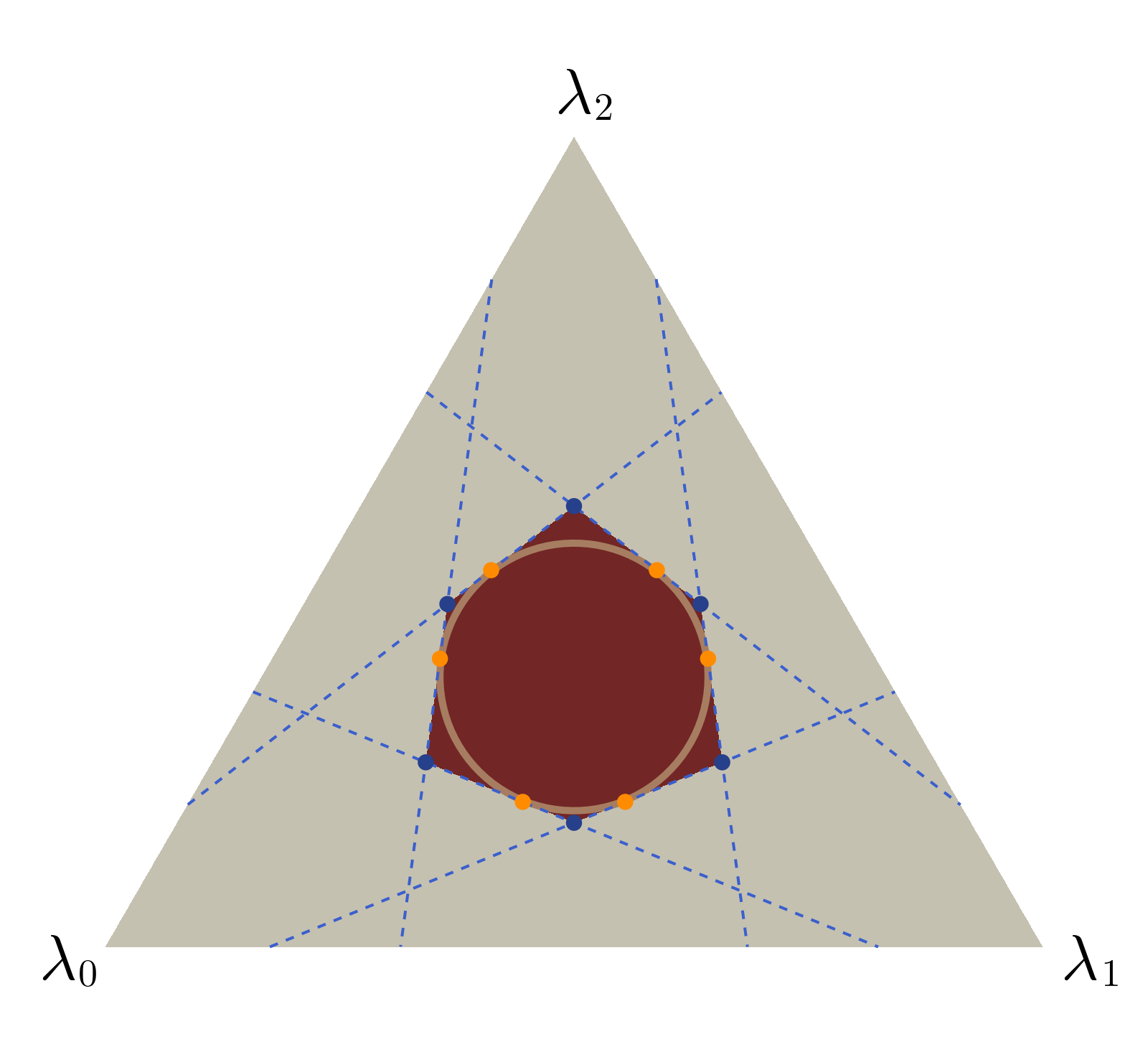
Figure 1: AWP polytope for $j=1$ displayed in the barycentric coordinate system. The AWP polytope is the area shaded in dark red with the blue dashed lines marking the hyperplanes defined by Eq. (24). The circle is the surface of the AWP ball (see Section 4). The orange points represent all the permutations of the spectrum (37). The gray triangle corresponds to the full simplex of spin-$1$ states with spectrum $\bm{\lambda}=(\lambda_{0},\lambda_{1},\lambda_{2})$.

These vertices can be found as follows. In general we need $2j+1$ independent conditions on the vector $(\lambda_{0},\lambda_{1},\ldots,\lambda_{2j})$ to uniquely define (the unitary orbit of) a state $\rho$. One of them is given by the normalization condition $\sum_{i=0}^{2j}\lambda_{i}=1$. The others correspond to the fact that a vertex of the AWP polytope is the intersection of $2j$ hyperplanes each specified by an equation of the form (24). One of them is

$$\sum_{i=0}^{2j}\lambda_{i}^{\downarrow}\Delta_{i}^{\uparrow}=0.$$ (25)

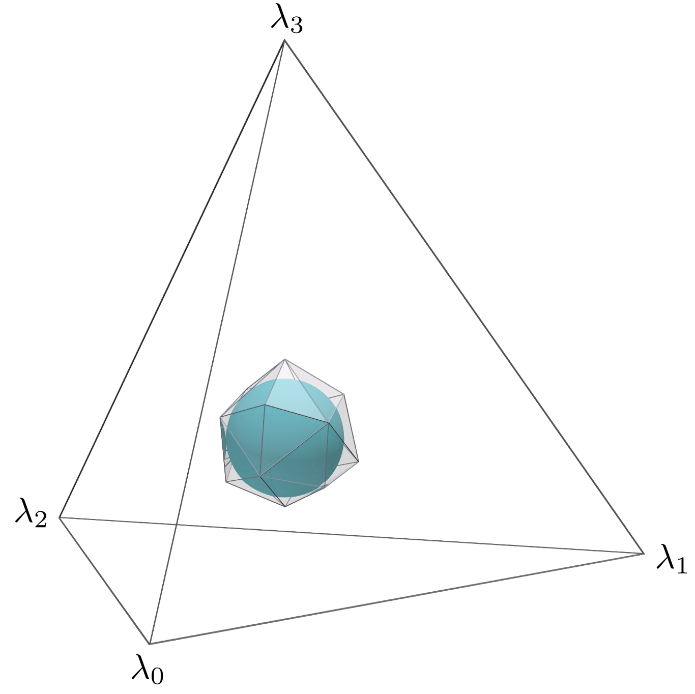
Figure 2: The AWP polytope for $j=3/2$ in the barycentric coordinate system (top). The grey rods (shown in the enlarged polytope at the bottom) are the edges of the AWP polytope and the blue sphere is its largest inner ball, with radius $r_{\mathrm{in}}^{\mathrm{AWP}}=1/(2\sqrt{15})$.

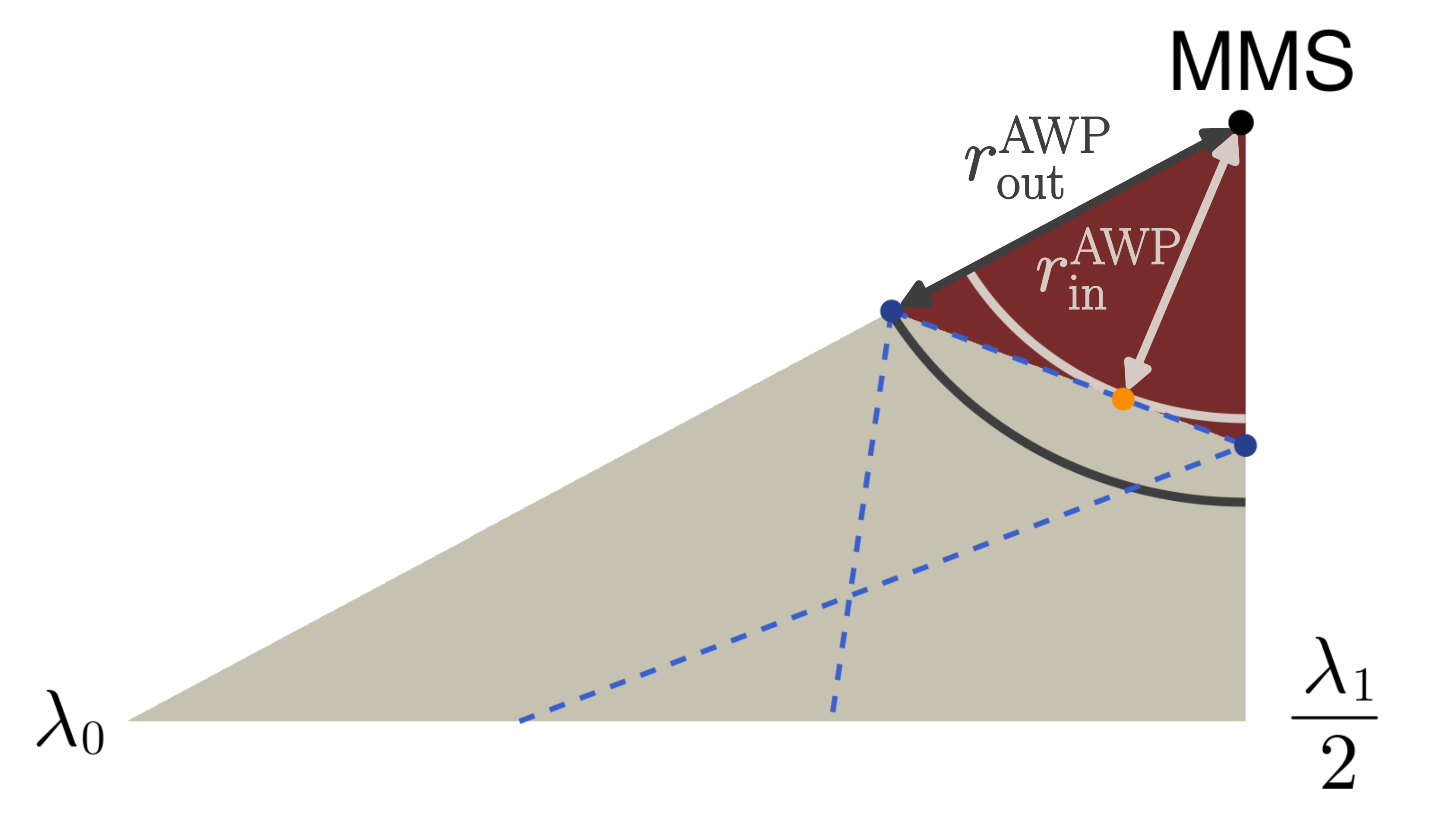
Figure 3: AWP minimal polytope for $j=1$ in the barycentric coordinate system. The structure is similar to Fig. 1 but we only draw the part where the eigenvalues of the state are ordered in descending value. The dark point corresponds to the maximally mixed state (MMS). The inner and outer AWP balls radii, $r_{\mathrm{in}}^{\mathrm{AWP}}$ and $r_{\mathrm{out}}^{\mathrm{AWP}}$, are shown.

Let us focus on the remaining $2j-1$. For simplicity, consider a transposition $\pi=(p,q)$ with $q>p$. The condition (24) becomes in this case, using (25),

$$\lambda_{p}^{\downarrow}\Delta_{q}^{\uparrow}+\lambda_{q}^{\downarrow}\Delta_{p}^{\uparrow}+\sum_{\begin{subarray}{c}i=0\\ i\neq p,q\end{subarray}}^{2j}\lambda_{i}^{\downarrow}\Delta_{i}^{\uparrow}=0$$

$$\Leftrightarrow\quad \lambda_{p}^{\downarrow}(\Delta_{q}^{\uparrow}-\Delta_{p}^{\uparrow})+\lambda_{q}^{\downarrow}(\Delta_{p}^{\uparrow}-\Delta_{q}^{\uparrow})=0$$ (26)

As all the eigenvalues of the kernel are different by assumption (12), Eq. (3.2) is satisfied iff $\lambda_{p}^{\downarrow}=\lambda_{q}^{\downarrow}$ and, as the eigenvalues are ordered, this also means that $\lambda_{k}^{\downarrow}=\lambda_{p}^{\downarrow}$ for all $k$ between $p$ and $q$. Note that in this reasoning, the only forbidden transposition is $(0,2j)$ because it would give the MMS. Hence, for a given transposition $(p,q)$ will correspond a set of $q-p$ conditions $\lambda_{l}=\lambda_{l+1}$ for $l=p,\ldots,q-1$. Therefore, as any permutation is a composition of transpositions, the $2j-1$ conditions that follow from (24) eventually reduce to a set of $2j-1$ nearest-neighbour eigenvalue equalities taken from

$$\mathcal{E}=\left(\lambda_{0}^{\downarrow}=\lambda_{1}^{\downarrow},\lambda_{1}^{\downarrow}=\lambda_{2}^{\downarrow},...,\lambda_{2j-1}^{\downarrow}=\lambda_{2j}^{\downarrow}\right).$$ (27)

Since we need $2j-1$ conditions, we can draw $2j-1$ equalities from $\mathcal{E}$ in order to obtain a vertex. This method gives $\binom{2j}{2j-1}=2j$ different draws and so we get $2j$ vertices for the minimal polytope. As explained previously, all other vertices of the full polytope are obtained by permuting the coordinates of the vertices of the minimal polytope. In Appendix C, we give the barycentric coordinates of the vertices of the minimal polytope up to $j=2$. The entirety of the preceding discussion of the AWP polytope vertices naturally extends to the AWB polytope vertices for which we must replace $0$ by $W_{\text{min}}$ in the right-hand side of the equality (24). However, for negative values of $W_{\text{min}}$, the polytope may be partially outside the simplex and some vertices will have negative-valued components, resulting in unphysical states.

A peculiar characteristic of the AWP polytope is that each point on its surface has a state in its orbit satisfying $W(0)=0$. Indeed, for an eigenspectrum $\bm{\lambda}$ that satisfies (24) for a given permutation $\pi$, the diagonal state $\rho$ in the Dicke basis with $\rho_{ii}=\lambda_{\pi^{-1}(i)}$ satisfies

$$W(0)=\sum_{i=0}^{2j}\lambda_{i}\Delta_{i}=0$$ (28)

and is in the unitary orbit of $\bm{\lambda}$. Following the same reasoning, in the interior of the AWP polytope, there is no state with a zero-valued Wigner function.

3.3 Majorization condition

Here we find a condition equivalent to (15) for a state to be AWB based on its majorization by a mixture of the vertices of the minimal polytope.

Definition 2.

For two vectors $\mathbf{u}$ and $\mathbf{v}$ of the same length $n$, we say that $\mathbf{u}$ majorizes $\mathbf{v}$, denoted $\mathbf{u}\succ\mathbf{v}$, iff

$$\sum_{k=1}^{l}u_{k}^{\downarrow}\geq\sum_{k=1}^{l}v_{k}^{\downarrow}$$ (29)

for $l<n$, with $\sum_{k=1}^{n}u_{k}=\sum_{k=1}^{n}v_{k}$ and $\mathbf{u}^{\downarrow}$ denoting the vector $\mathbf{u}$ with components sorted in decreasing order.

Proposition 2.

A state $\rho$ is AWB iff its eigenvalues $\bm{\lambda}$ are majorized by a convex combination of the ordered vertices $\{\bm{\lambda}^{\downarrow}_{\mathrm{v}_{k}}\}$ of the corresponding AWB polytope, i.e. $\exists\,\mathbf{c}\in\mathbb{R}_{+}^{2j}$ such that

$$\bm{\lambda}\prec\sum_{k=1}^{2j}c_{k}\bm{\lambda}^{\downarrow}_{\mathrm{v}_{k}}$$ (30)

with $\sum_{k=1}^{2j}c_{k}=1$.

Proof.

If $\bm{\lambda}$ is AWB then it can be expressed as a mixture of the vertices of the AWB polytope

$$\bm{\lambda}=\sum_{k}c_{k}\bm{\lambda}_{\text{v}_{k}}$$ (31)

and the majorization (30) follows.

Conversely, it is known from the Schur-Horn theorem that $\mathbf{x}\succ\mathbf{y}$ iff $\mathbf{y}$ is in the convex hull of the vectors obtained by permuting the elements of $\mathbf{x}$ (i.e. the permutahedron generated by $\mathbf{x}$). Hence, if $\bm{\lambda}$ respects (30), it can be expressed as a convex combination of the vertices of the AWB polytope and is therefore inside it. ∎

4 Balls of absolutely Wigner bounded states

4.1 Largest inner ball of the AWB polytope

In this section, we calculate the radius $r_{\mathrm{in}}^{W_{\mathrm{min}}}$ of the largest ball centred on the MMS contained in the polytope of AWB states and find a state $\rho^{*}$ that is both on the surface of this ball and on a face of the polytope. Denoting by $r(\rho)$ the Hilbert-Schmidt distance between a state $\rho$ and the MMS,

$$r(\rho)=\lVert\rho-\rho_{0}\rVert_{\mathrm{HS}}=\sqrt{\mathrm{Tr}\left[\left(\rho-\rho_{0}\right)^{2}\right]},$$ (32)

we have that all valid states with $r(\rho)\leq r_{\mathrm{in}}^{W_{\mathrm{min}}}$ are AWB.

Proposition 3.

The radius of the largest inner ball of the AWB polytope associated with a $W_{\mathrm{min}}$ value such that the ball is contained within the state simplex is

$$r_{\mathrm{in}}^{W_{\mathrm{min}}}=\frac{1-(2j+1)W_{\mathrm{min}}}{2\sqrt{j(2j+1)(j+1)}}.$$ (33)

Proof.

Note that the distance (32) is equivalent to the Euclidean distance in the simplex between the spectra $\bm{\lambda}$ and $\bm{\lambda}_{0}$ of $\rho$ and the MMS respectively, i.e.

$$r(\rho)=\sqrt{\left(\sum_{i=0}^{2j}\lambda_{i}^{2}\right)-\frac{1}{2j+1}}=\lVert\bm{\lambda}-\bm{\lambda}_{0}\rVert.$$

In order to find the radius $r_{\mathrm{in}}^{W_{\mathrm{min}}}$ (see Fig. 3 for $W_{\mathrm{min}}=0$) of the largest inner ball of the AWB polytope, we need to find the spectra on the hyperplanes of the AWB polytope with the minimum distance to the MMS. Mathematically, this translates in the following constrained minimization problem

$$\min_{\bm{\lambda}}\;\lVert\bm{\lambda}-\bm{\lambda}_{0}\rVert^{2}\;\;\;\text{ subject to }\left\{\begin{array}[]{l}\sum_{i=0}^{2j}\lambda_{i}=1\\[8.0pt] \bm{\lambda\cdot\Delta}=W_{\mathrm{min}}\end{array}\right.$$ (34)

where $\bm{\Delta}=\left(\Delta_{0},\Delta_{1},...,,\Delta_{2j}\right)$. For this purpose, we use the method of Lagrange multipliers with the Lagrangian

$$L=\lVert\bm{\lambda}-\bm{\lambda}_{0}\rVert^{2}+\mu_{1}\left(\bm{\lambda\cdot\Delta}-W_{\mathrm{min}}\right)+\mu_{2}\left(1-\sum_{i=0}^{2j}\lambda_{i}\right)$$

where $\mu_{1},\mu_{2}$ are two Lagrange multipliers to be determined. The stationary points $\bm{\lambda}^{*}$ of the Lagrangian must satisfy the following condition

$$\frac{\partial L}{\partial\bm{\lambda}}\Big{|}_{\bm{\lambda}=\bm{\lambda}^{*}}=\bm{0}\quad\Leftrightarrow\quad 2\bm{\lambda}^{*}+\mu_{1}\bm{\Delta}-\mu_{2}\bm{1}=\bm{0}$$ (35)

with $\bm{1}=(1,1,...,1)$ of length $2j+1$. By summing over the components of (35) and using Eq. (10), we readily get

$$\mu_{2}=\frac{\mu_{1}+2}{2j+1}.$$ (36)

Then, by taking the scalar product of (35) with $\bm{\Delta}$ and using Eqs. (11) and (36), we obtain

$$\mu_{1}=\frac{1-(2j+1)W_{\mathrm{min}}}{2j(j+1)}\quad\mathrm{and}\quad\mu_{2}=\frac{(2j+1)-W_{\mathrm{min}}}{2j(j+1)}.$$

Finally, by substituting the above values for $\mu_{1}$ and $\mu_{2}$ in Eq. (35) and solving for the stationary point $\bm{\lambda}^{*}$, we get

$$\bm{\lambda}^{*}=\frac{\left[(2j+1)-W_{\mathrm{min}}\right]\bm{1}-\left[1-(2j+1)W_{\mathrm{min}}\right]\bm{\Delta}}{4j(j+1)}$$ (37)

from which the inner ball radius follows as

$$r_{\mathrm{in}}^{W_{\mathrm{min}}}=r(\rho^{*})=\frac{1-(2j+1)W_{\mathrm{min}}}{2\sqrt{j(2j+1)(j+1)}}$$

with $\rho^{*}$ a state with eigenspectrum (37). ∎

Let us first consider positive values of $W_{\mathrm{min}}$. The inner radius (33) vanishes for $W_{\mathrm{min}}=1/(2j+1)$, corresponding to the fact that only the MMS state has a Wigner function with this minimal (and constant) value. The radius then increases as $W_{\mathrm{min}}$ decreases. At $W_{\mathrm{min}}=0$, it reduces to the radius of the largest ball of AWP states,

$$r_{\mathrm{in}}^{\mathrm{AWP}}=\frac{1}{2\sqrt{j(2j+1)(j+1)}}.$$ (38)

Expressed as a function of dimension $N=2j+1$ and re-scaled to generalized Bloch length, this result was also recently found in the context of SU($N$)-covariant Wigner functions (i.e. as the phase space manifold changes dramatically with each Hilbert space dimension, rather than always being the sphere) [26]. While our bound is tight for all $j$ in the SU(2) setting (i.e. there always exist orbits infinitesimally further away that contain Wigner-negative states), it is unknown if this bound remains tight for such SU($N$)-covariant Wigner functions for $N>2$.

At the critical value

$$W_{\mathrm{min}}=\frac{\Delta_{j,j}-(2j+1)}{\Delta_{j,j}(2j+1)-1}<0,$$ (39)

the spectrum (37) acquires a first zero eigenvalue, $\lambda^{*}_{2j}=0$. This corresponds to the situation where $\bm{\lambda}^{*}$ is simultaneously on the surface of the ball, on a face of the polytope and on an edge of the simplex as seen in Fig. 4. For more negative values of $W_{\mathrm{min}}$, Eq. (37) no longer represents a physical state because $\lambda^{*}_{2j}$ becomes negative. In this situation, in order to determine the radius of larger balls containing only AWB states, additional constraints must be imposed in the optimisation procedure reflecting the fact that some elements of the spectrum of $\rho$ are zero. Since the possible number of zero eigenvalues depends on $j$, we will not go further in this development. Nevertheless, in the end, when there is only one non-zero eigenvalue left (equal to 1, in which case the states are pure), the most negative $W_{\mathrm{min}}$ corresponds to the smallest kernel eigenvalue $\Delta_{j.j-1}$ (according to the conjecture (12)), and the radius is the distance $r=\sqrt{2j/(2j+1)}$ from pure states to the MMS.

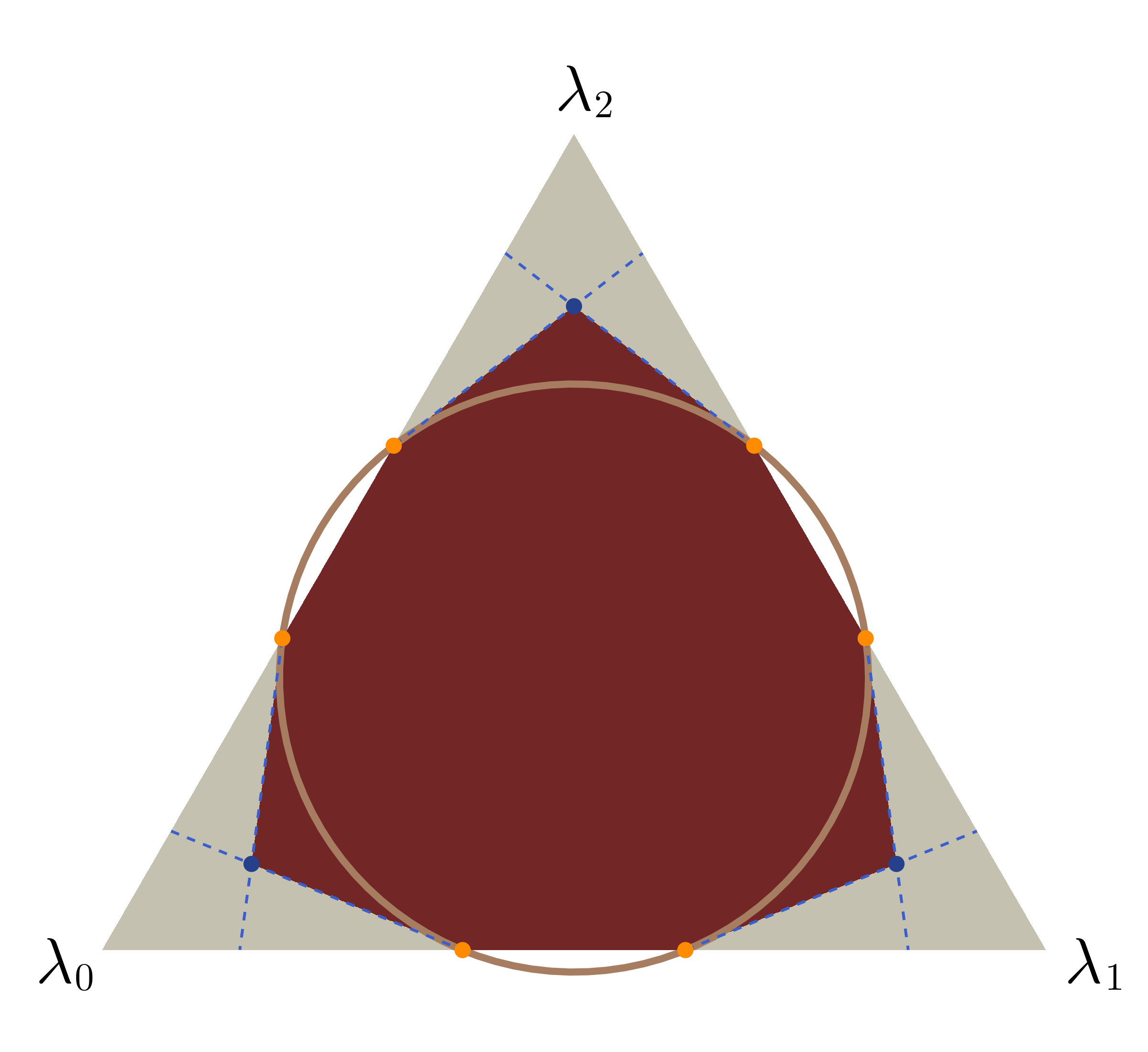
Figure 4: AWB polytope in the barycentric coordinate system for $j=1$ and $W_{\mathrm{min}}=\frac{1}{3}+\frac{2}{3}\sqrt{2}\left(\sqrt{5}-3\right)\approx-0.387$ as given by Eq. (39). The structure is similar to Fig. 1 but the polytope occupies a larger portion of the state space. We omit the part of the polytope that is outside the simplex.

Finally, it should be noted that any state resulting from the permutation of the elements of $\bm{\lambda}^{*}$ is also on the surface of the AWB inner ball and verify a similar equality as (24) for any permutation $\pi$. Thus by considering all permutations of the elements of $\bm{\lambda}^{*}$ we can find all states located where the AWB polytope is tangent to the AWB inner ball, as shown in Fig. 1 for $j=1$ and $W_{\mathrm{min}}=0$.

4.2 Smallest outer ball of the AWB polytope

We now formulate a conjecture for the radius $r_{\text{out}}^{W_{\mathrm{min}}}$ of the smallest outer ball of the polytope containing all AWB states. With the set of AWB states forming a convex polytope, $r_{\text{out}}^{W_{\mathrm{min}}}$ must be the radius associated with the outermost vertex. Hence the problem is equivalent to finding this furthest vertex of the minimal polytope. As mentioned above, as $W_{\mathrm{min}}$ gets smaller and the polytopes get bigger, both the polytopes and their the inner and outer Hilbert Schmidt balls will eventually encompass unphysical states. We therefore acknowledge that intermediate calculations may take us outside of the state simplex, but final results must of course be restricted to the intersection of these objects with the simplex. When a vertex lies inside the simplex it may be referred to as a vertex state.

In principle, this can always be determined on a case-by-case basis via the following procedure. Recall from Sec. 3.2 that an AWB state with ordered spectrum $\bm{\lambda}^{\downarrow}$ located on a vertex is specified by $2j+1$ linear eigenvalue constraints. The first is normalization, the second is the AWB vertex criterion (i.e. Eq. (25) with a $W_{\mathrm{min}}$), and the remaining $2j-1$ come from a ($2j-1$)-sized sample from the $(2j)$-sized set of nearest-neighbour constraints (27). Thus the $2j$ states sitting on the $2j$ distinct vertices match up with the $\binom{2j}{2j-1}=2j$ choices of bi-partitioning the ordered eigenvalues into a “left” set, $\bm{\omega}_{n}$, of size $n$ and a “right” set, $\bm{\sigma}_{n}$, of size $2j+1-n$, each of which contain eigenvalues of equal value $\omega_{n}$ and $\sigma_{n}$ respectively such that $\omega_{n}>\sigma_{n}$. The full eigenspectrum is the concatenation $\bm{\lambda}^{\downarrow}_{\mathrm{v}_{n}}=\bm{\omega}_{n}\circ\bm{\sigma}_{n}$, and normalization becomes

$$n\omega_{n}+(2j+1-n)\sigma_{n}=1,\quad n\in\{1,...,2j\}.$$ (40)

As we are temporarily allowing the ordered spectrum $\bm{\lambda}^{\downarrow}$ to have negative components, Eq. (40) should be interpreted only as requiring the vertices to lie in the hyperplane generated by the state simplex (i.e. not necessarily within the simplex). Inserting $\bm{\lambda}^{\downarrow}_{\mathrm{v}_{n}}$ and (40) into the AWB vertex criterion the weights $\omega_{n}$ can be solved as a function of the kernel eigenvalues and $W_{\mathrm{min}}$:

$$\omega_{n} =\frac{\sum_{i=n}^{2j}\Delta_{i}^{\uparrow}-(2j+1-n)W_{\mathrm{min}}}{n\sum_{i=n}^{2j}\Delta_{i}^{\uparrow}-(2j+1-n)\sum_{i=0}^{n-1}\Delta_{i}^{\uparrow}}$$

$$=\frac{\tau_{n}-(2j+1-n)W_{\mathrm{min}}}{(2j+1)\tau_{n}-(2j+1-n)}$$ (41)

where in the second line we used the unit-trace property (10) of the kernel and

$$\tau_{n}=\sum_{i=n}^{2j}\Delta_{i}^{\uparrow}=\sum_{i=0}^{2j-n}\Delta_{i}^{\downarrow}$$ (42)

is the sum over the largest $2j+1-n$ kernel eigenvalues. The purity $\gamma_{\mathrm{v}_{n}}$ and distance $r_{\mathrm{v}_{n}}$ of the $n$-th vertex is then given by

$$\gamma_{\mathrm{v}_{n}} =n\omega_{n}^{2}+(2j+1-n)\sigma_{n}^{2}$$ (43)

$$r_{\mathrm{v}_{n}} =\sqrt{\gamma_{\mathrm{v}_{n}}-\frac{1}{2j+1}},$$ (44)

which are functions of only the kernel eigenvalues and $W_{\mathrm{min}}$. Note that purity, being defined as the sum of squares of the eigenvalues, remains a faithful notion of distance to the MMS even when such spectra are allowed to go negative. After computing each of these numbers, $r_{\text{out}}^{W_{\mathrm{min}}}$ would correspond to the largest one, and the set of states satisfying this condition would be the intersection of the associated ball with the state simplex. In Sec. 5.2 we present details of this procedure for $j=1$ and $W_{\mathrm{min}}=0$.

Despite this somewhat involved procedure, we numerically find it is always the case that the first vertex, $\mathrm{v}_{1}$, remains within the state simplex for all $W_{\mathrm{min}}\in[\Delta^{\uparrow}_{0},\frac{1}{2j+1}]$ and, relatedly, that

$$r^{W_{\mathrm{min}}}_{\text{out}}=r_{\text{v}_{1}}.$$ (45)

We conjecture this to be true in all finite dimensions. Part of the difficulty in proving this in general comes from the non-trivial nature of the kernel eigenvalues (8) and from further numerical evidence suggesting that no vertex state ever majorizes any other vertex state.

Furthermore, with the most negative kernel eigenvalue (12) being $\Delta^{\uparrow}_{0}=\Delta_{j,j-1}$, the vertex state $\rho_{\text{v}_{1}}$ takes the special form

$$\omega_{1}{\left|{j,j-1}\right\rangle\!\!\left\langle{j,j-1}\right|}+\frac{1-\omega_{1}}{2j}\sum_{m\neq j-1}{\left|{j,m}\right\rangle\!\!\left\langle{j,m}\right|}$$ (46)

where

$$\omega_{1} =\frac{\sum_{m\neq j-1}\Delta_{j,m}-2jW_{\mathrm{min}}}{\sum_{m\neq j-1}\Delta_{j,m}-2j\Delta_{j,j-1}}$$

$$=\frac{1-\Delta_{j,j-1}-2jW_{\mathrm{min}}}{1-(2j+1)\Delta_{j,j-1}}.$$ (47)

The minimal outer radius $r_{\text{out}}^{W_{\mathrm{min}}}$ is then conjectured to be

$$r_{\text{out}}^{W_{\mathrm{min}}} =\sqrt{\gamma_{\text{v}_{1}}-\frac{1}{2j+1}}$$

$$=\sqrt{\omega_{1}^{2}+2j\left(\frac{1-\omega_{1}}{2j}\right)^{2}-\frac{1}{2j+1}}.$$ (48)

An operational interpretation of this radius is available by noting that the multiqubit realization of the ${|{j,j-1}\rangle}$ state, which has the most pointwise-negative Wigner function allowable (occurring at the North pole), is in fact the $W$ state introduced in the context of LOCC entanglement classification [40]. And since the maximally mixed state has uniform eigenvalues, Eq. (46) may be interpreted as the end result of mixing the $W$ state with the maximally mixed state until the Wigner function at the North pole hits $W_{\mathrm{min}}$. The distance between the resulting state and the maximally mixed state is exactly our conjectured $r_{\text{out}}^{W_{\mathrm{min}}}$. In particular, when the Wigner function vanishes at the North pole, the radius reduces to a tight, purity-based AWP necessity condition.

Finally, when the lower bound is set to $W_{\mathrm{min}}=\Delta_{j,j-1}$, Eq. (47) becomes unity and the outer radius becomes the Hilbert-Schmidt distance to pure states, which reflects the fact that now the entire simplex is contained within the AWB polytope.

5 Relationship with entanglement and absolute Glauber-Sudarshan positivity

Another common quasi-probability distribution studied in the context of single spins is the Glauber-Sudarshan $P$ function, defined through the equality

$$\rho=\frac{2j+1}{4\pi}\int P_{\rho}(\Omega)\,{|{\Omega}\rangle}{\left\langle{\Omega}\right|}\,d\Omega,$$ (49)

Compared to the Wigner function, the $P$ function is not unique. Negative values of all $P$ functions representing the same state can be interpreted as the presence of entanglement within the multi-qubit realization of the system [29]. In other words, a general state $\rho$ of a single spin-$j$ system admits a positive $P$ function if and only if the many-body realization is separable (necessarily over symmetric states). This follows from the definition (49) of the $P$ function as the expansion coefficients of a state $\rho$ in the spin coherent state projector basis, and the fact that spin coherent states are the only pure product states available when the qubits are indistinguishable.

States that admit a positive $P$ function after any global unitary transformation are called absolutely classical spin states [30] or symmetric absolutely separable (SAS) states [22]. In this section we focus entirely on the case of $W_{\mathrm{min}}=0$ because negative values of the Wigner function are generally used as a witness of non-classicality and compare the AWP polytopes to the known results on SAS states. In the context of single spins, the set of SAS states is only completely characterized for spin-1/2 and spin-1. We also show that the Wigner negativity (6) of a positive-valued $P$-function state is upper-bounded by the Wigner negativity of a coherent state.

5.1 Spin-1/2

In the familiar case of a single qubit state $\rho$, the spectrum $(\lambda,1-\lambda)$ is characterized by one number $\lambda$. The kernel eigenvalues, Eq. (8), are

$$\Delta_{0}=\frac{1}{2}(1-\sqrt{3}),\quad\Delta_{1}=\frac{1}{2}(1+\sqrt{3})=1-\Delta_{0}.$$ (50)

Letting $\lambda\geq\frac{1}{2}$ denote the larger of the two eigenvalues, the strong ordered form (22) becomes

$$\begin{split}\lambda_{0}\Delta_{0}+\lambda_{1}\Delta_{1}&=\lambda\Delta_{0}+(1-\lambda)(1-\Delta_{0})\\ &=\lambda(2\Delta_{0}-1)+1-\Delta_{0}.\end{split}$$ (51)

Thus the AWP polytope is described, in the 1-dimensional projection to the $\lambda$ axis, as

$$\frac{1}{2}\leq\lambda\leq\frac{1-\Delta_{0}}{1-2\Delta_{0}}=\frac{1}{2}+\frac{1}{2\sqrt{3}}.$$ (52)

This may be equivalently expressed either in terms of purity $\gamma$ or Bloch length $|\mathbf{n}|=\sqrt{2\gamma-1}$,

$$\frac{1}{2}\leq\gamma\leq\frac{2}{3}\qquad\text{and}\qquad|\mathbf{n}|\leq\frac{1}{\sqrt{3}}.$$ (53)

Additionally, the distance to the maximally mixed state via Eq. (32) is $r\leq 1/\sqrt{6}$, which matches with the smallest ball of AWP states derived earlier, Eq. (33). In the case of spin-1/2 this radius coincides with the largest ball containing nothing but AWP states.

Regarding absolute $P$-positivity, all qubit states are SAS. This is a consequence of the Bloch ball being the convex hull of the spin-$\frac{1}{2}$ coherent states and global unitaries corresponding only to rigid rotations. Thus AWP qubit states are a strict subset of SAS qubit states.

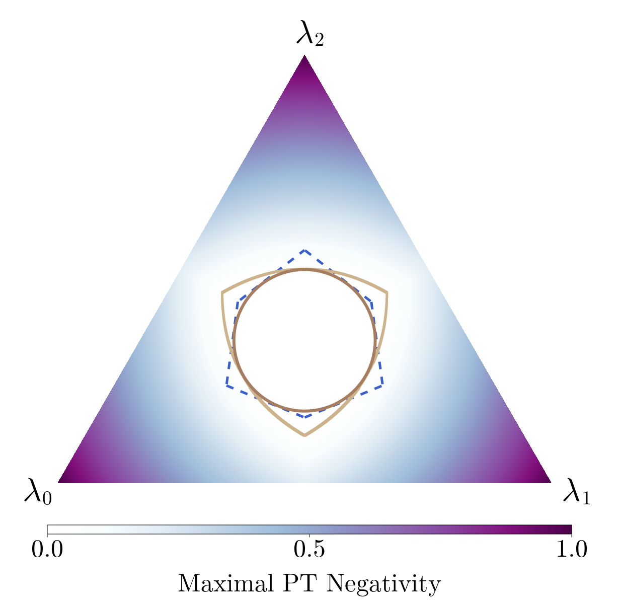
Figure 5: Maximal PT negativity over each unitary orbit in the $j=1$ simplex of state spectra. The dashed blue line and red circle are respectively the AWP polytope and ball. The camel curve shows the boundary at which the negativity along the unitary orbit becomes non-zero.

Furthermore, due to the invariance of negativity under rigid rotation, for a single qubit there is no distinction between a state being positive (in either the Wigner or $P$ sense) and being absolutely positive. This means that any state with Bloch radius $|\mathbf{n}|\in(1/\sqrt{3},1]$ has a positive $P$ function but a negative Wigner function. This is perhaps the simplest example of the fact that, unlike the planar phase space associated with optical systems, in spin systems Glauber-Sudarshan positivity does not imply Wigner positivity.

5.2 Spin-1

For qutrits the set of AWP states and the set of SAS states are both more complicated, with neither being a strict subset of the other. For SAS states we need the following result in [22]: the maximal value of the negativity, in the sense of the PPT criterion, in the unitary orbit of a two-qubit symmetric (or equivalently a spin-1) state $\rho$ with spectrum $\lambda_{0}\geq\lambda_{1}\geq\lambda_{2}$ is

$$\max\left[0,\sqrt{\lambda_{0}^{2}+(\lambda_{1}-\lambda_{2})^{2}}-\lambda_{1}-\lambda_{2}\right].$$ (54)

In Fig. 5, we plot the resulting maximal negativity in the $j=1$ simplex with the AWP polytope. There are clearly regions of spectra that satisfy either, both, or neither of the AWP and SAS conditions. Thus already for spin-1 there exist states with a positive $P$ function and a negative $W$ function and vice-versa. For $j=1$ specifically, it was also shown in [22] that the largest ball of SAS states has a radius $r_{\mathrm{in}}^{P}=1/(2\sqrt{6})\approx 0.20412$, which is the same value as the radius $r_{\mathrm{in}}^{\mathrm{AWP}}=1/(2\sqrt{6})$. Hence, for $j=1$, the largest ball of AWP states coincides with the largest ball of SAS states as we can see in Fig. 5.

We now illustrate the procedure described in Sec. 4.2 and compute the vertex states and their radii for the case of spin-$1$. The two diagonal states associated to the vertices of the minimal polytope for $j=1$ (see Fig. 3) are

$$\rho_{\text{v}_{1}} =\omega_{1}{\left|{1,-1}\right\rangle\!\!\left\langle{1,-1}\right|}$$

$$\quad+\frac{1-\omega_{1}}{2}({\left|{1,0}\right\rangle\!\!\left\langle{1,0}\right|}+{\left|{1,1}\right\rangle\!\!\left\langle{1,1}\right|}),$$ (55)

$$\rho_{\text{v}_{2}} =\omega_{2}({\left|{1,-1}\right\rangle\!\!\left\langle{1,-1}\right|}+{\left|{1,0}\right\rangle\!\!\left\langle{1,0}\right|})$$

$$\quad+(1-2\omega_{2}){\left|{1,1}\right\rangle\!\!\left\langle{1,1}\right|}$$ (56)

where the parameters $\omega_{1}$ and $\omega_{2}$ are found by solving the AWP criterion (25):

$$\begin{split}\omega_{1}&=\frac{\Delta_{1,-1}+\Delta_{1,1}}{\Delta_{1,-1}+\Delta_{1,1}-2\Delta_{1,0}}=\frac{1}{15}(5+\sqrt{10}),\\ \omega_{2}&=\frac{\Delta_{1,1}}{2\Delta_{1,1}-\Delta_{1,0}-\Delta_{1,-1}}=\frac{1}{6}\left(2+\sqrt{7-3\sqrt{5}}\right).\end{split}$$ (57)

The two Hilbert-Schmidt radii (32) of the vertex states are then

$$\begin{split}r_{\text{v}_{1}}&=r_{\text{out}}^{\mathrm{AWP}}=\frac{1}{\sqrt{15}}\approx 0.2582,\\ r_{\text{v}_{2}}&=\sqrt{\frac{1}{6}\left(7-3\sqrt{5}\right)}\approx 0.2205.\end{split}$$ (58)

As conjectured, we see that $r_{\text{v}_{1}}=r_{\text{out}}^{W}$ for spin-1.

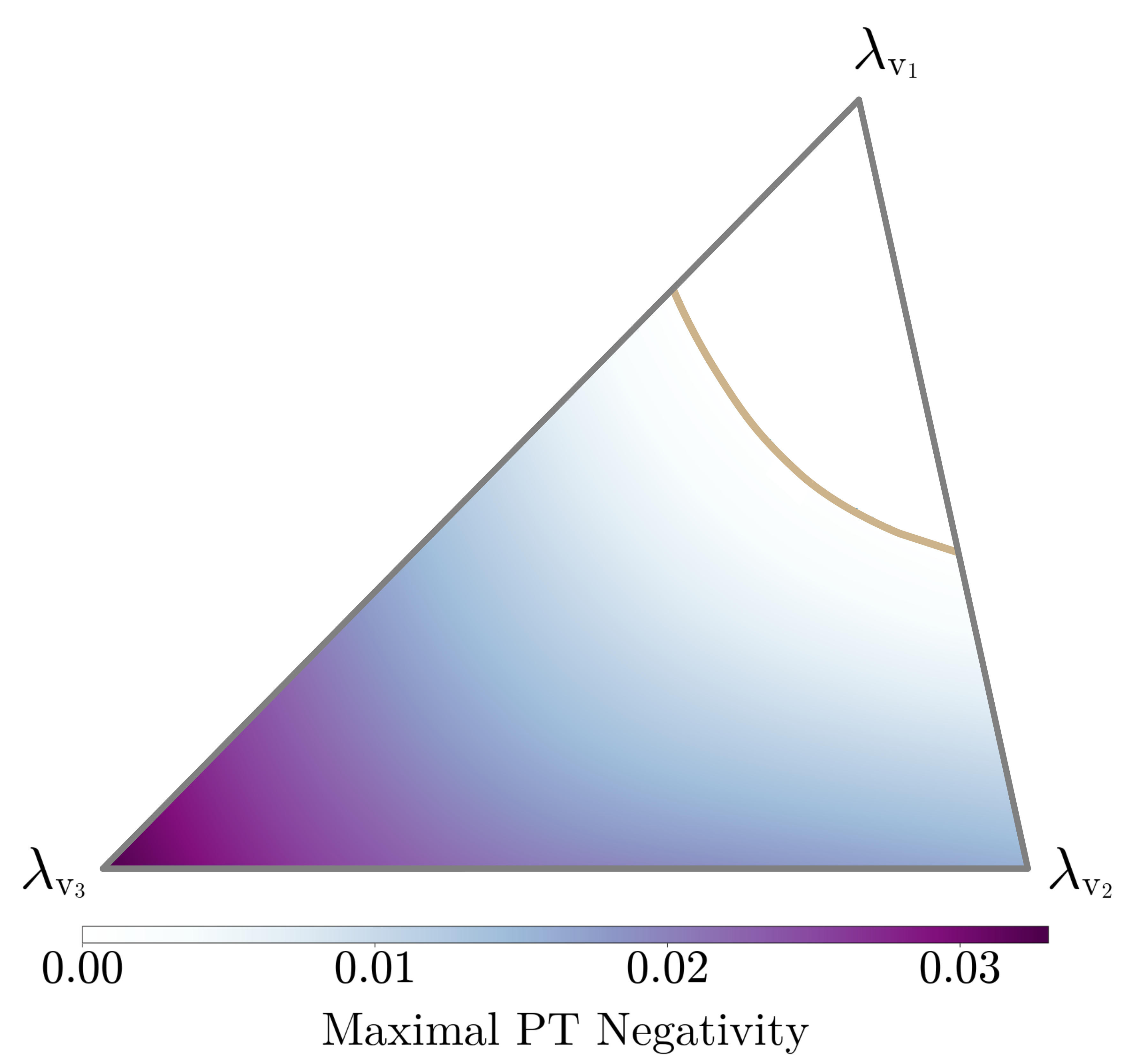
Figure 6: Maximal PT negativity over each unitary orbit on the face of the minimal $j=3/2$ AWP polytope. The camel curve shows the boundary at which the negativity along the unitary orbit becomes non-zero. The notation of the vertices corresponds to the eigenspectra given in Table 1.

5.3 Spin-3/2

For spin-$3/2$, a numerical optimization (see Ref. [22] for more information) yielded the maximum negativity (in the sense of the negativity of the partial transpose of the state) in the unitary orbit of the states located on a face of the polytope. The results are displayed in Fig. 6 where, similar to the spin-1 case, we observe both SAS and entangled states on the face of the minimal AWP polytope. A notable difference is that, for $j=3/2$, the largest ball containing only SAS states has a radius $r_{\mathrm{in}}^{P}=1/(2\sqrt{19})$ [22] which is strictly smaller than $r_{\mathrm{in}}^{\mathrm{AWP}}=1/(2\sqrt{15})$. Therefore, the SAS states on the face of the polytope are necessarily outside this ball.

5.4 Spin-$j>3/2$

In Fig. 7, we compare the radius of the AWP ball (33) with the lower bound on the radius of the ball of SAS states [30]

$$r^{P}\equiv\frac{\left[(4j+1)\tbinom{4j}{2j}-(j+1)\right]^{-1/2}}{\sqrt{4j+2}}\leq r^{P}_{\mathrm{in}}.$$ (59)

This plot suggests that the balls of AWP states can be much larger than the balls of SAS states. This is confirmed by our numerical observations that sampling the hypersurface of the polytope for $j=2$, $5/2$ and $3$ always yields states that have negative partial transpose in their unitary orbit. We also plot in Fig. 7 the conjectured radius $r_{\mathrm{out}}^{\mathrm{AWP}}$ of the minimal ball containing all AWP states. Notably, the scalings of $r_{\mathrm{out}}^{\mathrm{AWP}}$ and $r_{\mathrm{in}}^{\mathrm{AWP}}$ with $j$ are different. The scaling $r_{\mathrm{in}}^{\mathrm{AWP}}\propto j^{-3/2}$ follows directly from Eq. (33). The scaling $r_{\mathrm{out}}^{\mathrm{AWP}}\propto j^{-1}$ can be explained by noting that the infinite-spin limit of the SU(2) Wigner kernel is the Heisenberg-Weyl Wigner kernel, which only has the two eigenvalues $\pm 2$ [27]. Hence for sufficiently large $j$ we may approximate $\Delta_{j,j-1}\approx-2$, which yields $\omega_{1}\approx 3/(3+4j)$ from (47). The Laurent series of Eq. (48) with this approximation has leading term $1/(4j)$, exactly matching the results shown in Fig. 7.

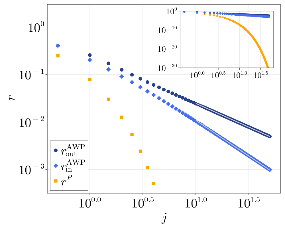
Figure 7: Comparison of the radii of the outer AWP ball (dark blue) and the inner AWP ball (blue) and the lower bound on the SAS ball radius (orange). For $j\geq 10$, we found excellent fits with $r_{\mathrm{out,fit}}^{\mathrm{AWP}}=0.25\times j^{-1}$ and $r_{\mathrm{in,fit}}^{\mathrm{AWP}}=0.336\times j^{-1.5}$. These are explained in the text.

5.5 Bound on Wigner negativity

The spin-1 case showed us that there are SAS states outside the AWP polytope, i.e. with a Wigner function admitting negative values. Here, we show very generally that the Wigner negativity (6) of states with an everywhere positive $P$ function (in particular SAS states), denoted hereafter by $\rho_{P\geqslant 0}$, is upper bounded by the Wigner negativity of coherent states. Indeed, such states can always be represented as a mixture of coherent states

$$\rho_{P\geqslant 0}=\sum_{i}w_{i}\left|\alpha_{i}\right\rangle\left\langle\alpha_{i}\right|$$ (60)

with $w_{i}\geqslant 0$ and $\sum_{i}w_{i}=1$. Their Wigner negativity can then be upper bounded as follows

$$\delta(\rho_{P\geqslant 0}) =\frac{1}{2}\int_{\Gamma}\left|W_{\rho_{P\geqslant 0}}(\Omega)\right|d\mu(\Omega)-\frac{1}{2}$$ (61)

$$=\frac{1}{2}\int_{\Gamma}\left|\sum_{i}w_{i}W_{\left|\alpha_{i}\right\rangle}(\Omega)\right|d\mu(\Omega)-\frac{1}{2}$$

$$\leqslant\underbrace{\sum_{i}w_{i}}_{=1}\underbrace{\left(\frac{1}{2}\int_{\Gamma}\left|W_{\left|\alpha_{i}\right\rangle}(\Omega)\right|d\mu(\Omega)\right)}_{=\delta\left(|\alpha\rangle\right)+\frac{1}{2}}-\frac{1}{2}$$

$$=\delta\left(|\alpha\rangle\right)$$

where $\delta\left(|\alpha\rangle\right)$ is the Wigner negativity of a coherent state. Since it has been observed that the negativity of a coherent state decreases with $j$ [37], the same is true for positive $P$ function states.

6 Conclusion

We have investigated the non-classicality of unitary orbits of mixed spin-$j$ states. Our first result is Proposition 1, which gives a complete characterization for any spin quantum number $j$ of the set of absolutely Wigner bounded (AWB) states in the form of a polytope centred on the maximally mixed state in the simplex of mixed spin states. This amounts to an extension and alternative derivation of results from [25, 24] in the setting of quantum spin. We have studied the properties of the vertices of this polytope for different spin quantum numbers, as well as of its largest/smallest inner/outer Hilbert-Schmidt balls. In particular, we have shown that the radii of the inner and outer balls scale differently as a function of $j$ (see Eqs. (33) and (48) as well as Fig. 7). We have provided an equivalent condition for a state to be AWB based on majorization theory (Proposition 2). We have also compared our results on the positivity of the Wigner function with those on the positivity of the spherical Glauber-Sudarshan function, which can be equivalently used as a classicality criterion for spin states or a separability criterion for symmetric multiqubit states. The spin-1 and spin-3/2 cases, for which analytical results are known, were closely examined and important differences were highlighted, such as the existence of Wigner-negative absolutely separable states, and, conversely, the existence of entangled absolutely Wigner-positive states. However, a notable observation drawn from our numerics is that the set of SAS states appears to shrink relative to the set of AWP states as $j$ increases, which in turn occupies a progressively smaller volume of the simplex. Further research is needed to explore this behaviour. A related direction for future work could be to explore the ratio of the volume of the AWB polytopes to the volume of the full simplex; this would basically be a global indicator of classicality like those introduced and studied in Refs. [23, 25, 26] particularised to spin systems.

Another perspective, as briefly mentioned in Sec. 3, is to apply the techniques presented here to other distinguished quasiprobability distributions. For example, preliminary results suggest that the absolutely Husimi bounded (AHB) polytopes have the same geometry as the simplex, but are simply reduced in size by a factor depending on $Q_{\mathrm{min}}\in[0,\tfrac{1}{2j+1}]$. Future work could explore this further and investigate its consequences for the geometric measure of entanglement of multiqubit symmetric states. Another idea is to study how these polytopes change with respect to the spherical $s$-ordering parameter (see Eq. (23)).

Finally, given the importance of Wigner negativity in fields like quantum information science, our results shed new and interesting light on its manifestation in spin-$j$ systems, focusing on its relation to purity and entanglement. We believe that this will be relevant for various quantum information processing tasks, in particular those involving the symmetric subspace.

Appendix A Proof of relation (11)

We show here that the eigenvalues $\Delta_{m}\equiv\Delta_{j,m}$ of the Wigner kernel (1) verify

$$\sum_{m=-j}^{j}\Delta_{m}^{2}=2j+1.$$ (62)

Using the expression (8) we get

$$\sum_{m=-j}^{j}\Delta_{m}^{2}=\sum_{m=-j}^{j}\sum_{L,L^{\prime}=0}^{2j} \frac{(2L+1)(2L^{\prime}+1)}{(2j+1)^{2}}$$ (63)

$$\times C_{j,m;L,0}^{j,m}C_{j,m;L^{\prime},0}^{j,m}$$

The Clebsh-Gordan coefficients satisfy the following relations [34]

$$C_{a,\alpha;b,\beta}^{c,\gamma}=(-1)^{a-\alpha}\sqrt{\frac{2c+1}{2b+1}}C_{a,\alpha;c,-\gamma}^{b,-\beta}$$ (64)

$$\sum_{\alpha,\beta=-j}^{j}C_{a,\alpha;b,\beta}^{c,\gamma}C_{a,\alpha;b,\beta}^{c^{\prime},\gamma^{\prime}}=\delta_{cc^{\prime}}\delta_{\gamma\gamma^{\prime}}.$$ (65)

Hence, by splitting the sum over $m$ in two

$$\sum_{m}C_{j,m;L,0}^{j,m}C_{j,m;L^{\prime},0}^{j,m}=\sum_{m_{1},m_{2}}C_{j,m_{1};L,0}^{j,m_{2}}C_{j,m_{1};L^{\prime},0}^{j,m_{2}}$$ (66)

and using (64) and (65), we get from (63)

$$\sum_{m=-j}^{j}\Delta_{m}^{2} =\frac{1}{2j+1}\underbrace{\sum_{L=0}^{2j}2L+1}_{=(2j+1)^{2}}$$ (67)

$$=2j+1$$

Appendix B Barycentric coordinates

A mixed spin-$j$ state necessarily has eigenvalues $\lambda_{i}$ that are positive and add up to one:

$$\lambda_{i}\geq 0,\qquad\sum_{i=0}^{2j}\lambda_{i}=1.$$ (68)

This means that every state $\rho$ has its eigenvalue spectrum in the probability simplex of dimension $2j$. For example, for $j=1$, this simplex is a triangle shown in grey in Fig. 8. In geometric terms, the spectrum $(\lambda_{0},\lambda_{1},\lambda_{2})$ defines the barycentric coordinates of a point $\bm{\lambda}$ in the simplex, as it can be considered as the centre of mass of a system of $2j$ masses placed on the vertices of the triangle.

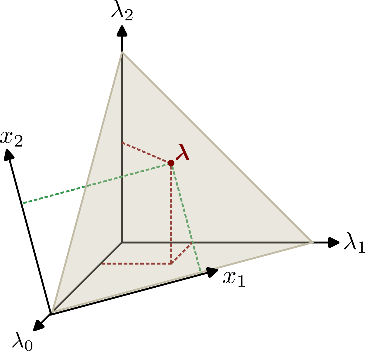
Figure 8: Barycentric and cartesian coordinate systems of spin state spectra for $j=1$. The simplex in this case is an equilateral triangle, shown here in gray. The red dot corresponds to a given spectrum and its projections onto the barycentric and Cartesian coordinate system are indicated by the red and green dashed lines respectively.

Let’s explain how to go from the barycentric coordinate system to the Cartesian coordinate system spanning the simplex. If we denote by $\{\mathbf{r}^{(i)}:i=0,\ldots,2j\}$ the set of $2j+1$ vertices of the simplex, the Cartesian coordinates of a point $\bm{\lambda}$ are given by

$$x_{k}=\sum_{i=0}^{2j}\lambda_{i}\,r_{k}^{(i)}$$ (69)

where $r_{k}^{(i)}$ is the $k$-th Cartesian coordinate of the $i$-th vertex of the simplex. For $j=1$, the simplex is an equilateral triangle with vertices having Cartesian coordinates $\mathbf{r}_{1}=(0,0)$, $\mathbf{r}_{2}=(1,0)$ and $\mathbf{r}_{3}=(1/2,\sqrt{3}/2)$. For $j=3/2$, it is a regular tetrahedron with vertices having Cartesian coordinates $\mathbf{r}_{1}=(0,0,0)$, $\mathbf{r}_{2}=(1,0,0)$, $\mathbf{r}_{3}=(1/2,\sqrt{3}/2,0)$ and $\mathbf{r}_{4}=(1/2,(2\sqrt{3})^{-1},\sqrt{2/3})$.

Appendix C AWP polytope vertices for $j\leq 2$

We give in Table 1 for $j\leq 2$ the spin state spectra associated with the vertices of the minimal AWP polytope as they can be determined as explained in Sec. 3.2.

$j$	Vertices in barycentric coordinates
1/2	$\bm{\lambda}_{\mathrm{v}_{1}}\approx$ (0.789, 0.211)
1	$\bm{\lambda}_{\mathrm{v}_{1}}\approx$ (0.423, 0.423, 0.153)
	$\bm{\lambda}_{\mathrm{v}_{2}}\approx$ (0.544, 0.228, 0.228)
3/2	$\bm{\lambda}_{\mathrm{v}_{1}}\approx$ (0.294, 0.294, 0.294, 0.119)
	$\bm{\lambda}_{\mathrm{v}_{2}}\approx$ (0.33, 0.33, 0.170, 0.170)
	$\bm{\lambda}_{\mathrm{v}_{3}}\approx$ (0.4, 0.2, 0.2, 0.2)
2	$\bm{\lambda}_{\mathrm{v}_{1}}\approx$ (0.313, 0.172, 0.172, 0.172, 0.172)
	$\bm{\lambda}_{\mathrm{v}_{2}}\approx$ (0.266, 0.266, 0.156, 0.156, 0.156)
	$\bm{\lambda}_{\mathrm{v}_{3}}\approx$ (0.24, 0.24, 0.24, 0.14, 0.14)
	$\bm{\lambda}_{\mathrm{v}_{4}}\approx$ (0.226, 0.226, 0.226, 0.226, 0.097)

Table 1: Barycentric coordinates (corresponding to the eigenspectrum of a mixed spin state) of the vertices of the minimal polytope of AWP states.

References

- [1] V. Veitch, C. Ferrie, D. Gross, and J. Emerson. “Negative quasi-probability as a resource for quantum computation”. New Journal of Physics 14, 113011 (2012).
- [2] A. Mari and J. Eisert. “Positive Wigner Functions Render Classical Simulation of Quantum Computation Efficient”. Phys. Rev. Lett. 109, 230503 (2012).
- [3] M. Howard, J. Wallman, V. Veitch, and J. Emerson. “Contextuality supplies the ‘magic’ for quantum computation”. Nature 510, 351–355 (2014).
- [4] N. Delfosse, C. Okay, J. Bermejo-Vega, D. E. Browne, and R. Raussendorf. “Equivalence between contextuality and negativity of the Wigner function for qudits”. New Journal of Physics 19, 123024 (2017).
- [5] R. I. Booth, U. Chabaud, and P.-E. Emeriau. “Contextuality and Wigner Negativity Are Equivalent for Continuous-Variable Quantum Measurements”. Phys. Rev. Lett. 129, 230401 (2022).
- [6] V. Veitch, S. A. Hamed Mousavian, D. Gottesman, and J. Emerson. “The resource theory of stabilizer quantum computation”. New Journal of Physics 16, 013009 (2014).
- [7] F. Albarelli, M. G. Genoni, M. G. A. Paris, and A. Ferraro. “Resource theory of quantum non-Gaussianity and Wigner negativity”. Phys. Rev. A 98, 052350 (2018).
- [8] X. Wang, M. M. Wilde, and Y. Su. “Quantifying the magic of quantum channels”. New Journal of Physics 21, 103002 (2019).
- [9] R. L. Hudson. “When is the Wigner quasi-probability density non-negative?”. Reports on Mathematical Physics 6, 249–252 (1974).
- [10] D. Gross. “Hudson’s theorem for finite-dimensional quantum systems”. Journal of Mathematical Physics 47, 122107 (2006).
- [11] J. M. Gracia-Bondá and J. C. Várilly. “Non-negative mixed states in Weyl-Wigner-Moyal theory”. Physics Letters A 128, 20–24 (1988).
- [12] T. Bröcker and R. F. Werner. “Mixed states with positive Wigner functions”. Journal of Mathematical Physics 36, 62–75 (1995).
- [13] A. Mandilara, E. Karpov, and N. J. Cerf. “Gaussianity bounds for quantum mixed states with a positive Wigner function”. Journal of Physics: Conference Series 254, 012011 (2010).
- [14] R. L. Stratonovich. “On Distributions in Representation Space”. Journal of Experimental and Theoretical Physics 4, 1012–1020 (1956). url: http://jetp.ras.ru/cgi-bin/e/index/e/4/6/p891?a=list.
- [15] J. C. Várilly and J. M. Gracia-Bondá. “The Moyal representation for spin”. Annals of Physics 190, 107–148 (1989).
- [16] J. P. Dowling, G. S. Agarwal, and W. P. Schleich. “Wigner distribution of a general angular-momentum state: Applications to a collection of two-level atoms”. Phys. Rev. A 49, 4101–4109 (1994).
- [17] A. B. Klimov, J. L. Romero, and H. de Guise. “Generalized SU(2) covariant Wigner functions and some of their applications”. Journal of Physics A: Mathematical and Theoretical 50, 323001 (2017).
- [18] B. Koczor, R. Zeier, and S. J. Glaser. “Continuous phase-space representations for finite-dimensional quantum states and their tomography”. Phys. Rev. A 101, 022318 (2020).
- [19] A. W. Harrow. “The Church of the Symmetric Subspace” (2013). arXiv:1308.6595.
- [20] J. Davis, R. Hennigar, R. B. Mann, and S. Ghose. “Stellar representation of extremal Wigner-negative spin states” (2022). arXiv:2206.00195.
- [21] F. Verstraete, K. Audenaert, and B. De Moor. “Maximally entangled mixed states of two qubits”. Phys. Rev. A 64, 012316 (2001).
- [22] E. Serrano-Ensástiga and J. Martin. “Maximum entanglement of mixed symmetric states under unitary transformations” (2021) arXiv:2112.05102.
- [23] N. Abbasli, V. Abgaryan, M. Bures, A. Khvedelidze, I. Rogojin, and A. Torosyan. “On Measures of Classicality/Quantumness in Quasiprobability Representations of Finite-Dimensional Quantum Systems”. Physics of Particles and Nuclei 51, 443–447 (2020).
- [24] Vahagn Abgaryan and Arsen Khvedelidze. “On Families of Wigner Functions for -Level Quantum Systems”. Symmetry 13, 1013 (2021).
- [25] V. Abgaryan, A. Khvedelidze, and A. Torosyan. “The Global Indicator of Classicality of an Arbitrary -Level Quantum System”. Journal of Mathematical Sciences 251, 301–314 (2020).
- [26] Vahagn Abgaryan, Arsen Khvedelidze, and Astghik Torosyan. “Kenfack – Życzkowski indicator of nonclassicality for two non-equivalent representations of Wigner function of qutrit”. Physics Letters A 412, 127591 (2021).
- [27] J.-P. Amiet and S. Weigert. “Contracting the Wigner kernel of a spin to the Wigner kernel of a particle”. Phys. Rev. A 63, 012102 (2000).
- [28] O. Giraud, P. Braun, and D. Braun. “Classicality of spin states”. Phys. Rev. A 78, 042112 (2008).
- [29] F. Bohnet-Waldraff, D. Braun, and O. Giraud. “Partial transpose criteria for symmetric states”. Phys. Rev. A 94, 042343 (2016).
- [30] F. Bohnet-Waldraff, O. Giraud, and D. Braun. “Absolutely classical spin states”. Phys. Rev. A 95, 012318 (2017).
- [31] C. Brif and A. Mann. “Phase-space formulation of quantum mechanics and quantum-state reconstruction for physical systems with Lie-group symmetries”. Phys. Rev. A 59, 971–987 (1999).
- [32] A. Grossmann. “Parity operator and quantization of delta-functions”. Communications in Mathematical Physics 48, 191–194 (1976).
- [33] A. Royer. “Wigner function as the expectation value of a parity operator”. Phys. Rev. A 15, 449–450 (1977).
- [34] D. A. Varshalovich, A. N. Moskalev, and V. K. Khersonskii. “Quantum Theory of Angular Momentum”. World Scientific. (1988).
- [35] G. S. Agarwal. “Relation between atomic coherent-state representation, state multipoles, and generalized phase-space distributions”. Phys. Rev. A 24, 2889–2896 (1981).
- [36] R. P. Rundle and M. J. Everitt. “Overview of the Phase space Formulation of Quantum Mechanics with Application to Quantum Technologies”. Advanced Quantum Technologies 4, 2100016 (2021).
- [37] J. Davis, M. Kumari, R. B. Mann, and S. Ghose. “Wigner negativity in spin- systems”. Phys. Rev. Research 3, 033134 (2021).
- [38] S. Heiss and S. Weigert. “Discrete Moyal-type representations for a spin”. Phys. Rev. A 63, 012105 (2000).
- [39] C. Brif and A. Mann. “A general theory of phase-space quasiprobability distributions”. Journal of Physics A: Mathematical and General 31, L9–L17 (1998).
- [40] W. Dür, G. Vidal, and J. I. Cirac. “Three qubits can be entangled in two inequivalent ways”. Phys. Rev. A 62, 062314 (2000).
- [41] Blender Online Community. “Blender - a 3D modelling and rendering package”. Blender Foundation. Stichting Blender Foundation, Amsterdam. (2018). url: http://www.blender.org.
- [42] S. Danisch and J. Krumbiegel. “Makie.jl: Flexible high-performance data visualization for Julia”. Journal of Open Source Software 6, 3349 (2021).