Robotic Gas Source Localization with Probabilistic Mapping and Online Dispersion Simulation

Abstract

Gas source localization (GSL) with an autonomous robot is a problem with many prospective applications, from finding pipe leaks to emergency-response scenarios. In this work, we present a new method to perform GSL in realistic indoor environments, featuring obstacles and turbulent flow. Given the highly complex relationship between the source position and the measurements available to the robot (the single-point gas concentration, and the wind vector) we propose an observation model that derives from contrasting the online, real-time simulation of the gas dispersion from any candidate source localization against a gas concentration map built from sensor readings. To account for a convenient and grounded integration of both into a probabilistic estimation framework, we introduce the concept of probabilistic gas-hit maps, which provide a higher level of abstraction to model the time-dependent nature of gas dispersion. Results from both simulated and real experiments show the capabilities of our current proposal to deal with source localization in complex indoor environments.

I Introduction

Mobile Robotic Olfaction (MRO) is a research field that focuses on autonomous robots with the capability of sensing volatile compounds in the air to carry out olfactory-related tasks. MRO is an active research field due to its many potential applications, which include detecting dangerous or illegal substances, locating gas pipe leaks, and assisting in rescue missions in inaccessible places.

The sensory devices that allow for gas sensing are usually referred to as electronic noses, or e-noses [1, 2], and are often composed of arrays of multiple types of sensors, including gas transducers that are sensitive to different substances, as well as thermometers, hygrometers, etc. Another sensor that is important for gas distribution mapping and source localization is an anemometer, since the airflow through an environment greatly impacts the dispersion of any volatiles.

Two major specific problems are addressed in MRO: gas distribution mapping (GDM) [3, 4, 5] and gas source localization (GSL)[6]. In this paper, we exploit the connection between both problems to design a source localization method that relies building a map of the gas distribution and comparing it to the predictions of a dispersion model.

Gas source localization is particularly challenging because it is a non-observable estimation problem. The sensory information available to the robotic agent –the gas concentration and the airflow vector at one specific point in the environment– is only indirectly related to the location of the source. Relating both, sensor measurements and the location of the source, requires an observation model that takes into account the complexities of gas dispersion phenomena. One possible way to derive such an observation model is to rely on predictive dispersion modeling, which takes the source’s parameters and boundary conditions of the environment as input to predict the gas concentration at each point in the environment at a future point in time. It is then possible to numerically derive the observation model by comparing the robot sensor measurements with the predictions of the dispersion model when considering all the potential gas source locations.

So far, this strategy has been adopted in previous works by assuming very simple analytical dispersion models such as the Gaussian Plume, and/or making strong assumptions about the environmental conditions: e.g. laminar, constant flow, absence of obstacles, known release rates.

Eliminating these assumptions not only greatly increases the computational complexity of applicable prediction models, but also further complicates the mathematical relationship between the measurements and the potential source locations. In such a scenario, there are many configurations of source position and airflow that give rise to the same concentration value at a given point in the environment. This makes the design of a source observation model based on a single-point measurement intractable.

Figure 1: Pipeline of the proposed GSL method. We propose an observation model based on the comparison of the hit-map derived from sensor measurements and those predicted by a dispersion model.

In this work, we tackle this issue with a novel GSL method that brings the following novelties:

• A systematic way to estimate the source position from a predictive gas dispersion model. We employ the filament model to allow for real-time computation of the predictions, which makes it possible to dynamically adapt the predictions to the observed environmental conditions (i.e. the airflow).

  The results of this predictive model are then used to probabilistically estimate the source location trough the method described in section IV. Due to the aforementioned computational complexity of simulating gas dispersion, a crucial part of this contribution is an iterative refinement (coarse-to-fine) method that allows the agent to intelligently allocate its computation time –simulating in detail only the most likely scenarios, and discarding unlikely source positions quickly.

• An observation model for the source location that uses a map of the gas dispersion as its observation, rather than single point measurements. Furthermore, this map is abstracted from concentration readings to a more stable and reliable hit-map, where instead of having a continuous concentration value for each cell in the map, we deal with a binary variable representing the presence or absence of gas in that cell. Within the GSL pipeline we treat the resulting hit probability map as a ”virtual”, more general observation of the gas present in the environment, which ultimately leads to improved performance of the estimation process (explained in detail in section III).

• An exploration strategy that aims to maximize the information about the source location that is gained with new measurements. We discuss the precedents in this subject, and the main differences between them and our proposal in section V.

Figure 1 shows an overview of the structure of the algorithm. Each individual step is explored in detail in sections III-V.

II State of the Art

In this section, we will first give a broad overview of the GSL methods proposed in the past, and then discuss in more detail methods that are directly related to our proposal.

II-A Background on GSL Methods

Some existing methods frame the problem of GSL in terms of purely reactive navigation, where the sensory input feeds a control loop that steers the movements of the robot [7, 8]. These methods usually rely on either the direction of the airflow (anemotaxis) or the direction of the gas concentration gradient (chemotaxis) as the main guide for the movement. While this was the most popular way to tackle the problem of source localization for a long time, reactive algorithms have decayed in popularity in recent years, because they can not cope with the complexity of many real-world situations. For example, in cases where the airflow in the environment is heavily turbulent or time-dependent, no continuous plume or clear concentration gradient may exist, and so the operating principle of these algorithms is invalidated.

More elaborate approaches use the sensory input to estimate a probabilistic belief of the state of the environment, which can include the position of the source itself, the conditions of the airflow, the shape of the gas plume, etc. When the estimated variables include more source parameters than just its position, the problem is commonly referred to as source term estimation (STE) [9, 10].

These probabilistic solutions offer a more robust way to process the measurements the robot gathers (i.e. wind and gas concentration), since noisy, spurious or unrepresentative measurements are far less likely to throw off the search process.

Figure 2: (A) Gas-hit probability map built from e-nose measurements. The color scale goes from blue (lowest) to red (highest). (B) Gas-hit maps predicted by the dispersion model for two candidate source positions (marked in the images with a black dot). (C) Probability distribution of the source location, estimated by comparing A and B.

The main challenge in applying a probabilistic framework is the need for a grounded observation model that relates the state of the environment with the measurements. Both the e-noses and the anemometers that robots are often equipped with are single-point sensors and, as was mentioned in the introduction, there is no analytical model that allows to reliably infer the source position from such limited information. Still, multiple options exist, requiring different compromises and offering different advantages.

For example, if we can assume simplistic environmental conditions (i.e. homogeneous airflow, constant gas release rate, absence of obstacles), simple models that define the gas concentration as a function of the sampled position (e.g. Gaussian Plume, Isotropic Plume) can be employed [11, 12, 13]. With such models, one can infer the location of the source, and even perform STE to obtain extra information about the characteristics of the gas release.

Another possibility is to apply numerical simulations (i.e. Computation Fluid Dynamics, CFD), which can produce very good estimations of the way gas would disperse under a certain set of environmental conditions. This approach has two main problems. The first one is its computational complexity, as even a single CFD simulation can take hours of computation on a powerful machine. The second one is the fact that CFD models require precise knowledge of the boundary conditions in order to generate an accurate prediction. Some methods [14, 15] have been proposed that get around these limitations by pre-computing a wide range of scenarios and storing the results in a database. During the search, the observations gathered by the robot are contrasted with the simulations in the database to find the most likely one. Despite the superior precision of the models used, this approach presents several important problems. Firstly, it requires the environment to be known, so that all the simulations can be carried out in advance. It also does not sale well with the size or the complexity (number of inlets/outlets, or source positions) of the environment, as the number of simulations that would be required to cover all options dramatically increases.

In a previous work [16], the authors presented GrGSL, an algorithm which also is designed for source localization in indoors environments with obstacles. This algorithm was based on the propagation of short-range directional estimations by using the geometry of the environment, in a process that treats the occupancy map as a graph and employs a technique loosely based on Dijkstra’s algorithm. While this method showed good results in initial testing, the very heuristic nature of its estimation process means that it has difficulty dealing with more complex scenarios (see section VI).

II-B The Filament Dispersion Model

Our proposal for probabilistic gas source localization relies on a measurement model that stems from the filament-based gas propagation model [17]. It was proposed by Farrell et al as a relatively computationally lightweight method for simulating the short time-scale variations in concentration caused by turbulence, as opposed to the time-averaged nature of models like the Gaussian Plume. This model has been used before in the context of robotics, but only for the generation of simulated scenarios [18]. To the best of our knowledge, this is its first application to online source localization.

There are two main problems that need to be addressed in order to design a source localization method that utilizes the filament model.

The first one is that despite being much faster to compute than numerical CFD models, running many filament simulations to compare their results with the robot measurements is still a time-consuming task, and naively simulating all potential source locations in even a small environment is not doable in real-time with current hardware. This problem is explored in detail in section IV-C.

The second problem is that filament simulations require knowledge about the airflow in the entire environment, which is not available through sensory measurements, as those are strictly local. Therefore, the application of the filament model to source robotic search requires some method for extrapolating local wind measurements to estimate the global airflow. In an outdoors application, one could make the assumption that the airflow is homogeneous in the search space, even if it changes over time [15, 19]. Indoors, this is not an acceptable assumption, as the presence of walls and obstacles forces the airflow to conform to the geometry of the environment.

Since the focus of our current method is on addressing the case of indoors GSL, we will build upon a method proposed by Monroy et al [20] to estimate the airflow based on Gaussian Markov Random Fields (GMRF). This method estimates the wind vectors over a 2D lattice of cells, imposing constraints on how the airflow can vary from one cell to its neighboring ones and how it must adapt to the shape of the obstacles. By doing this, it is possible to generate a prediction of the direction of the airflow for the entire environment from a few sparse wind measurements.

III Probabilistic Plume Mapping

The core idea of the method we present here is to iteratively estimate the source location through the gas distribution mapping (GDM) in the environment. This map is compared to the gas predictions that a filament model generates from a candidate source location, which provides us with a likelihood of the source being in that position (Fig. 2).

III-A Gas Hit Map

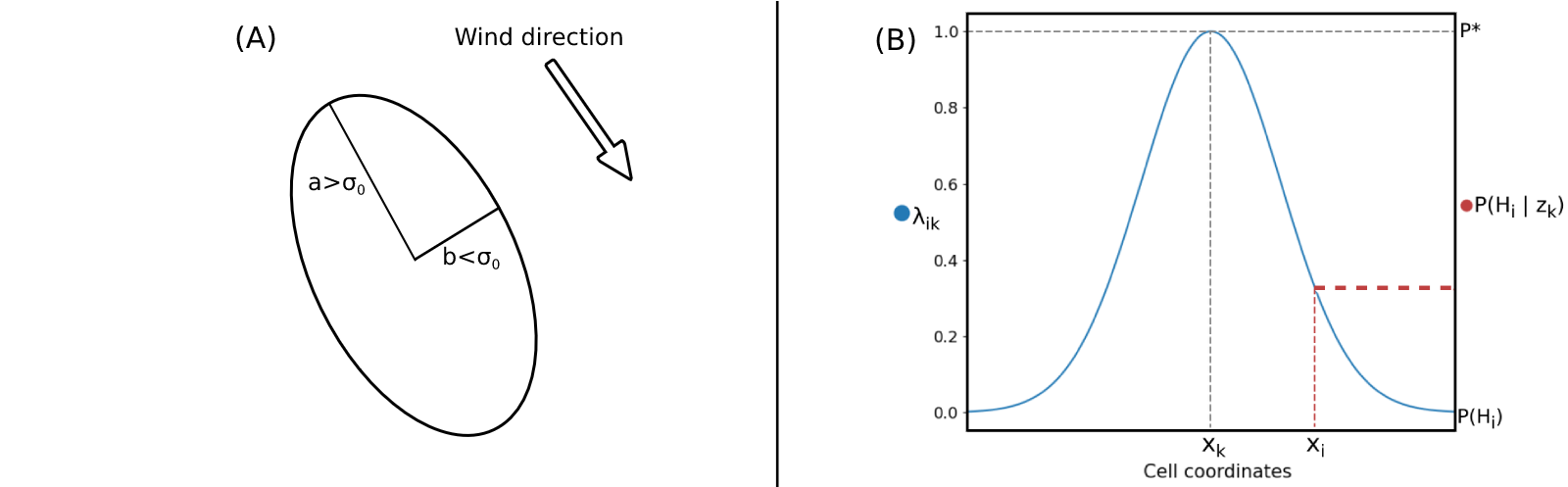
Figure 3: (A) The influence of a measurement ($\lambda_{i}$) over the probability of $H_{i}$ is calculated by sampling a 2D gaussian kernel of initial $\sigma=\sigma_{0}$, centered on the measurement location, that is stretched and rotated by the wind vector. The values of $a$ and $b$ are calculated using the method outlined in [21]. (B) One-dimensional simplification of the relation between $\lambda_{ik}$ and $P(H_{i}|z_{k})$, as described by equation  3.

While combining GDM and GSL is not a new idea, it is worth discussing in which ways our current proposal deviates from the conventions and techniques of GDM methods, and the reasoning behind these modifications. The main difference is that, rather than building a grid map of gas concentration values (a continuous random variable), we build a grid map of binary values, where a cell can either contain a measurable amount of gas (a gas hit) or not (a miss), and the exact concentration value is abstracted away. This presence of gas is treated as a random variable, and so we will deal with it in terms of the probability of a cell containing gas. Similarly to the Occupancy Grid Maps (OGM) employed in mobile robotics[22], the value at each grid cell represents the probability that the cell contains enough gas to trigger a gas detection event at an arbitrary instant of time.

From a frequentist perspective, these hit probabilities can be interpreted as the proportion of time that a cell contains enough gas to trigger a hit. Notice that this concept resembles the idea of plume mapping defined by Farrell et al. in [23], as this probability may be seen as the degree to which each cell belongs to the shape of the time-averaged gas plume: some cells are ”stably in the plume” (i.e. always contain a concentration of the target gas above a minimum threshold), while others are only partially so, as fluctuations in the shape of the plume can cause them to not contain gas at certain times.

The reason abstract away the concentration values is to better match the degree of precision that is attainable with predictive dispersion models –particularly during an online search, where many of the relevant parameters (boundary conditions, source release rate, etc) are uncertain. In this context, the comparison of specific concentration values measured by the sensor with those simulated by the dispersion model is not meaningful, as the simulations cannot be expected to match reality to such a degree of accuracy. Working at a higher level of abstraction attenuates the impact of these limitations –for example, the general shape of a gas plume, as represented by the gas hit variable, is largely independent of the release rate of the source, while the concentration values would greatly depend on it.

Formally, a gas-hit map is defined as a vector of binary random variables, $H=\{H_{i}|i\in C\}$, where $C$ is the set of all cells in the environment. We will refer to the set of sensory observations as $Z$, using a subscript to denote the position at which the observation was taken and a superscript to denote the time instant (e.g. $z_{k}^{t}\in Z$ is the observation taken at time $t$ in cell $k$). These superscripts and subscripts will be omitted for the sake of readability when they are not relevant to the discussion. We will refer to the probability of cell $i$ containing enough gas to trigger a gas hit as $p(H_{i})$.

III-B Building the Gas Hit Map

The estimation of the gas-hit map –$p(H_{i}|Z)\forall i$– is carried out recursively by bayesian filtering. Starting from an arbitrary prior $p(H_{i})$, each measurement taken in cell $i$ will modify the estimated probability of $H_{i}$ through the conditional probability $p(H_{i}|z_{i})$. We can define this conditional probability as a piece-wise function that depends on whether the observation is a hit or a miss:

$$p(H_{k}|z_{k})=P^{*}\begin{cases}=P_{hit}\text{, if }z_{k}=1\\ =P_{miss}\text{, if }z_{k}=0\end{cases}$$ (1)

Because of the complexity of the gas dispersion phenomenon, there is no clear way of setting grounded values for $P_{hit}$ and $P_{miss}$, thus they are left as input parameters to the algorithm, with the only requirement that

$$P_{hit}=p(H_{k}|z_{k}=1)>p(H_{k})$$

and

$$P_{miss}=p(H_{k}|z_{k}=0)<p(H_{k})$$

Interested readers can find a similar solution for occupancy mapping in [24, p. 33-35]. In that work, the author provides a solid discussion on arbitrarily defining conditional probabilities for a binary random variable given sensory observations.

Eq. 1 defines the conditional gas-hit probability of a cell only for a measurement taken in the same cell. Building a hit probability map only from this information would require an unfeasible amount of measures. Thus, some kind of inference to neighboring cells is required. For that, we resort to the wind vectors and the known geometry of the environment to compute an estimation of $p(H_{i}|z_{k})$ when $i\neq k$, so a map can be built from sparse measurements.

Intuitively, a hit measured at any specific cell should have no effect on the hit probability of far-away cells, but must change the probability of their surrounding cells according to their distance and position. Concretely, cells that are located upwind or downwind from the measurement location should be more strongly affected, as a noticeable airflow causing advection will create a stronger correlation between the state of cells whose relative position aligns with the wind vector.

Several methods have been proposed in the field of GDM to encode this dependency between cells based on distance and airflow alignment. In this work, similarly to the Kernel DM+V/W method [25], we apply a dependency model given by a 2D Gaussian centered at the measurement location and aligned with the wind vector. Thus, the influence factor $\lambda_{ik}$ of a measurement taken in cell $k$ over the conditional probability of $H_{i}$ is given by:

$$\lambda_{ik}\propto\mathcal{N}({x_{i}};{x_{k}},\Sigma)$$ (2)

where ${x_{i}}$ stands for the coordinates of any cell $i$, ${x_{k}}$ are the coordinates of the cell in which the measurement is taken, and $\Sigma$ is the covariance matrix of the 2D Gaussian, stretched and rotated according to the wind vector as described in [25] (see Fig. 3A). The value of $\lambda_{ik}$ is scaled by $1/N({0},\Sigma)$ to set the maximum value of the influence (when $i=k$) to 1.

We use this influence value $\lambda_{ik}$ to linearly interpolate between two extreme cases for $p(H_{i}|z_{k})$ following the expression:

$$p(H_{i}|z_{k})=\lambda_{ik}\cdot P^{*}+(1-\lambda_{ik})\cdot p(H_{i})$$ (3)

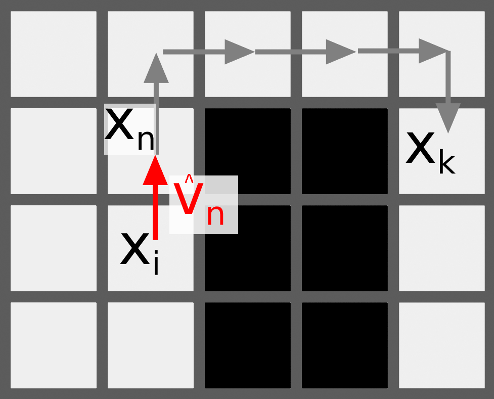
Figure 4: The vector $\hat{v}_{n}$ used in expression 4 is the direction from the considered cell $i$ to the cell $n\in N$ that is part to the shortest path between $i$ and $k$. $\delta_{ik}$ is the total length of said path.

When $i=k$ (the cell is being directly observed), $\lambda_{ik}=1$ and we are applying the expression  1. When the cell $i$ is very far away from cell $k$, $\lambda\approx 0$ and $p(H_{i}|z_{k})=p(H_{i})$, meaning that $H_{i}$ and $z_{k}$ can be considered independent (see Fig. 3B).

III-C Obstacles

An additional consideration is required for this method to be applicable to real scenarios where obstacles (walls, furniture, etc.) may exist between cells $i$ and $k$. This issue can be addressed by modifying the calculation of $\lambda_{ik}$ in such a way that its value is not based on the relative positions of cell $i$ and $k$, but rather on the direction and length of the shortest free path between them [26]. To efficiently find these paths, we employ the propagation method described in [16].

As a brief overview, the method is based on treating the grid of cells as a graph, where each free cell (i.e. not occupied by an obstacle) is a vertex, and two vertices are connected if their corresponding cells are both free and neighboring each other. On this graph we apply a search technique based on Dijkstra’s algorithm, starting from the set of cells that are neighboring the robot’s position ($N$) to find all the cells in the grid which should be assigned to each of the members of $N$ based on traversable distance. The result of this can be seen as a graph partition, where each group of vertices $G_{n}$ is defined by the vertex $n\in N$ which is closest to all the members of the group.

Based on this graph partition and the paths calculated in the process of creating it, we can redefine the value of $\lambda_{ik}$ for a cell $i\in G_{n}$ as:

$$\lambda_{ik}\propto\mathcal{N}(\hat{v}_{n}\delta_{ik};\text{ }{x_{k}},\Sigma)$$ (4)

where $\hat{v}_{n}$ is the vector $({x_{n}}-{x_{k}})$ normalized by its length (i.e. unit vector from $x_{k}$ to $x_{n}$) and $\delta_{ik}$ is the length of the shortest path connecting $i$ to $k$ (see Fig. 4). Note that this expression becomes the expression 2 for cells in the immediate vicinity of the robot, but will produce slightly different results for cells that are further away even if no obstacles exist along the path, as the direction of $\hat{v}_{n}$ might not perfectly line up with $({x_{i}}-{x_{k}})$. Implementations of this algorithm may choose to add an extra check for this case and apply expression 2 whenever a direct line of sight exists, but our testing shows no difference in the effectiveness of the algorithm in either case.

III-D Bayesian Update

We have so far omitted the time superscript on the measurements, and described only the conditional probability of $p(H_{i}|z_{k}^{t})$, for a single measurement $z_{k}^{t}$. However, the actual estimation of the map of hit probabilities is based on combining the information obtained from all the accumulated measurements. This process can be done recursively through Bayesian filtering, where we consider the conditional probability discussed in the previous sections, $p(H_{i}|z^{t})$, as the inverse sensor model.

Since the variable $H_{i}$ we are interested in when building the map is a binary random variable, we can use the log-odds form of the binary Bayes filter [22]:

$$l(H_{i}|z^{1:t})=l(H_{i}|z^{1:t-1})+l(H_{i}|z^{t})-l(H_{i})$$ (5)

where $l(x)$ denotes the log-odds:

$$l(x)=\frac{p(x)}{1-p(x)}$$

and the actual probability value can be recovered with:

$$p(x)=1-\frac{1}{1+e^{l(x)}}$$

III-E Confidence Value

An important consideration when using the generated hit probability map to estimate the location of the source is that the hit probability values that are estimated at some locations are based on measures in the near vicinity of that cell, while others are only due to extrapolation, or even still equal to the uninformative prior. Trivially, the estimations about the presence of gas that are based on extensive observations should have a stronger effect over the predicted source location probabilities.

Thus, it becomes necessary to quantify the uncertainty about the hit probabilities at each cell, which can be defined as a function of how many measurements have been gathered, and how close to the cell those measurements were taken. In this work, we will use the confidence measure $\alpha$ introduced in [21], which is calculated as follows:

$$\Omega_{i}=\sum_{t}\mathcal{N}(\delta^{t};0,\sigma)$$

$$\alpha_{i}=1-e^{-\Omega_{i}^{2}/\sigma_{\Omega}^{2}}$$ (6)

where $\delta^{t}$ is the length of the shortest path between $x_{i}$, (the position of the cell being updated), and $x_{z}^{t}$ (the position at which the robot took a measurement at timestep $t$). Both $\sigma$ and $\sigma_{\Omega}$ are parameters that control how much confidence is gained from each individual measurement. For more information about these parameters, see [21].

IV Source Position Estimation

In this section, we will discuss the process of using the map of $p(H_{i}|Z)\forall i$ that was built from the measurements to generate an estimation of the position of the source.

IV-A Hit Map Comparison

We define a random variable $S$ to represent the source location as a discrete variable whose possible values are each of the free cells in the environment. The probability distribution that we want to calculate is thus $p(S|H)$.

As explained in section III, the core idea of our proposal is that we can estimate the probability of a certain cell being the source location by comparing the plume that would result from having the source there (according to a dispersion model), to the plume we have constructed from measurements. Specifically, when we talk about ”comparing the plumes”, we mean comparing the hit probabilities, where these probabilities can be understood as relative frequencies. We define $f^{z}_{i}=P(H_{i}|Z)$ and $f^{S_{k}}_{i}=P(H_{i}|S_{k})$ as these predicted relative frequencies given the measurements and given the predictive model for a source in cell $k$, respectively. The absolute difference between these two values, $\Delta_{ik}$, can then be used as a measure of the similarity between the measured and the predicted states of cell $i$:

$$\Delta_{ik}=|f^{z}_{i}-f^{S_{k}}_{i}|$$ (7)

We can then define the conditional probability of $S$ with the following expression:

$$p(S_{k}|H_{i})\propto\alpha_{i}\cdot(1-\Delta_{ik})+(1-\alpha_{i})$$ (8)

When considering a $f^{z}_{i}$ that is based on a very low confidence ($\alpha_{i}$) estimation, the probability distribution of the source is uniform. As $\alpha_{i}$ approaches 1, the probability distribution of the source favors the locations which predict a value of $f^{S_{k}}_{i}$ similar to $f^{z}_{i}$.

Assuming conditional independence of each $H_{i}$ given $S$, the probability distribution of the source is then calculated as:

$$p(S_{k}|H)=\prod_{i}\frac{p(S_{k}|H_{i})\cdot p(H_{i})}{p(S_{k})\cdot p(H_{i}|H_{\neg i})}=\\ \prod_{i}p(S_{k}|H_{i})\cdot\prod_{i}\frac{p(H_{i})}{p(S_{k})\cdot p(H_{i}|H_{\neg i})}$$ (9)

where $H_{\neg i}$ denotes the set $\{H_{j}|j\neq i\}$. If we assume the prior probability distribution of the source location to be uniform, the term $\prod_{i}\frac{p(H_{i})}{p(S_{k})\cdot p(H_{i}|H_{\neg i})}$ is equal for all $k$, and since we assume there is a single gas source, we can simply omit it from the calculation and normalize the resulting values to obtain a valid probability distribution:

$$p(S_{k}|H)\propto\prod_{i}p(S_{k}|H_{i})$$ (10)

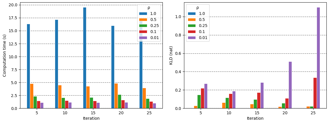
Figure 5: Effect of modifying the fraction of cells that are subdivided on each coarse-to-fine step ($\rho$). (A) Computation time. (B) Kullback-Leibler divergence of the resulting source location probability distribution with respect to the distribution predicted by considering all the cells.

IV-B Filament model

The formulation discussed in the previous section requires a predictive gas dispersion model that, given a source position, produces a map of hit probabilities for the expected gas plume. Because of the types of environmental conditions that we are considering (indoor environments with obstacles), we opt for a simplified version of the filament model.

In the original filament model, as proposed by Farrell et al [17], the dispersion of gas is simulated by tracking the movement of discrete units (the filaments), which in turn represent three-dimensional spatial distributions of concentration –usually modeled as normal distributions centered on the filament’s position. The filaments are assumed to move mostly through advection, and the effects of diffusion are accounted for by changing the parameters of the concentration distribution that each filament represents. That is, a filament that was emitted a long time ago represents a normal distribution of higher $\sigma$ than one that was just released from the source, even though both distributions contain the same number of moles of the realized gas.

For the purposes of this work, the filament model has been simplified in two ways. The first and most important one is that the simulation takes place in two dimensions rather than three. This is partially to alleviate the computational complexity of the proposed method, but also to account for the fact that only 2D airflow information is available from the GMRF estimations.

The second way in which our implementation deviates from the filament model is that, since we are not interested in computing concentration values (for the reasons discussed in section III), we are not modeling the filaments as normal distributions of concentration. Instead, we consider that filaments have a discrete radius that grows as a function of the length of time that has passed since their emission. During the simulation, we record the number of time instants that each cell is close enough to the position of at least one filament to be occupied by gas. The relative frequency of this event is the value of $f^{S_{k}}_{i}=P(H_{i}|S_{k})$.

IV-C Iterative Coarse-to-Fine Refinement

Despite the adoption of a simplified model, the filament model still has a significant computational cost, as a complete simulation needs to be carried out for each cell in the environment. In order to alleviate this computational load, some optimizations can be implemented so that a higher proportion of the time is spent on the calculations that will significantly impact the algorithm’s predictions about the source location.

Consider, for example, a simulation with the source in cell $i$ whose predicted plume map does not match at all the measurements that have been taken so far. It is trivial that simulations with the source in the immediate neighbors of $i$ will produce similar plumes, which will also be poor matches for the real measurements, and thus those cells will be evaluated as unlikely source locations. On the contrary, areas of the map that are evaluated positively benefit much more from increased resolution, as it may be required to differentiate from several likely source candidates. We propose to utilize this idea by employing a progressive refinement (coarse-to-fine) strategy, where only a few source locations are simulated initially as representatives of coarse regions, and those regions which produce the most promising results are recursively subdivided to obtain more precision in the final estimations.

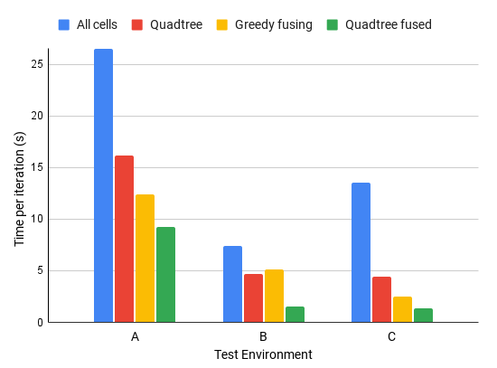
Figure 6: Average time required to update the source position distribution with the discussed optimizations in three different environments, with $\rho=0.5$

We refer to the proportion of cells that gets subdivided in each successive step of this process as the refinement fraction ($\rho$). Figure 5 shows how $\rho$ affects the computation time and the quality of the resulting estimation as the search process progresses. The quality of the estimation is measured as the Kullback-Leibler divergence between the probability distribution of $S$ obtained with that refinement fraction, and the probability distribution of $S$ that results from considering all cells. Note that the KLD for $\rho=1$ is trivially always 0, as its resulting probability distribution is the one being approximated.

It can be observed that for $\rho>0.25$ the KLD becomes negligible as the number of iterations of the algorithm advances. Conversely, the results obtained with a very small refinement fraction worsen over time. This effect is caused by the variance of the source’s distribution decreasing. As the search advances, a small number of nearby cells accumulate most of the probability of containing the source. When this happens, subdividing that small area of the map with a high probability of $S$ is enough to obtain a probability distribution very close to the one being approximated. For very small refinement fractions, the KLD increases because $P(S_{k}|H)$ can vary more drastically for nearby cells at this stage of the cell than when only part of the map has been observed, and thus the very limited amount of subvidisions is not enough to capture the high-frequency variations in the estimated probability of the source location.

We tested two different methods for generating these regions, both of which produce rectangular cells and allow for a maximum cell size to be specified to make sure the regions are not so coarse as to have the environmental conditions change significantly inside of them. The first method is to generate a quadtree from the occupancy map, which allows for large unoccupied regions to be grouped together into a single leaf of the tree, while allowing obstacles to serve as boundaries that force areas to be considered separately. The second method is to greedily fuse the free cells in the occupancy map with their neighbors, in an arbitrary order, with the only constraint being that the resulting cells must remain rectangular. While both of these methods allowed for a significant speed increase from the naive approach (see Figure 6), the biggest speedup was obtained by combining both: generating a quadtree, and then fusing the resulting neighboring leaves.

Note that none of these methods are guaranteed to generate an optimal number of subdivisions of the map according to our constraints. A more in-depth study of this problem is left for future work.

V Movement Strategy

One of the most common strategies for planning the movements of the robot is to maximize the information about the source location that is gained with each new measurement. This idea has been extensively explored by previous methods, in what is usually referred to as ”information-theoretic” movement strategies. One of the most notable examples of this idea is Infotaxis [27], which popularized the use of the expected change in the entropy of the source distribution as a measure for the information gain. Later works [28, 16] have proposed using the Kullback-Leibler Divergence instead, since aiming only to decrease entropy can cause the robot to refuse exploration and only focus on confirming its current belief.

All of these approaches have a common problem: they require estimating what the next measurement will be if the robot moves to a given position. With this hypothetical next measurement, they simulate an update on the source position belief, and compare the result to the current one. This requires a method for reliably estimating what the next measurement will be, which is not trivial and also requires performing an iteration of the source estimation procedure for each considered movement, which can lead to a prohibitive computational cost if the number of possible movements is large. Since our algorithm has a slow update process, requiring many filament simulations, this approach is not feasible.

(a)

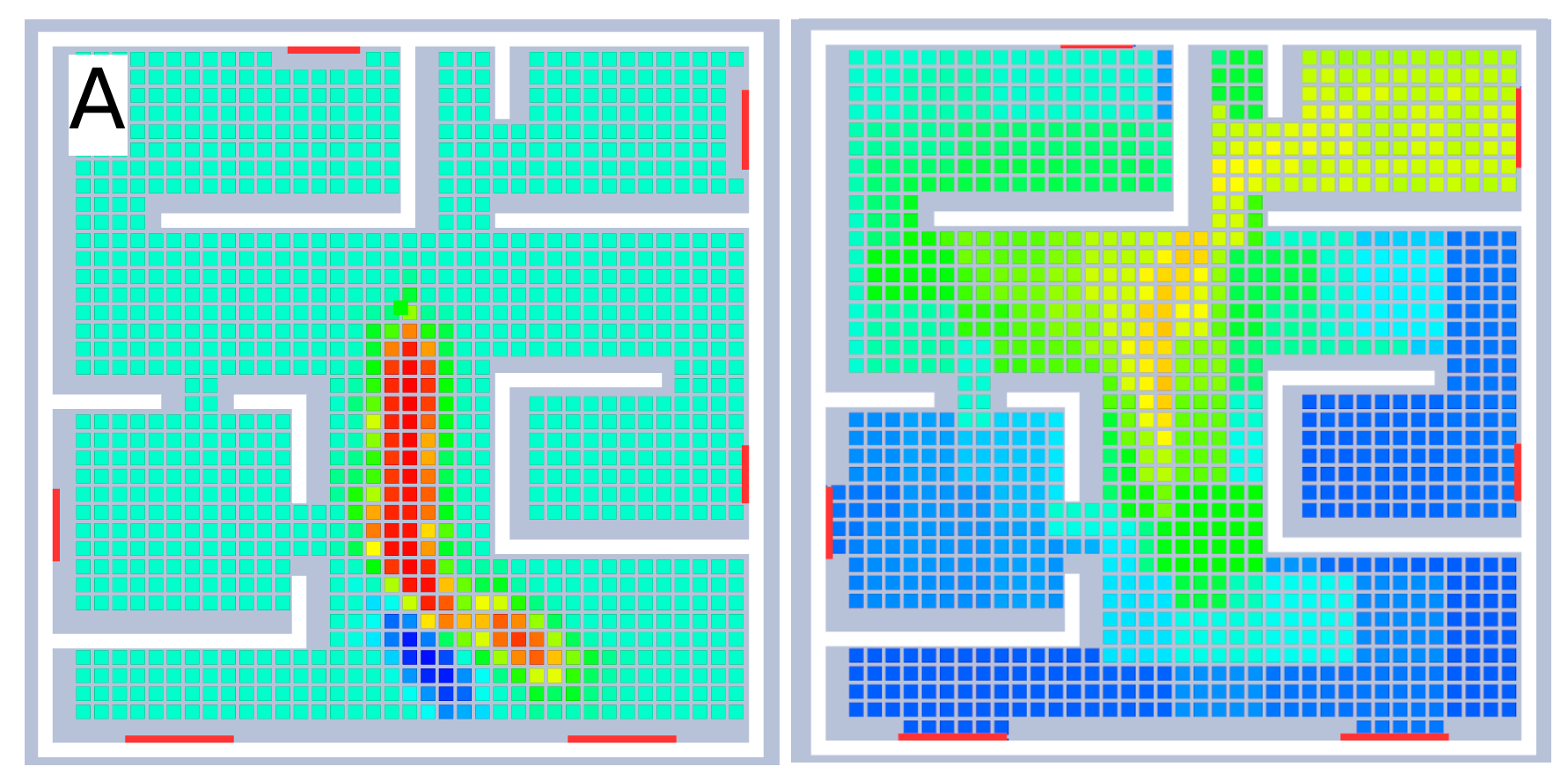
(b)

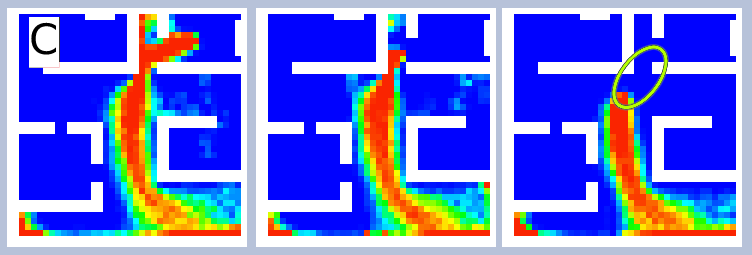
Figure 7: The movement strategy tries to maximize information about the source location by visiting the locations where the expected plumes vary the most. (A) Current hit probability map. (B) Current source probability distribution. (C) Examples of the maps generated by the dispersion model for the most likely source locations. The area marked with an ellipse changes the most between these maps, so it is chosen as the next measurement location.

Instead, we propose using the already-computed filament simulations to identify the most interesting areas. When trying to discriminate between two possible source positions, the areas of most interest for taking measurements are those in which their respective predicted plumes are most different (see Figure 7). We generalize this to all possible source positions and use their estimated probabilities of containing the source as a weight for how much their prediction influences the interest of a measurement location. This is represented by the variance of $p(H_{i}|S)$. If we include the term $(1-\alpha_{i})$, so that areas that have already been observed extensively are considered less interesting, the information value of a particular measuring location, $\psi$, is therefore calculated as follows:

$$\psi_{i}=(1-\alpha_{i})\cdot\sum_{k}p(S_{k})\cdot(p(H_{i}|S_{k})-\mu_{i})^{2}$$ (11)

$$\text{with }\mu_{i}=\sum_{k}p(H_{i}|S_{k})\cdot p(S_{k})$$

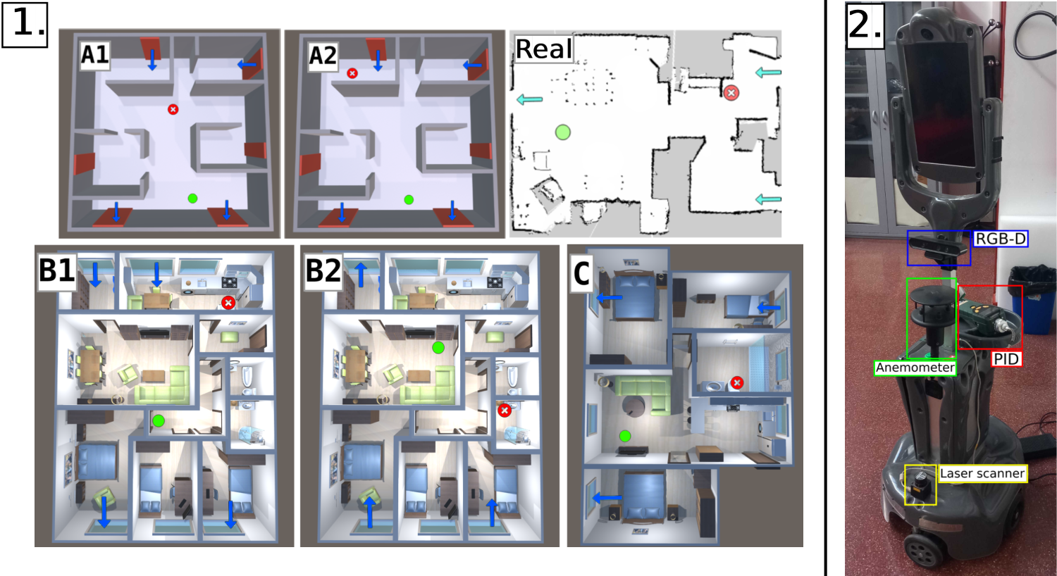
Figure 8: The simulated scenarios. The starting position of the robot is marked with a green circle and the source location with a red circle with a cross. The blue arrows signal the inlets and outlets for the airflow.

VI Experimental Validation

The experimental validation of the proposed algorithm was carried out by performing both simulation and real-world testing. The benefit of using simulation is that it allows for easily repeatable experimentation under a wide range of scenarios and conditions, while the real-world experiments serve to verify that the results obtained in the simulations still hold under real, uncontrolled conditions. All configuration files for these experiments (both simulated and real), which include the input parameters of the algorithm, can be found on an online repository .

VI-A Setup

For the simulations, we rely on GADEN [18], a 3D gas dispersion simulator that employs CFD-based airflow. We tested the algorithm’s performance under five different scenarios, taking place in three distinct environments (Fig. 8). The first environment is a simplified version of a generic indoor location, featuring multiple rooms and walls, but no limited-height obstacles to fully explore the three-dimensionality of the gas dispersion process. The other two environments are models of real houses, and the specific scenarios considered have been selected from the VGR dataset [29]. Experiments A1 and A2 (and, similarly, B1 and B2) take place in the same environment, but with a different configuration –i.e., the source is placed at a different location and/or the airflow inlets and outlets have changed.

We compare the currently presented algorithm (labeled in the results as PMFS) to the algorithm presented in [16], (labeled GrGSL). Each of the experiments comprised 30 runs for each of the algorithms, which are considered to end once the variance of the probability distribution of the source location falls below a fixed threshold –in this case, $1m^{2}$.

The real-world experiments were carried out inside a house, using natural ventilation as the sole source of airflow. The gas source was an ultrasonic vibration humidifier loaded with a 96% ethanol solution. We used a Giraff robot equipped with a photoionization detector (PID) and an ultrasonic anemometer for GSL, and with a laser scanner and RGB-D camera for navigation. Because these experiments are vastly more time-consuming to carry out, only 10 runs of each algorithm were recorded as a way to validate the more extensive simulation results.

VI-B Results

Results are shown in Fig. 9. The ”error” value displayed in Fig. 9 is the distance in meters between the ground-truth source location and the source position declared by the algorithm after reaching the convergence criterion. For these experiments, it is considered that the algorithm has converged on a solution when the variance of the source’s probability distribution falls below $1m^{2}$, following the results obtained in [30]. Figure 10 also shows the number of iterations required for the algorithm to reach this convergence criterion. Note that we report number of iterations, rather than total search time, because with the computation times reported in section IV-C, the vast majority of the time is spent on navigation. Since navigation time can greatly vary from one run to another, and has a strong dependency on the movement scheme of the particular robot being used, iteration count offers more insight into the length of the search process.

It can be observed that the proposed method outperforms GrGSL in the more complex environments, while obtaining comparable results in the simpler cases. Experiment B2 proves to be particularly challenging, with both algorithms producing estimations that are, on average, more than 2m away from the actual source position. This shows one of the main limitations of our proposed method, which is that it very strongly relies on obtaining an accurate estimation of the direction of the airflow, and is unable to do so when the three-dimensionality of the environment plays an important role (Fig. 11 shows a stream trace of the airflow around the point where the source is placed). In other cases (see scenarios B1 and C), the new method is able to produce much better estimations than the previous algorithm, because GrGSL tends to produce an estimation that is as far upwind as possible inside the gas plume, while the reasoning of the new method (comparing the plume that would be produced if the source was in a specific location to the currently mapped plume) allows it to produce estimations that are not aligned with the airflow currents.

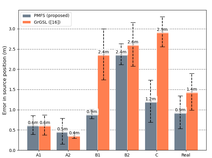
Figure 9: Average error in meters between the final estimated source location and the ground truth in each of the simulated scenarios.

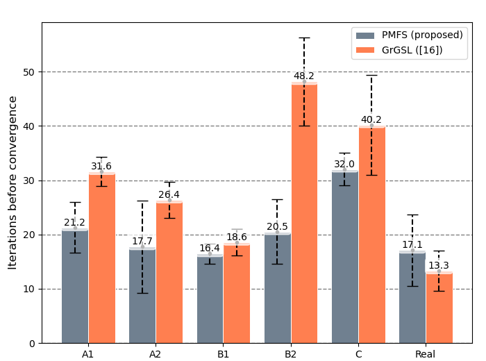
Figure 10: Number of iterations required for each of the algorithms to reach convergence, defined as a threshold on the variance of the source’s conditional probability distribution.

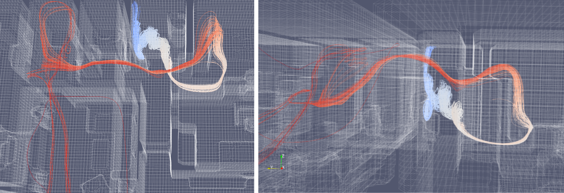
Figure 11: Stream trace of the airflow near the source position in scenario B2. The strong three-dimensionality of the dispersion process poses a challenge for the proposed method, since the dispersion model used by PMFS only considers two dimensions.

Figure 12: Snapshot of the calculated probabilities during the search in the real-world environment. (A) Hit probability map, with the arrows showing the estimated wind direction. (B) Source location probability distribution. The red arrow is the pose of the robot, and the blue lines indicate the measurements of the laser scanner.

The results obtained in the real-world experiment are coherent with what might be expected given the previous simulations. The complexity of the geometry of the environment is comparable to simulated scenario C, with the most notable difference being the placement of the source directly inside of the main air current, rather than inside of an adjacent room. This difference explains the significantly better results obtained by GrGSL, for the reasons discussed in the previous paragraph. It can be observed that both methods obtain comparable results, both in terms of the error in the final estimation, and in the number of iterations required to produce it. While the error recorded from PMFS is on average lower, the variance of the results and the lower repetition count of the real-world experiment compared to the simulations, make this relatively small difference not very meaningful. Figure 12 shows a snapshot of the probabilities calculated by PMFS (of each $H_{i}$, and of $S$) during the search. It can be observed that the area that receives the highest probability of containing the source is at the start of the plume (following it upwind), but that, given that many cells remain unobserved (with $P(H_{i}|Z)\approx P(H_{i})$ and $\alpha_{i}\approx 0$) there still exists significant uncertainty in $P(S|H)$.

VII Conclusions and Future Work

The gas source localization algorithm presented in this work revolves around the idea of using a forward gas dispersion model to estimate the gas plume that would be produced if the source was in a certain position, and comparing that prediction with the data that has been obtained so far.

The specifics of the model used and the calculations done with those results, as presented here, should not be considered a finalized solution, but merely a first attempt at making a feasible implementation of the concept. Indeed, many of the biggest limitations of the method (mainly those related to the 3D phenomena) could be addressed by using more robust, more accurate methods for the airflow estimation and the gas dispersion, although a compromise between accuracy and computational complexity will always be required to perform on-line simulations during the search.

Another limitation that should be addressed by future work is the need to know the map of the environment in advance. Developing methods for estimating the airflow and simulating the gas dispersion in partially observed environments with uncertainty would be of great importance in making the concepts presented here fit for real applications.

References

- [1] D. Karakaya, O. Ulucan, and M. Turkan, “Electronic Nose and Its Applications: A Survey,” International Journal of Automation and Computing, vol. 17, no. 2, pp. 179–209, 2020.
- [2] S. Feng, F. Farha, Q. Li, Y. Wan, Y. Xu, T. Zhang, and H. Ning, “Review on smart gas sensing technology,” Sensors (Switzerland), vol. 19, no. 17, pp. 1–22, 2019.
- [3] A. Francis, S. Li, C. Griffiths, and J. Sienz, “Gas source localization and mapping with mobile robots: A review,” Journal of Field Robotics, vol. 39, no. 8, pp. 1341–1373, 2022.
- [4] R. Visvanathan, K. Kamarudin, S. M. Mamduh, M. Toyoura, A. S. Ali Yeon, A. Zakaria, L. M. Kamarudin, X. Mao, and S. A. Abdul Shukor, “Improved mobile robot based gas distribution mapping through propagated distance transform for structured indoor environment,” Advanced Robotics, vol. 34, no. 10, pp. 637–647, May 2020.
- [5] A. Gongora, J. Monroy, and J. Gonzalez-Jimenez, “Joint estimation of gas and wind maps for fast-response applications,” Applied Mathematical Modelling, vol. 87, pp. 655–674, 2020.
- [6] X. xing Chen and J. Huang, “Odor source localization algorithms on mobile robots: A review and future outlook,” Robotics and Autonomous Systems, vol. 112, no. November, pp. 123–136, Feb. 2019.
- [7] Z. Li, Z. F. Tian, T. fu Lu, and H. Wang, “Assessment of different plume-tracing algorithms for indoor plumes,” Building and Environment, vol. 173, no. October 2019, pp. 106 746–106 746, 2020.
- [8] J. Macedo, L. Marques, and E. Costa, “A Comparative Study of Bio-Inspired Odour Source Localisation Strategies from the State-Action Perspective,” Sensors, vol. 19, no. 10, pp. 2231–2231, 2019.
- [9] F. Rahbar and A. Martinoli, “A Distributed Source Term Estimation Algorithm for Multi-Robot Systems,” Proceedings - IEEE International Conference on Robotics and Automation, pp. 5604–5610, 2020.
- [10] M. Hutchinson, H. Oh, and W. H. Chen, “A review of source term estimation methods for atmospheric dispersion events using static or mobile sensors,” Information Fusion, vol. 36, pp. 130–148, 2017.
- [11] J. R. Bourne, E. R. Pardyjak, and K. K. Leang, “Coordinated Bayesian-Based Bioinspired Plume Source Term Estimation and Source Seeking for Mobile Robots,” IEEE Transactions on Robotics, vol. 35, no. 4, pp. 967–986, 2019.
- [12] M. Park and H. Oh, “Cooperative information-driven source search and estimation for multiple agents,” Information Fusion, vol. 54, pp. 72–84, Feb. 2020.
- [13] H. Magalhães, R. Baptista, J. Macedo, and L. Marques, “Towards Fast Plume Source Estimation with a Mobile Robot,” Sensors, vol. 20, no. 24, p. 7025, Dec. 2020.
- [14] C. Sanchez-Garrido, J. Monroy, and J. Gonzalez-Jimenez, “Probabilistic estimation of the gas source location in indoor environments by combining gas and wind observations,” Frontiers in Artificial Intelligence and Applications, vol. 310, pp. 110–121, 2018.
- [15] M. Asenov, M. Rutkauskas, D. Reid, K. Subr, and S. Ramamoorthy, “Active Localization of Gas Leaks Using Fluid Simulation,” IEEE Robotics and Automation Letters, vol. 4, no. 2, pp. 1776–1783, Apr. 2019.
- [16] P. Ojeda, J. Monroy, and J. Gonzalez-Jimenez, “Information-Driven Gas Source Localization Exploiting Gas and Wind Local Measurements for Autonomous Mobile Robots,” IEEE Robotics and Automation Letters, vol. 6, no. 2, pp. 1320–1326, 2021.
- [17] J. A. Farrell, J. Murlis, X. Long, W. Li, and R. T. Cardé, “Filament-based atmospheric dispersion model to achieve short time-scale structure of odor plumes,” in Environmental Fluid Mechanics, vol. 2, 2002, pp. 143–169.
- [18] J. Monroy, V. Hernandez-Bennetts, H. Fan, A. Lilienthal, and J. Gonzalez-Jimenez, “GADEN: A 3D gas dispersion simulator for mobile robot olfaction in realistic environments,” Sensors (Switzerland), vol. 17, no. 7, pp. 1–16, 2017.
- [19] J. G. Li, Q. H. Meng, Y. Wang, and M. Zeng, “Odor source localization using a mobile robot in outdoor airflow environments with a particle filter algorithm,” Autonomous Robots, vol. 30, no. 3, pp. 281–292, 2011.
- [20] J. Monroy, M. Jaimez, and J. Gonzalez-Jimenez, “Online estimation of 2d wind maps for olfactory robots,” in International Symposium on Olfaction and Electronic Nose (ISOEN), 2017, pp. 1–3.
- [21] A. J. Lilienthal, M. Reggente, M. Trincavelli, J. L. Blanco, and J. Gonzalez, “A statistical approach to gas distribution modelling with mobile robots - the kernel dm+v algorithm,” in 2009 IEEE/RSJ International Conference on Intelligent Robots and Systems, 2009, pp. 570–576.
- [22] S. Thrun, W. Burgard, and D. Fox, Probabilistic Robotics, ser. Intelligent Robotics and Autonomous Agents series. MIT Press, 2005.
- [23] J. A. Farrell, S. Pang, and W. Li, “Plume Mapping via Hidden Markov Methods,” IEEE Transactions on Systems, Man, and Cybernetics, Part B: Cybernetics, vol. 33, no. 6, pp. 850–863, 2003.
- [24] R. S. Merali, “Benefits of Cell Correlations in Occupancy Grid Mapping,” Ph.D. dissertation, University of Toronto, 2020.
- [25] M. Reggente and A. J. Lilienthal, “Using local wind information for gas distribution mapping in outdoor environments with a mobile robot,” in Proceedings of IEEE Sensors. IEEE, Oct. 2009, pp. 1715–1720.
- [26] R. Visvanathan, K. Kamarudin, S. M. Mamduh, M. Toyoura, A. S. Ali Yeon, A. Zakaria, L. M. Kamarudin, X. Mao, and S. A. Abdul Shukor, “Improved mobile robot based gas distribution mapping through propagated distance transform for structured indoor environment,” Advanced Robotics, vol. 34, no. 10, pp. 637–647, May 2020.
- [27] M. Vergassola, E. Villermaux, and B. I. Shraiman, “’Infotaxis’ as a strategy for searching without gradients,” Nature, vol. 445, no. 7126, pp. 406–409, 2007.
- [28] M. Hutchinson, C. Liu, and W. H. Chen, “Information-Based Search for an Atmospheric Release Using a Mobile Robot: Algorithm and Experiments,” IEEE Transactions on Control Systems Technology, pp. 1–15, 2018.
- [29] P. Ojeda, J. Monroy, and J. Gonzalez-Jimenez, 2023 - Under review, data available online: https://mapir.isa.uma.es/mapirwebsite/?p=1708.
- [30] ——, “On gas source declaration methods for single-robot search,” in IEEE International Symposium on Olfaction and Electronic Nose (ISOEN), 2022, pp. 1–3.