Deep Collective Knowledge Distillation
Abstract
Many existing studies on knowledge distillation have focused on methods in which a student model mimics a teacher model well. Simply imitating the teacher’s knowledge, however, is not sufficient for the student to surpass that of the teacher. We explore a method to harness the knowledge of other students to complement the knowledge of the teacher. We propose deep collective knowledge distillation for model compression, called DCKD, which is a method for training student models with rich information to acquire knowledge from not only their teacher model but also other student models. The knowledge collected from several student models consists of a wealth of information about the correlation between classes. Our DCKD considers how to increase the correlation knowledge of classes during training. Our novel method enables us to create better performing student models for collecting knowledge. This simple yet powerful method achieves state-of-the-art performances in many experiments. For example, for ImageNet, ResNet18 trained with DCKD achieves 72.27%, which outperforms the pretrained ResNet18 by 2.52%. For CIFAR-100, the student model of ShuffleNetV1 with DCKD achieves 6.55% higher top-1 accuracy than the pretrained ShuffleNetV1.
1 Introduction
Knowledge distillation [8] is an effective method for compressing a heavy teacher model to a lighter student model. The main idea of knowledge distillation is that a teacher model with higher capacity and better performance distills the softened output distribution into a student model as knowledge. Hinton et al. [8] explained that softened outputs with higher entropy than hard labels provide much richer information. In previous studies [1, 8, 17], assigning the probabilities to other classes, which leads to increased entropy, was effective in generalizing a network. These probabilities provided valuable information about the correlation between other classes and Dubey et al. [4] showed that maximum entropy training with these correlation information is effective. Many studies [18, 10, 15, 16, 7, 14, 21, 24] on knowledge distillation have focused on efficiently transferring teacher’s knowledge to students. We took a step further by adopting a different approach to knowledge enrichment. If a student model learns from only a teacher’s soft targets, then the student will only imitate the teacher. However, if the knowledge of peer students is additionally given, it can help a student model outperform the student model learned only from a teacher. Our work focuses on creating a student model that can have rich representation by training not only with the knowledge provided by the teacher but also with additional knowledge of various correlations between classes provided by the peer students. As a method for generating additional knowledge, we propose gathering knowledge from multiple students.
Mutual learning methods [2, 5, 12, 26] aim to train powerful student models using ensembled knowledge of multiple untrained students without a pretrained teacher model. These methods train multistudent models with knowledge generated on-the-fly from students’ logits, and this online knowledge is often generated to better represent the ground truth or soft targets of the teacher model. However, we propose an approach for generating additional online knowledge containing diverse correlation information from multistudent models, not similar to the ground truth or the teacher’s soft targets. Since the teacher model learned with the supervised learning manner becomes over-confident [20], it may overlook other correlation information. Thus, we believe that the additional knowledge, including correlational information between classes, can assist the teacher model.
We present deep collective knowledge distillation (DCKD) to improve the performance of a student model with a wealth of knowledge. Our method achieves state-of-the-art performances in every experiment. We perform extensive experiments on KD benchmarks on several datasets, including ImageNet [3], CIFAR-100, CIFAR-10 [11] and Fashion-MNIST [22]. For CIFAR-100, the student model of ResNet32 with DCKD achieves 3.83% higher top-1 accuracy than the pretrained ResNet32. Our two main contributions to this research are as follows: We design a novel method for constructing the additional knowledge collection with more correlation information between classes. We analyze and modify the collection loss between each student and knowledge collection by reversing the direction of Kullback-Leibler divergence.
2 Related Works
Knowledge Distillation The work of Hinton et al. [8] has revolutionized the literature of model compression by distilling the knowledge of a large model to a smaller model to construct a compact model. Hinton et al. [8] explained that the distribution of a teacher network, which is smoothed using temperature, can more clearly represent secondary probabilities. These secondary probabilities convey information about the correlation between labels and are crucial for teaching student networks. AT [24] attempted to improve knowledge distillation by including the effects of attention in models. FitNet [18] expected to mimic the teacher model by transferring the intermediate representation to the student model. FT [10] used paraphrased factors compressed from the teacher’s features to train the student, and RKD [14] utilized structural relations of data. OFD [7] proposed a feature distillation method, including a feature transform to keep the information of the teacher’s features. CC [15] focused on the correlation between the instances to transfer, and CRD [21] demonstrated how to make the student’s representation more similar to the teacher’s representation using a contrastive objective. ReviewKD [16] proposed a review mechanism that transfers multi-level knowledge of the teacher to one-level of the student.
Mutual Learning We provide DCKD as a novel approach for knowledge distillation, but our work is also related to mutual learning methods because multiple student models train each other. Deep mutual learning (DML) [26] trained multiple initialized models to gain remarkable performance without any pretrained teacher. ONE [12] ensembled logits of multiple students to generate an on-the-fly teacher and trained each student with it. OKDDip [2] similarly constructed an ensemble with students but considered attention-based weights for each student. KDCL [5] regarded all networks as students, proposed methods to generate a soft target from all these students, and mentioned that the generated soft target is transferred to all students as knowledge. The existing methods [12, 5] ensemble the outputs of each student to generate a single soft target and use it to train the students with the forward direction of Kullback-Leibler divergence. However, our method differs from these methods because our method trains each student with several different soft targets generated from different peers. Each student has more diversity by learning other students’ collective knowledge that does not include the individual knowledge of each student.


3 Method
3.1 Deep Collective Knowledge Distillation
Our method is based on the idea that a model can be a better student if the model’s output represents not only the distribution of the correct class but also a relationship with other classes, as Hinton et al. described [8]. For example, we assume that there is input data of the first class, which has features that are similar to the input data of the second class. If a model’s output has a one-hot distribution, e.g., , it only has information about the correct class and does not have any knowledge concerning other classes. On the other hand, if a model’s output distribution is , it can be considered that the input data is an object of the first class and shares some similarities with the input data of the second class. The similarities among the input data between two classes can help a student better learn the features of the input data.
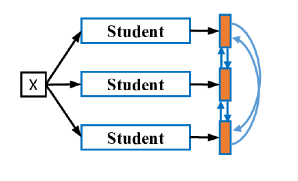
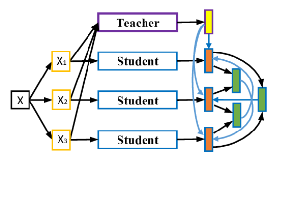
As shown in Fig. 1(c), each student is trained using the knowledge distillation loss with the teacher’s knowledge and using the collection loss with the collective knowledge constructed from other students, excluding oneself. After the training is finished, all students are independently utilized for the inference phase.
For a better mathematical definition, we denote the set of models as . Let be an input data chosen from dataset and be logits of a model, e.g., , where is a class index. We define logits and probability distribution as follows:
| (1) | ||||
| (2) |
We note that outputs logits instead of probability distribution . is the probability distribution of the -th student, and is typical softmax activation function.
Loss function With the definition of and , we state the -th student’s loss as
| (3) | ||||
| (4) | ||||
| (5) |
where represents a hard label, is the distribution of the teacher model’s output, is the set of the distribution of all student models’ outputs and is the distribution of the -th student’s output. Each is a constant weight for balancing each loss.
is composed of the following three parts: cross-entropy loss , knowledge distillation loss and collection loss . First, is a typical loss for a classification task. Second, the standard is defined as follows:
| (6) |
where and are logits of and , respectively. The temperature parameter softens the teacher’s output distribution, which is similar to the one-hot distribution, to obtain the higher entropy distribution with apparent secondary probabilities. Last, works as a bridge between each student and each collective knowledge. To compare two distributions, is based on the Kullback-Leibler divergence (KLD) and applies it in the reverse direction. To effectively conserve and transfer the correlation information, we construct as follows:
| (7) |
and are defined as follows:
| (8) |
where is a temperature parameter for . We will discuss more thoroughly in the following section.
Last, we state the total loss for training DCKD’s students:
| (9) |
We do not separately train the -th student by calculating the gradients of each ; rather, we simultaneously train every student with the gradients of . The main difference between the separate training and the simultaneous training is that the simultaneous training optimizes both distributions in , while the separate training optimizes only.
Collection methods We consider three methods for collecting knowledge to efficiently preserve the correlation between classes: logit max collection, probability max collection and average collection. Each collection method is utilized to find and is defined as follows:
-
•
Logit max collection
(10) -
•
Probability max collection:
(11) -
•
Average collection:
(12)
In these equations, and are applied in each class index of .
and collect max values from each class in students’ logits, whereas considers the max values as noise and cancels out by applying the average function for each class. From our point of view, the max collection method conveys more correlations between classes, while the average collection method erases these information. Thus, when we collect knowledge from several student models, the max collection method generates the distribution, which has rich information, while the average collection method generates the distribution, which is similar to the one-hot distribution.
The main difference between and is whether applies to logits or the distribution . is equal to if of is normalized to the same level by the following equation: . Therefore, focuses on the relative values of probabilities, whereas focuses on the absolute values of the logits. These collection methods are promising in theory, so we performed experiments to compare these methods. Empirically, performed better, so we adopted to gather knowledge from multiple students.
| Accuracy | Teacher | Student | KD | AT | CC | OFD | CRD | CRD+KD | ReviewKD | DCKD | ||
| [8] | [24] | [15] | [7] | [21] | [21] | [16] | Net1 | Net2 | Net3 | |||
| Top-1 | 73.31 | 69.75 | 70.06 (0.11) | 71.55 (0.16) | 71.45 (0.08) | 71.35 (0.03) | 71.89 (0.07) | 72.03 (0.01) | 72.24 (0.05) | 72.27 (0.06) | 72.11 (0.07) | 72.09 (0.06) |
| Top-5 | 91.42 | 89.07 | 89.99 (0.05) | 90.46 (0.15) | 90.21 (0.03) | 90.28 (0.04) | 90.59 (0.07) | 90.85 (0.04) | 90.86 (0.08) | 90.93 (0.03) | 90.95 (0.03) | 90.95 (0.03) |
| Teacher Network (Accuracy, %) | WRN-40-2 (76.35) | WRN-40-2 (76.35) | ResNet56 (73.23) | ResNet110 (74.36) | ResNet110 (74.36) | ResNet32x4 (79.54) | VGG13 (74.93) |
| Student Network (Accuracy, %) | WRN-16-2 (73.32) | WRN-40-1 (71.83) | ResNet20 (69.28) | ResNet20 (69.28) | ResNet32 (71.50) | ResNet8x4 (72.83) | VGG8 (70.92) |
| Method | Accuracy (std.) | ||||||
| KD [8] | 75.78 (0.09) | 74.62 (0.19) | 71.90 (0.43) | 72.14 (0.20) | 74.24 (0.09) | 73.49 (0.29) | 73.81 (0.12) |
| FitNet [18] | 73.72 (0.25) | 72.48 (0.07) | 69.09 (0.24) | 69.41 (0.16) | 70.73 (0.12) | 73.24 (0.11) | 71.35 (0.09) |
| AT [24] | 74.23 (0.17) | 73.42 (0.02) | 70.90 (0.03) | 70.96 (0.11) | 72.80 (0.25) | 73.86 (0.06) | 71.89 (0.26) |
| RKD [14] | 73.97 (0.32) | 72.70 (0.18) | 70.92 (0.25) | 70.54 (0.31) | 72.65 (0.11) | 71.75 (0.18) | 71.44 (0.07) |
| FT [10] | 73.69 (0.26) | 72.14 (0.03) | 70.77 (0.29) | 70.91 (0.13) | 72.36 (0.47) | 73.53 (0.07) | 71.29 (0.29) |
| CC [15] | 73.38 (0.18) | 72.05 (0.41) | 70.20 (0.31) | 69.76 (0.17) | 71.58 (0.02) | 72.65 (0.16) | 70.52 (0.10) |
| OFD [7] | 75.32 (0.32) | 74.21 (0.15) | 71.48 (0.13) | 71.59 (0.13) | 73.25 (0.20) | 74.35 (0.08) | 71.13 (0.10) |
| CRD [21] | 76.08 (0.09) | 74.68 (0.22) | 72.39 (0.30) | 72.28 (0.24) | 74.19 (0.10) | 75.61 (0.07) | 73.80 (0.16) |
| CRD+KD [21] | 76.08 (0.12) | 75.50 (0.14) | 72.67 (0.11) | 72.66 (0.09) | 74.72 (0.15) | 75.49 (0.10) | 74.37 (0.07) |
| ReviewKD [16] | 75.75 (0.07) | 74.90 (0.15) | 71.93 (0.09) | 72.09 (0.12) | 73.68 (0.10) | 74.18 (0.22) | 72.01 (0.01) |
| DCKD Net1 | 76.85 (0.07) | 75.89 (0.10) | 73.09 (0.15) | 73.07 (0.07) | 75.33 (0.05) | 76.00 (0.16) | 74.90 (0.19) |
| DCKD Net2 | 76.62 (0.09) | 75.65 (0.02) | 72.81 (0.11) | 72.88 (0.09) | 75.10 (0.06) | 75.84 (0.06) | 74.76 (0.24) |
| DCKD Net3 | 76.52 (0.10) | 75.56 (0.09) | 72.61 (0.18) | 72.70 (0.04) | 74.87 (0.13) | 75.60 (0.19) | 74.58 (0.18) |
Reverse Kullback-Leibler Divergence We discussed the optimal way to collect knowledge to encapsulate the necessary information about the relationships between classes. Now, we expand this idea further and obtain an adequate loss for the optimization.
The most frequently employed criterion for comparing probability distributions and is the Kullback-Leibler divergence (KLD) loss .
| (13) |
where is the entropy of distribution .
| (14) |
When is fixed, optimizing with distribution is equivalent to optimizing . Note that is asymmetric, e.g., .
There are three ways to optimize . First, and are simultaneously optimized with losses calculated in a bidirectional manner that makes closer to and closer to . Second, is fixed and only is optimized. This method is referred to as a forward method and is applied in most optimization tasks using . There is a reverse method of fixing and optimizing only . We choose the reverse method to optimize our collection loss (7) and will discuss more details.
In (13), to minimize , there is a way to minimize , but also there is a way to increase the entropy . cannot be increased in the forward method because is a fixed distribution. However, can be increased in the reverse method because is optimized and is fixed. It can be said that as the entropy increases, is smoothed and becomes a distribution that differs significantly from the one-hot distribution.
In the aforementioned study [17], the authors discussed the effects of high entropy on a model’s output. Their main idea is that the high entropy of the model’s distribution renders it more generalized and robust to gradient vanishing problems. A teacher with smoothed outputs tends to have rich information on correlations between classes. [4] explained that increasing the entropy of the model’s distribution reduces the confidence of the model and leads to a better generalization. Since low entropy limits the space to find optimal parameters, the authors showed that max-entropy regularization boosts the model’s performance. The increase in entropy improved the model’s representation for the correlations.
Therefore, instead of updating in , we considered the reverse method to update for our collection loss. Our experiments indicated that students perform better when using the reverse KL divergence instead of the standard forward KL divergence.
| Teacher Network (Accuracy, %) | VGG13 (74.93) | ResNet50 (79.68) | ResNet50 (79.68) | ResNet32x4 (79.54) | ResNet32x4 (79.54) | WRN-40-2 (76.35) |
| Student Network (Accuracy, %) | MobileNetV2 (65.23) | MobileNetV2 (65.23) | VGG8 (70.92) | ShuffleNetV1 (71.34) | ShuffleNetV2 (73.89) | ShuffleNetV1 (71.34) |
| Method | Accuracy (std.) | |||||
| KD [8] | 69.31 (0.41) | 69.46 (0.28) | 74.26 (0.06) | 75.43 (0.42) | 75.80 (0.34) | 76.63 (0.29) |
| FitNet [18] | 63.41 (0.92) | 62.11 (0.25) | 69.46 (0.06) | 73.74 (0.30) | 74.15 (0.11) | 74.32 (0.19) |
| AT [24] | 64.34 (0.12) | 63.73 (0.30) | 72.44 (0.18) | 74.40 (0.18) | 74.28 (0.09) | 75.00 (0.07) |
| RKD [14] | 65.55 (0.53) | 65.88 (0.35) | 71.69 (0.17) | 74.17 (0.20) | 75.16 (0.17) | 75.12 (0.09) |
| FT [10] | 65.70 (0.34) | 65.35 (0.35) | 71.78 (0.10) | 74.56 (0.09) | 74.98 (0.09) | 74.91 (0.31) |
| CC [15] | 64.75 (0.16) | 65.32 (0.12) | 70.37 (0.21) | 72.48 (0.35) | 73.81 (0.36) | 72.75 (0.34) |
| OFD [7] | 63.43 (0.74) | 63.32 (0.17) | 71.79 (0.36) | 75.56 (0.25) | 76.81 (0.17) | 75.94 (0.19) |
| CRD [21] | 69.38 (0.45) | 69.22 (0.15) | 74.10 (0.02) | 76.01 (0.09) | 76.06 (0.03) | 76.66 (0.11) |
| CRD+KD [21] | 70.57 (0.07) | 71.06 (0.09) | 74.60 (0.12) | 76.42 (0.29) | 77.18 (0.28) | 77.45 (0.38) |
| ReviewKD [16] | 67.58 (0.40) | 66.62 (0.16) | 70.86 (0.24) | 75.85 (0.18) | 76.07 (0.27) | 76.94 (0.11) |
| DCKD Net1 | 71.02 (0.08) | 71.40 (0.11) | 75.05 (0.03) | 76.75 (0.08) | 77.60 (0.03) | 77.89 (0.07) |
| DCKD Net2 | 70.78 (0.12) | 70.97 (0.38) | 74.75 (0.10) | 76.47 (0.12) | 77.49 (0.07) | 77.41 (0.17) |
| DCKD Net3 | 70.67 (0.08) | 70.73 (0.33) | 74.56 (0.06) | 76.34 (0.02) | 77.26 (0.11) | 77.25 (0.16) |
4 Experiments
Datasets We use four datasets for the image classification task: ImageNet [3], CIFAR-100, CIFAR-10 [11] and Fashion-MNIST [22]. ImageNet has 1K classes, each with 1.2M training images and 50K validation images. Each of CIFAR-10 and CIFAR-100 contains 50K train images and 10K validation images. Fashion-MNIST consists of 60K train and 10K validation grayscale images of 10 classes.
Setup For all experiments, we use the stochastic gradient descent (SGD) with cosine learning rate scheduler [13], where is 30 and is . The number of training epochs for ImageNet, CIFAR-100, CIFAR-10 and Fashion-MNIST are 210, 930, 210 and 450, respectively. All experiments are conducted three times; their average accuracies and standard deviations are summarized in tables. In supplementary materials, more detailed results are reported for all experiments.
For hyperparameters, we empirically use as , as and as for ImageNet. Otherwise, we use as . The temperature of the knowledge distillation loss is set to , and the temperature of the collection loss is set to . When training DCKD, we use three untrained student models that are randomly initialized.
4.1 Model Compression
Compression methods We compare seven knowledge distillation methods with our DCKD for model compression: Knowledge Distillation (KD) [8], FitNets: Hints for thin deep nets (FitNet) [18], Attention Transfer (AT) [24], Relational Knowledge Distillation (RKD) [14], network compression via Factor Transfer (FT) [10], Correlation Congruence (CC) [15], a comprehensive Overhaul of Feature Distillation (OFD) [7], Contrastive Representation Distillation (CRD) [21] and distilling knowledge via knowledge review (ReviewKD) [16]. We follow the implementation details utilized in [16, 7, 21] for a fair comparison.
Results on ImageNet In experiments on ImageNet, we follow the standard training parameters of ImageNet in PyTorch. In Tab. 1, we compare KD, AT, CC, OFD, CRD and ReviewKD with our DCKD. We use pretrained ResNet34 as the teacher model and ResNet18 as the student model. The performance of DCKD is superior to that of other compared methods, and these results indicate that DCKD works well on large datasets.
Results on CIFAR-100 We performed experiments with various network architectures on CIFAR-100. The initial learning rate for MobileNet [9] and ShuffleNet [25] is set to ; otherwise, it is set to . To compare the distillation methods between similar network architectures, we employ them in ResNet [6], Wide ResNet [23] and VGG [19]. The average validation accuracies are summarized in Tab. 2. Our DCKD results show excellent performance in all cases of the similar architectures.
We focus on lighter models, such as MobileNet [9] and ShuffleNet [25], to compare them between different network architectures. The average validation accuracies are summarized in Tab. 3. The results of model compression between different architectures show that our method has better performance than other compression methods.
| Dataset | Teacher | Student | KD [8] | AT [24] | CC [15] | CRD [21] | CRD+KD [21] | DCKD | ||
| Net1 | Net2 | Net3 | ||||||||
| CIFAR-10 | 92.10 | 91.56 | 93.75 (0.22) | 92.86 (0.07) | 93.74 (0.14) | 90.35 (0.24) | 92.96 (0.09) | 94.09 (0.02) | 93.91 (0.06) | 93.82 (0.10) |
| Fashion-MNIST | 94.08 | 93.22 | 94.30 (0.05) | 94.21 (0.11) | 94.21 (0.14) | 91.68 (0.14) | 93.27 (0.09) | 94.59 (0.06) | 94.47 (0.08) | 94.34 (0.06) |
Results on small datasets We compare our performance in small datasets, including CIFAR-10 and Fashion-MNIST. The methods for comparison are KD, AT, CC and CRD. The averages of our experiment’s results are summarized in Tab. 4. Our method consistently outperforms other methods throughout various datasets. It is notable that some methods lose performance on smaller datasets, whereas AT and CC maintain comparatively higher performance.
| Method | Net1 | Net2 | Net3 |
| DML [26] | 74.60 (0.20) | 74.41 (0.12) | 74.32 (0.09) |
| ONE [12] | 74.19 (0.18) | 74.00 (0.23) | 73.76 (0.25) |
| OKDDip [2] | 74.87 (0.05) | 74.58 (0.09) | 74.44 (0.03) |
| KDCL [5] | 73.42 (0.02) | 73.22 (0.06) | 73.05 (0.11) |
| DCKD | 75.33 (0.05) | 75.10 (0.06) | 74.87 (0.13) |
4.2 Comparison with Multistudent Methods
The architecture of DCKD is similar to mutual learning research because multiple student models share their knowledge with each other. Therefore, we compare the following mutual learning methods with our method: Deep Mutual Learning (DML) [26], knowledge distillation by On-the-fly Native Ensemble (ONE) [12], Online Knowledge Distillation with Diverse peers (OKDDip) [2] and online Knowledge Distillation via Collaborative Learning (KDCL) [5]. We follow the implementation details utilized in [2, 5]. Usually, these multistudent methods focus on the environment where a teacher is absent, but these methods are approaches that enable us to attach the teacher model, except ONE. Thus, we add the pretrained teacher model to DML and OKDDip for a fair comparison. For KDCL, we used the pretrained teacher for a large network because KDCL is a method of training a large network and several small networks from scratch.
We use ResNet110 trained with CIFAR100 as the teacher model and three untrained ResNet32 as student models. We attach knowledge distillation loss to each student, as depicted in [2, 26]. All methods have three student models, and the other hyperparameters are the same as those in the previous experiments. The average accuracies and standard deviations of the students are summarized in Tab. 5. Our method outperforms the multistudent methods even when they are guided by the teacher network.
4.3 Ablative Study
In this section, we discuss the effects of our key components: direction of KL divergence, collecting methods and number of students. The experiments are conducted using ResNet110 trained with CIFAR-100 as the teacher and using three ResNet32 as students. The baseline model is trained using the reverse KL divergence and the logit max collection method. Other hyperparameters are identical to that of the experiments in Tab. 2. All experiments are conducted three times; their average validation accuracies and standard deviations are summarized in tables.
| Method | Net1 | Net2 | Net3 |
| DCKD | 75.33 (0.05) | 75.10 (0.06) | 74.87 (0.13) |
| DCKD w/o Rev. KL | 75.01 (0.06) | 74.72 (0.16) | 74.57 (0.06) |
| DCKD w/o Max Col. | 75.05 (0.03) | 74.98 (0.03) | 74.81 (0.03) |
| DCKD w/o Rev. KL, Max Col. | 74.89 (0.02) | 74.83 (0.08) | 74.69 (0.10) |
Direction of KL divergence and collecting methods We performed ablation experiments with the following three ways to show the benefits of DCKD’s components (Tab. 6). For each experiment, we used three untrained student models that were randomly initialized. (1) DCKD without Rev. KL: An experiment with standard forward KL divergence and logit max collection method performs less than the baseline model. The differences in accuracies for each student are 0.300.38%, and it can be seen that the direction of KL divergence affects performance improvement. (2) DCKD without Max Col.: An experiment with reverse KL divergence and the average collection method (12) was performed to show the effect of the max collection method (10) on increasing the correlation information. (10) and (11) have the same purpose, so the experimental results will be omitted. (3) DCKD without Rev. KL, Max Col.: The average accuracies of student models using forward KL divergence and the average collection method are 0.180.44% lower than the baseline accuracies.
| # of students | Net1 | Net2 | Net3 | Net4 | Net5 |
| N=2 | 75.17 (0.03) | 74.85 (0.05) | |||
| N=3 | 75.33 (0.05) | 75.10 (0.06) | 74.87 (0.13) | ||
| N=4 | 75.06 (0.03) | 74.89 (0.08) | 74.81 (0.07) | 74.72 (0.00) | |
| N=5 | 75.05 (0.03) | 74.96 (0.07) | 74.92 (0.08) | 74.82 (0.05) | 74.64 (0.10) |
Number of students We expected that as the number of students increased, the collective knowledge would become more accumulated and enriched. However, in the case of using more than four students, it seems that the students mimic each other and generate similar collective knowledge, which yields similar accuracy. We believe performance gains can be expected if each student has different architecture or if students have been pretrained to be sufficiently different from each other.
4.4 Discussion
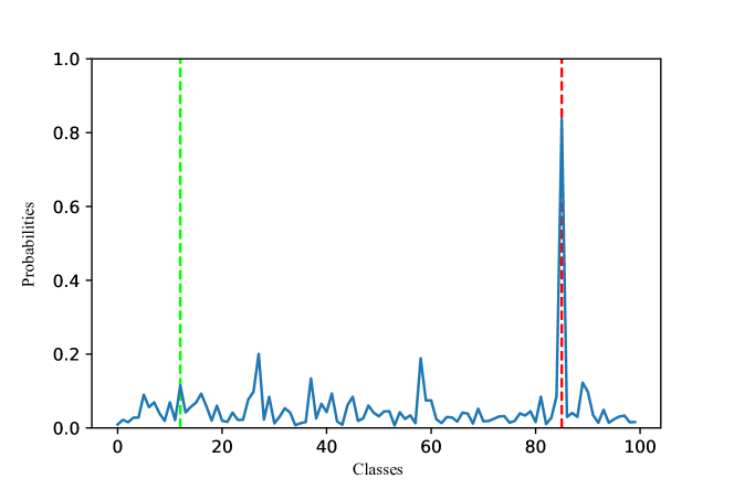
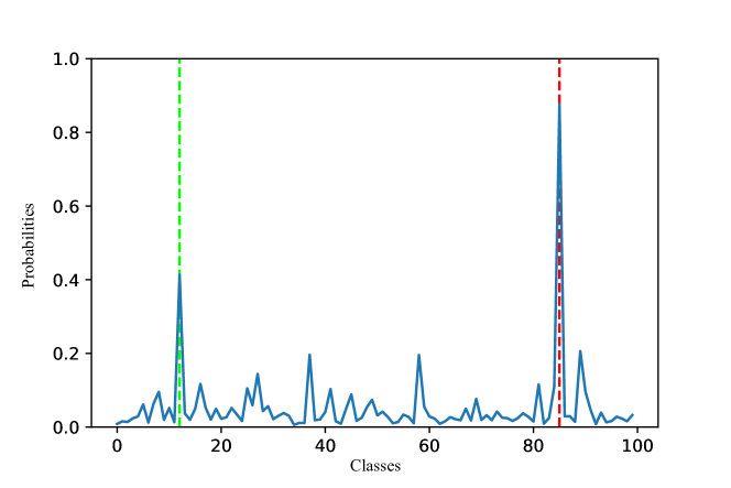
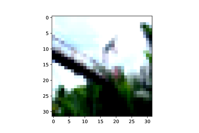
Visualization of correlation We visualize the aggregation of the teacher’s outputs and the student’s outputs. Fig. 2(a) and Fig. 2(b) are obtained by applying the maximum function to the outputs of each of the teacher (ResNet110) and one of the DCKD’s students (ResNet32) for all images of the tank class in CIFAR-100. To achieve a clearer distribution, we use , where is . Both distributions show peaks at their ground truth class and at other classes, which may correlate with the tank images. Although the teacher’s distribution and student’s distribution are similar in most classes, we observe another peak in the student’s distribution that does not appear in the teacher’s distribution. Fig. 3(a) shows the input data of the tank class that caused the peak for the bridge class in Fig. 2(b). The right side of Fig. 3(b) shows the sample input data of the bridge class, and since Fig. 3(a) and Fig. 3(b) appear similar, the student has a peak in the bridge class. The teacher model is well trained because it does not mistake tanks and bridges, but the well-trained teacher limits students from learning the correlation that reveals that tanks and bridges have similar features. These correlations, which the teacher is trained to disregard, can be important for students who seek to obtain as much information as possible.

| Teacher (Accuracy, %) DCKD Net1 DCKD Net2 DCKD Net3 | WRN-16-2 (76.85) (76.62) (76.52) | ResNet20 (73.09) (72.81) (72.61) | ResNet32 (75.33) (75.10) (74.87) | VGG8 (74.90) (74.76) (74.58) | MobileNetV2 (71.02) (70.78) (70.67) | ShuffleNetV1 (77.89) (77.41) (77.25) | ShuffleNetV2 (77.60) (77.49) (77.26) |
| Student Network (Accuracy, %) | WRN-16-2 (73.32) | ResNet20 (69.28) | ResNet32 (71.50) | VGG8 (70.92) | MobileNetV2 (65.23) | ShuffleNetV1 (71.34) | ShuffleNetV2 (73.89) |
| Method | Accuracy (std.) | ||||||
| eDCKD Net1 | 77.19 (0.08) | 72.70 (0.03) | 75.54 (0.03) | 75.26 (0.23) | 71.86 (0.16) | 77.51 (0.04) | 77.37 (0.06) |
| eDCKD Net2 | 77.05 (0.01) | 72.59 (0.04) | 75.33 (0.11) | 75.09 (0.09) | 71.57 (0.33) | 77.28 (0.13) | 77.11 (0.16) |
| eDCKD Net3 | 76.90 (0.11) | 72.43 (0.10) | 75.24 (0.15) | 74.99 (0.09) | 71.50 (0.28) | 77.00 (0.06) | 76.93 (0.08) |
| Ensembled Student | 77.05 (0.13) | 72.61 (0.07) | 75.28 (0.25) | 75.27 (0.12) | 71.08 (0.24) | 77.87 (0.15) | 77.26 (0.22) |
Knowledge accumulation Our motivation is to capture the correlation information between classes that the teacher may overlook. We investigate the aggregation of knowledge that was collected from the teacher, and DCKD’s students. In previous knowledge distillation studies, entropy was employed as a standard metric to analyze the correlations between labels. However, since the entropy is a measure of the degree of clustering in a distribution, it is not an ideal metric to evaluate correlations between classes. For example, if there are two distributions of and , the entropy of is higher than the entropy of , but does not convey any correlation information such as that of .
Therefore, to better evaluate the correlation information, we propose an alternative metric that is referred to as the correlation number, which is defined as follows:
| (15) |
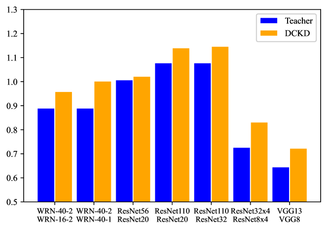
where is a distribution and is a class index. This metric counts the number of peaks in the distribution that are greater than ; therefore is 1 and is 2. Thus, the metric counts the significant correlations between classes. Fig. 4 shows that average correlation numbers of DCKD are higher than those of teachers. This suggests that DCKD’s students have additional information compared with their teachers and the knowledge collected from the students significantly enrich the knowledge of DCKD.
Further distillation We showed that DCKD’s students can be good teachers because they have a wealth of information on the correlations between classes. Therefore, we disseminate this accumulated knowledge from students with DCKD to the next generation of students via additional distillation, and we call this enhanced DCKD (eDCKD). Instead of using DCKD’s teacher, we utilize the students of DCKD as teachers for eDCKD’s students. We define that of (4) is the ensembled output of the DCKD’s students to utilize the accumulated knowledge considering the correlations between classes. We train new student models of the eDCKD using (9) with a newly defined .
Tab. 8 shows that the performance of eDCKD is as good as that of DCKD although eDCKD’s students were not trained with teachers of DCKD. Moreover, some experiments show that eDCKD’s students perform better than their teachers, DCKD’s students. Thus, DCKD’s students have various correlational information, and the additional knowledge is helpful for teaching eDCKD’s students.
In Tab. 8, an ensembled student model is a single student model trained with the knowledge of three DCKD students. Since we pursued a single compression model, we created an ensembled student model that combined the rich knowledge of multistudents into one. The performances of ensembled students are improved over all the pretrained student models and some DCKD’s students.
5 Conclusion
We have proposed a series of new methods for knowledge distillation based on the notion that the teacher model may not have all of the knowledge that students need. To collect and transfer rich knowledge that the teacher does not provide, we utilized multistudent models and applied the reverse KL divergence to increase the entropy, which soften the output distributions. We applied our method to a variety of deep neural networks to observe a collection of knowledge that takes into account the relation between classes. Our simple, effective method for collecting and transferring knowledge has improved student models with a state-of-the-art performance across a variety of architectures and datasets.
References
- [1] Cristian Buciluǎ, Rich Caruana, and Alexandru Niculescu-Mizil. Model compression. In Proceedings of the 12th ACM SIGKDD International Conference on Knowledge Discovery and Data Mining. ACM, 2006.
- [2] Defang Chen, Jian-Ping Mei, Can Wang, Yan Feng, and Chun Chen. Online knowledge distillation with diverse peers. In Proceedings of the AAAI Conference on Artificial Intelligence, 2020.
- [3] Jia Deng, Wei Dong, Richard Socher, Li-Jia Li, Kai Li, and Li Fei-Fei. Imagenet: A large-scale hierarchical image database. In Proceedings of the IEEE Conference on Computer Vision and Pattern Recognition (CVPR), 2009.
- [4] Abhimanyu Dubey, Otkrist Gupta, Ramesh Raskar, and Nikhil Naik. Maximum-entropy fine-grained classification, 2018.
- [5] Qiushan Guo, Xinjiang Wang, Yichao Wu, Zhipeng Yu, Ding Liang, Xiaolin Hu, and Ping Luo. Online knowledge distillation via collaborative learning. In Proceedings of the IEEE Conference on Computer Vision and Pattern Recognition (CVPR), 2020.
- [6] Kaiming He, Xiangyu Zhang, Shaoqing Ren, and Jian Sun. Deep residual learning for image recognition. In Proceedings of the IEEE Conference on Computer Vision and Pattern Recognition (CVPR), 2016.
- [7] Byeongho Heo, Jeesoo Kim, Sangdoo Yun, Hyojin Park, Nojun Kwak, and Jin Young Choi. A comprehensive overhaul of feature distillation, 2019.
- [8] Geoffrey Hinton, Oriol Vinyals, and Jeff Dean. Distilling the Knowledge in a Neural Network. arXiv preprint arXiv:1503.02531, 2015.
- [9] Andrew G. Howard, Menglong Zhu, Bo Chen, Dmitry Kalenichenko, Weijun Wang, Tobias Weyand, Marco Andreetto, and Hartwig Adam. MobileNets: Efficient Convolutional Neural Networks for Mobile Vision Applications. In Computer Vision and Pattern Recognition (CVPR), 2009.
- [10] Jangho Kim, Seong Uk Park, and Nojun Kwak. Paraphrasing complex network: Network compression via factor transfer. In Advances in Neural Information Processing Systems (NeurIPS), 2018.
- [11] Alex Krizhevsky. Learning multiple layers of features from tiny images. University of Toronto, 05 2012.
- [12] Xu Lan, Xiatian Zhu, and Shaogang Gong. Knowledge distillation by on-the-fly native ensemble. In Advances in Neural Information Processing Systems (NeurIPS), 2018.
- [13] Ilya Loshchilov and Frank Hutter. SGDR: Stochastic gradient descent with warm restarts. In International Conference on Learning Representations (ICLR), 2017.
- [14] Wonpyo Park, Dongju Kim, Yan Lu, and Minsu Cho. Relational knowledge distillation. In Proceedings of the IEEE Conference on Computer Vision and Pattern Recognition (CVPR), 2019.
- [15] Baoyun Peng, Xiao Jin, Dongsheng Li, Shunfeng Zhou, Yichao Wu, Jiaheng Liu, Zhaoning Zhang, and Yu Liu. Correlation congruence for knowledge distillation. In Proceedings of the IEEE International Conference on Computer Vision (ICCV), 2019.
- [16] Hengshuang Zhao Pengguang Chen, Shu Liu and Jiaya Jia. Distilling knowledge via knowledge review. In IEEE Conference on Computer Vision and Pattern Recognition (CVPR), 2021.
- [17] Gabriel Pereyra, George Tucker, Jan Chorowski, Łukasz Kaiser, and Geoffrey Hinton. Regularizing neural networks by penalizing confident output distributions. In International Conference on Learning Representations (ICLR), 2017.
- [18] Adriana Romero, Nicolas Ballas, Samira Ebrahimi Kahou, Antoine Chassang, Carlo Gatta, and Yoshua Bengio. FitNets: Hints for thin deep nets. In International Conference on Learning Representations (ICLR), 2015.
- [19] Karen Simonyan and Andrew Zisserman. Very deep convolutional networks for large-scale image recognition. In International Conference on Learning Representations (ICLR), 2015.
- [20] Sunil Thulasidasan, Gopinath Chennupati, Jeff Bilmes, Tanmoy Bhattacharya, and Sarah Michalak. On mixup training: Improved calibration and predictive uncertainty for deep neural networks, 2020.
- [21] Yonglong Tian, Dilip Krishnan, and Phillip Isola. Contrastive representation distillation. In International Conference on Learning Representations (ICLR), 2020.
- [22] Han Xiao, Kashif Rasul, and Roland Vollgraf. Fashion-MNIST: a Novel Image Dataset for Benchmarking Machine Learning Algorithms. arxiv preprint arXiv:1708.07747, 2017.
- [23] Sergey Zagoruyko and Nikos Komodakis. Wide Residual Networks. In British Machine Vision Conference (BMVC), 2016.
- [24] Sergey Zagoruyko and Nikos Komodakis. Paying more attention to attention: Improving the performance of convolutional neural networks via attention transfer. In International Conference on Learning Representations (ICLR), 2017.
- [25] Xiangyu Zhang, Xinyu Zhou, Mengxiao Lin, and Jian Sun. ShuffleNet: An Extremely Efficient Convolutional Neural Network for Mobile Devices. In Proceedings of the IEEE Conference on Computer Vision and Pattern Recognition (CVPR), 2018.
- [26] Ying Zhang, Tao Xiang, Timothy M. Hospedales, and Huchuan Lu. Deep Mutual Learning. In Proceedings of the IEEE Conference on Computer Vision and Pattern Recognition (CVPR), 2018.