A ZX-Calculus Approach to Concatenated Graph Codes

Abstract

Quantum Error-Correcting Codes (QECCs) are vital for ensuring the reliability of quantum computing and quantum communication systems. Among QECCs, stabilizer codes, particularly graph codes, have attracted considerable attention due to their unique properties and potential applications. Concatenated codes, which combine multiple layers of quantum codes, offer a powerful technique for achieving high levels of error correction with a relatively low resource overhead. In this paper, we examine the concatenation of graph codes using the powerful and versatile graphical language of ZX-calculus. We establish a correspondence between the encoding map and ZX-diagrams, and provide a simple proof of the equivalence between encoding maps in the Pauli $X$ basis and the graphic operation “generalized local complementation" (GLC) as previously demonstrated in [J. Math. Phys. 52, 022201]. Our analysis reveals that the resulting concatenated code remains a graph code only when the encoding qubits of the same inner code are not directly connected. When they are directly connected, additional Clifford operations are necessary to transform the concatenated code into a graph code, thus generalizing the results in [J. Math. Phys. 52, 022201]. We further explore concatenated graph codes in different bases, including the examination of holographic codes as concatenated graph codes. Our findings showcase the potential of ZX-calculus in advancing the field of quantum error correction.

I Introduction

Quantum Error-Correcting Codes (QECCs) play a crucial role in the advancement of quantum computing and quantum communication systems. Due to the inherently fragile nature of quantum information, it is highly susceptible to errors arising from environmental noise, imperfect quantum gates, and measurement inaccuracies. These errors can lead to significant losses in computational accuracy and jeopardize the overall performance of quantum systems. To counteract these issues, QECCs have been developed to detect and correct errors without disturbing the delicate quantum states, thus safeguarding the integrity of quantum information and enabling the realization of fault-tolerant quantum computing Nielsen and Chuang (2002).

Stabilizer codes are prominent families of QECCs that have garnered considerable attention due to their unique properties and potential applications. Stabilizer codes are a generalization of additive classical codes to the quantum domain. They are characterized by a set of stabilizer operators, which preserve the encoded quantum state and provide a framework for efficiently detecting and correcting errors Gottesman (1997); Calderbank et al. (1998). Graph codes, a subclass of stabilizer codes, utilize graph states to represent codewords, where each vertex corresponds to a qubit, and edges represent entangling operations Briegel and Raussendorf (2001); Raussendorf and Briegel (2001); Hein et al. (2006); Schlingemann (2001); Schlingemann and Werner (2001); Markus Grassl (2002). The graph structure provides an intuitive way of visualizing the quantum state and its interactions, making these codes particularly appealing for constructing quantum codes with desirable error-correcting capabilities Cross et al. (2009); Chuang et al. (2009); Chen et al. (2008). Additionally, every graph code is local Clifford equivalent to a stabilizer code, which means that they can be transformed into each other through local Clifford operations Van den Nest et al. (2004); Dehaene and De Moor (2003); Hostens et al. (2005). In general a graph code can be represented by an encoding circuit as shown in FIG. 1.

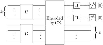
Figure 1: Encoding circuit for graph code: $k$ qubits are encoded into $n$ qubits; the $k$ qubits are input in the computational basis, followed by some $k$-qubit unitary $U$ that is a change of basis; $G$ is the encoding circuit for the corresponding graph state of the graph code; “Encoded by CZ” encodes the $k$ qubits into $n$-qubit graph code by some controlled-Z (CZ gates).

Concatenated quantum codes provide an important avenue for achieving high levels of error correction in quantum systems. By combining multiple layers of quantum codes, concatenated codes can achieve exponential improvements in error-correction performance with only a polynomial increase in resource overhead. This powerful technique enhances the resilience of quantum information against errors and is essential for the development of large-scale, fault-tolerant quantum computers Knill and Laflamme (1996); Knill et al. (1996, 1998); Zalka (1996); Aharonov and Ben-Or (1997). Furthermore, the versatility of concatenated codes allows for the integration of various types of QECCs, such as stabilizer codes and graph codes, leading to novel hybrid constructions that can leverage the advantages of each constituent code to optimize error-correcting capabilities Grassl et al. (2009, 2009). Encoding circuit for a concatenated code is illustrated in FIG. 2.

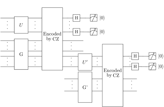
Figure 2: Encoding circuit for concatenated code: some qubits of the outer code (first layer of encoding on the left) are encoded into a inner code (second layer of encoding on the right), which is a graph code associated with graph $G^{\prime}$, with the Clifford operation $U^{\prime}$ that changes the basis of the encoded outer code qubits.

In Beigi et al. (2011), a graphical method was developed for concatenating graph codes. The main results of  Beigi et al. (2011) can be summarized as follows:

• For connected codes, the basis change map $U^{\prime}$ given by applying Hadamard $H$ to each encoding qubit of the inner code (i.e. encoding in the Pauli $X$ basis) is equivalent to a graphical operation known as “generalized local complementation" (GLC).

• When a GLC is applied to every encoding qubit of the inner code, the resulting concatenated code remains a graph code.

The primary advantage of this method lies in the ability to analyze code concatenation through a purely graphical approach. However, several questions remain unresolved, including:

• While the resulting concatenated code remains a graph code and can be obtained from the graphical operation GLC, the proof can only be provided using an algebraic method.

• The graphical method cannot be employed to analyze concatenation in any other basis (i.e. other choices of $U^{\prime}$), as the resulting concatenated code is not a graph code. Instead, it is a stabilizer code that requires certain Clifford operations to be transformed into a graph code.

ZX-calculus is a powerful and versatile graphical language for reasoning about and manipulating quantum states, particularly within the context of graph codes Coecke and Duncan (2007); Duncan and Perdrix (2009); van de Wetering (2020). Rooted in category theory principles, ZX-calculus uses a compact set of rules and graphical elements called ZX-diagrams to represent and manipulate quantum operations and states. In the domain of graph codes, ZX-diagrams offer an intuitive and visually appealing means of illustrating the underlying graph structure, where vertices represent qubits and edges indicate entangling operations. Applying the rules of ZX-calculus enables efficient transformations and simplifications of ZX-diagrams, which can assist in the analysis, optimization, and synthesis of graph codes. This graphical approach not only facilitates understanding complex quantum operations but also promotes the development of innovative error-correcting codes by exploring the rich combinatorial structures of graphs. Consequently, the integration of ZX-calculus and graph codes shows immense potential for advancing quantum error correction, ultimately leading to more efficient and robust quantum computing and communication systems.

The adaptability and flexibility of ZX-diagrams in handling stabilizer states and graph states suggest that they could be an effective tool for analyzing graph code concatenation. In this work, we apply ZX-calculus to examine the concatenation of graph codes. By establishing a correspondence between the encoding map and ZX-diagrams, we offer a straightforward proof of I1 using ZX-rules, providing a purely graphical method to address Q1. Upon further investigation, we find that I2 does not always hold; it is only valid when the encoding qubits of the inner code are not directly connected. When the encoding qubits are directly connected, additional Clifford operations are needed to transform the resulting concatenated code into a graph code. We then expand our analysis by utilizing ZX-diagrams to study concatenated graph codes for different $U$s (as answers for Q2), including the examination of holographic codes as concatenated graph codes. This approach illustrates the potential of ZX-calculus in driving the field of quantum error correction and enabling more efficient and resilient quantum computing and communication systems.

II Preliminaries

In this section, we present an overview of the preliminary concepts related to graph states, graph codes, and ZX-calculus, which will serve as the foundation for the subsequent parts of the paper.

II.1 Graph states and graph codes

Qubits are two-level quantum systems represented by the basis $|0\rangle,|1\rangle$. The Pauli matrices $X$ and $Z$ are defined as $X|0\rangle=|1\rangle,X|1\rangle=|0\rangle,$ and $Z|0\rangle=|0\rangle,Z|1\rangle=-|1\rangle.$ The Pauli group, generated by the Pauli matrices $X$ and $Z$, consists of all operators of the form $\pm X^{\mathbf{a}}Z^{\mathbf{b}}$, where $\mathbf{a},\mathbf{b}\in\{0,1\}^{n}$. We can represent these operators by the 2-length vector $(\mathbf{a}|\mathbf{b})$. Two Pauli operators commute if their corresponding vectors are orthogonal with respect to the symplectic inner product: $(\mathbf{a}|\mathbf{b})*(\mathbf{a^{\prime}}|\mathbf{b^{\prime}})=\mathbf{a}\mathbf{b^{\prime}}-\mathbf{a^{\prime}}\mathbf{b}.$ Now, consider $k$ pairwise commuting Pauli matrices $g_{1},\dots,g_{k}$ that generate a group without non-trivial multiples of the identity. These can be diagonalized simultaneously, and their eigenvalues are $\pm 1$. Let $|\psi\rangle$ be the eigenvector of $g_{1},\dots,g_{k}$ with eigenvalues $1$. Then, for each $i$, we have $g_{i}|\psi\rangle=|\psi\rangle$. $|\psi\rangle$ is the stabilizer state corresponding to the stabilizer group generated by $g_{1},\dots,g_{k}$.

The Clifford group is the normalizer of the Pauli group and is generated by the Hadamard gate, phase gate, and controlled-NOT gate. Clifford operators are important because they transform stabilizer states into stabilizer states. If $|\psi\rangle$ is a stabilizer state with stabilizer group $\mathcal{S}$ and $L$ is a Clifford operator, then $L|\psi\rangle$ is also a stabilizer state. Two stabilizer states are called “local Clifford equivalent” if they can be transformed into each other using local Clifford operators. Local Clifford operators preserve the entanglement of the states.

For the encoding circuits for graph codes, we need only two Clifford operators. First is the Hadamard gate $H|{r}\rangle=\frac{1}{\sqrt{2}}(|0\rangle+(-1)^{r}|1\rangle).$ Notice that $H=H^{\dagger}$, $HXH=Z$ and $HZH=X$. Hence, $H$ is in the Clifford group. The next operator is a two-qubit gate which is called controlled-$Z$ and is defined by $C_{z}|r\rangle|s\rangle=|r\rangle Z^{r}|s\rangle=(-1)^{rs}|r\rangle|s\rangle.$ Notice that $C_{z}=C_{z}^{\dagger}$, we have

$$C_{z}(X\otimes I)C_{z} = X\otimes Z,$$

$$C_{z}(I\otimes X)C_{z} = Z\otimes X,$$

$$C_{z}(Z\otimes I)C_{z} = Z\otimes I,$$

$$C_{z}(I\otimes Z)C_{z} = I\otimes Z,$$

and thus by definition $C_{z}$ is in the Clifford group.

Graph states are a special type of stabilizer states that can be represented by a graph with an adjacency matrix $G$. They can be generated using Hadamard and controlled-$Z$ gates. Studying graph states helps us understand stabilizer states since any stabilizer state is local Clifford equivalent to a graph state. To create a graph state corresponding to a graph with adjacency matrix $G$, we prepare $n$ qubits in the state $|0\rangle$, apply the Hadamard gate to each, and then apply controlled-$Z$ gates on qubits $i$ and $j$ with phase factor $(-1)^{g_{ij}}$. If we have a graph state $|\psi\rangle_{\mathcal{G}}$ corresponding to a graph $\mathcal{G}$ with adjacency matrix $G$, and we measure the last qubit in the standard basis, the resulting state (without the measured qubit) is also a graph state. The new graph state corresponds to the original graph $\mathcal{G}$ with the last vertex removed.

A $[[n,k,d]]$ graph code encodes $k$ qubits into $n$ qubits using a graph state $|\psi\rangle_{\mathcal{G}}$. To encode a state like $H\otimes\cdots\otimes H|r_{1}\dots r_{k}\rangle$, we first find the classical codeword $\boldsymbol{\alpha}$ in the linear code $\mathcal{C}$, which is a subspace of $\mathbb{F}_{2}^{n}$. We can represent $\mathcal{C}$ by $k$ basis vectors $\boldsymbol{\alpha}_{1},\dots,\boldsymbol{\alpha}_{k}$. The state is then encoded into $Z^{r_{1}\boldsymbol{\alpha}_{1}+\cdots+r_{k}\boldsymbol{\alpha}_{k}}|\psi\rangle_{\mathcal{G}}$. The encoding circuit for a $[[n,k,d]]$ graph code can be given as in the procedure below.

Procedure 1.

Encoding circuit for a graph code, as demonstrated in FIG. 1.

1. Generate the graph state $|\psi\rangle_{\mathcal{G}}$ with the encoding circuit $G$.

2. Apply the gate $U$ to the first $k$ qubits that we want to encode.

3. For each pair of qubits: $q_{i}$ of the encoding qubits and the $j$-th qubit of $|\psi\rangle_{\mathcal{G}}$, apply a controlled-$Z$ gate with phase factor $\alpha_{ij}$, where $\alpha_{ij}$ is the $j$-th coordinate of the basis vector $\boldsymbol{\alpha}_{i}$.

4. Apply the Hadamard gate $H$ to the first $k$ qubits.

5. Measure the first $k$ qubits in the computational basis.

II.2 ZX-calculus

In this section, we present a brief introduction to the ZX-calculus, a graphical language and powerful mathematical framework for representing and reasoning about quantum circuits and linear maps between qubits. For a comprehensive understanding, see e.g. Ref. van de Wetering (2020). ZX-calculus provides a diagrammatic notation for quantum states and operations, making it an invaluable tool for the manipulation, optimization, and simplification of quantum circuits.

Quantum computations in ZX calculus are represented as ZX-diagrams, consisting of two types of nodes: Z nodes (or Z spiders) and X nodes (or X spiders). Nodes are connected by edges that represent quantum entanglement or linear maps between the nodes. The linear maps corresponding to Z and X spiders can be explicitly written in Dirac notation, as illustrated in FIG. 3.

Figure 3: Definition of Z spider and X spider. Z spiders are represented by white nodes and X spiders are represented by grey nodes within this paper.

Another crucial element in ZX-calculus is the Hadamard gate, which is often represented by a white square or dashed line for simplicity, as demonstrated in FIG. 4. We will also give the ZX-diagram of controlled-Z gate without proof.

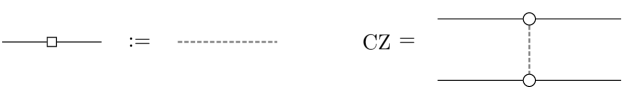
Figure 4: Representation of Hadamard gate and controlled-Z gate. The dashed line and white box both represent Hadamard gate.

In this paper, our primary focus is on Clifford ZX-diagrams, a special class of ZX-diagrams that represent Clifford circuits. Clifford circuits are quantum circuits composed exclusively of Clifford gates, which map Pauli operators to other Pauli operators (for example, Hadamard, CNOT, and Phase gates). Due to their efficient classical simulation algorithms and applications in quantum error correction, Clifford circuits play a significant role in quantum computing.

Clifford ZX-diagrams associate Z and X nodes with phases that are multiples of $\pi/2$. These diagrams can be simplified using a set of rewrite rules that preserve the semantics of the represented quantum computation. The complete set of rules for Clifford ZX-diagrams is shown in FIG. 5.

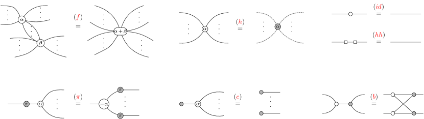
Figure 5: Basic rules for Clifford ZX-diagrams. These rules hold for all $\alpha,\beta\in[0,2\pi)$, and due to (${\color[rgb]{1,0,0}h}$) and (${\color[rgb]{1,0,0}hh}$) all rules also hold with the colours interchanged.

We will also frequently use two rules given in FIG. 6. By applying all these rules, we will construct rules for graph code concatenation.

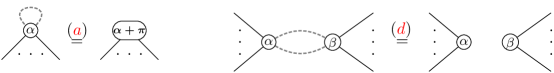
Figure 6: Two frequently used rules within this paper, as illustrated by Equations (83) and (94) in the work of van de Wetering (2020).

III From encoding circuit to ZX-diagrams

In this section we discuss encoding circuit (as given by Procedure 1) with ZX-diagrams. We start from mapping the encoding circuit as given in FIG. 1 into the form of a ZX-diagram.

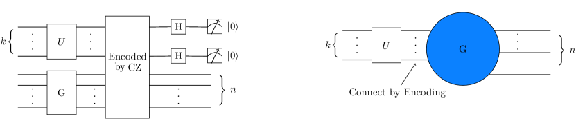
Figure 7: Encoding circuit of a graph code (left) as a ZX-digram (right).The encoder encodes $k$ qubits into $n$ qubits.

We have the following observation:

Observation 1.

As shown in FIG. 7, for any encoding circuit of the left, we can map it into into a ZX-graph as the right. Here $U$ is some Clifford operation and $G$ is a graph encoder for the left and a “graph state" as in ZX-calculus. The encoder encodes $k$ qubits into $n$ qubits.

Notice that this has some connections to Cao and Lackey (2022), but not used for the same purpose. To show that Observation 1 is valid, we translate the part of “encode by CZ" to ZX-diagram as shown in FIG. 8.

Figure 8: Proof of Observation 1: the mapping from encoding circuit to ZX-diagram, procedure goes from top left to bottom right, by first translating the “Encoded by CZ” and measurement part to a ZX-diagram, then apply the ZX-diagram rules.

We will give some concrete examples about how to translate encoding circuit into ZX-diagram.

Example 1.

Consider a [[3,1,1]] stabilizer code, its encoding circuit is shown in FIG.9. By Observation 1, we first connect qubit $1,2,3$ by graph and then encode $q_{0}$ with $1,2,3$ with $\mathrm{CZ}$.

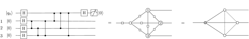
Figure 9: Figure of Example 1: Encoding circuit for [[3, 1, 1]] stabilizer code can be translated into ZX-diagram according to Observation 1.

Example 2.

Consider a graph code with three input and three output, as shown in FIG. 10.

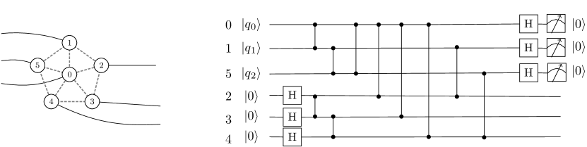
Figure 10: Figure of Example 2: A graph code with three input and three output. The ZX-diagram and corresponding encoding circuit.

In this case we have the $U$ given by

$$U=\mathrm{CZ}_{01}\mathrm{CZ}_{15}\mathrm{CZ}_{05}$$

Based on Observation 1, concatenated graph code by concatenating the encoding circuit (as illustrated in FIG.2) will corresponds to the connecting the ZX-graphs on the right. We demonstrate this with the following Example 3.

Example 3.

Concatenation of two five-qubit codes, as shown in FIG. 11. Here we first encode $A$ into a graph of $1,2,3,\alpha,\beta$, then we identify $\alpha$ with $\alpha^{\prime}$ and further encode $\alpha$ and $B$ into $4,5,6,\gamma^{\prime}$. The encoding circuits is given on the right. For the encoding of $\alpha$ and $B$ into $4,5,6,\gamma^{\prime}$, the corresponding $U^{\prime}$ is given by $\mathrm{CZ}_{B\alpha}$. Once can see the result is the same as if we first encode $B$ into $4,5,6,\alpha^{\prime},\gamma^{\prime}$, then we identify $\alpha$ with $\alpha^{\prime}$ and further encode $\alpha^{\prime}$ and $A$ into $1,2,3,\beta$.

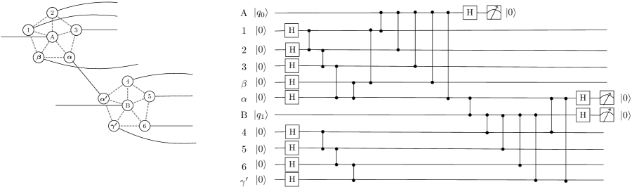
Figure 11: Figure of Example 3: ZX-diagram and encoding circuit for concatenation of two pentagon codes. The output qubit $\alpha$ of the outer code is concatenated with the input qubit $\alpha^{\prime}$ of the inner code.

It should be noted that, in general, concatenated graph codes do not qualify as graph codes. However, they are still stabilizer codes that are locally equivalent to graph codes under Clifford operations. In Beigi et al. (2011), it has been observed that when the encoding operation $U^{\prime}$ is the tensor product of Hadamard on each encoding qubit of the inner code (which is referred to as the case $U^{\prime}=H$ for simplicity), the resulting concatenated graph code still preserves the graph code property. This is achieved by employing a graphical operation known as "generalized local complementation" on each encoded qubit. The next section will provide a detailed examination of this particular case.

IV Generalized Local Complementation

The operation of “generalized local complementation" (GLC), as defined below, is a key concept in the construction of concatenated graph code as proposed in Beigi et al. (2011).

Definition (Generalized Local Complementation): Given a graph $\mathcal{G}$, let $N(i)$ denote the set of adjacent vertices of vertex $i$. Additionally, let $S$ be another subset of vertices. If $S=N(i)$, the GLC coincides with the definition of local complementation (LC). However, in this paper, $S$ is chosen to be disjoint from $N(i)$. A generalized local complementation on $i$ with respect to $S$ replaces the bipartite subgraph induced on $N(i)\cup S$ with its complement, as shown in FIG. 12.

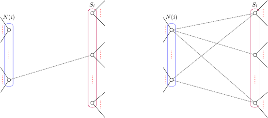
Figure 12: Generalized local complementation on $i$ with respect to a set $S_{i}$

In the context of encoding graphs for concatenated codes, we define $N(i)$ to be all the nodes adjacent to qubit $i$ in the outer graph. $S_{i}$ is defined as the set of nodes in the inner graph connected to $i$ via an encoding mapping. The gray node on the left in FIG. 13 represents the encoder of the inner graph.

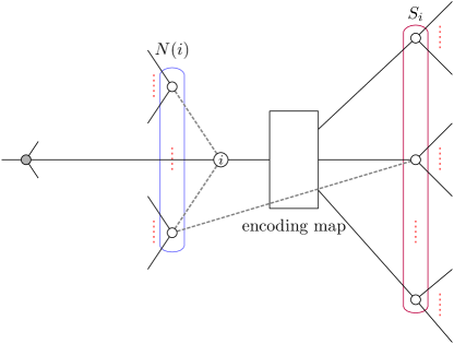
Figure 13: The encoding map for qubit $i$ is defined by the sets $N(i)$ and $S_{i}$. $N(i)$ is the set of all nodes adjacent to $i$ in the outer graph, while $S_{i}$ is the set of nodes in the inner graph that are connected to $i$ via an encoding mapping.

The significant finding of Beigi et al. (2011) is based on the following observation:

Observation 2.

GLC is equivalent to applying the $U^{\prime}=H$ concatenation encoding maps shown in FIG. 14.

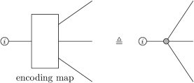
Figure 14: Concatenation encoding map with $U^{\prime}=H$.

The proof of this observation provided in Beigi et al. (2011) uses an algebraic method. In this paper, we present an alternative proof using ZX-diagrams, as depicted in FIG.15.

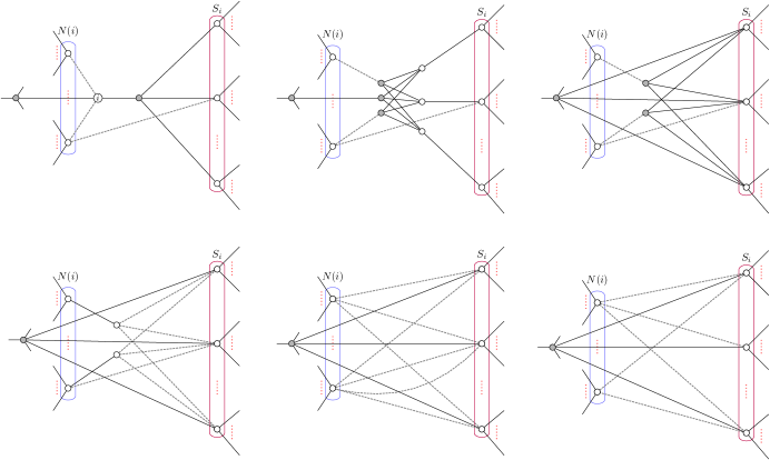
Figure 15: Proof of Observation 2: The equivalence between concatenated encoding with $U^{\prime}=H$ and the generalized local complementation rule.

The last equivalence in FIG.15 is derived using rule ($\color[rgb]{1,0,0}{d}$) in FIG.6. The encoders of the outer and inner graphs are merged to form a unified encoder.

Remark: GLC can be viewed as a special case of the variational pivot rule given in Eq. (103) of van de Wetering (2020), with $k=j=0$ and $N(u)\cap N(v)=\emptyset$, as depicted in FIG. 16.

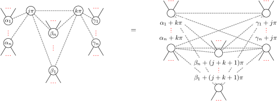
Figure 16: The variational pivot rule in Eq. (103) of van de Wetering (2020) with $k=j=0$ and $N(u)\cap N(v)=\emptyset$.

Applying the rule shown in FIG.16 also results in the equivalence between concatenated encoding with $U^{\prime}=H$ and generalized local complementation, as shown in FIG.17.

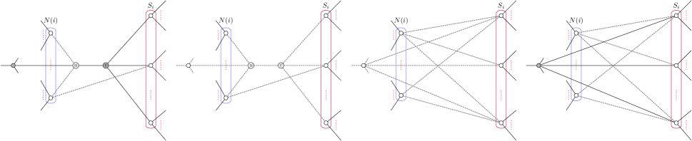
Figure 17: The equivalence between concatenated encoding with $U^{\prime}=H$ and generalized local complementation, derived from the variational pivot rule given in FIG. 16.

We illustrate these concepts through the following example:

Example 4.

Consider the concatenation of two encoders from Example 1. Starting from the top-left of FIG. 18, we sequentially apply the bialgebra rule ($\color[rgb]{1,0,0}{b}$), the Hadamard rule ($\color[rgb]{1,0,0}{h}$), and the fusing rule ($\color[rgb]{1,0,0}{f}$), which lead to the final graph code.

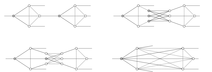
Figure 18: Figure for Example 4: Concatenation of two three-qubit graph codes with $U^{\prime}=H$. One of the output qubits of the outer code concatenates with the input qubit of the inner code. After simplification using ZX-diagrams, the resulting graph code is the same as applying GLC.

Additional examples (Example 9 and Example 10) are provided in the Appendix.

V Concatenation with $U^{\prime}=H$

This section explores the case where $U^{\prime}=H$, highlighting varying structures. It will focus on the scenario where multiple inner codes are present simultaneously.

The primary results of Beigi et al. (2011), namely I1 and I2, were summarized in Section I. In Section III, we demonstrated that I1 holds true using ZX-diagrams. However, upon further examination, it was revealed that I2 does not always hold in the context of the resulting concatenated codes. Specifically, I2 fails when qubits in the inner code correspond to multiple encoded qubits of the outer code, and these encoded qubits are directly connected.

V.1 Concatenation without loop

By the definition of "concatenation without loop", each qubit in the inner code should correspond to a unique encoded qubit in the outer code.

Observation 3.

When outer code and multiple inner codes concatenate without a loop, the resulting concatenated code is a graph code.

The proof of Observation 3 is given in FIG. 19.

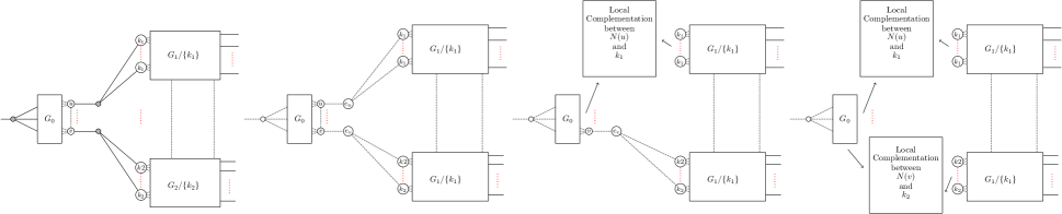
Figure 19: Proof of Observation 3: This figure depicts a Generalized Local Clifford (GLC) transformation for the general case where concatenation occurs without a loop. Here, $G_{0}$ is the outer code, while $G_{1}$ and $G_{2}$ are the inner codes. Nodes $u$ and $v$ are output qubits of the outer code. The sets $\{k_{1}\}$ and $\{k_{2}\}$ represent the qubits in the inner code that are connected to qubits $u$ and $v$ by a Hadamard encoder, respectively. This diagram exemplifies concatenation without a loop, as each qubit in the inner code corresponds to a unique encoded qubit in the outer code.

V.2 Loop concatenation without directly connected cooperative nodes

In loop concatenation, a node in the inner code may correspond to several encoded nodes in the outer code. For clarity, we define encoded nodes sharing a common encoding node in the inner codes as "cooperative nodes".

The variational pivot rule, as shown in FIG.16, is first applied to the case where two cooperative nodes are not directly connected, illustrated in FIG.20.

It is necessary for the encoded white node $v$ not to belong to the adjacent set $N(u)$ of another encoded white node $u$. This condition holds significance as the pair of cooperative nodes $(v,u)$ shares common encoding qubits in the inner code.

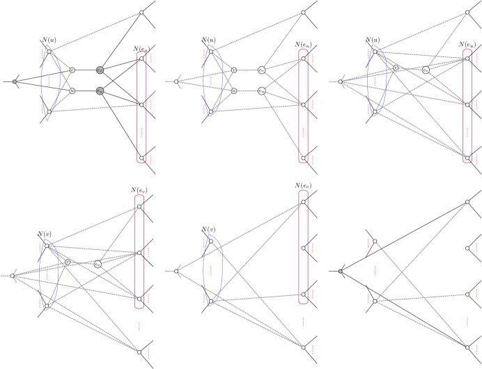
Figure 20: GLC for the case where cooperative nodes are not directly connected. As defined previously, $N(u)$ and $N(v)$ are the neighbors of $u$ and $v$ respectively, while $N(e_{u})$ and $N(e_{v})$ denote the neighbors of $e_{u}$ and $e_{v}$ respectively. The nodes $u$ and $v$ are identified as cooperative nodes because they are encoded to the top two nodes in $N(e_{u})$ simultaneously. The resulting concatenated code remains a graph code.

We now consider the general case where encoded white nodes sharing common encoding qubits are not directly connected.

Observation 4.

When all cooperative outer codes are not directly connected, the resulting concatenated code is a graph code.

The validity of Observation 4 can be shown by considering two arbitrary cooperative encoded nodes $u$ and $v$ connected in two inner graphs $G_{1}$ and $G_{2}$ through a Hadamard encoder. As shown in FIG. 21, where $e_{\mu}$ and $e_{\nu}$ denote the encoders of nodes $\mu$ and $\nu$ respectively, $j_{1}\in G_{1}$ and $j_{2}\in G_{2}$ denote the sets of vertices that are connected to both $e_{\mu}$ and $e_{\nu}$. $k_{1}$ denotes the set of vertices that are only connected to $e_{\mu}$, and $k_{2}$ denotes the set of vertices that are only connected to $e_{\nu}$. Without loss of generality, we can arrange all $k_{1}\in G_{1}$ and all $k_{2}\in G_{2}$ by redefining $G_{1}$ and $G_{2}$, as there is no limitation on the links between $G_{1}$ and $G_{2}$.

Our goal is to prove that the loop concatenated code remains a graph code, unless nodes $u$ and $v$ are directly connected.

To do so,we need to remove the nodes $u$ and $v$, as well as their corresponding encoders $e_{u}$ and $e_{v}$, from the graph. Then, we can apply the variational pivot rule in FIG.16. The procedure is illustrated in FIG. 21.

Figure 21: Proof of Observation 4: GLC for the general case in which cooperative qubits are not directly connected. Unlike in FIG.19, $u$ and $v$ are now considered cooperative nodes, as they are simultaneously encoded into $\{j_{1}\}$ and $\{j_{2}\}$, respectively. Notably, there is no edge between the cooperative nodes $u$ and $v$.

Firstly, we note that the subgraphs $G_{0}/{N(v)\cup N(u)}$, $G_{1}/{k_{1}\cup j_{1}}$, and $G_{2}/{k_{2}\cup j_{2}}$ are entirely irrelevant to the variational pivot process, and they will remain unchanged until the end.

Since $N(u)\cap N(e_{u})=\emptyset$, the variational pivot rule will be reduced to the local complementation (LC) operation between $N(u)$ and $k_{1}\cup j_{1}\cup j_{2}$. The output of the LC operation will be another graph state.

A crucial fact is that $v\notin N(u)$, which prevents node $v$ from connecting to nodes in $k_{1}\cup j_{1}\cup j_{2}$ after the first LC operation. This ensures that the $\pi$ phase factor does not occur in the next pivot operation. Otherwise, if $N(v)\cap N(e_{v})\in j_{1}\cup j_{2}$, all nodes in $j_{1}\cup j_{2}$ would receive a $\pi$ phase according to FIG. 16.

Once $v\notin N(u)$, $N(v)\cap N(e_{v})$ could only be $\emptyset$, so the next pivot rule would also reduce to LC operation, which output graph state. Thus we removed nodes $u$, $v$ and their corresponding encoders $e_{u}$ and $e_{v}$ and output a graph state.

We can apply the aforementioned procedure iteratively to eliminate two additional nonadjacent encoded white nodes. This property can be extended to $n$ nonadjacent encoded white nodes simultaneously, provided they are not directly connected. Therefore, if the encoded white nodes remain nonadjacent to one another, the resulting concatenated code can be transformed into a graph state through multiple local complementation operations.

We will also give a simple example here.

Example 5.

Loop concatenation without directly connected cooperative nodes. We deliberately construct such concatenation. There is no edge between cooperative nodes. of inner codes that are used for next level concatenation.

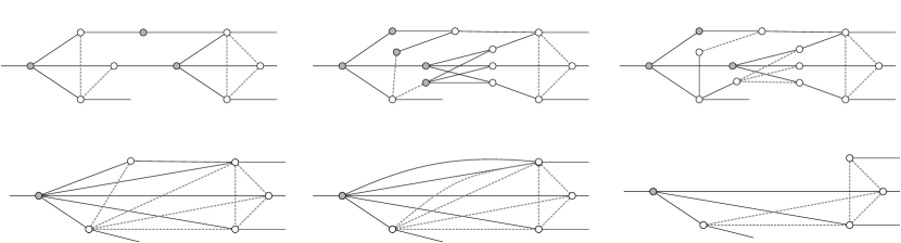
Figure 22: Figure for Example 5: Loop concatenation where cooperative nodes do not connect.

V.3 Loop concatenation with directly connected cooperative nodes

When direct edges exist between cooperative qubits, we refer to this as loop concatenation with directly connected cooperative nodes. In such scenarios, the following observation can be made:

Observation 5.

If two cooperative encoded nodes are directly connected, the resulting concatenated code is no longer a graph code, but is local Clifford equivalent to a graph code.

The validity of Observation 5 can be demonstrated through the graphical approach shown in FIG.23 and FIG.24. In these cases, the common nodes in the inner codes, encoded by both $u$ and $v$, end up with an additional $\pi$ phase factor. We provide an example to further elaborate on loop concatenation with directly connected cooperative nodes.

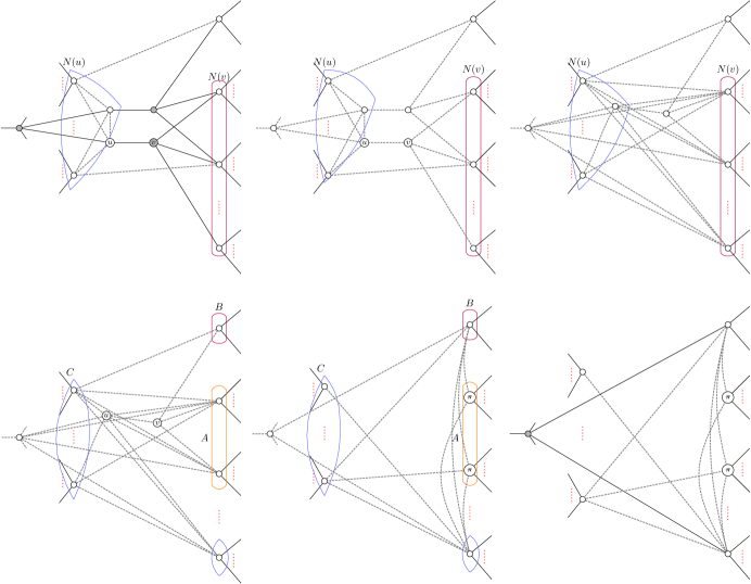
Figure 23: GLC for loop concatenation with cooperative nodes connected directly and steps of simplification. Compared with Fig 20, the cooperative nodes has a edge. The resulting concatenated code is local Clifford equivalent to a graph code.

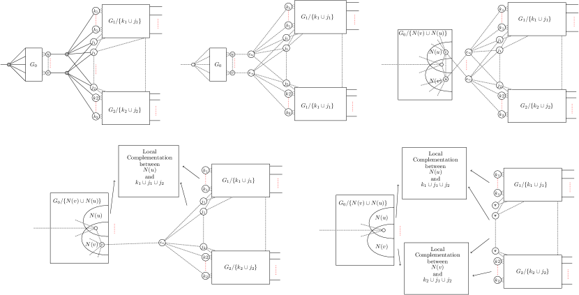
Figure 24: GLC for the general case when cooperative qubits are directly connected by a Hadamard edge. The notation here is identical to that in FIG. 21. Notably, a Hadamard edge exists between the cooperative nodes $u$ and $v$.

Example 6.

Loop concatenation with cooperative nodes connected directly. There exists direct edge between cooperative nodes. We keep using the [[3,1,1]] code as example for a clear comparison.

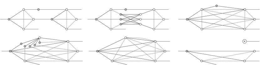
Figure 25: Figure for Example 6: Loop concatenation with directly connected cooperative nodes. Compared to Example 5 , the cooperative nodes are connected by an edge.

One more example can be found in Appendix (Example 11).

VI Concatenation with $U^{\prime}=I$

In this section, we focus on the ZX-diagram approach for concatenation in the scenario where $U^{\prime}=I$.

Consider $G_{1}$ and $G_{2}$ as two general graph states. For this discussion, we introduce the following notations:

• Node $i$: The node in $G_{1}$ that is connected to the encoder and $G_{2}$.

• $N(i)$: The set of neighbors of node $i$ in $G_{1}$.

• Node $j$: The node in $G_{2}$ that is selected for the application of the Hadamard rule ($\color[rgb]{1,0,0}{h}$).

• $S_{i}/j$: The set of neighbors nodes of node $i$ in $G_{2}$, excluding node $j$.

• $W(j)$: The set of neighbors nodes of node $j$ in $G_{2}$.

• $G_{2}/j$: The subgraph of $G_{2}$ without the node $j$.

We now detail the general procedure of concatenation for the case where $U^{\prime}=I$.

Procedure 2.

As illustrated in FIG. 26, the preliminary concatenation result of two general graphs $G_{1}$ and $G_{2}$ for $U^{\prime}=I$ after several steps of applying the Hadamard operation corresponds to the following:

• The encoder of $G_{1}$ is connected to $N(i)$, $j$, and $W(j)$.

• Node $j$ is connected to $N(i)$ and $S_{i}/j$ through the Hadamard edges.

• At this stage, $W(j)$ and $S_{i}/j$ are fully interconnected by the Hadamard edges.

• $G_{2}/j$ can be connected to $W(j)$ or $S_{i}/j$ via node $k$ if node $k$ is present in either $W(j)$ or $S_{i}/j$.

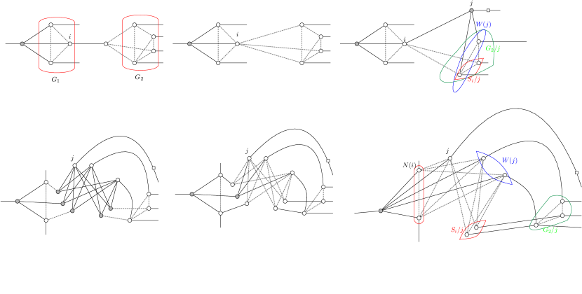
Figure 26: Illustration of Procedure 1 for concatenation where $U^{\prime}=I$. Node $i$ in $G_{1}$ is connected to both the encoder and $G_{2}$. The set $N(i)$ consists of its neighbors in $G_{1}$. The fuse rule ($\color[rgb]{1,0,0}f$) is then applied to node $i$. Subsequently, we select node $j$ and apply the Hadamard rule ($\color[rgb]{1,0,0}h$) to it. This allows us to define the following sets: $N(i)$, the set of node $i$’s neighbors in $G_{1}$; $S_{i}/j$, the set of node $i$’s neighbors in $G_{2}$, excluding node $j$; $W(j)$, the set of node $j$’s neighbors in $G_{2}$; and $G_{2}/j$, the subgraph of $G_{2}$ without node $j$. After applying the bi-algebra rule ($\color[rgb]{1,0,0}b$) and simplifying, we obtain the final figure, which will be further simplified in Procedure 2.

Next, we proceed to merge the identical nodes in $G_{2}/j$, $W(j)$, and $S_{i}/j$:

• For each node $k\in G_{2}/j$, if node $k$ is present in both $W(j)$ and $S_{i}/j$, then we add a $\pi$ phase to $k$. If not, it remains unchanged.

• For each edge $(k,l)\in G_{2}/j$, if any of the following conditions are met, edge $(k,l)$ remains unchanged:

  • Both $k$ and $l$ are present in $W(j)$ and $S_{i}/j$.

  • Neither $k$ nor $l$ are present in $W(j)$ or $S_{i}/j$.

  • $k$ is not present in either $W(j)$ or $S_{i}/j$.

  • $l$ is not present in either $W(j)$ or $S_{i}/j$.

  If none of the conditions are met, we remove edge $(k,l)$.

• All edges between $W(j)$ and $S_{i}/j$ are removed.

• Each node $k\in G_{2}/j$ is merged with the same node in $W(j)$ or $S_{i}/j$, eliminating any self-edges. Note that no self-edges would be found as step 3 eliminates all potential self-edges and step 1 adjusts for the phase.

Now, let’s delve into an example.

Example 7.

We consider a concatenation with $U^{\prime}=I$. The resulting graph is not a graph code. However, we can transform it into a graph code by pushing one Hadamard to the right. The procedure is illustrated in FIG. 27.

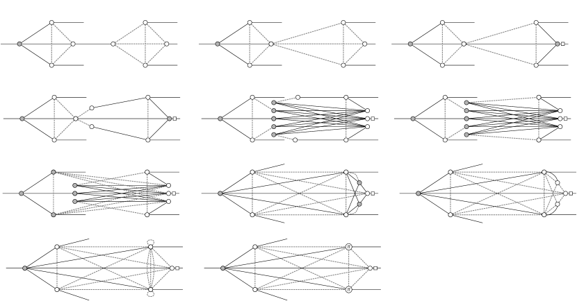
Figure 27: Figure for Example 7: Concatenation of [[3,1,1]] stabilizer code with $U^{\prime}=I$. The resulting code is local Clifford equivalent to the graph code in Fig.18.

An additional example can be found in Appendix (Example 12).

VII Holographic code as a concatenated code: concatenation with entangling $U$

Holographic codes are a class of quantum error-correcting codes that draw inspiration from the AdS/CFT holographic duality in theoretical physics Pastawski et al. (2015); Almheiri et al. (2015). These codes use encoding isometries to model the radial time evolution in Anti-de Sitter (AdS) space, mapping logical qudits in the bulk of AdS to physical qudits on the boundary of the corresponding Conformal Field Theory (CFT). Typically represented by tensor networks associated with a tiling of hyperbolic space, holographic codes protect against erasure errors on the boundary. The error-correction properties of these codes are often characterized in terms of which logical operators can be reconstructed after erasures. Specifically, bulk operators outside the entanglement wedges of the erased boundary operators can be reconstructed using the remaining boundary operators.

In Munné et al. (2022), holographic codes are examined from the perspective of stabilizer codes and graph codes. In this work, we will utilize the ZX-calculus approach to demonstrate that holographic codes can be viewed as concatenated graph codes. We will use the example from Munné et al. (2022), where $4$ bulk qubits are encoded to $12$ boundary qubits, and we will apply the following concatenation step:

• Encoding qubit $A$ into a five-qubit graph.

• Encoding qubit $\alpha$ along with qubit $B$, into qubits $4,5,6$, and $\gamma^{\prime}$ using some unitary transformation (the encoding circuit is demonstrated in Example 3).

• Encoding qubit $\gamma^{\prime}$ along with qubit $C$, into qubits $7,8,9$, and $\delta$ using some unitary transformation.

• Encoding qubits $\delta$, $\beta$ along with qubit $C$, into qubits $10,11,12$, using some unitary transformation, resulting in a fully encoded holographic code.

We illustrate this procedure in FIG. 29 with $U^{\prime}=I$. We start from the top left concatenated code and obtain the bottom right ZX-diagram that is local Clifford equivalent to a graph code.

Upon obtaining the encoding ZX diagram, we can further extract the logical state and its corresponding graph representation. The logical state $|G_{000}^{\text{opt}}\rangle$ of the encoding circuit, as shown in FIG. 28, is found to be local Clifford equivalent to the result obtained in Ref. Munné et al. (2022).

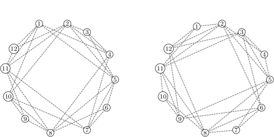
Figure 28: $|G_{000}^{\text{opt}}\rangle$ of holographic code. The left one is constructed by code concatenation with ZX-diagram and the right one is given in Munné et al. (2022). These two graphs are local Clifford equivalent, meaning they can be transformed into each other by local complementation.

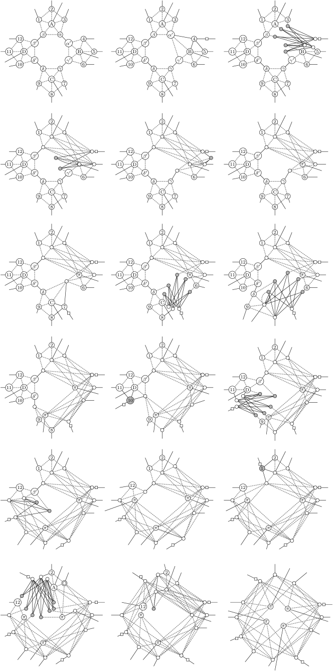
Figure 29: Holographic code as a concatenated graph code. It encodes 4 qubits ($ABCD$) into 12 qubits ($1-12$). We start from the top left figure, and subsequently remove qubit labels in later figures for simplicity. The result is the bottom right figure, where nodes with $\pi$ phase are input qubits.

VIII Conclusion and discussion

In this paper, we have successfully employed ZX-calculus as a graphical language to analyze the concatenation of graph codes. We have established a correspondence between the encoding map and ZX-diagrams and utilized the ZX-rules to provide a purely graphical proof of I1, addressing Q1. Our findings have revealed that I2 does not always hold, as it depends on the connectivity of the encoding qubits of the inner code. Furthermore, we have expanded our study by examining concatenated graph codes for different values of $U$, including holographic codes, offering insights into Q2.

The results presented in this work demonstrate the power and potential of ZX-calculus in the realm of quantum error correction. By providing a visually intuitive and algebraically rigorous framework for the analysis of graph code concatenation, we have laid the groundwork for further advancements in the design and optimization of error-correcting codes for quantum computing and communication systems.

Our study also suggests several avenues for future research. One possible direction is the generalization of our approach to the concatenation of stabilizer codes, not just concatenated graph codes. As an example, Shor’s code can be viewed as an concatenated code.

Example 8.

Shor’s code can be given by concatenation. However it is not in the form a graph code. It is indeed local Clifford (LC) equivalent to the graph code right figure below.

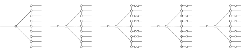
Figure 30: ZX-diagram:Shor’s code as a concatenated graph code.

By extending the methods developed in this paper, we may uncover new insights into the structure and properties of concatenated stabilizer codes, opening up new possibilities for error correction in a broader range of quantum systems.

Another promising area for future work is the investigation of symmetry in concatenated codes. It turns out, the concatenated graph code maintains some symmetry of the inner and outer code, as shown in various examples in this paper. A deeper understanding of the symmetries present in these codes could potentially lead to the development of more efficient error detection and correction procedures. Additionally, the exploration of symmetries may reveal connections between seemingly distinct codes, further enriching our understanding of the space of quantum error-correcting codes.

In conclusion, the application of ZX-calculus to the analysis of concatenated graph codes has not only yielded important insights into the structure and properties of these codes but has also paved the way for further research in the field of quantum error correction. By continuing to explore the rich combinatorial structures of graph codes and their concatenation, we can contribute to the development of more efficient and robust quantum computing.

Appendix: Additional Examples

In this appendix, we delve deeper into several examples to further illustrate the process of concatenation in different scenarios.

Example 9.

Here, we examine the concatenation of two five-qubit codes with $U^{\prime}=H$ as shown in Figure 31.

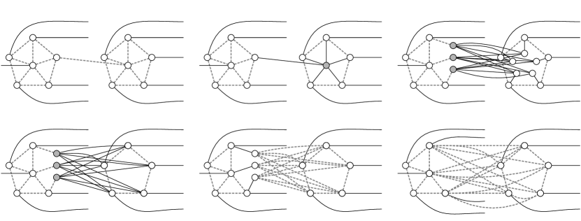
Figure 31: Concatenation of two five-qubit code. Notice that only one qubit of the outer code is encoded into an inner five-qubit code. One can use a similar procedure to encode all five qubits of the outer code, which will result in FIG.9 of  Beigi et al. (2011).

Example 10.

Let’s consider the concatenation of the Steane code with $U^{\prime}=H$ as illustrated in Figure 32.

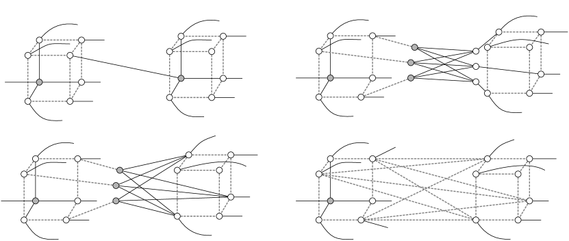
Figure 32: Concatenation of Steane code. Notice that only one qubit of the outer code is encoded into an inner Steane code. One can use a similar procedure to encode all seven qubits of the outer code, which will result in FIG.10 of  Beigi et al. (2011).

Example 11.

In this example, we consider a unique case of loop concatenation where the cooperative nodes are directly connected, as depicted in Figure 33.

Figure 33: Loop concatenation with directly connected cooperative nodes.

Example 12.

Concatenation of two five-qubit code with $U^{\prime}=I$:

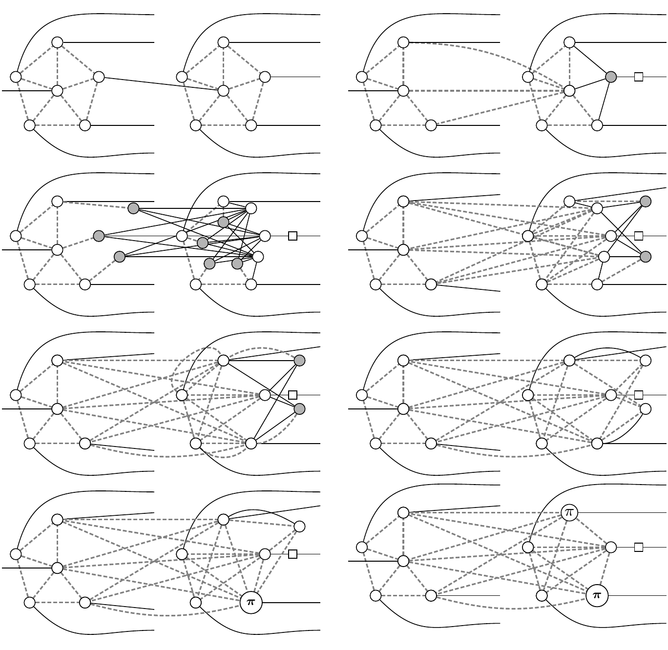
Figure 34: Concatenation of two five-qubit code with $U^{\prime}=I$.

References

- Nielsen and Chuang (2002) M. A. Nielsen and I. Chuang, Quantum computation and quantum information (2002).
- Gottesman (1997) D. Gottesman, Stabilizer codes and quantum error correction (California Institute of Technology, 1997).
- Calderbank et al. (1998) A. R. Calderbank, E. M. Rains, P. M. Shor, and N. J. Sloane, IEEE Transactions on Information Theory 44, 1369 (1998).
- Briegel and Raussendorf (2001) H. J. Briegel and R. Raussendorf, Physical Review Letters 86, 910 (2001).
- Raussendorf and Briegel (2001) R. Raussendorf and H. J. Briegel, Physical review letters 86, 5188 (2001).
- Hein et al. (2006) M. Hein, W. Dür, J. Eisert, R. Raussendorf, M. Nest, and H.-J. Briegel, arXiv preprint quant-ph/0602096 (2006).
- Schlingemann (2001) D. Schlingemann, arXiv preprint quant-ph/0111080 (2001).
- Schlingemann and Werner (2001) D. Schlingemann and R. F. Werner, Physical Review A 65, 012308 (2001).
- Markus Grassl (2002) M. R. Markus Grassl, Andreas Klappenecker, in Proceedings IEEE International Symposium on Information Theory, (IEEE, 2002), p. 45.
- Cross et al. (2009) A. Cross, G. Smith, J. Smolin, and B. Zeng, IEEE Transactions on Information Theory 1, 433 (2009).
- Chuang et al. (2009) I. Chuang, A. Cross, G. Smith, J. Smolin, and B. Zeng, Journal of Mathematical Physics 50, 042109 (2009).
- Chen et al. (2008) X. Chen, B. Zeng, and I. L. Chuang, Physical Review A 78, 062315 (2008).
- Van den Nest et al. (2004) M. Van den Nest, J. Dehaene, and B. De Moor, Physical Review A 69, 022316 (2004).
- Dehaene and De Moor (2003) J. Dehaene and B. De Moor, Physical Review A 68, 042318 (2003).
- Hostens et al. (2005) E. Hostens, J. Dehaene, and B. De Moor, Physical Review A 71, 042315 (2005).
- Knill and Laflamme (1996) E. Knill and R. Laflamme, arXiv preprint quant-ph/9608012 (1996).
- Knill et al. (1996) E. Knill, R. Laflamme, and W. Zurek, arXiv preprint quant-ph/9610011 (1996).
- Knill et al. (1998) E. Knill, R. Laflamme, and W. H. Zurek, Proceedings of the Royal Society of London. Series A: Mathematical, Physical and Engineering Sciences 454, 365 (1998).
- Zalka (1996) C. Zalka, arXiv preprint quant-ph/9612028 (1996).
- Aharonov and Ben-Or (1997) D. Aharonov and M. Ben-Or, in Proceedings of the twenty-ninth annual ACM symposium on Theory of computing (1997), pp. 176–188.
- Grassl et al. (2009) M. Grassl, P. Shor, G. Smith, J. Smolin, and B. Zeng, Physical Review A 79, 050306 (2009).
- Beigi et al. (2011) S. Beigi, I. Chuang, M. Grassl, P. Shor, and B. Zeng, Journal of Mathematical Physics 52, 022201 (2011).
- Coecke and Duncan (2007) B. Coecke and R. Duncan, Preprint (2007).
- Duncan and Perdrix (2009) R. Duncan and S. Perdrix, in Conference on Computability in Europe (Springer, 2009), pp. 167–177.
- van de Wetering (2020) J. van de Wetering, arXiv preprint arXiv:2012.13966 (2020).
- Cao and Lackey (2022) C. Cao and B. Lackey, PRX Quantum 3, 020332 (2022).
- Pastawski et al. (2015) F. Pastawski, B. Yoshida, D. Harlow, and J. Preskill, Journal of High Energy Physics 2015, 1 (2015).
- Almheiri et al. (2015) A. Almheiri, X. Dong, and D. Harlow, Journal of High Energy Physics 2015, 1 (2015).
- Munné et al. (2022) G. A. Munné, V. Kasper, and F. Huber, arXiv preprint arXiv:2209.08954 (2022).