Extended dissipaton equation of motion for electronic open quantum systems:
Application to the Kondo impurity model

Abstract

In this paper, we present an extended dissipaton equation of motion for studying the dynamics of electronic impurity systems. Compared with the original theoretical formalism, the quadratic couplings are introduced into the Hamiltonian accounting for the interaction between the impurity and its surrounding environment. By exploiting the quadratic fermionic dissipaton algebra, the proposed extended dissipaton equation of motion offers a powerful tool for studying the dynamical behaviors of electronic impurity systems, particularly in situations where nonequilibrium and strongly correlated effects play significant roles. Numerical demonstrations are carried out to investigate the temperature dependence of the Kondo resonance in the Kondo impurity model.

I Introduction

Electronic impurity systems are important in a wide range of fields, including solid–state physics, materials science, quantum information, and so on. [1, 2, 3, 4, 5] The dynamics of these systems are particularly intriguing due to the strong coupling between the impurity and its surrounding environment. [6, 7, 8, 9, 10, 11, 12, 13, 14] The study of electronic impurity systems is crucial for understanding the behavior of materials and quantum devices, and has practical implications for designing new technologies. [15, 16, 17, 18, 19, 20, 21, 22]

One of the main challenges in studying electronic impurity systems is accurately modeling their interactions with the environment. The Anderson and Kondo impurity models are widely used for describing the impurity system within the fermionic environments. The Anderson model describes a local quantum impurity coupled to non-interacting conduction electrons in a metal, where the impurity system is represented by a single electronic level interacting with a continuum of reservoir states. The system–bath coupling is in the linear form with respect to the creation and annihilation operators of the impurity and bath states, $H_{\mbox{\tiny SB}}\sim\sum_{ks}(t_{ks}\hat{d}_{ks}^{\dagger}\hat{a}_{s}+{\rm h.c.})$. The other model, the Kondo impurity model, is famous for successfully predicting the emergence of a many–body state at low temperatures, known as the Kondo resonance, which is featured as a sharp peak in the vicinity of the Fermi level of the metal electrons. The Kondo impurity model is analogous to the Anderson impurity model, describing an impurity spin coupled to conduction electrons in a metal. But the electron–electron interactions take a Heisenberg coupling form, $H_{\mbox{\tiny SB}}\sim J{\bm{S}}_{\rm imp}\cdot{\bm{S}}_{{\mbox{\tiny B}}}$, where $J$ is the exchange coupling constant between the impurity spin ${\bm{S}}_{\rm imp}$ and the conduction electrons total spin ${\bm{S}}_{{\mbox{\tiny B}}}$, and ${\bm{S}}_{{\mbox{\tiny B}}}$ is quadratic with respect to the reservoir creation and annihilation operators.

So far, various methods have targeted the equilibrium and dynamical properties of quantum impurities, such as the quantum Monte Carlo method, [23, 24] the numerical renormalization group method [25, 26, 27, 28, 29, 30] and its time–dependent extension, [31, 32] the time–dependent density matrix renormalization group method, [33, 34], and so on. The recent developments in methods include the time evolving density matrices using orthogonal polynomials algorithm (TEDOPA), [35, 36] the time-evolving matrix product operator (TEMPO) algorithm, [37, 38] the automated compression of environments (ACE) method, [39] the inchworm quantum Monte Carlo method, [40, 41, 42] the quantum quasi-Monte Carlo algorithm, [43] and the auxiliary master equation approach (AMEA). [44]

Especially, as a time–derivative equivalence to the Feynman–Vernon influence functional path,[45] the hierarchical equations of motion (HEOM) method has attracted increasing attention, with either bosonic [46, 47, 48, 49, 50, 51, 52, 53] or fermionic bath environment influence. [54, 55, 56] Earlier applications of the HEOM method have been mainly focused on the Anderson impurity model, because the method is developed on the basis of a linear system–bath coupling scenario. The extension to considering also the quadratic system–bath coupling form, which is the case for the Kondo impurity model, is yet to be developed. The Kondo impurity model has so far been dealt with by such as the renormalization group approach.[25, 57, 32]

Dissipaton equation of motion (DEOM),[58, 59] as a second quantization version of HEOM, is able to acquire the dynamics in the presence of nonlinear coupling in the bosonic scenarios. [60, 61] Its exactness has been numerically verified recently.[62] In this work, we propose the fermionic version of the extended DEOM (ext-DEOM) for the fermionic quadratic coupling between the system and bath. This addresses the challenge of DEOM to deal with the Kondo impurity model, where the quadratic couplings between the impurity and its environment are involved. This extension builds upon previously developed fermionic dissipaton algebra introduced for linear couplings and expands the capabilities to quadratic environment coupling scenarios.

The remainder of this paper is organized as follows: In Sec. II, we propose the ext-DEOM with a detailed derivation. In Sec. III, we demonstrate the temperature-dependent Kondo resonance in the Kondo impurity model. Finally, we summarize our paper in Sec. IV. Throughout this paper, we set $\hbar=1$ and $\beta=1/(k_{B}T)$, with $k_{B}$ being the Boltzmann constant and $T$ the temperature.

II Extended dissipaton equation of motion

II.1 Quadratic system–bath interactions

In this work, we consider an electronic system ($H_{{\mbox{\tiny S}}}$) in contact with a fermionic bath ($h_{{\mbox{\tiny B}}}$). While $H_{{\mbox{\tiny S}}}$ is arbitrary, the bath Hamiltonian $h_{{\mbox{\tiny B}}}$ is modeled as noninteracting electrons,

$$h_{{\mbox{\tiny B}}}=\sum_{ks}\epsilon_{ks}\hat{d}^{+}_{ks}\hat{d}_{ks}^{-},$$ (1)

where $k$ and $s=\uparrow,\downarrow$ label a single–electron spin–orbital state. The system and bath couple with each other via the quadratic interaction,

$$H_{\mbox{\tiny SB}}=\frac{1}{2}\sum_{\sigma us}\sum_{\sigma^{\prime}vs^{\prime}}\hat{q}^{\bar{\sigma}\bar{\sigma}^{\prime}}_{us,vs^{\prime}}\hat{\Phi}^{\sigma}_{us}\hat{\Phi}^{\sigma^{\prime}}_{vs^{\prime}}.$$ (2)

Here, $\sigma\in\{+,-\}$ and the hybridizing bath operators read

$$\hat{\Phi}^{+}_{us}\equiv\sum_{k}c_{kus}{\color[rgb]{0,0,0}\hat{d}^{+}_{ks}}\equiv(\hat{\Phi}^{-}_{us})^{\dagger}.$$ (3)

$\{\hat{q}^{\sigma\sigma^{\prime}}_{us,vs^{\prime}}\}$ are the system subspace operators, generally quadratic in terms of the system creation/annihilation operators $\{\hat{a}_{us}^{\sigma}\}$. It is closely related to the form of two–particle interactions in many–electron systems. Without loss of generality, the $\{\hat{q}^{\sigma\sigma^{\prime}}_{us,vs^{\prime}}\}$ assume antisymmetric,

$$\hat{q}^{\sigma\sigma^{\prime}}_{us,vs^{\prime}}=-\hat{q}^{\sigma^{\prime}\sigma}_{vs^{\prime},us}.$$ (4)

II.2 Fermionic bath statistics and dissipaton decomposition

For the environment given by Eqs. (1) and (3), the hybridizing bath spectral density functions can completely describe the bath influence, defined as [58, 63]

$$\Gamma_{uvs}(\omega)\equiv\Gamma^{-}_{uvs}(\omega)=\pi\sum_{k}c_{kus}^{*}c_{kvs}\delta(\omega-\epsilon_{ks}).$$ (5)

It can be equivalently expressed via

$$\Gamma^{\sigma}_{uvs}(\omega)\equiv\frac{1}{2}\int_{-\infty}^{\infty}\!\!{\mathrm{d}}t\,e^{-\sigma i\omega t}\langle\{\hat{\Phi}^{\sigma}_{us}(t),\hat{\Phi}^{\bar{\sigma}}_{vs}(0)\}\rangle_{{\mbox{\tiny B}}},$$ (6)

with $\Gamma^{\sigma}_{vus}(\omega)=[\Gamma^{\sigma}_{uvs}(\omega)]^{*}=\Gamma^{\bar{\sigma}}_{uvs}(\omega)$. Here, we follow the bare–bath thermodynamic prescription: $\hat{\Phi}^{\sigma}_{us}(t)\equiv e^{ih_{{\mbox{\tiny B}}}t}\hat{\Phi}^{\sigma}_{us}e^{-ih_{{\mbox{\tiny B}}}t}$ and $\langle\hat{O}\rangle_{{\mbox{\tiny B}}}\equiv{\rm tr}_{{\mbox{\tiny B}}}(\hat{O}e^{-\beta h_{{\mbox{\tiny B}}}})/{\rm tr_{{\mbox{\tiny B}}}}(e^{-\beta h_{{\mbox{\tiny B}}}})$. We then have

$$\langle\hat{\Phi}^{\sigma}_{us}(t)\hat{\Phi}^{\bar{\sigma}}_{vs}(0)\rangle_{{\mbox{\tiny B}}}=\frac{1}{\pi}\int_{-\infty}^{\infty}\!\!{\mathrm{d}}\omega\,e^{\sigma i\omega t}\frac{{\color[rgb]{0,0,0}\Gamma^{\sigma}_{uvs}(\omega)}}{1+e^{\sigma\beta\omega}}.$$ (7)

This is the fermionic fluctuation–dissipation theorem.[63]

Generally, the influence of the bath on the system dynamics in this case [cf. Eq. (2)] should be encoded in the fourth and higher order correlation functions, such as $\langle\hat{\Phi}^{\sigma_{1}}_{u_{1}s_{1}}(t_{1})\hat{\Phi}^{\sigma_{2}}_{u_{2}s_{2}}(t_{2})\hat{\Phi}^{\sigma_{3}}_{u_{3}s_{3}}(t_{3})\hat{\Phi}^{\sigma_{4}}_{u_{4}s_{4}}(t_{4})\rangle_{{\mbox{\tiny B}}}$. However, since the bare–bath thermodynamic prescription [cf. the description below Eq. (6)] and the noninteracting electrons model [cf. Eq. (1)], all fourth and higher order correlations can be decomposed into the product of second order ones in Eq. (7). This is known as the Bloch–de Dominicis theorem. [64]

To proceed, we expand [58]

$$\langle\hat{\Phi}^{\sigma}_{us}(t)\hat{\Phi}^{\bar{\sigma}}_{vs}(0)\rangle_{{\mbox{\tiny B}}}=\sum_{\kappa=1}^{K}{g}^{\sigma}_{\kappa uvs}e^{-\gamma^{\sigma}_{\kappa uvs}t}.$$ (8)

Its time reversal reads

$$\langle\hat{\Phi}^{\bar{\sigma}}_{vs}(0)\hat{\Phi}^{\sigma}_{us}(t)\rangle_{{\mbox{\tiny B}}}=\sum_{\kappa=1}^{K}{g}^{\bar{\sigma}*}_{\kappa uvs}e^{-\gamma^{\sigma}_{\kappa uvs}t},$$ (9)

with $\gamma^{\sigma}_{\kappa uvs}=(\gamma^{\bar{\sigma}}_{\kappa uvs})^{*}$ required. We can then decompose

$$\hat{\Phi}^{\sigma}_{us}=\sum_{\kappa=1}^{K}\hat{\phi}^{\sigma}_{\kappa us},$$ (10)

with

$$\langle\hat{\phi}^{\sigma}_{\kappa us}(t)\hat{\phi}^{\sigma^{\prime}}_{\kappa^{\prime}vs^{\prime}}(0)\rangle_{{\mbox{\tiny B}}}\!=\!\delta^{\sigma\bar{\sigma}^{\prime}}_{\kappa s,\kappa^{\prime}s^{\prime}}{g}^{\sigma}_{\kappa uvs}e^{-\gamma^{\sigma}_{\kappa uvs}t},$$ (11a)

$$\langle\hat{\phi}^{\sigma^{\prime}}_{\kappa^{\prime}vs^{\prime}}(0)\hat{\phi}^{\sigma}_{\kappa us}(t)\rangle_{{\mbox{\tiny B}}}\!=\!\delta^{\sigma\bar{\sigma}^{\prime}}_{\kappa s,\kappa^{\prime}s^{\prime}}{g}^{\bar{\sigma}*}_{\kappa uvs}e^{-\gamma^{\sigma}_{\kappa uvs}t}.$$ (11b)

Here, $\{\hat{\phi}^{\sigma}_{\kappa us}\}$ are denoted as the dissipaton operators, providing a statistical quasi–particle picture to account for the Gaussian environmental influences. It is evident that Eq. (11) can reproduce both Eqs. (8) and (9).

For simplicity, we adopt the index abbreviations,

$$j\equiv(\sigma\kappa us)\ \ \text{and}\ \ \bar{j}\equiv(\bar{\sigma}\kappa us),$$ (12)

leading to $\hat{\phi}_{j}\equiv\hat{\phi}^{\sigma}_{\kappa us}$ and so on. Then we can recast Eq. (2) as

$$H_{\mbox{\tiny SB}}=\frac{1}{2}\sum_{jj^{\prime}}\hat{q}_{\bar{j}\bar{j}^{\prime}}\hat{\phi}_{j}\hat{\phi}_{j^{\prime}}.$$ (13)

Here, we define $\hat{q}_{jj^{\prime}}\equiv\hat{q}^{\sigma\sigma^{\prime}}_{us,vs^{\prime}}$.

II.3 Extended fermionic DEOM formalism

Dissipaton operators, together with the total system density operator $\rho_{{\mbox{\tiny T}}}(t)$, form the dynamical variables of DEOM, namely the dissipaton density operators (DDOs),[58]

$$\rho_{\bf j}^{(n)}(t)\equiv\rho_{j_{1}\cdots j_{n}}^{(n)}(t)\equiv{\rm tr}_{{\mbox{\tiny B}}}\big{[}(\hat{\phi}_{j_{n}}\cdots\hat{\phi}_{j_{1}})^{\circ}\rho_{{\mbox{\tiny T}}}(t)\big{]}.$$ (14)

The notation, $(\cdots)^{\circ}$, denotes the irreducible dissipaton product notation, with $(\hat{\phi}_{j}\hat{\phi}_{j^{\prime}})^{\circ}=-(\hat{\phi}_{j^{\prime}}\hat{\phi}_{j})^{\circ}$ for fermionic dissipatons. Note that the reduced system density operator is $\rho^{(0)}(t)={\rm tr}_{{\mbox{\tiny B}}}[\rho_{{\mbox{\tiny T}}}(t)]\equiv\rho_{{\mbox{\tiny S}}}(t)$.

In the dissipaton theory, we assume ($i$) Each dissipaton satisfies the generalized diffusion equation,[58, 63]

$${\rm tr}_{{\mbox{\tiny B}}}\bigg{[}\bigg{(}\frac{\partial}{\partial t}\hat{\phi}_{j}\bigg{)}_{{\mbox{\tiny B}}}\rho_{{\mbox{\tiny T}}}(t)\bigg{]}=-\gamma_{j}{\rm tr}_{{\mbox{\tiny B}}}[\hat{\phi}_{j}\rho_{{\mbox{\tiny T}}}(t)],$$ (15)

where $(\frac{\partial}{\partial t}\hat{\phi}_{j})_{{\mbox{\tiny B}}}=-i[\hat{\phi}_{j},h_{{\mbox{\tiny B}}}]$. Eq. (15) arises from that each dissipaton is associated with a single exponent, for its forward and backward correlation functions [cf. (11)]. ($ii$) The generalized Wick’s theorems (GWT) deal with adding dissipaton operators into the irreducible notation. The GWT-1s evaluate the linear bath coupling with one dissipaton added each time. They are expressed as [58, 63]

$$\quad\,{\rm tr}_{{\mbox{\tiny B}}}\big{[}(\hat{\phi}_{j_{n}}\cdots\hat{\phi}_{j_{1}})^{\circ}\hat{\phi}_{j}\rho_{{\mbox{\tiny T}}}(t)\big{]}$$

$$=\rho_{j{\bf j}}^{(n+1)}(t)+\sum_{r=1}^{n}(-)^{r-1}\langle\hat{\phi}_{j_{r}}\hat{\phi}_{j}\rangle^{>}_{{\mbox{\tiny B}}}\rho_{{\bf j}_{r}^{-}}^{(n-1)}(t)$$ (16a)

and

$$\quad\,{\rm tr}_{{\mbox{\tiny B}}}\big{[}\hat{\phi}_{j}(\hat{\phi}_{j_{n}}\cdots\hat{\phi}_{j_{1}})^{\circ}\rho_{{\mbox{\tiny T}}}(t)\big{]}$$

$$=\rho_{{\bf j}j}^{(n+1)}(t)+\sum_{r=1}^{n}(-)^{n-r}\langle\hat{\phi}_{j}\hat{\phi}_{j_{r}}\rangle^{<}_{{\mbox{\tiny B}}}\rho_{{\bf j}_{r}^{-}}^{(n-1)}(t),$$ (16b)

where we denote $\langle\hat{\phi}_{j}\hat{\phi}_{j^{\prime}}\rangle^{>}_{{\mbox{\tiny B}}}\equiv\langle\hat{\phi}_{j}(0+)\hat{\phi}_{j^{\prime}}\rangle_{{\mbox{\tiny B}}}$, $\langle\hat{\phi}_{j^{\prime}}\hat{\phi}_{j}\rangle^{<}_{{\mbox{\tiny B}}}\equiv\langle\hat{\phi}_{j^{\prime}}\hat{\phi}_{j}(0+)\rangle_{{\mbox{\tiny B}}}$, and ${\bf j}_{r}^{-}\equiv\{j_{n}\cdots j_{r+1}j_{r-1}\cdots j_{1}\}$. Moreover, the GWT-2s are similarly given by

$$\quad\,{\rm tr}_{{\mbox{\tiny B}}}\big{[}(\hat{\phi}_{j_{n}}\cdots\hat{\phi}_{j_{1}})^{\circ}\hat{\phi}_{j}\hat{\phi}_{j^{\prime}}\rho_{{\mbox{\tiny T}}}(t)\big{]}$$

$$=\rho_{j^{\prime}j{\bf j}}^{(n+2)}(t)+\langle\hat{\phi}_{j}\hat{\phi}_{j^{\prime}}\rangle_{{\mbox{\tiny B}}}\rho_{\bf j}^{(n)}(t)$$

$$\quad-\sum_{r=1}^{n}(-)^{r-1}\langle\hat{\phi}_{j_{r}}\hat{\phi}_{j^{\prime}}\rangle_{{\mbox{\tiny B}}}^{>}\rho_{j{\bf j}_{r}^{-}}^{(n)}(t)$$

$$\quad+\sum_{r=1}^{n}(-)^{r-1}\langle\hat{\phi}_{j_{r}}\hat{\phi}_{j}\rangle^{>}_{{\mbox{\tiny B}}}\rho_{j^{\prime}{\bf j}_{r}^{-}}^{(n)}(t)$$

$$\quad+\sum_{r,r^{\prime}}\theta_{rr^{\prime}}\langle\hat{\phi}_{j_{r}}\hat{\phi}_{j}\rangle_{{\mbox{\tiny B}}}^{>}\langle\hat{\phi}_{j_{r^{\prime}}}\hat{\phi}_{j^{\prime}}\rangle_{{\mbox{\tiny B}}}^{>}\rho_{{\bf j}_{rr^{\prime}}^{--}}^{(n-2)}(t)$$ (17a)

and

$$\quad\,{\rm tr}_{{\mbox{\tiny B}}}\big{[}\hat{\phi}_{j}\hat{\phi}_{j^{\prime}}(\hat{\phi}_{j_{n}}\cdots\hat{\phi}_{j_{1}})^{\circ}\hat{\rho}_{{\mbox{\tiny T}}}(t)\big{]}$$

$$=\rho_{{\bf j}j^{\prime}j}^{(n+2)}(t)+\langle\hat{\phi}_{j}\hat{\phi}_{j^{\prime}}\rangle_{{\mbox{\tiny B}}}\rho_{\bf j}^{(n)}(t)$$

$$\quad-\sum_{r=1}^{n}(-)^{n-r}\langle\hat{\phi}_{j}\hat{\phi}_{j_{r}}\rangle_{{\mbox{\tiny B}}}^{<}\rho_{{\bf j}_{r}^{-}{j^{\prime}}}^{(n)}(t)$$

$$\quad+\sum_{r=1}^{n}(-)^{n-r}\langle\hat{\phi}_{j^{\prime}}\hat{\phi}_{j_{r}}\rangle^{<}_{{\mbox{\tiny B}}}\rho_{{\bf j}_{r}^{-}j}^{(n)}(t)$$

$$\quad-\sum_{r,r^{\prime}}\theta_{rr^{\prime}}\langle\hat{\phi}_{j^{\prime}}\hat{\phi}_{j_{r}}\rangle_{{\mbox{\tiny B}}}^{<}\langle\hat{\phi}_{j}\hat{\phi}_{j_{r^{\prime}}}\rangle_{{\mbox{\tiny B}}}^{<}\rho_{{\bf j}_{rr^{\prime}}^{--}}^{(n-2)}(t).$$ (17b)

Here,

$$\theta_{rr^{\prime}}\equiv\begin{cases}(-)^{r-r^{\prime}},\ \ &r\geq r^{\prime}\\ (-)^{r-r^{\prime}+1},\ \ &r<r^{\prime}\\ \end{cases}$$ (18)

and ${\bf j}_{rr^{\prime}}^{--}\equiv\{j_{n}\cdots j_{r+1}j_{r-1}\cdots j_{r^{\prime}+1}j_{r^{\prime}-1}\cdots j_{1}\}={\bf j}_{r^{\prime}r}^{--}$.

Then, by applying the dissipaton algebras on the von Neumann–Liouville Equation,

$$\dot{\rho}_{{\mbox{\tiny T}}}=-i[H_{{\mbox{\tiny T}}},\rho_{{\mbox{\tiny T}}}]=-i[H_{{\mbox{\tiny S}}}+h_{{\mbox{\tiny B}}}+H_{\mbox{\tiny SB}},\rho_{{\mbox{\tiny T}}}],$$ (19)

one can construct the ext-DEOM. We then, term by term, evaluate the contributions of specific three components in the $H_{{\mbox{\tiny T}}}$.

1. The $H_{{\mbox{\tiny S}}}$–contribution: Evidently,

   $${\rm tr}_{{\mbox{\tiny B}}}\Big{\{}(\hat{\phi}_{j_{n}}\cdots\hat{\phi}_{j_{1}})^{\circ}[H_{{\mbox{\tiny S}}},\rho_{\mbox{\tiny T}}]\Big{\}}=[H_{{\mbox{\tiny S}}},\rho_{\bf j}^{(n)}].$$ (20)

2. The $h_{{\mbox{\tiny B}}}$–contribution: Using Eq. (15), we have

   $$i{\rm tr}_{{\mbox{\tiny B}}}\Big{\{}(\hat{\phi}_{j_{n}}\cdots\hat{\phi}_{j_{1}})^{\circ}[h_{{\mbox{\tiny B}}},\rho_{{\mbox{\tiny T}}}]\Big{\}}=\gamma^{(n)}_{\bf j}\rho_{\bf j}^{(n)},$$ (21)

   with $\gamma^{(n)}_{\bf j}\equiv\sum_{r=1}^{n}\gamma_{j_{r}}$.

3. The $H_{\mbox{\tiny SB}}$–contribution: By applying Eqs. (17) and (17), we can readily obtain

   $$\quad{\rm tr}_{{\mbox{\tiny B}}}\Big{\{}(\hat{\phi}_{j_{n}}\cdots\hat{\phi}_{j_{1}})^{\circ}[H_{\mbox{\tiny SB}},\rho_{{\mbox{\tiny T}}}]\Big{\}}$$

   $$=\frac{1}{2}\sum_{jj^{\prime}}\hat{q}_{\bar{j}\bar{j}^{\prime}}{\rm tr}_{{\mbox{\tiny B}}}\big{[}(\hat{\phi}_{j_{n}}\cdots\hat{\phi}_{j_{1}})^{\circ}\hat{\phi}_{j}\hat{\phi}_{j^{\prime}}\rho_{{\mbox{\tiny T}}}\big{]}$$

   $$\quad-\frac{1}{2}\sum_{jj^{\prime}}{\rm tr}_{{\mbox{\tiny B}}}\big{[}(\hat{\phi}_{j_{n}}\cdots\hat{\phi}_{j_{1}})^{\circ}\rho_{{\mbox{\tiny T}}}\hat{\phi}_{j}\hat{\phi}_{j^{\prime}}\big{]}\hat{q}_{\bar{j}\bar{j}^{\prime}}$$

   $$=\frac{1}{2}\sum_{jj^{\prime}}[\hat{q}_{\bar{j}\bar{j}^{\prime}},\rho_{{\bf j}j^{\prime}j}^{(n+2)}]+\frac{1}{2}\sum_{\sigma us}\sum_{\sigma^{\prime}vs^{\prime}}\langle\hat{\Phi}^{\sigma}_{us}\hat{\Phi}^{\sigma^{\prime}}_{vs^{\prime}}\rangle_{{\mbox{\tiny B}}}[\hat{q}^{\bar{\sigma}\bar{\sigma}^{\prime}}_{us,vs^{\prime}},\rho_{\bf j}^{(n)}]$$

   $$\quad+\sum_{rvj}(-)^{n-r}\Big{[}{g}^{\sigma_{r}}_{\kappa_{r}u_{r}vs_{r}}\hat{q}^{\sigma_{r}\bar{\sigma}}_{vs_{r},us}\rho_{{\bf j}_{r}^{-}j}^{(n)}+{g}^{\bar{\sigma}_{r}*}_{\kappa_{r}u_{r}vs_{r}}\rho_{{\bf j}_{r}^{-}j}^{(n)}\hat{q}^{\sigma_{r}\bar{\sigma}}_{vs_{r},us}\Big{]}$$

   $$\quad+\sum_{r>r^{\prime}}\sum_{uv}(-)^{r-r^{\prime}}\Big{[}{g}^{\sigma_{r}}_{\kappa_{r}u_{r}us_{r}}{g}^{\sigma_{r^{\prime}}}_{\kappa_{r^{\prime}}u_{r^{\prime}}vs_{r^{\prime}}}\hat{q}^{\sigma_{r}\sigma_{r^{\prime}}}_{us_{r},vs_{r^{\prime}}}\rho_{{\bf j}_{rr^{\prime}}^{--}}^{(n-2)}$$

   $$\qquad-{g}^{\bar{\sigma}_{r}*}_{\kappa_{r}u_{r}us_{r}}{g}^{\bar{\sigma}_{r^{\prime}}*}_{\kappa_{r^{\prime}}u_{r^{\prime}}vs_{r^{\prime}}}\rho_{{\bf j}_{rr^{\prime}}^{--}}^{(n-2)}\hat{q}^{\sigma_{r}\sigma_{r^{\prime}}}_{us_{r},vs_{r^{\prime}}}\Big{]}.$$ (22)

To derive Eq. ((c)), we use the form of $H_{\mbox{\tiny SB}}$ in Eq. (13) in the first equality. For the second equality, we use Eqs. (17) and (17) with Eq. (18), by further noting:

(a) With $j\equiv(\sigma\kappa us)$ and $j^{\prime}\equiv(\sigma^{\prime}\kappa^{\prime}vs^{\prime})$, we have [cf. Eq. (11)]

$$\langle\hat{\phi}_{j}\hat{\phi}_{j^{\prime}}\rangle^{>}_{{\mbox{\tiny B}}}=\delta^{\sigma\bar{\sigma}^{\prime}}_{\kappa s,\kappa^{\prime}s^{\prime}}{g}^{\sigma}_{\kappa uvs}\ \ \text{and}\ \ \langle\hat{\phi}_{j^{\prime}}\hat{\phi}_{j}\rangle^{<}_{{\mbox{\tiny B}}}=\delta^{\sigma\bar{\sigma}^{\prime}}_{\kappa s,\kappa^{\prime}s^{\prime}}{g}^{\bar{\sigma}*}_{\kappa uvs}.$$

Apparently, $\sum_{\kappa,\kappa^{\prime}}\langle\hat{\phi}_{j}\hat{\phi}_{j^{\prime}}\rangle_{{\mbox{\tiny B}}}=\langle\hat{\Phi}^{\sigma}_{us}\hat{\Phi}^{\sigma^{\prime}}_{vs^{\prime}}\rangle_{{\mbox{\tiny B}}}$.

(b) To obtain the last two terms related to $\{\rho_{{\bf j}_{r}^{-}j}^{(n)}\}$ and $\{\rho_{{\bf j}_{rr^{\prime}}^{--}}^{(n-2)}\}$ in the second equality, we have to use the the antisymmetric property of $\{\hat{q}^{\sigma\sigma^{\prime}}_{us,vs^{\prime}}\}$ [cf. Eq. (4)] and ${\bf j}_{rr^{\prime}}^{--}={\bf j}_{r^{\prime}r}^{--}$ [cf. the notation explanation below Eq. (18)].

Therefore, Eq. (19) together with Eqs. (20)–((c)) leads to the final ext-DEOM formalism, which reads

$$\dot{\rho}_{\bf j}^{(n)} =-\Big{(}i\mathcal{L}_{{\mbox{\tiny S}}}^{\rm eff}+\gamma_{\bf j}^{(n)}\Big{)}\rho_{\bf j}^{(n)}-i\sum_{r=1}^{n}\sum_{j}(-)^{n-r}\mathcal{B}_{j_{r}j}\rho_{{\bf j}_{r}^{-}j}^{(n)}$$

$$\quad-\frac{i}{2}\sum_{jj^{\prime}}\tensor{\mathcal{A}}{{}_{\bar{j}\bar{j}^{\prime}}}\rho_{{\bf j}j^{\prime}j}^{(n+2)}-i\sum_{r>r^{\prime}}(-)^{r-r^{\prime}}\tensor{\mathcal{C}}{{}_{j_{r}j_{r^{\prime}}}}\rho_{{\bf j}_{rr^{\prime}}^{--}}^{(n-2)},$$ (23)

where the superoperators in $\{\rho^{(n)}\}$ parts are defined as

$$\mathcal{L}_{{\mbox{\tiny S}}}^{\rm eff}\hat{O} \equiv[H_{{\mbox{\tiny S}}}+\langle H_{\mbox{\tiny SB}}\rangle_{{\mbox{\tiny B}}},\hat{O}],$$ (24)

$$\!\!\!\!\!\mathcal{B}^{\sigma,\sigma^{\prime}}_{\kappa us,u^{\prime}s^{\prime}}\hat{O} \equiv\sum_{v}\Big{(}{g}^{\sigma}_{\kappa uvs}\hat{q}^{\sigma\bar{\sigma}^{\prime}}_{vs,u^{\prime}s^{\prime}}\hat{O}+{g}^{\bar{\sigma}*}_{\kappa uvs}\hat{O}\hat{q}^{\sigma\bar{\sigma}^{\prime}}_{vs,u^{\prime}s^{\prime}}\Big{)},$$ (25)

and actions on the $\{\rho^{(n\pm 2)}\}$ parts are given by

$$\tensor{*}{\mathcal{A}}{{}^{\sigma,\sigma^{\prime}}_{us,vs^{\prime}}}\hat{O} \equiv[\hat{q}^{\sigma\sigma^{\prime}}_{us,vs^{\prime}},\hat{O}],$$ (26a)

$$\tensor{*}{\mathcal{C}}{{}_{\kappa us,\kappa^{\prime}vs^{\prime}}^{\sigma,\sigma^{\prime}}}\hat{O} \equiv\sum_{u^{\prime}v^{\prime}}\Big{(}{g}^{\sigma}_{\kappa uu^{\prime}s}{g}^{\sigma^{\prime}}_{\kappa^{\prime}vv^{\prime}s^{\prime}}\hat{q}^{\sigma\sigma^{\prime}}_{u^{\prime}s,v^{\prime}s^{\prime}}\hat{O}$$

$$\qquad\quad-{g}^{\bar{\sigma}*}_{\kappa uu^{\prime}s}{g}^{\bar{\sigma}^{\prime}*}_{\kappa^{\prime}vv^{\prime}s^{\prime}}\hat{O}\hat{q}^{\sigma\sigma^{\prime}}_{u^{\prime}s,v^{\prime}s^{\prime}}\Big{)}.$$ (26b)

III Numerical illustrations with Kondo impurity model

The Kondo model considers the interactions between a localized spin–$\frac{1}{2}$ impurity and conduction electrons. The Hamiltonian reads [65]

$$H_{{\mbox{\tiny K}}}=h_{{\mbox{\tiny B}}}+H_{\rm int},$$ (27)

where the interaction takes the generic exchange interaction form,

$$H_{\rm int} =\frac{J}{2}\Big{[}\hat{S}^{\rm imp}_{z}(\hat{\Phi}^{+}_{\uparrow}\hat{\Phi}^{-}_{\uparrow}-\hat{\Phi}^{+}_{\downarrow}\hat{\Phi}^{-}_{\downarrow})$$

$$\quad+\hat{S}^{\rm imp}_{-}\hat{\Phi}^{+}_{\uparrow}\hat{\Phi}^{-}_{\downarrow}+\hat{S}^{\rm imp}_{+}\hat{\Phi}^{+}_{\downarrow}\hat{\Phi}^{-}_{\uparrow}\Big{]},$$ (28)

with $\hat{\bm{S}}^{\rm imp}\equiv\frac{1}{2}\sum_{ss^{\prime}}\hat{a}^{+}_{s}\hat{\bm{\sigma}}_{ss^{\prime}}\hat{a}_{s^{\prime}}^{-}$ being the impurity spin operators expressed in terms of system creation and annihilation operators, $J$ being the coupling constant. Here, $\hat{S}_{\pm}\equiv\hat{S}_{x}\pm i\hat{S}_{y}$ and $\hat{\bm{\sigma}}\equiv(\hat{\sigma}_{x},\hat{\sigma}_{y},\hat{\sigma}_{z})$ are the Pauli matrices. The $(\hat{\sigma}_{i})_{ss^{\prime}}$ is the element in $s$-row and $s^{\prime}$-column of the Pauli matrix $\hat{\sigma}_{i}$ with $i=x,y,z$,[66] for example,

$$(\hat{\sigma}_{z})_{ss^{\prime}}=\begin{pmatrix}1&0\\ 0&-1\end{pmatrix}.$$ (29)

To proceed, we recast Eq. (III) as

$$H_{\rm int}=\frac{1}{2}\sum_{s}\{\hat{\Phi}^{+}_{s},\hat{\Phi}^{-}_{s}\}\hat{q}^{-+}_{ss}+\frac{1}{2}\sum_{\sigma s,\sigma^{\prime}s^{\prime}}\hat{q}^{\bar{\sigma}\bar{\sigma}^{\prime}}_{ss^{\prime}}\hat{\Phi}^{\sigma}_{s}\hat{\Phi}^{\sigma^{\prime}}_{s^{\prime}},$$ (30)

by denoting

$$\hat{q}^{-+}_{ss^{\prime}}=\hat{Q}_{ss^{\prime}},\ \hat{q}^{+-}_{ss^{\prime}}=-\hat{Q}_{s^{\prime}s},\ \hat{q}^{++}_{ss^{\prime}}=\hat{q}^{--}_{ss^{\prime}}=0$$ (31)

and

$$\hat{\bf Q}\equiv\frac{J}{2}\begin{pmatrix}S_{z}^{\rm imp}&S_{-}^{\rm imp}\\ S_{+}^{\rm imp}&-S_{z}^{\rm imp}\end{pmatrix}\equiv(\hat{Q}_{ss^{\prime}}).$$ (32)

Since $\{\hat{\Phi}^{+}_{s},\hat{\Phi}^{-}_{s}\}=\sum_{k}|c_{ks}|^{2}$ is a c–number, the first term in Eq. (30) is just a system subspace operator. In this sense, the Kondo model can be written as the quadratic system–bath composite Hamiltonian, namely,

$$H_{{\mbox{\tiny K}}} =\frac{1}{2}\sum_{s}\{\hat{\Phi}^{+}_{s},\hat{\Phi}^{-}_{s}\}\hat{q}^{-+}_{ss}+h_{{\mbox{\tiny B}}}+\frac{1}{2}\sum_{\sigma s,\sigma^{\prime}s^{\prime}}\hat{q}^{\bar{\sigma}\bar{\sigma}^{\prime}}_{ss^{\prime}}\hat{\Phi}^{\sigma}_{s}\hat{\Phi}^{\sigma^{\prime}}_{s^{\prime}}$$

$$\equiv H_{{\mbox{\tiny S}}}+h_{{\mbox{\tiny B}}}+H_{\mbox{\tiny SB}}.$$ (33)

For the Kondo model, the spin spectral function is defined via [65]

$$A_{s}(\omega)\equiv\frac{1}{2\pi}\int_{-\infty}^{\infty}\!\!{\mathrm{d}}t\,e^{i\omega t}\langle\{\delta\hat{O}_{s}(t),\delta\hat{O}^{\dagger}_{s}(0)\}\rangle,$$ (34)

with $\delta\hat{O}_{s}\equiv\hat{O}_{s}-\langle\hat{O}_{s}\rangle$,

$$\hat{O}_{s}\equiv-\sum_{s^{\prime}}\hat{q}^{+-}_{s^{\prime}s}\hat{\Phi}^{-}_{s^{\prime}}=\sum_{s^{\prime}}\hat{Q}_{ss^{\prime}}\hat{\Phi}_{s^{\prime}}^{-},$$ (35)

and

$$\hat{O}^{\dagger}_{s}=\sum_{s^{\prime}}\hat{q}^{-+}_{s^{\prime}s}\hat{\Phi}^{+}_{s^{\prime}}=\sum_{s^{\prime}}\hat{Q}_{s^{\prime}s}\hat{\Phi}_{s^{\prime}}^{+}.$$ (36)

Here, the average is evaluated with respect to the steady state of the total system. See Ref. 63 for the algorithm evaluating $\langle\{\delta\hat{O}_{s}(t),\delta\hat{O}^{\dagger}_{s}(0)\}\rangle$ in Eq. (34). The impurity spectral function is defined as

$$A(\omega)\equiv\sum_{s=\uparrow,\downarrow}A_{s}(\omega).$$ (37)

Using the ext-DEOM, we calculate the impurity spectral function at different temperatures. In the numerical illustration, we model the bath with the Lorentz type spectral function, namely,

$$\Gamma_{s}^{-}(\omega)=\pi N(0)\frac{1}{1+(\omega/W)^{2}}=\Gamma_{s}^{+}(\omega)$$ (38)

with $N(\omega)$ being the density of state per spin and $W$ the band width. In the numerical simulations, we set $N(0)=2/(\pi W)$. As expected, our results show that at low temperatures, a sharp peak emerges in the Kondo spectrum at the Fermi energy, near $\omega=0$, with a width that decreases as the temperature is lowered. This peak corresponds to the Kondo resonance, which is a signature of the effective screening of the impurity spin by the conduction electrons. Overall, our numerical simulations of the Kondo spectral function confirm the existence of the Kondo resonance, exhibiting its dependence on the temperature. In these simulations, the number of exponential terms, $K$ in Eqs. (8) and (9), is 2, 3, 5, 6 and 7 for $\beta W=$ 1, 4, 100, 400 and 1000, respectively. The exponential decomposition is done via the time–domain Prony fitting decomposition scheme. [67] We set the truncation tier to be $n=6$, which is tested to ensure the convergence of the DEOM calculations. These results illustrate the power of the ext-DEOM method for studying strongly correlated electron systems. They can be compared with that from other methods such as numerical renormalization group.[68]

As shown in Fig. 1, when higher than the Kondo temperature, given by $\beta_{{\mbox{\tiny K}}}W\sim 200$, the perturbative results (dash lines) match well with exact ones (solid lines). The former are computed by truncating Eq. (II.3) up to tier $n=2$. When much lower than $T_{{\mbox{\tiny K}}}$, the Kondo temperature, the Kondo peak becomes prominent; see the green, light blue and dark blue lines in Fig. 1. These lines can not be reproduced quantitatively via perturbative methods. Perturbation gives rise to much larger spurious peaks. For example, in the case of $\beta W=100$, it gives $\pi A(0)\sim 2.2W$ (not shown in the figure), which manifestly violates the Friedel sum, $\pi A(\omega=0,T=0)=[\pi N(0)]^{-1}=1$ in unit of $W$. [69, 57]

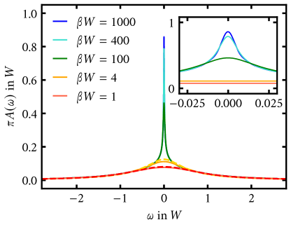
Figure 1: The ext-DEOM simulation results of the impurity spectral function $A(\omega)$ at different temperatures: $\beta W=$ 1, 4, 100, 400 and 1000 with coupling constant $J=0.3W$. The perturbative results are plotted in dash lines for $\beta W=1$ and $4$. Inset is the zooming in on the peaks. The Friedel sum is $\pi A(\omega=0,T=0)=1$ in unit of $W$.

IV Concluding remarks

Obtaining and understanding dynamics for quantum impurity system are of great significance in various fields. The DEOM formalism is proposed and used as a standard theoretical framework to describe the dynamics of impurities embedded in environments. In this work, an extended DEOM is presented to deal with quadratic couplings for electronic open quantum systems. The full DEOM formalism offers a powerful tool for studying the noval behaviors in electronic impurity systems and is particularly useful in situations where nonequilibrium and strongly correlated effects are significant.

Numerical simulations are carried out to investigate the temperature dependence of the Kondo resonance in quantum dots represented by the Kondo model, demonstrating the usefulness of the proposed extension. It is anticipated that fermionic ext-DEOM dissipaton theories would become essential towards the characterization of electronic quantum impurities, whose formulations cover the Schrödinger picture, the Heisenberg picture, and further the imaginary–time calculations. [59]

Despite these advantages, DEOM faces a huge computational effort in calculating the impurity properties at extremely low temperatures, compared to other methods that can used to treat the Kondo model, for example, the numerical renormalization group method. This largely limits the applications of DEOM in these scenarios. Many efforts are devoted to alleviate this difficulty; see Refs. 46 and 59 for more information.

Supplemental material

The supplementary material is available at:

• The relevant code using in this work can be found in the Moscal 2.0 project (fermi-quad module) at https://git.lug.ustc.edu.cn/czh123/moscal2.0.

- [1] J. Kondo, Phys. Rev. 169, 437 (1968).
- [2] G. J. Small, in Spectroscopy and Excitation Dynamics of Condensed Molecular Systems, edited by V. M. Agranovich and R. M. Hochstrasser, page 515, North-Holland Publishing Company, Amsterdam, 1983.
- [3] R. Žitko and J. Bonča, Phys. Rev. B 74, 045312 (2006).
- [4] A. V. Balatsky, I. Vekhter, and J.-X. Zhu, Rev. Mod. Phys. 78, 373 (2006).
- [5] R. H. Foote, D. R. Ward, J. R. Prance, J. K. Gamble, E. Nielsen, B. Thorgrimsson, D. E. Savage, A. L. Saraiva, M. Friesen, S. N. Coppersmith, and M. A. Eriksson, Appl. Phys. Lett. 107, 103112 (2015).
- [6] S. Hershfield, J. H. Davies, and J. W. Wilkins, Phys. Rev. Lett. 67, 3720 (1991).
- [7] G.-H. Ding and T.-K. Ng, Phys. Rev. B 56, R15521 (1997).
- [8] G.-H. Ding and T.-K. Ng, Phys. Rev. B 56, R15521 (1997).
- [9] A. Schiller and S. Hershfield, Phys. Rev. B 58, 14978 (1998).
- [10] N. L. Dickens and D. E. Logan, J. Phys.: Condens. Matter 13, 4505 (2001).
- [11] H. G. Luo, T. Xiang, X. Q. Wang, Z. B. Su, and L. Yu, Phys. Rev. Lett. 92, 256602 (2004), Reply: 96, 019702 (2006).
- [12] K. Le Hur, P. Doucet-Beaupré, and W. Hofstetter, Phys. Rev. Lett. 99, 126801 (2007).
- [13] J. T. Li, W.-D. Schneider, R. Berndt, and B. Delley, Phys. Rev. Lett. 80, 2893 (1998).
- [14] D. A. Ruiz-Tijerina, E. Vernek, and S. E. Ulloa, Phys. Rev. B 90, 035119 (2014).
- [15] O. Újsághy, J. Kroha, L. Szunyogh, and A. Zawadowski, Phys. Rev. Lett. 85, 2557 (2000).
- [16] M. Hamasaki, Phys. Rev. B 69, 115313 (2004).
- [17] S. Schmitt, T. Jabben, and N. Grewe, Phys. Rev. B 80, 235130 (2009).
- [18] A. Isidori, D. Roosen, L. Bartosch, W. Hofstetter, and P. Kopietz, Phys. Rev. B 81, 235120 (2010).
- [19] G. Cohen and E. Rabani, Phys. Rev. B 84, 075150 (2011).
- [20] N. Tsukahara, S. Shiraki, S. Itou, N. Ohta, N. Takagi, and M. Kawai, Phys. Rev. Lett 106, 187201 (2011).
- [21] C. P. Orth, D. F. Urban, and A. Komnik, Phys. Rev. B 86, 125324 (2012).
- [22] Z. Q. Zhang, S. Li, J. T. Lü, and J. Gao, Phys. Rev. B 96, 075410 (2017).
- [23] E. Gull, A. J. Millis, A. I. Lichtenstein, A. N. Rubtsov, M. Troyer, and P. Werner, Rev. Mod. Phys. 83, 349 (2011).
- [24] R. Härtle, G. Cohen, D. R. Reichman, and A. J. Millis, Phys. Rev. B 92, 085430 (2015).
- [25] K. G. Wilson, Rev. Mod. Phys. 47, 773 (1975).
- [26] M. Yoshida, M. A. Whitaker, and L. N. Oliveira, Phys. Rev. B 41, 9403 (1990).
- [27] T. A. Costi, Phys. Rev. B 55, 3003 (1997).
- [28] R. Bulla, A. C. Hewson, and T. Pruschke, J. Phys.: Cond. Matt. 10, 8365 (1998).
- [29] R. Peters, T. Pruschke, and F. B. Anders, Phys. Rev. B 74, 245114 (2006).
- [30] F. B. Anders, J. Phys.: Condens. Matter 20, 195216 (2008).
- [31] F. B. Anders and A. Schiller, Phys. Rev. Lett. 95, 196801 (2005).
- [32] L. Fritz, S. Florens, and M. Vojta, Phys. Rev. B 74, 144410 (2006).
- [33] S. Nishimoto and E. Jeckelmann, J. Phys.: Condens. Matter 16, 613 (2004).
- [34] L. Merker, A. Weichselbaum, and T. A. Costi, Phys. Rev. B 86, 075153 (2012).
- [35] J. Prior, A. W. Chin, S. F. Huelga, and M. B. Plenio, Phys. Rev. Lett. 105, 050404 (2010).
- [36] A. Nüßeler, I. Dhand, S. F. Huelga, and M. B. Plenio, Phys. Rev. B 101, 155134 (2020).
- [37] M. R. Jørgensen and F. A. Pollock, Phys. Rev. Lett. 123, 240602 (2019).
- [38] M. Richter and S. Hughes, Phys. Rev. Lett. 128, 167403 (2022).
- [39] M. Cygorek, M. Cosacchi, A. Vagov, V. M. Axt, B. W. Lovett, J. Keeling, and E. M. Gauger, Nat. Phys. 18, 662 (2022).
- [40] G. Cohen, E. Gull, D. R. Reichman, and A. J. Millis, Phys. Rev. Lett. 115, 266802 (2015).
- [41] H.-T. Chen, G. Cohen, and D. R. Reichman, The Journal of chemical physics 146, 054105 (2017).
- [42] Z. Cai, J. Lu, and S. Yang, Communications on Pure and Applied Mathematics 73, 2430 (2020).
- [43] C. Bertrand, D. Bauernfeind, P. T. Dumitrescu, M. Maček, X. Waintal, and O. Parcollet, Phys. Rev. B 103, 155104 (2021).
- [44] M. E. Sorantin, D. M. Fugger, A. Dorda, W. von der Linden, and E. Arrigoni, Phys. Rev. E 99, 043303 (2019).
- [45] R. P. Feynman and F. L. Vernon, Jr., Ann. Phys. 24, 118 (1963).
- [46] Y. Tanimura, J. Chem. Phys 153, 020901 (2020).
- [47] Y. Tanimura and R. Kubo, J. Phys. Soc. Jpn. 58, 101 (1989).
- [48] Y. Tanimura, Phys. Rev. A 41, 6676 (1990).
- [49] Y. A. Yan, F. Yang, Y. Liu, and J. S. Shao, Chem. Phys. Lett. 395, 216 (2004).
- [50] Y. Tanimura, J. Phys. Soc. Jpn. 75, 082001 (2006).
- [51] R. X. Xu, P. Cui, X. Q. Li, Y. Mo, and Y. J. Yan, J. Chem. Phys. 122, 041103 (2005).
- [52] R. X. Xu and Y. J. Yan, Phys. Rev. E 75, 031107 (2007).
- [53] J. J. Ding, R. X. Xu, and Y. J. Yan, J. Chem. Phys. 136, 224103 (2012).
- [54] J. S. Jin, X. Zheng, and Y. J. Yan, J. Chem. Phys. 128, 234703 (2008).
- [55] Z. H. Li, N. H. Tong, X. Zheng, D. Hou, J. H. Wei, J. Hu, and Y. J. Yan, Phys. Rev. Lett. 109, 266403 (2012).
- [56] L. Z. Ye, X. L. Wang, D. Hou, R. X. Xu, X. Zheng, and Y. J. Yan, WIREs Comp. Mol. Sci. 6, 608 (2016).
- [57] T. A. Costi, Phys. Rev. Lett. 85, 1504 (2000).
- [58] Y. J. Yan, J. Chem. Phys. 140, 054105 (2014).
- [59] Y. Wang and Y. J. Yan, J. Chem. Phys. 157, 170901 (2022).
- [60] R. X. Xu, Y. Liu, H. D. Zhang, and Y. J. Yan, Chin. J. Chem. Phys. 30, 395 (2017).
- [61] R. X. Xu, Y. Liu, H. D. Zhang, and Y. J. Yan, J. Chem. Phys. 148, 114103 (2018).
- [62] Z.-H. Chen, Y. Wang, R.-X. Xu, and Y. Yan, J. Chem. Phys. 158, 074102 (2023).
- [63] Y. J. Yan, J. S. Jin, R. X. Xu, and X. Zheng, Frontiers Phys. 11, 110306 (2016).
- [64] N. N. Bogoliubov and N. N. Bogoliubov Jr, Introduction to Quantum Statistical Mechanics (Second Edition), World Scientific Publishing Company, 2009.
- [65] A. C. Hewson, The Kondo Problem to Heavy Fermions, Cambridge University Press, Cambridge, 1993.
- [66] G. D. Mahan, Many-Particle Physics, Plenum, New York, 3rd edition, 2000.
- [67] Z. H. Chen, Y. Wang, X. Zheng, R. X. Xu, and Y. J. Yan, J. Chem. Phys. 156, 221102 (2022).
- [68] Zitko, Rok., Nrg ljubljana.
- [69] D. C. Langreth, Phys. Rev. 150, 516 (1966).