Quantum Estimation of the Stokes Vector Rotation for a General Polarimetric Transformation

Abstract

Classical polarimetry is a rich and well established discipline within classical optics with many applications in different branches of science. Ever-growing interest in utilizing quantum resources in order to make highly sensitive measurements, prompted the researchers to describe polarized light in a quantum mechanical framework and build a quantum theory of polarimetry within this framework. In this work, inspired by the polarimetric studies in biological tissues, we study the ultimate limit of rotation angle estimation with a known rotation axis in a quantum polarimetric process, which consists of three quantum channels. The rotation angle to be estimated is induced by the retarder channel on the Stokes vector of the probe state. However, the diattenuator and depolarizer channels act on the probe state, which effectively can be thought of as a noise process. Finally the quantum Fisher information (QFI) is calculated and the effect of these noise channels and their ordering is studied on the estimation error of the rotation angle.

I Introduction

Polarization is a property of a propagating electromagnetic wave which quantifies the direction of the oscillations of the electric field. This property of the electromagnetic waves are exploited in a diverse set of technological applications in materials science [1, 2, 3, 4, 5], astronomy [6, 7], medical sciences [8, 9, 10, 11, 12], and quantum information [13]. Interaction with a medium can alter the polarization state of light. A simple framework for calculating the transformation of polarized light under different optical elements is Jones matrix calculus [14]. In this framework the polarized light is modeled using a $2\times 1$ vector and the optical elements causing the polarized light to undergo linear transformations is modeled by $2\times 2$ matrices. However, Jones calculus is only applicable for fully polarized states. A more general framework is the Mueller matrix calculus, which can be used to model partially polarized states and depolarizing transformations as well [14]. In Mueller calculus the polarization states are represented by the Stokes vectors which are $4\times 1$ vectors and optical elements are modeled using $4\times 4$ Mueller matrices.

Optical polarimetry is a field of study and a set of techniques concerning measurement and interpretation of the polarization information of light. Studying the polarization of light before and after it interacts (transmission, reflection, or scattering) with a medium, one can infer several optical and geometric properties of the sample. Based on the optical properties of the material under study different polarimetry technique might be used, e.g. transmission polarimetry , ellipsometry, etc. Mueller polarimeters measure the complete polarization state of light using the 16 elements of the Mueller matrix [15]. Non-invasive nature and high precision of polarimetry makes it suitable for studying sensitive samples. Ellipsometry is widely used for many applications including measurement of the refractive index and thickness of thin films [3]. Another application of polarimetry, is the measurement of the polarization parameters of the human eye and thickness of the retinal nerve fiber layer (RNFL), which can be used to diagnose glaucoma [12, 16, 17, 18, 19]. The basic principle is that, RNFL is birefringent, therefore it can be modeled by a linear retarder which rotates the Stokes vector of the incoming probe state. Estimation of this rotation angle therefore, yields an estimate of the thickness of the RNFL [17, 18, 19].

With growing interest in quantum metrology, there have been attempts to utilize quantum resources for accurate measurement of physical parameters. Estimation of rotation angles is also of a great interest in quantum communication for studies in alignment of the reference frames of the communicating parties[20, 21, 22, 23, 24, 25, 26, 27, 28]. Other than rotation sensing, there are also attempts to utilize quantum resources for specific polarimetric tasks in the literature [29, 30, 31, 32]. Goldberg et al. [33, 34, 35, 36] have studied changes in quantum polarization and have established a quantum mechanical framework for polarimetry. In this framework the Stokes parameters are promoted to operators and by imposing the requirement that the Stokes vector of the expected values of these operators must transform according to the relevant Mueller matrices, the corresponding quantum polarization channels are introduced and investigated.

Based on the framework developed in [33] and inspired by the studies in vision and applications of metrology in biological systems [8, 9, 10, 11, 12, 16, 17, 18, 19, 37, 38], we aim to assess the feasibility of using quantum polarimetry for estimation of rotation angle of stokes vector due to a birefringent medium, modeled by a linear retarder, in presence of diattenuation and depolarization. Studies on biological tissues have shown that, although the polar decomposition of Mueller matrix [39] in tissue polarimetry can yield reliable polarization properties in classical regime, however this decomposition does not correspond to the underlying physical reality [9, 40, 41]. Therefore it is crucial to study the precision limits in quantum polarimetry considering non-commutivity of the elementary components of the Mueller matrix, which implies considering different composition orders of the quantum polarization channels.

This manuscript is organized as follows. In Section II we introduce concepts in quantum polarimetry such as Stokes operators and their transformations due to polarization channels. In basic concepts in quantum metrology, i.e. Section III QFI and quantum Cramer-Rao bound (QCRB) are introduced. In Section IV the results of our calculations for QFI using N00N and coherent states as probe states are given and finally in Section V we present our conclusions.

II Quantum Description of Polarized Light and Polarization Transformations

In a quantum optical setting, each polarization mode can be thought of as a harmonic oscillator. One can write a general pure state of light by acting the creation operators of the horizontal and vertical polarization modes on the vacuum state.

$$\left|\psi\right\rangle=\sum_{m,n}c_{m,n}\left|m,n\right\rangle,$$ (1)

$$\left|m,n\right\rangle\equiv\hat{a}^{\dagger}\vphantom{a}{}^{m}\hat{b}^{\dagger}\vphantom{a}{}^{n}\left|\text{vac}\right\rangle/\sqrt{m!n!}.$$

We take $\hat{a}$ and $\hat{b}$ to be the annihilation operators of the horizontal and vertical polarization modes respectively. These operators satisfy the bosonic commutation relations. Using the field operators of the horizontal and vertical polarization modes we can define the Stokes operators as

$$\hat{S}_{0}=\left(\hat{a}^{\dagger}\hat{a}+\hat{b}^{\dagger}\hat{b}\right)/2\quad\hat{S}_{x}=\left(\hat{a}^{\dagger}\hat{b}+\hat{b}^{\dagger}\hat{a}\right)/2,$$ (2)

$$\hat{S}_{y}=-\text{i}\left(\hat{a}^{\dagger}\hat{b}-\hat{b}^{\dagger}\hat{a}\right)/2\quad\hat{S}_{z}=\left(\hat{a}^{\dagger}\hat{a}-\hat{b}^{\dagger}\hat{b}\right)/2.$$

The Stokes operators are quantum generalizations of the Stokes parameters, which are promoted to an operator status. These operators obey the following $\mathfrak{su}(2)$ algebraic relations

$$\left[\hat{S}_{i},\hat{S}_{j}\right]=\text{i}\sum_{k=1}^{3}\epsilon_{ijk}\hat{S}_{k}$$ (3)

$$\hat{S}_{x}^{2}+\hat{S}_{y}^{2}+\hat{S}_{z}^{3}=\hat{S}_{0}\left(\hat{S}_{0}+1\right).$$

Similar to the classical case, one can use the stokes operators to define a semiclassical degree of polarization (DOP) [34].

$$\mathbb{P}_{s}=\frac{\lvert\langle\hat{\mathbf{S}}\rangle\rvert}{\langle\hat{S}_{0}\rangle}=\frac{\sqrt{\langle\hat{S}_{1}\rangle^{2}+\langle\hat{S}_{2}\rangle^{2}+\langle\hat{S}_{3}\rangle^{2}}}{\langle\hat{S}_{0}\rangle}\,.$$ (4)

Here, $\langle\hat{S}_{i}\rangle=\text{Tr}[\hat{\hat{\rho}}\hat{S}_{i}]$ denotes the expected value of the operator $\hat{S}_{i}$ and $\hat{\mathbf{S}}$ is the normalized Stokes vector. In quantum mechanics, a general transformation of an operator is described by a completely positive trace preserving (CPTP) dynamical map which are also dubbed as a quantum channel. Kraus’ theorem states that any quantum channel can be described by a set of Kraus operators $\{K_{l}\}$ such that,

$$\hat{S}_{\mu}\to\sum_{l}\hat{K}_{l}^{\dagger}\hat{S}_{\mu}\hat{K}_{l}.$$ (5)

In order for the expectation values of the Stokes operators transform according to the classical Mueller description, the following condition must be satisfied.

$$\langle S_{\mu}\rangle\to\sum_{\nu=0}^{3}M_{\mu\nu}\langle S_{\nu}\rangle,$$ (6)

For both Eq. 5 and Eq. 6 to hold, we can impose the condition that the Stokes operators should transform in the same way as the Stokes parameters [33],

$$\sum_{l}\hat{K}_{l}^{\dagger}\hat{S}_{\mu}\hat{K}_{l}=\sum_{\nu}M_{\mu\nu}\hat{S}_{\nu}.$$ (7)

It is shown that if the Mueller matrix is not singular, one can decompose it into a product of three elementary matrix factors with well-defined polarimetric properties: a retarder, a diattenuator and a depolarizer [39]. In Eq. 8 the standard Lu-Chipman decomposition is shown.

$$M=M_{d}M_{R}M_{D}.$$ (8)

Here, $M_{D}$, $M_{R}$ and $M_{d}$ are the elementary Mueller matrices for the diattenuator, retarder and depolarizer components respectively. Firstly, it must be noted that this decomposition is made solely for interpreting the polarimetric data and extracting physical parameters more conveniently by capturing the effective polarization transformation and doesn’t necessarily describe the actual physical underlying process. This is specially the case for biological tissues for which the depolarization, diattenuation and retardation effects are likely to occur simultaneously [9, 40, 41]. Secondly, due to the fact that in general matrix product is non-commutative, the decomposition order given in Eq. 8 is not the only decomposition that one can make out of the original Mueller matrix. Based on the optical characteristics of the sample, there exist a multitude of ways to break down the total Mueller matrix into a combination of the elementary ones of which Eq. 8 is only a special case [9, 39, 40, 41, 42, 43, 44, 45, 46, 47]. Based on Eq. 7 we can describe the quantum mechanical polarization channels as [33],

$$\varepsilon(\hat{\rho})=\varepsilon_{d}\circ\varepsilon_{R}\circ\varepsilon_{D}(\hat{\rho}),$$ (9)

in which $\varepsilon_{D}$, $\varepsilon_{R}$ and $\varepsilon_{d}$ are the diattenuator, retarder and depolarizer channels, respectively. A schematic representation of this channel is given in Fig. 1.

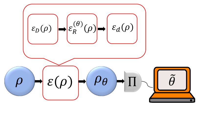
Figure 1: A schematic representation of the general polarization channel. In this figure the order of the action of the diattunator, retarder and depolarizer channels follows the standard Li-Chipman form.

The retarder channel rotates the Stokes vector which also acts as a unitary rotation on the density matrix [27, 33, 35, 36].

$$\varepsilon_{R}(\hat{\rho})=\hat{R}(\theta,\mathbf{n})\hat{\rho}\hat{R}^{\dagger}(\theta,\mathbf{n}).$$ (10)

Here, the operator $\hat{R}$ is given by

$$\hat{R}(\theta,\mathbf{n})=\text{exp}(i\theta\hat{\mathbf{S}}.\mathbf{n}),$$ (11)

in which $\mathbf{n}$ is the direction of rotation and $\theta$ is the angle of rotation. The diattenuator channel can be modeled by a sequential application of rotation operators in an enlarged Hilbert space containing two ancillary modes and tracing out the ancillary modes. It is given by [33, 35, 36]

$$\varepsilon_{D}(\hat{\rho})=\text{Tr}_{v_{1},v_{2}}[\hat{U}_{D}(\hat{\rho}\otimes|\text{vac}\rangle_{v_{1},v_{2}}{}_{v_{1},v_{2}}\langle\text{vac}|)\hat{U}_{D}^{\dagger}],$$ (12)

in which $v_{1}$ and $v_{2}$ are the ancillary modes and the operator $\hat{U}_{D}$ is

$$\begin{split}\hat{U}_{D}=\hat{R}_{a,b}^{\dagger}(0,\beta,\gamma)\hat{R}_{b,v_{2}}(0,-2cos^{-1}(0,\sqrt{r},0))\\ \hat{R}_{a,v_{1}}(0,-2cos^{-1}(0,\sqrt{q},0))\hat{R}_{a,b}(0,\beta,\gamma).\end{split}$$ (13)

Here, $\hat{R}_{a,b}$ denotes a rotation operator between modes $a$ and $b$ parametrized by the Euler angles $(0,\beta,\gamma)$. $\hat{R}_{a,v_{1}}$ and $\hat{R}_{b,v_{2}}$ are rotations between modes $a$ and $v_{1}$ and $b$ and $v_{2}$ respectively with their respective attenuation parameters $q$ and $r$. Finally the depolarizer is given by [33]

$$\varepsilon_{d}(\hat{\rho})=p\hat{\rho}+(1-p)\sum_{M}p_{N}\frac{\hat{\mathds{1}}_{N}}{N+1},$$ (14)

in which $p$ is the depolarization parameter and $p_{N}$ is the weight of the density matrix in each photon number subspace. For our purposes, we can express depolarization as a convex sum of two rotation operators [35, 36]. For the sake of simplicity we take two rotation operators.

$$\varepsilon_{d}(\hat{\rho})=\frac{\hat{R}_{1}\hat{\rho}\hat{R}_{1}^{\dagger}+\hat{R}_{2}\hat{\rho}\hat{R}_{2}^{\dagger}}{2}.$$ (15)

III Quantum Parameter Estimation and QCRB

In this section we introduce some of the fundamental results for quantum single parameter estimation. Assume that through a process, the parameter $\theta$ gets encoded on a quantum state. For a parameterized state the lower bound for the variance of any unbiased estimator $\tilde{\theta}$ of the parameter, is given by the QCRB [48, 49, 50, 51, 52, 53].

$$(\Delta\tilde{\theta})^{2}\geq\frac{1}{\nu\mathcal{F}_{Q}(\theta)}.$$ (16)

Here, $\mathcal{F}_{Q}$ is the QFI and $\nu$ is the number of measurement repetitions. QFI is a generalization of the classical Fisher information (CFI) which is defined as the expectation value of the squared derivative of the logarithm of the probability distribution. For a pure state QFI is defined as,

$$\mathcal{F}_{Q}(\theta)=4[\langle\partial_{\theta}\psi|\partial_{\theta}\psi\rangle-|\langle\partial_{\theta}\psi|\psi\rangle|^{2}].$$ (17)

For a mixed state, one can define QFI using the symmetric logarithmic derivative (SLD) operator as

$$\mathcal{F}_{Q}(\theta)=\text{Tr}[\hat{\rho}\hat{L}_{\theta}^{2}].$$ (18)

SLD is implicitly defined by the following equation

$$\partial_{\theta}\hat{\rho}=\frac{\hat{L}_{\theta}\hat{\rho}+\hat{\rho}\hat{L}_{\theta}}{2}.$$ (19)

By expressing $\hat{L}_{\theta}$ in the eigenbasis of $\hat{\rho}$ one can write QFI as

$$\mathcal{F}_{Q}(\theta)=2\sum_{k,l}\frac{|\langle k|\partial_{\theta}\hat{\rho}|l\rangle|^{2}}{\lambda_{k}+\lambda_{l}}.$$ (20)

Here, $k$, $l$ and $\lambda_{k}$, $\lambda_{l}$ are the eigenvalues and eigenvectors of $\hat{\rho}$.

IV Results

In this section we numerically calculate the QFI in order to determine the rotation angle measurement precision. In all of our calculations the rotation angle to be estimated is $\theta=0.01$ with the rotation direction $(\Theta,\Phi)=(0,0)$ in polar coordinates. The probe states have been considered for this task are the coherent and N00N states which are known to saturate the standard quantum limit (SQL) and Heisenberg limit (SQL) for this task considering small rotation angles [27]. As a reference, our numerical results for the QFI in case of no noise is presented in Fig. 2.

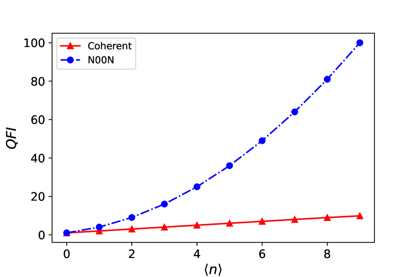
Figure 2: QFI for rotation angle vs average photon number calculated for coherent state (solid line with triangular data poins in red) and N00N state (dash dotted line with circular data poins in blue). Coherent state and N00N state saturate the HL respectively

It is instructive to assess the performance of these states by considering the effect of each of the noise channels on the estimation precision of the rotation angle of the Stokes vector. Therefore, in LABEL:retdep we will study the effect of the depolarization channel on the QFI for the rotation angle and in LABEL:retdepdia the joint effect of depolarization and diattenuation is considered. In both of these cases the ordering of the implementation of the channels is also considered. Using the terminology common in the classical polarimetry, we will call $\varepsilon_{for}(\hat{\rho})=\varepsilon_{d}\circ\varepsilon_{R}\circ\varepsilon_{D}(\hat{\rho})$ as the ”forward” decomposition and $\varepsilon_{rev}(\hat{\rho})=\varepsilon_{d}\circ\varepsilon_{R}\circ\varepsilon_{D}(\hat{\rho})$ as the backward decomposition.

IV.1 Noisy Rotation Sensing with Depolarization

In this section we calculate the QFI for the rotation angle in both forward and reverse processes without considering the effect of diattenuation, focusing only on depolarization. The results of out calculations are shown in Fig. 3. The rotation axes for $\hat{R}_{1}$ and $\hat{R}_{2}$ are $(\Theta,\Phi)=(\pi/2,\pi/2)$ and $(\Theta,\Phi)=(0,0)$ respectively and the rotation angle for both of them is set to 0.01. It is evident that for N00N state, both in forward and reverse processes the overall performance has decreased and the scaling with the average photon number is not strictly monotonic in the case of reverse process. For the case of coherent state, in forward process there is no appreciable change in QFI compared with the noiseless case. However, in the reverse process, we witness a noise assisted increase in QFI. The results show that N00N state is advantageous for the task of rotation sensing, compared with the coherent state.

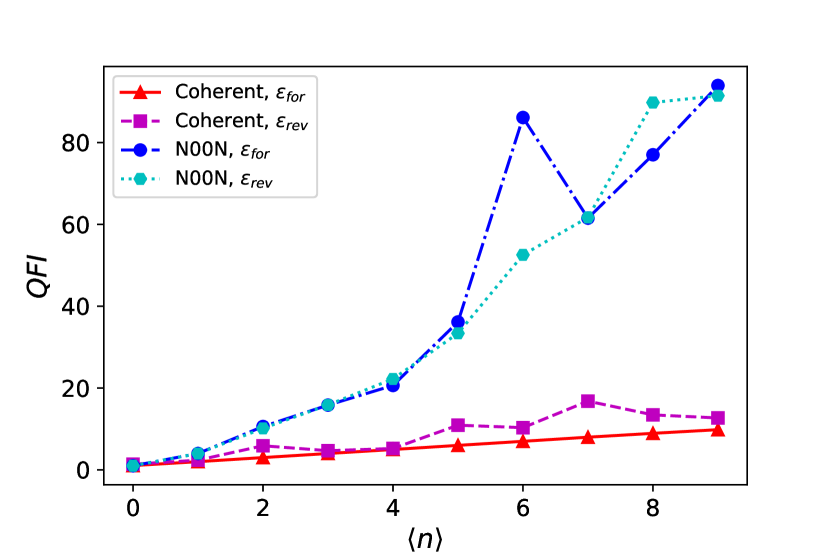
Figure 3: QFI for rotation angle in presence of depolarization noise vs average photon number. Calculations are for coherent state in forward (solid line with triangular data poins in red) and reverse (dashed line with square data poins in magenta) processes and for N00N state in forward (dash dotted line with circular data poins in blue) and reverse (dotted line with triangular data poins in cyan) processes.

IV.2 Noisy Rotation Sensing with Depolarization and Diattenuation

Finally, we calculate the QFI for the rotation angle vs the average photon number of the probe states considering both depolarization and diattenuation channels in forward and reverse decomposition channels. The results are shown in Fig. 4. The parameters of rotation are identical with the ones chosen in the previous subsection and diattenuation parameters are $q=0.9$ and $r=1$. The results show that, even though the scaling is diminished, N00N state still results in larger values for QFI.

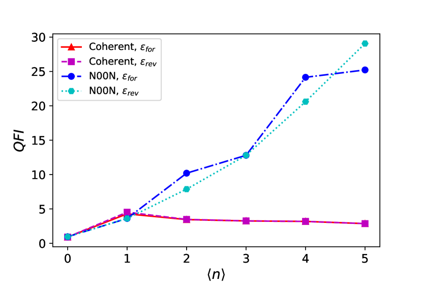
Figure 4: QFI for rotation angle in presence of depolarization and diattenuaion noise vs average photon number. Calculations are for coherent state in forward (solid line with triangular data poins in red) and reverse (dashed line with square data poins in magenta) processes and for N00N state in forward (dash dotted line with circular data poins in blue) and reverse (dotted line with triangular data poins in cyan) processes.

V Conclusion

In conclusion, we studied the precision limits for single parameter estimation of the rotation angle of the Stokes vector in a polarimetric setup, within the framework of recently developed quantum polarimetry. We have incorporated the effects of depolarization and diattenuation channels within our numerical calculations and considered different orders of implementations of these channels. The results show that QFI generally deteriorates upon implementation of the polarimetric depolarization channel. However this statement is not valid in every case, as we have witnessed an increase in QFI using the coherent state as a probe in the reverse decomposition of our channel when diattenuation was disregarded. As expected, implementing diattenuation decreases QFI for all cases. However, our results demonstrate that the advantage of N00N state over coherent state still persists upon implementation of diattenuation and depolarization in both forward and reverse processes.