Thermal signature of helical molecule: Beyond nearest-neighbor electron hopping
Abstract
We investigate, for the first time, the thermal signature of a single-stranded helical molecule, subjected to a transverse electric field, by analyzing electronic specific heat (ESH). Depending on the hopping of electrons, two different kinds of helical systems are considered. In one case the hopping is confined within a few neighboring lattice sites which is referred to as short-range hopping (SRH) helix, while in the other case, electrons can hop in all possible sites making the system a long-range hopping (LRH) one. The interplay between helicity and the electric field is quite significant. Our detailed study shows that, in the low-temperature limit, the SRH helix is more sensitive to temperature than its counterpart. Whereas, the situation gets reversed in the limit of high temperatures. The thermal response of the helix can be modified selectively by means of the electric field, and the difference between specific heats of the two helices gradually decreases with increasing the field strength. The molecular handedness (viz, left-handed or right-handed) rather has no appreciable effect on the thermal signature. Finally, one important usefulness of ESH is discussed. If the helix contains a point defect, then by comparing the results of perfect and defective helices, one can estimate the location of the defect, which might be useful in diagnosing bad cells and different diseases.
I Introduction
During the past few years, helical molecules have been actively used for designing different efficient nanoscale charge and spin-based electronic devices dev1 ; dev2 ; dev3 . Starting from spin-specific electron transmission, current rectification, magneto-resistive behavior, and many other operations are performed with great efficiency hel1 ; hel2 ; hel3 ; hel4 ; hel5 ; hel6 ; hel7 ; hel8 ; sp1 ; sp2 ; sp3 ; sp4 ; sp5 ; recti ; sp6 ; sp7 ; gmr ; thermo . All these functionalities are directly involved with the unique and diverse characteristic features of helical molecular systems. Depending on the geometrical structure, essentially two different classes of helical molecules are defined. In one case, electrons are able to hop from one atomic site to its few neighboring sites, making the system a short-range hopping helix hel5 . Whereas, in another case, electrons can hop in all possible sites yielding a long-range hopping helix hel5 ; hel6 . The most common realistic examples of SRH and LRH helices are the single-stranded DNA and protein molecules respectively hel6 . Due to the existence of higher-order electron hopping, these systems exhibit unusual phenomena compared to the traditional nearest-neighbor hopping (NNH) model.
Though substantial progress has been made in studying electron and spin-dependent transport phenomena considering different real biological helical molecules as well as tailor-made helical systems bio1 ; bio2 ; bio3 , thermal signature in helical systems has not been studied so far to the best of our concern, which thus definitely needs to be addressed. In our present work, we explore it by investigating electronic specific heat (ESH). To date, most of the theoretical studies are confined to only the nearest-neighbor hopping (NNH) of electrons sh1 ; sh2 ; sh3 ; sh4 ; sh5 ; sh6 ; sh7 ; sh8 ; sh9 ; sh10 ; sh11 , and no attempt has been made considering a system possessing higher-order hopping of electrons. Our primary aim is to inspect the thermal responses of SRH and LRH helices.
To explore the role of disorder and for a possible tuning of ESH, we apply an electric field perpendicular to helix axis (see Fig. 1). In presence of this field, the system becomes a correlated disordered one efl . Because of the geometrical conformation, site energies of the helix are modulated lhrh in a cosine form, following the well-known Aubry-André-Harper (AAH) ab1 ; ab2 ; ab3 ; ab4 ; ab5 model. This is a special class of correlated disorder that exhibits several non-trivial signatures in the context of electronic localization loc1 ; loc2 ; loc3 ; loc4 . Unlike a one-dimensional uncorrelated (random) disordered lattice where all the eigenstates are localized irrespective of the disorder strength dis1 ; dis2 , an AAH system goes to the localized phase from the conducting one beyond a finite disorder strength ab1 ; ab2 ; ab3 . More interesting phenomena are observed when the system is described beyond the nearest-neighbor hopping sdsarma . The modulation in site energies directly influences the energy eigenspectrum, and thus, the electronic specific heat as it depends on the density of states. It will be interesting to check the interplay between the helicity, higher-order electron hopping, and the electric field on ESH.
We describe the helical molecular system within a tight-binding (TB) framework, that gives a simple level of description hel5 ; hel7 ; sp7 . Diagonalizing the TB Hamiltonian matrix for a finite-size helix, we calculate the average energy, and then taking the derivative of the average energy with respect to temperature, specific heat is computed sh3 ; sh6 ; sh7 . From our exhaustive numerical analysis, we find that an SRH helix is more sensitive to temperature compared to the LRH one, in the low-temperature limit. While, in higher temperatures, the response gets reversed. Though the features of both these temperature regimes still persist in presence of the electric field, the difference in specific heats between the SRH and LRH helices gets reduced gradually with increasing the field strength. It is worth pointing out that the thermal response can be modified selectively through the electric field. But the handedness does not have any such significant effect. All these aspects are critically discussed in our work with suitable arguments.
Finally, we concentrate on one important usefulness of the specific heat. It has already been highlighted by some researchers that from the concept of ESH different kinds of neurodegenerative diseases shd like Parkinson, Alzheimer, Creutzfeldt-Jakob, and many more might be diagnosed. Here in our helices we include a point defect at an arbitrary lattice site and try to figure it out the location of the defect by comparing the results of perfect and defected helices. At some level, it can be done, and we believe that this protocol can be utilized in diagnosing defective cells and different diseases.
The rest part of the work is organized as follows. The helical systems and the theoretical framework for the calculations are given in Sec. II. All the numerical results are presented and thoroughly scrutinized in Sec. III. In the end, Sec. IV includes a summary of the findings.
II Physical system, tight-binding Hamiltonian and theoretical formulation
II.1 Helix geometry and tight-binding Hamiltonian
The physical system for which the thermal signature is discussed in this work is schematically given in Fig. 1.
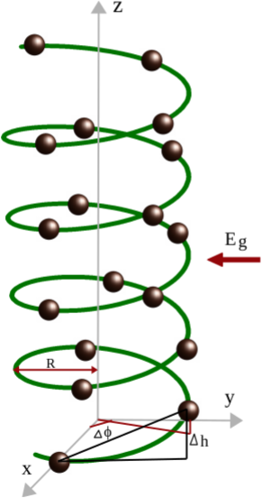
It is a right-handed helix. Two important parameters are there that essentially describe a helical structure, and they are twisting angle (measures how the geometry is twisted) and the stacking distance between two successive lattice sites hel5 ; sp7 . Depending on the factor , usually two kinds of helices are taken into account. When the distance between the neighboring sites is small (viz, is low), electrons can easily hop from one site to all other possible sites of the geometry making the system a long-range hopping (LRH) helix. While, for the other case, where is high i.e., the atoms are largely separated, the hopping is confined within a few neighboring atomic sites, yielding the helix a short range hopping (SRH) one. Though structurally both LRH and SRH helices look identical, their behaviors are quite different and in the present work we want to explore the interplay between these two kinds of electron hopping on thermal signature.
An electric field is applied along the perpendicular direction of the helix axis. The main reasons for applying to such a field are two-fold. First, in presence of this field the system becomes a correlated (not random) disordered one sp7 ; efl , and thus the effect of disorder can be checked. The interplay between disorder and electron hopping on thermal response might be an interesting observation. Second, to inspect how the thermal response can be modified by means the externally tuning parameter. These issues have not been explored so far in the literature.
A tight-binding framework is given to illustrate the helical system. The general form of the TB Hamiltonian of a helix (be it a short-range or a long-range one) reads as
| (1) | |||||
where denotes the site energy of an electron at th lattice site, and , represent the fermionic creation and annihilation operators respectively. is the hopping strength between the sites and . In terms of NNH hopping strength , can be expressed as hel7 ; qfs
| (2) |
where is the decay constant and is the distance of separation between the sites and (). measures the nearest-neighbor distance. The length is expressed in terms of the structural parameters of the helix as hel7 ; qfs
| (3) |
As mentioned above, depending on , and we can get an SRH or LRH helix system.
Now, whenever an electric field is applied perpendicular to the helix axis, the site energies get modulated in a specific form following the relation efl
| (4) |
Here, is the electronic charge and is the gate voltage that is responsible for producing the field. The gate voltage and the electric field are related by the equation efl . The parameter , refereed to as the phase factor, describes the field direction with respect to the positive axis. At this point, it is worth mentioning that the above expression of site energies looks similar to the most well-known Aubry-André-Harper (AAH) model ab1 ; ab2 ; ab3 , where measures the strength of cosine modulation. Thus, our system becomes quite equivalent to AAH model with higher-order hopping of electrons.
II.2 Theoretical formulation
The electronic specific heat is determined by taking the first order derivative of average energy of the system with respect to temperature . At constant volume it is defined as sh3 ; sh6 ; sh7
| (5) |
where is the average energy, and it is expressed as sh3 ; sh6 ; sh7
| (6) |
Here is the th energy eigenvalue that is obtained by numerically diagonalizing the TB Hamiltonian matrix, is the electro-chemical potential, and is the Fermi-Dirac distribution function. At temperature , is given by
| (7) |
where is the Boltzmann constant. Substituting in Eq. 6, and doing some straightforward algebra we get the form of as
| (8) |
As the ESH is directly connected to the average density of states (ADOS) of the system, we also compute it for a clear description of our results. The ADOS is obtained through the operation gf1
| (9) |
where being the total number of lattice sites and denotes the Green’s function of the helix system. The Green’s function is defined as gf1 ; gf2
| (10) |
where .
III Numerical results and discussion
In what follows we present our numerical results which include the characteristics features of electronic specific heat of both the LRH and SRH helices in the electric field free and with field cases. Specifically, we are interested to explore the interplay between the different ranges of electron hopping, molecular chirality, external electric field and related issues. Before starting our results, let us mention the values of the physical parameters those are kept unchanged throughout the discussion. We choose site energy , nearest-neighbor hopping , electro-chemical potential , and the Boltzmann constant . Unless specified otherwise, we compute all the results for right-handed helices considering . All the energies are measured in unit of electron-volt (eV).
As mentioned, the most common and realistic examples of SRH and LRH helices are the single-stranded DNA and protein molecules hel5 , and here in our calculations we set the physical parameters for these helices from the standard data set available in the literature rps . They are described in Table 1. For a clear visualization of how these physical parameters control the electron hopping,
| Model | (Å) | (Å) | (rad) | (Å) |
|---|---|---|---|---|
| SRH | ||||
| LRH |
in Table 2 we present the distances of few neighboring sites of our chosen SRH and LRH helices. Clearly it is seen that for the case of SRH helix, the neighboring distances increase sharply with the site index, and thus the hopping of electrons is confined within a few neighboring atomic sites. Whereas, the situation is quite different for the other helix viz, the LRH one. The distances are almost
| Model | |||||
|---|---|---|---|---|---|
| SRH | |||||
| LRH |
comparable to each other even when we change the site index to a large value. Due to this fact, hopping in all possible sites takes places, which essentially brings non-trivial signatures compared to the usual NNH lattices.
Now we present and analyze our results one by one, those are placed in different sub-sections.
III.1 In absence of external electric field
Let us begin our discussion with Fig. 2 where the variation of electronic specific heat as a function of system temperature is shown both for the SRH and LRH helices, when there is no external electric field i.e., . Several interesting features are obtained those are as follows. In the low-temperature limit, the specific heat sharply increases with temperature and after reaching a maximum it decreases smoothly and eventually drops almost to zero in the limit of high temperatures. This is the common feature of both the SRH and LRH cases, as clearly visible from the curves given in Fig. 2. But the notable thing is that, for the helix
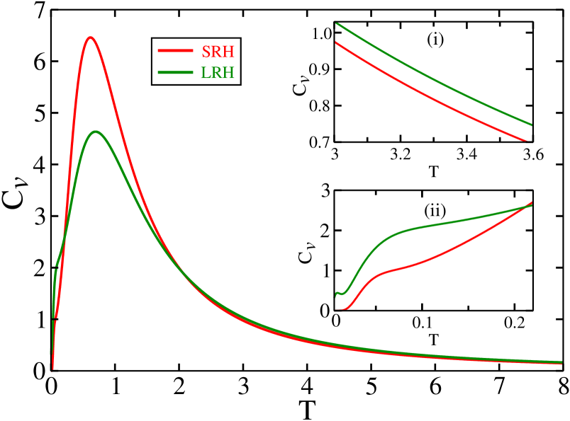
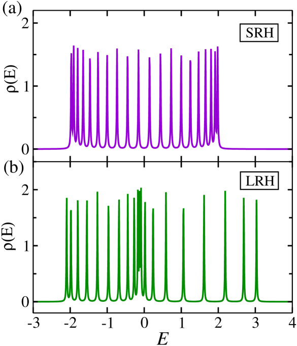
with short-range electron hopping, the ESH becomes reasonably large compared to the other helical system in the low-temperature limit. The difference between the curves gradually decreases with the rise of temperature, and most interestingly it is seen that after a certain temperature range, the ESH of LRH helix dominates the SRH one. This behavior is noticed from the results given in the inset (i) of Fig. 2. The above facts can be explained from the ADOS spectrum presented in Fig. 3, as the ESH is directly connected to the density of states. At zero temperature, the electronic energy levels up to the Fermi energy are fully occupied, while the rest other energy levels are empty. Once the temperature is introduced, a few neighboring energy levels within the range of around the Fermi energy contribute, which enhance the average energy () compared to zero temperature limit. With increasing temperature, more energy levels are accessible and thus the average energy increases, resulting a higher electronic specific heat. This rate of enhancement of for the SRH helix becomes much higher than the LRH one. The reason is that for the SRH helix the energy levels are almost uniformly spaced (see Fig. 3(a)), and hence, more energy levels are accessible within a specific range. Whereas, for the LRH system the levels are largely gapped in the higher energy region above the Fermi level (see Fig. 3(b)), and thus, a less number of eigenenergies is available. The non-uniform spacing of energy levels is the generic feature of higher order electron hopping, and has been reported in several other physical systems with longer-range hopping hel5 ; sp7 . With reducing the hopping range, the levels are packed in a more uniform way, and the complete uniform picture (viz, symmetric energy band spectrum around ) is obtained for the NNH system.
With increasing temperature, the occupation probabilities in the higher energy levels increase gradually and all the energy levels
take part in the average energy . Therefore, further enhancement of with temperature is not that much possible, which yields a reduction of . Eventually, when the temperature is reasonably high, the average energy is almost constant, and under that condition, the specific heat becomes vanishingly small. Since the LRH helix has energy levels at higher energies compared to the SRH one, that is followed by comparing the ADOS spectra given in Fig. 3, in the high-temperature limit the rate of change of with temperature for the LRH helix is higher than the other one, and hence, higher is obtained (for better viewing, see inset (i) of Fig. 2).
From Fig. 2, another interesting feature is noticed at extremely low-temperature limit (viz, when the temperature of the system is almost close to zero). The specific heat for the LRH helix is higher than the SRH one on a too narrow temperature range (see inset (ii) of Fig. 2). This is solely due to the highly packed energy levels of the LRH helix around within the range of (Fig. 3(b)), whereas for the SRH helix no such behavior is available (Fig. 3(a)).
III.2 In presence of external electric field
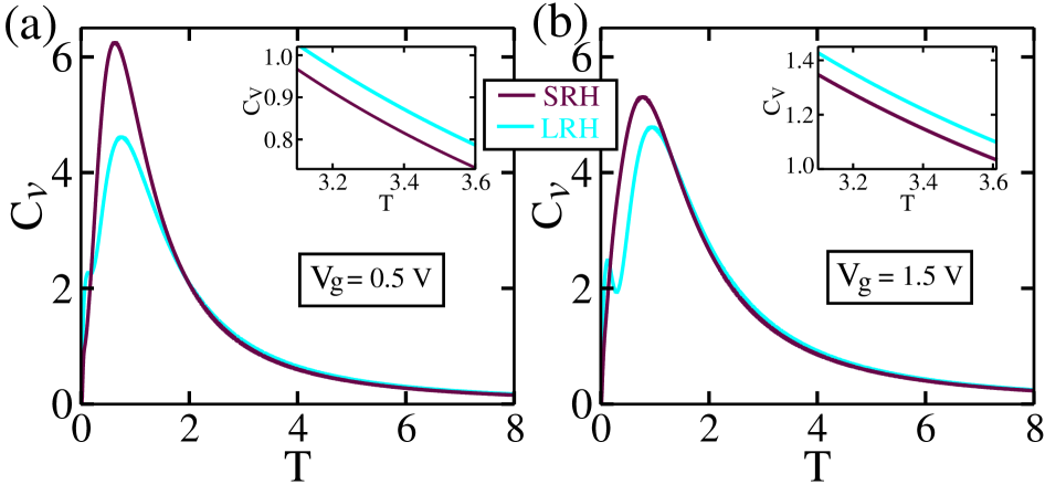
Now we focus on the effects of external electric field on thermal response. Figure 4 shows the dependence of electronic specific heat as a function of temperature for the two different helices when they are subjected to an external electric field viz, when . Nature wise the overall - spectra look identical to what are seen for the field free case i.e., a sharp increment with temperature in the limit of low temperatures, and reaching a maximum, the specific heat decreases and eventually vanishes in the high-temperature limit. The higher value of for the LRH helix compared to the SRH one, which is extremely at the zero temperature limit and in the higher temperature regime, is also similar to the zero-field case. But a careful inspection reveals that, in the presence of the electric field, the difference between the peak values of the - curves associated with the SRH and LRH helices decreases, and it becomes more prominent when the field strength gets enhanced. This behavior can be understood from the following arguments.
The central mechanism is related to the nature of the density of states. In Fig. 5 we plot the ADOS spectra for the two helices at the two gate voltages that are taken in Fig. 4. The effect of electric field is quite fascinating. Whenever an electric field is applied, the site energies are modulated in the cosine form following the relation given in Eq. 4.
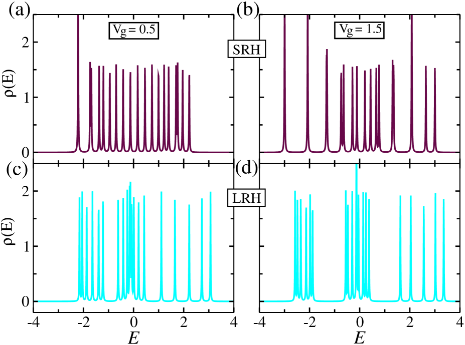
This cosine modulation makes the system a correlated disordered one, analogous to the well-known AAH model ab1 ; ab2 ; ab3 . Due to this specific modulation, the energy spectrum becomes fragmented and gapped. As if the energy levels are arranged in three sub-bands. A more clear picture of it can be seen for a large system size with moderate field strength, and this kind of energy spectrum has already been discussed in a series of papers related to AAH systems ab1 ; ab2 ; ab3 . For large , the effect of correlated disorder dominates the electron hopping, and thus, both the SRH and LRH helices provide quite comparable ADOS spectra (right column of Fig. 5), and hence, their specific heats are not too different (Fig. 4(b)). Whereas, for lower , the ADOS spectra are largely different for the two helices (left column of Fig. 5), and accordingly, the large difference between the specific heats are clearly visible (Fig. 4(a)).
Since the electric field has a strong influence on electronic specific heat, it is indeed required to check how gets modified
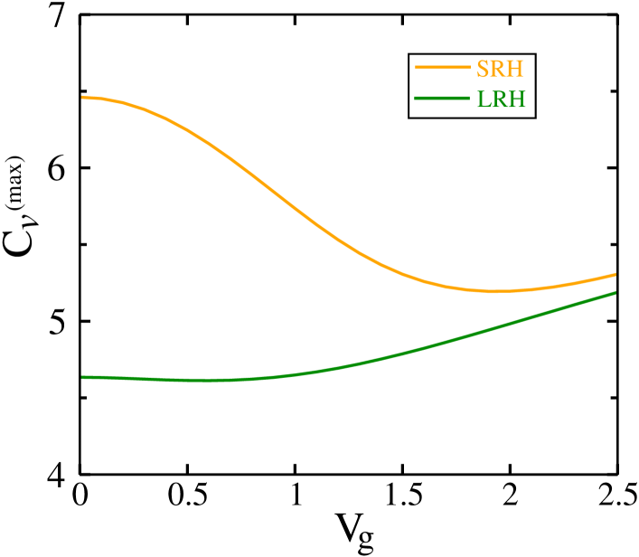
with a continuous variation of the field strength (or we can say by varying the correlated disorder strength). For that, we compute the maximum of (referred to as (max)) and plot it as a function of . For each , we determine in a wide range of temperature and then take the maximum to get (max). The results for both the helices are given in Fig. 6, where the orange and green lines are associated with the SRH and LRH helices respectively.
Following the above argument, interestingly we find that the difference between the specific heats is maximum at , and it gradually decreases with increasing the field strength. For large enough , they are almost close to each other. Thus, the electric field has a strong role to monitor the thermal response.
For the sake of completeness of our analysis, now we discuss the dependencies of the electronic specific heat on different physical parameters that are involved in the system.
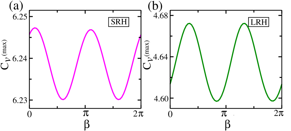
Role of : To inspect how the direction of electric field plays a role on thermal response, in Fig. 7 we plot the variation of (max) with for the SRH and LRH helices when the gate voltage is fixed ta V. The factor , associated with the field direction, appears into the site energy expression through the relation given in Eq. 4. The site energies get modified with the change of , and thus the spectrum of ADOS is also changed, which yields a variation in specific heat. Comparing the results of SRH and LRH systems it is found that in both the cases the variation is not that much significant, but among these two, the LRH helix shows slightly higher response than the SRH one.
Effect of geometrical conformation: It is already established that the stacking distance between the
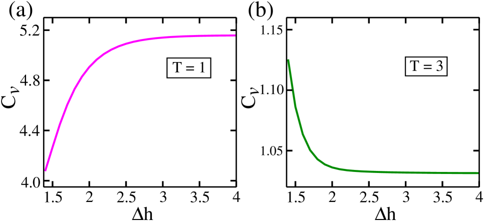
neighboring lattice sites has an important signature in characterizing the range of electron hopping. When is too small, electrons can hop in all possible sites, while for the situation when is quite large, the hopping is confined to a few neighboring sites. As the range of electron hopping has a direct impact on the energy band spectrum, and thus, on the ADOS, here we investigate the role of on ESH. The results are presented in Fig. 8, where two different temperatures, K (low) and K (high) are taken into account. In both the cases, we vary from (chosen value of our LRH helix, as mentioned in Table 1) to a large value up to . Satisfying our previous arguments we notice that in the low-temperature limit, the electronic specific heat increases with i.e., when the system becomes more short-ranged (Fig. 8(a)). On the other hand, in the limit of high-temperature, an opposite signature is found viz, reduction of with (Fig. 8(b)). All these issues are directly connected to the modification of ADOS with the range of electron hopping.
Effect of chirality: At this stage, it is relevant to inspect how the thermal response is sensitive to the chirality of the helical system. The results studied so far are worked out for the right-handed helices. But in presence of the electric field, there is a possibility to have modified ADOS depending on the handedness of the system, as the site energies get changed with the alternation of the handedness from right-handed (RH) to left-handed (LH). To get a left-handed helix, we need to replace by lhrh , keeping all other factors unchanged. Because of this, site energies are different for the RH and LH cases, following the relation given in Eq. 4, and we can expect a change in thermal signature. Here one point needs to be mentioned. In order to have a perfect swapping from one-handedness to the other, we have to take the system size properly such that the helix gets complete full turns. Depending on the structural parameters taken in our SRH and LRH helices (as mentioned in Table 1), we select for the SRH case (two turns) and for the LRH helix (five turns).
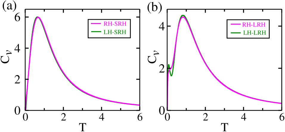
In Fig. 9 we present the results of ESH considering both the right-handed and left-handed helices at a typical gate voltage. What is seen is that, in each hopping case, the specific heats are almost comparable to each other for the right- and left-handed systems. It clearly suggests that with the change of chirality, the ADOS spectrum does not modify appreciably, and hence almost identical curves are obtained for the two different handedness.
III.3 Usefulness of electronic specific heat
Finally, in this sub-section we discuss one usefulness of the ESH. The aim of this part is to inspect whether we can detect any defective lattice site if that exists in the system, by investigating the thermal response. Our scheme is that we introduce a single defect at any arbitrary site, keeping all other sites of the helix identical. The strength of the site energy of the defected site is mentioned by the parameter ( corresponds to the perfect site, as the site energies of all other sites are set at zero). Three different cases are shown, depending on . One is too weak (), and the other two are moderate and quite large. For each of these three cases, we compute the maximum of ESH i.e., (max) and plot it (see Fig. 10) as function of the position of the defective site, denoted by the parameter . The reason for considering too small () in one case is that, here the system is closed to the perfect one, so that we can compare our results with finite . Several important features are obtained those are as follows. For , (max) is almost constant both for the SRH and LRH helices (violet lines of Fig. 10),
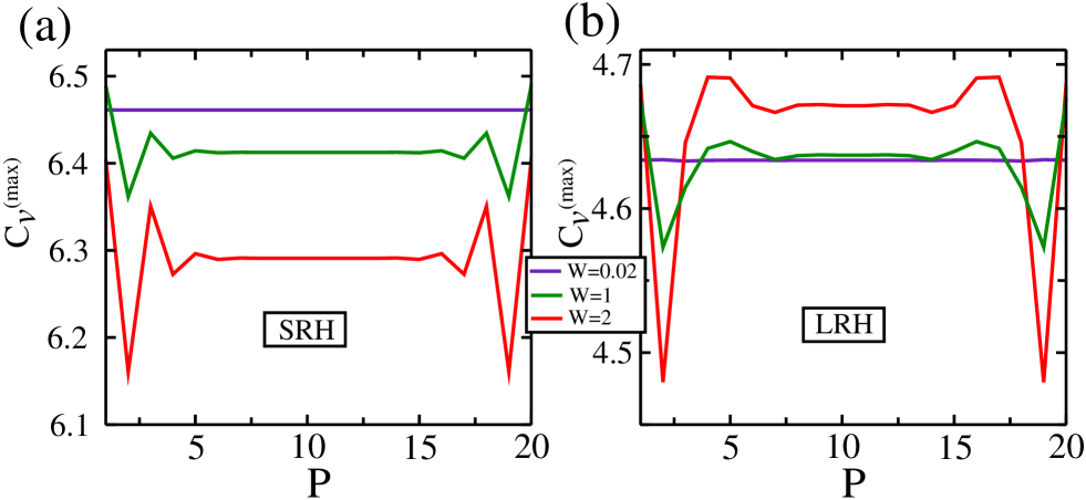
as expected. But for , a sharp change in (max) is obtained when the defective site is located near one edge of the helix (green lines), and the situation becomes more prominent for large (red lines). Though (max)- curves look quite similar for the two helices, the change in ESH with is visible for a large range for the helix with higher order hopping integrals. Comparing the results of perfect and defective helices we can clearly predict which one is defective and also the location can be estimated at some level. Especially when the impurity site is located near any of the two edges, we get a large variation that might be useful for a clear detection.
IV Closing remarks
To conclude, in this work, for the first time, we explore the thermal signature of helical systems by studying electronic specific heat. Though a considerable amount of work involving charge and spin-dependent transport has been done using different kinds of helical systems, the discussion on thermal properties is highly limited. From the knowledge of ESH, we can estimate how a substance is capable of transferring and absorbing energy. Several other aspects can also be specified from the behavior of specific heat like designing cooking utensils, processing temperatures, and to name a few.
Depending on the physical parameters, two different kinds of helical systems are taken into account. Though structurally they look
identical, in one case electron can hop in a few neighboring lattice sites, while in the other case, all possible hoppings are allowed.
To inspect the effect of disorder, we apply an external electric field perpendicular to the helix axis. In presence of this field, the
system maps to correlated disordered one following the well-known AAH model. Simulating the SRH and LRH helices within a TB framework,
we compute ESH by taking the first-order derivative of the average energy. The results are analyzed both for the field-free and
finite-field cases. And in the end, one important usefulness is discussed. The important and new findings of our work are as follows.
In the low-temperature limit, the SRH helix exhibits higher ESH than the LRH one. The situation gets reversed in the limit
of high temperatures.
The difference between the ESHs of SRH and LRH helices decreases gradually with the field strength.
Thermal response of the helices can be modulated selectively by the electric field.
The interplay between the range of electron hopping and the regime of temperature plays an important signature in thermal
response.
The results are not that much sensitive to the chirality of the system. The right-handed and left-handed can be used almost
on equal footing.
Finally, from the analysis of ESH, defective helices and the location of defect sites can be estimated. That might be
quite interesting in diagnosing defective cells and different diseases.
Our analysis can be utilized to investigate thermal responses in different kinds of such fascinating helices in the presence of higher order electron hopping.
ACKNOWLEDGMENT
DL acknowledges partial financial support from Centers of Excellence with BASAL/ANID financing, AFB220001, CEDENNA.
References
- (1) A. V. Malyshev, Phys. Rev. Lett. 98, 096801 (2007).
- (2) T. Leigh, Nat. Rev. Chem. 4, 291 2020.
- (3) Z. Shang et al., Small 18, 2203015 (2022).
- (4) C. Dekker and M. A. Ratner, Phys. World 14, 29 (2001).
- (5) J. C. Genereux and J. K. Barton, Nat. Chem. 1, 106 (2009).
- (6) A. -M. Guo and Q. -F. Sun, Phys. Rev. B 86, 115441 (2012).
- (7) G. I. Livshits et al., Nat. Nanotech. 9, 1040 (2014).
- (8) A. -M. Guo and Q. -F. Sun, Proc. Natl. Acad. Sci. U.S.A. 111, 11658 (2014).
- (9) A. -M. Guo and Q. -F. Sun, Phys. Rev. Lett. 108, 218102 (2012).
- (10) S. Sarkar and S. K. Maiti, J. Phys.: Condens. Matter 32, 505301 (2020).
- (11) S. Sarkar and S. K. Maiti, J. Phys.: Condens. Matter 34, 455304 (2022).
- (12) B. Göhler, V. Hamelbeck, T. Z. Markus, M. Kettner, G. F. Hanne, Z. Vager, R. Naaman, and H. Zacharias, Science 331, 894 (2011).
- (13) Z. Xie, T. Z. Markus, S. R. Cohen, Z. Vager, R. Gutierrez, and R. Naaman, Nano Lett. 11, 4652 (2011).
- (14) R. Naaman and D. H. Waldeck, J. Phys. Chem. Lett. 3, 2178 (2012).
- (15) E. Medina, F. López, M. A. Ratner, and V. Mujica, Europhys. Lett. 99, 17006 (2012).
- (16) R. Gutiérrez, E. Díaz, R. Naaman, and G. Cuniberti, Phys. Rev. B 85, 081404(R) (2012).
- (17) S. Sarkar and S. K. Maiti, ChemPhysChem 23, e202200485 (2022).
- (18) K. Senthil Kumar, N. Kantor-Uriel, S. P. Mathew, R. Guliamov, and R. Naaman, Phys. Chem. Chem. Phys. 15, 18357 (2013).
- (19) S. Sarkar and S. K. Maiti, Phys. Rev. B 100, 205402 (2019).
- (20) S. Sarkar and S. K. Maiti, J. Phys.: Condens. Matter 34, 305301 (2022).
- (21) M. Dey, S. F. Aman, and S. K. Maiti, EPL 126, 27003 (2019).
- (22) V. Atanasov and Y. Omar, New J. Phys. 12, 055003 (2010).
- (23) D. Rai and M. Galperin, J. Phys. Chem. C 117, 13730 (2013).
- (24) A. R. Arnold, M. A. Grodick, and J. K. Barton, Cell. Chem. Biol. 23, 183 (2016).
- (25) S. S. Mandal and M. Acharyya, Physica B 252, 91 (1998).
- (26) D. A. Moreira, E. L. Albuquerque, and C. G. Bezerra, Eur. Phys. J. B 54, 393 (2006).
- (27) D. A. Moreira, E. L. Albuquerque, and D. H. A. L. Anselmo, Phys. Lett. A 372, 5233 (2008).
- (28) T. Chakraborty and P. Pietiläinen, Phys. Rev. B 55, R1954(R) (1997).
- (29) F. G. S. L. Brandão and M. Cramer, Phys. Rev. B 92, 115134 (2015).
- (30) R. G. Sarmento et al., Phys. Lett. A 376, 2413 (2012).
- (31) S. Kundu and S. N. Karmakar, Phys. Lett. A 379, 1377 (2015).
- (32) B. Lari and H. Hassanabadi, Phys. Lett. A 34, 1950059 (2019).
- (33) F. Schulze-Wischeler et al., Phys. Rev. B 76, 153311 (2007).
- (34) B. A. Schmidt, K. Bennaceur, S. Gaucher, G. Gervais, L. N. Pfeiffer, and K. W. West, Phys. Rev. B 95, 201306 (2017).
- (35) M. A. Aamir et al., Nano Lett. 21, 5330 (2021).
- (36) A. -M. Guo and Q. -F. Sun, Phys. Rev. B 95, 155411 (2017).
- (37) A. -M. Guo and Q. -F. Sun, Phys. Rev. B 86, 035424 (2012).
- (38) S. Aubry and G. André, Ann. Isr. Phys. Soc. 3, 133 (1980).
- (39) S. Sil, S. K. Maiti, and A. Chakrabarti, Phys. Rev. Lett. 101, 076803 (2008).
- (40) Y. E. Kraus, Y. Lahini, Z. Ringel, M. Verbin, and O. Zilberberg, Phys. Rev. Lett. 109, 106402 (2012).
- (41) M. Patra and S. K. Maiti, Sci. Rep. 7, 14313 (2017).
- (42) M. Patra, S. K. Maiti, and S. Sil, J. Phys.: Condens. Matter 31, 355303 (2019).
- (43) M. Rossignolo and L. Dell’Anna, Phys. Rev. B 99, 054211 (2019).
- (44) J. Fraxanet, U. Bhattacharya, T. Grass, M. Lewenstein, and A. Dauphin, Phys. Rev. B 106, 024204 (2022).
- (45) M. Sarkar, S. K. Maiti, and M. Dey, J. Phys.: Condens. Matter 34, 195303 (2022).
- (46) A. Duthie, S. Roy, and D. E. Logan, Phys. Rev. B 104, 064201 (2021).
- (47) P. A. Lee and T. V. Ramakrishnan, Rev. Mod. Phys. 57, 287 (1985).
- (48) D. H. Dunlap, H. -L. Wu, and P. W. Phillips, Phys. Rev. Lett. 65, 88 (1990).
- (49) J. Biddle and S. D. Sarma, Phys. Rev. Lett. 104, 070601 (2010).
- (50) G. A. Mendes, E. L. Albuquerque, U. L. Fulco, L. M. Bezerril, E. W. S. Caetano, and V. N. Freire, Chem. Phys. Lett. 542, 123 (2012).
- (51) T. -R. Pan, A. -M. Guo, and Q. -F. Sun, Phys. Rev. B 92, 115418 (2015).
- (52) S. Datta, Electronic Transport in Mesoscopic Systems, Cambridge University Press, Cambridge (1997).
- (53) D. S. Fisher and P. A. Lee, Phys. Rev. B 23, 6851 (1981).
- (54) R. G. Endres, D. L. Cox, and R. R. P. Singh, Rev. Mod. Phys. 76, 195 (2004).