Leveraging sparse and shared feature activations for disentangled representation learning

Abstract

Research on recovering the latent factors of variation of high dimensional data has so far focused on simple synthetic settings. Mostly building on unsupervised and weakly-supervised objectives, prior work missed out on the positive implications for representation learning on real world data. In this work, we propose to leverage knowledge extracted from a diversified set of supervised tasks to learn a common disentangled representation. Assuming that each supervised task only depends on an unknown subset of the factors of variation, we disentangle the feature space of a supervised multi-task model, with features activating sparsely across different tasks and information being shared as appropriate. Importantly, we never directly observe the factors of variations, but establish that access to multiple tasks is sufficient for identifiability under sufficiency and minimality assumptions. We validate our approach on six real world distribution shift benchmarks, and different data modalities (images, text), demonstrating how disentangled representations can be transferred to real settings.

1 Introduction

A fundamental question in deep learning is how to learn meaningful and reusable representation from high dimensional data observations [8, 75, 78, 77]. A core area of research pursuing is centered on disentangled representation learning (DRL) [56, 8, 33] where the aim is to learn a representation which recovers the factors of variations (FOVs) underlying the data distribution. Disentangled representations are expected to contain all the information present in the data in a compact and interpretable structure [46, 16] while being independent from a particular task [29]. It has been argued that separating information into interventionally independent factors [78] can enable robust downstream predictions, which was partially validated in synthetic settings [19, 58]. Unfortunately, these benefits did not materialize in real world representations learning problems, largely limited by a lack of scalability of existing approaches.

In this work we focus on leveraging knowledge from different task objectives to learn better representations of high dimensional data, and explore the link with disentanglement and out-of-distribution (OOD) generalization on real data distributions. Representations learned from a large diversity of tasks are indeed expected to be richer and generalize better to new, possibly out-of-distribution, tasks. However, this is not always the case, as different tasks can compete with each other and lead to weaker models. This phenomenon, known as negative transfer [61, 91] in the context of transfer learning or task competition [83] in multitask learning, happens when a limited capacity model is used to learn two different tasks that require expressing high feature variability and/or coverage. Aiming to use the same features for different objectives makes them noisy and often increases the sensitivity to spurious correlations [35, 27, 7], as features can be both predictive and detrimental for different tasks. Instead, we leverage a diverse set of tasks and assume that each task only depends on an unknown subset of the factors of variation. We show that disentangled representations naturally emerge without any annotation of the factors of variations under the following two representation constraints:

• Sparse sufficiency: Features should activate sparsely with respect to tasks. The representation is sparsely sufficient in the sense that any given task can be solved using few features.

• Minimality: Features are maximally shared across tasks whenever possible. The representation is minimal in the sense that features are encouraged to be reused, i.e., duplicated or split features are avoided.

These properties are intuitively desirable to obtain features that (i) are disentangled w.r.t. to the factors of variations underlying the task data distribution (which we also theoretically argue in Proposition 2.1), (ii) generalize better in settings where test data undergo distribution shifts with respect to the training distributions, and (iii) suffer less from problems related to negative transfer phenomena. To learn such representations in practice, we implement a meta learning approach, enforcing feature sufficiency and sharing with a sparsity regularizer and an entropy based feature sharing regularizer, respectively, incorporated in the base learner. Experimentally, we show that our model learns meaningful disentangled representations that enable strong generalization on real world data sets. Our contributions can be summarized as follows:

• We demonstrate that is possible to learn disentangled representations leveraging knowledge from a distribution of tasks. For this, we propose a meta learning approach to learn a feature space from a collection of tasks while incorporating our sparse sufficiency and minimality principles favoring task specific features to coexist with general features.

• Following previous literature, we test our approach on synthetic data, validating in an idealized controlled setting that our sufficiency and minimality principles lead to disentangled features w.r.t. the ground truth factors of variation, as expected from our identifiability result in Proposition 2.1.

• We extend our empirical evaluation to non-synthetic data where factors of variations are not known, and show that our approach generalizes well out-of-distribution on different domain generalization and distribution shift benchmarks.

2 Method

Given a distribution of tasks $t\sim\mathcal{T}$ and data $(\mathbf{x_{t}},y_{t})\sim\mathcal{P}_{t}$ for each task $t$, we aim to learn a disentangled representation $g(\mathbf{x})=\hat{\mathbf{z}}\in\hat{\mathcal{Z}}\subseteq\mathbb{R}^{M}$, which generalizes well to unseen tasks. We learn this representation $g$ by imposing the sparse sufficiency and minimality inductive biases.

2.1 Learning sparse and shared features

Our architecture (see Figure 1) is composed of a backbone module $g_{\theta}$ that is shared across all tasks and a separate linear classification head $f_{\phi_{t}}$, which is specific to each task $t$. The backbone is responsible to compute and learn a general feature representation for all classification tasks. The linear head solves a specific classification problem for the task-specific data $(\mathbf{x_{t}},y_{t})\sim\mathcal{P}_{t}$ in the feature space $\hat{\mathcal{Z}}$ while enforcing the feature sufficiency and minimality principles. Adopting the typical meta-learning setting [34], the backbone module $g_{\theta}$ can be viewed as the meta learner while the task-specific classification heads $f_{\phi_{t}}$ can be viewed as the base learners. In the meta-learning setting we assume to have access to samples for a new task given by a support set $U$, with elements $(\mathbf{x}^{U},y^{U})\in U$. These samples are used to fit the linear head $f_{\phi^{*}}$ leading to the optimal feature weights for the given task. For a query $\mathbf{x}^{Q}\in Q$, the prediction is obtained by computing the forward pass $\hat{y}=f_{\phi^{*}}(g_{\theta}(\mathbf{x}^{Q}))$.

Enforcing feature minimality and sufficiency.

To solve a task in the feature space $\hat{\mathcal{Z}}$ of the backbone module we impose the following regularizer $Reg(\phi)$ on the classification heads $f_{\phi}$ with parameter $\phi\in\mathbb{R}^{T\times M\times C}$, where $T$ is the number of tasks, $M$ the number of features, and $C$ the number of classes. The regularizer is responsible for enforcing the feature minimality and sufficiency properties. It is composed of the weighted sum of a sparsity penalty $Reg_{L1}$ and an entropy-based feature sharing penalty: $Reg_{sharing}$

$$Reg(\phi)=\alpha Reg_{L_{1}}(\phi)+\beta Reg_{sharing}(\phi),$$ (1)

with scalar weights $\alpha$ and $\beta$. The penalty terms are defined by:

$$Reg_{L_{1}}(\phi)=\frac{1}{TC}\sum_{t,c,m}|\phi_{t,m,c}|$$ (2)

$$Reg_{sharing}(\phi)=H(\tilde{\phi}_{m})=-\sum_{m}\tilde{\phi}_{m}log(\tilde{\phi}_{m})$$ (3)

where $\tilde{\phi}_{m}=\frac{1}{TC}\frac{\sum_{t,c}|\phi_{t,c,m}|}{\sum_{t,c,m}|\phi_{t,c,m}|}$ are the normalized classifier parameters. Sufficiency is enforced by a sparsity regularizer given by the $L_{1}$-norm, which constrains classification head to use only a sparse subset of the features. Minimality is enforced by the feature sharing term: minimizing the entropy of the distribution of feature importances (i.e. normalized $|\phi_{t}|$) averaged across a mini batch of $T$ tasks, leads to a more peaked distribution of activations across tasks. This forces features to cluster across tasks and therefore be reused by different tasks, when useful.We remark that different choices for the regularizers coming from the linear multitask learning literature (e.g. [59, 39, 38]) to enforce sparse sufficiency and minimality are indeed possibile. We leave their exploration as a future direction.

\begin{overpic}[width=433.62pt,trim=113.81102pt 113.81102pt 113.81102pt 113.81102pt,clip]{pictures/Slide1.PNG} \put(3.0,16.0){\LARGE$\mathbf{x}^{U}$} \put(18.0,16.0){\LARGE$g_{\theta}$} \put(44.0,16.0){\LARGE$f_{\phi}$} \put(34.0,16.0){\LARGE$\hat{\mathbf{z}}^{U}$} \put(18.0,16.0){\LARGE$g_{\theta}$} \put(83.0,16.0){\LARGE$\hat{y}^{U}$} \put(61.0,33.5){\LARGE$\mathcal{L}_{inner}$} \end{overpic}

\begin{overpic}[width=433.62pt,trim=113.81102pt 113.81102pt 113.81102pt 113.81102pt,clip]{pictures/Slide2.PNG} \put(3.0,16.0){\LARGE$\mathbf{x}^{Q}$} \put(18.0,16.0){\LARGE$g_{\theta}$} \put(44.0,16.0){\LARGE$f_{\phi^{*}}$} \put(63.0,16.0){\LARGE$\phi^{*}$} \put(34.0,16.0){\LARGE$\hat{\mathbf{z}}^{Q}$} \put(18.0,16.0){\LARGE$g_{\theta}$} \put(83.0,16.0){\LARGE$\hat{y}^{Q}$} \put(43.0,34.5){\LARGE$\mathcal{L}_{outer}$} \end{overpic}

Figure 1: Model scheme: Illustrations of the (Top) the inner loop stage and outer loop following the steps of the algorithmic procedure described in Section B.1 in the Appendix.

2.2 Training method

We train the model in meta-learning fashion by minimizing the test error over the expectation of the task distribution $t\sim\mathcal{T}$. This can be formalized as a bi-level optimization problem. The optimal backbone model $g_{\theta^{*}}$ is given by the outer optimization problem:

$$\min_{\theta}\mathbb{E}_{t}[\mathcal{L}_{outer}(f_{\phi^{*}}(g_{\theta}(\mathbf{x}_{t}^{Q}),y_{t}^{Q}))],$$ (4)

where $f_{\phi^{*}}$ are the optimal classifiers obtained from solving the inner optimization problem, and ($\mathbf{x}_{t}^{Q},y_{t}^{Q})\in Q_{t}$ are the test (or query) datum from the query set $Q_{t}$ for task $t$. Let $U_{t}$ be the support set with samples ($\mathbf{x}_{t}^{U},y_{t}^{U})\in U$ for task $t$, where typically the support set is distinct from the query set, i.e., $U\cap Q=\emptyset$. The optimal classifiers $f_{\phi^{*}}$ are given by the inner optimization problem:

$$\min_{\phi}\frac{1}{T}\sum_{t}\mathcal{L}_{inner}(\hat{y}_{t}^{U},y_{t}^{U})+Reg(\phi),$$ (5)

where $\hat{y}_{t}^{U}=f_{\phi}(g_{\theta}(\mathbf{x}_{t}^{U})$. For both the inner loss $\mathcal{L}_{inner}$ and outer loss $\mathcal{L}_{outer}$ we use the cross entropy loss.

Task generation. Our method can be applied in a standard supervised classification setting where we construct the tasks on the fly as follows. We define a task $t$ as a $C$-way classification problem. We first select a random subset of $C$ classes from a training domain $D_{train}$ which contains $K_{train}$ classes. For each class we consider the corresponding data points and select a random support set $U_{t}$ with elements $(\mathbf{x}_{t}^{U},y^{U})\in U$ and a disjoint random query set $Q_{t}$ with elements $(\mathbf{x}_{t}^{Q},y^{Q})\in Q_{t}$.

Algorithm. In practice we solve the bi-level optimization problem (4) and (5) as follows. In each iteration we sample a batch of $T$ tasks with the associated support and query set as described above. First, we use the samples from the support set $S_{t}$ to fit the linear heads $f_{\phi}$ by solving the inner optimization problem (5) using stochastic gradient descent for a fixed number of steps. Second, we use the samples from the query set $Q_{t}$ to update the backbone $g_{\theta}$ by solving the outer optimization problem (4) using implicit differentiation [11, 31]. Since the optimal solution of the linear heads $\phi^{*}$ depend on the backbone $g_{\theta}$, a straightforward differentiation w.r.t. $\theta$ is not possible. We remedy this issue by using the approximation strategy of [28] to compute the implicit gradients. The algorithm is summarized in section B.1 of the Appendix.

2.3 Theoretical analysis

We analyze the implications of the proposed minimality and sparse sufficiency principles and show in a controlled setting that they indeed lead to identifiability. As outlined in Figure 2, we assume that there exists a set of independent latent factors $\mathbf{z}\sim\prod_{i=1}^{d}p(z_{i})$ that generate the observations via an unknown mixing function $\mathbf{x}=g^{*}(\mathbf{z})$. Additionally, we assume that the labels $y_{t}$ for a task $t$ only depend on a subset of the factors indexed by $S_{t}\sim P(S)$, where $S$ is an index set on $\mathbf{z}\in\mathcal{Z}$, via some unknown mixing function $y_{t}=f_{t}^{*}(\mathbf{z})$ (potentially different for different tasks). We formalize the two principles that are imposed on $f^{*}$ by:

1. sufficiency: $f_{t}^{*}=f_{t}^{*}|_{S_{t}}\ \ \text{for}\ S_{t}\sim p(\mathcal{S})$

2. minimality: $\not\exists S^{\prime}\neq S_{t}\subset\mathcal{S}\text{ s.t. }f_{t}^{*}|_{S^{\prime}}=f_{t}^{*}$,

where $f|_{S_{t}}$ denotes that the input to a function $f$ is restricted to the index set given by $S_{t}$ (all remaining entries are set to zero). (1) states that $f_{t}^{*}$ only uses a subset of features, and (2) states that there are not be duplicate features.

Proposition 2.1.

Assume that $g^{*}$ is a diffeomorphism (smooth with smooth inverse), $f^{*}$ satisfies the sufficiency and minimality properties stated above, and $p(S)$ satisfies: $p(S\cap S^{\prime}=\{i\})>0$ or $p(\{i\}\in(S\cup S^{\prime})-(S^{\prime}\cap S))>0$. Observing unlimited data from $p(X,Y)$, it is possible to recover a representation $\hat{\mathbf{z}}$ that is an axis aligned, component wise transformation of $\mathbf{z}$.

Remarks: Overall, we see this proposition as validation that in an idealized setting our inductive biases are sufficient to recover the factors of variation. Note that the proof is non-constructive and does not entail a specific method. In practice, we rely on the same constraints as inductive biases that lead to this theoretical identifiability and experimentally show that disentangled representations emerge in controlled synthetic settings. On real data, (1) we cannot directly measure disentanglement, (2) a notion of global ground-truth factors may even be ill-posed, and (3) the assumptions of Proposition 2.1 are likely violated. Still, sparse sufficiency and minimality yield some meaningful factorization of the representation for the considered tasks.

Relation to [47] and [58]: Our theoretical result can be reconnected with concurrent work [47] and can be seen as a corollary with a different proof technique and slightly relaxed assumptions. The main difference is that our feature minimality allows us to also cover the case where the number of factors of variations is unknown, which we found critical in real world data sets (the main focus of our paper). Instead, they only assume sparse sufficiency, which is enough for identifiability if the ground-truth number of factors is known, but is not enough to recover high disentaglement when this is not the case (see Figure 3) and does not translate well to real data, see Table 16 with the empirical comparison in Appendix D.8. Interestingly, their analysis also hints at the fact that our approach also benefits in terms of sample complexity on transfer learning downstream tasks. Our proof technique follows the general construction developed for multi-view data in [58], adapted to our different setting. Instead of observing multiple views with shared factors of variation, we observe a single task that only depend on a subset of the factors.

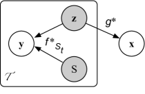
Figure 2: Assumed causal generative model: the gray variables are unobserved. Observations $\mathbf{x}$ are generated by some unknown mixing of a set of factors of variations $\mathbf{z}$. Additionally, we observe a distribution of supervised tasks, only depending on a subset of factors of variations indexed by $S$.

3 Related work

Learning from multiple tasks and domains. Our method addresses the problem of learning a general representation across multiple and possibly unseen tasks [15, 103] and environments [105, 32, 44, 97, 63, 94, 64] that may be competing with each other during training [61, 91, 83]. Prior research tackled task competition by introducing task specific modules that do not interact during training [67, 101, 80]. While successfully learning specialized modules, these approaches can not leverage synergistic information between tasks, when present. On the other hand, our approach is closer to multi-task methods that aim at learning a generalist model, leveraging multi-task interactions [106, 5]. Other approaches that leverage a meta-learning objective for multi-task learning have been formulated [18, 81, 50, 9]. In particular, [50] proposes to learn a generalist model in a few-shot learning setting without explicitly favoring feature sharing, nor sparsity. Instead, we rephrase the multi-task objective function encoding both feature sharing and sparsity to avoid task competition.

Similar to prior work in domain generalization, we assume the existence of stable features for a given task [64, 4, 86, 40, 90] and amortize the learning over the multiple environments. Differently than prior work, we do not aim to learn an invariant representation a priori. Instead, we learn sufficient and minimal features for each task, which are selected at test time fitting the linear head on them. In light of [32], one can interpret our approach as learning the final classifier using empirical risk minimization but over features learned with information from the multiple domains.

Disentangled representations. Disentanglement representation learning [8, 33] aims at recovering the factors of variations underlying a given data distribution. [56] proved that without any form of supervision (whether direct or indirect) on the Factors of Variation (FOV) is not possible to recover them. Much work has then focused on identifiable settings [58, 25] from non-i.i.d. data, even allowing for latent causal relations between the factors. Different approaches can be largely grouped in two categories. First, data may be non-independently sampled, for example assuming sparse interventions or a sparse latent dynamics [30, 55, 13, 100, 2, 79, 48]. Second, data may be non-identically distributed, for example being clustered in annotated groups [37, 41, 82, 95, 60]. Our method follows the latter, but we do not make assumptions on the factor distribution across tasks (only their relevance in terms of sufficiency and minimality). This is also reflected in our method, as we train for supervised classification as opposed to contrastive or unsupervised learning as common in the disentanglement literature. The only exception is the work of [47] discussed in Section 2.3.

4 Experiments

We start by highlighting here the experimental setup of this paper along with its motivation.

Synthetic experiments. We first evaluate our method on benchmarks from the disentanglement literature [62, 14, 71, 49] where we have access to ground-truth annotations and we can assess quantitatively how well we can learn disentangled representations. We further investigate how minimality and feature sharing are correlated with disentanglement measures (Section 4) and how well our representations, which are learned from a limited set of tasks, generalize their composition. The purpose of these experiments is to validate our theoretical statement, showing that if the assumptions of Proposition 2.1 hold, our methods quantitatively recover the factors of variation.

Domain generalization. On real data sets, we can neither quantitatively measure disentanglement nor are we guaranteed identifiability (as assumptions may be violated). Ultimately, the goal of disentangled representations is to learn features that lend themselves to be easily and robustly transferred to downstream tasks. Therefore, we first evaluate the usefulness of our representations with respect to downstream tasks subject to distribution shifts, where isolating spurious features was found to improve generalization in synthetic settings [19, 58] To assess how robust our representations are to distribution shifts, we evaluate our method on domain generalization and domain shift tasks on six different benchmarks (Section 4.2). In a domain generalization setting, we do not have access to samples coming from the testing domain, which is considered to be OOD w.r.t. to the training domains. However, in order to solve a new task, our method relies on a set labeled data at test time to fit the linear head on top of the feature space. Our strategy is to sample data points from the training distribution, balanced by class, assuming that the label set $Y$ does not change in the testing domain, although its distribution may undergo subpopulation shifts.

Few-shot transfer learning. Lastly, we test the adaptability of the feature space to new domains with limited labeled samples. For transfer learning tasks, we fit a linear head using the available limited supervised data. The sparsity penalty $\alpha$ is set to the value used in training; the feature sharing parameter $\beta$ is defaulted to zero unless specified.

Experimental setting. To have a fair comparison with other methods in the literature, we adopt the standard experimental setting of prior work [32, 44]. Hyperparameters $\alpha$ and $\beta$ are tuned performing model selection on validation set, unless specified otherwise. For comparison with baselines, we substitute our backbone with that of the baseline (e.g. for ERM models, we detach the classification head) and then fit a new linear head on the same data. The linear head module trained at test time on top of the features is the same both for our and compared methods. Despite its simplicity, we report the ERM baseline for comparison in our experiments in the main paper, since it has been shown to perform best in average on domain generalization benchmarks [32, 44]. We further compare with other consolidated approaches in the literature such as IRM [4], CORAL [85] and GroupDRO [73] and include a large and comprehensive comparison with [99, 10, 52, 53, 26, 54, 65, 102, 36, 45] in AppendixD.4. Experimental details are fully described in Appendix C.

4.1 Synthetic experiments

We start by demonstrating that our approach is able to recover the factors of variation underlying a synthetic data distribution like [62]. For these experiments, we assume to have partial information on a subset of factors of variation $Z$, and we aim to learn a representation $\hat{\mathbf{z}}$ that aligns with them while ignoring any spurious factors that may be present. We sample random tasks from a distribution $\mathcal{T}$ (see Appendix 5 for details) 5and focus on binary tasks, with $Y=\{0,1\}$. For the DSprites dataset an example of valid task is “There is a big object on the left of the image”. In this case, the partially observed factors (quantized to only two values) are the x position and size. In Table 1, we show how the feature sufficiency and minimality properties enable disentanglement in the learned representations. We train two identical models on a random distribution of sparse tasks defined on FOVs, showing that, for different datasets [62, 14, 49, 71], the same model without regularizers achieves a similar in-distribution (ID) accuracy, but a much lower disentanglement.

\begin{overpic}[width=433.62pt,trim=12.80365pt 0.0pt 31.2982pt 31.2982pt,clip]{pictures/betaVSDCI.png} \put(91.3,57.2){\tiny\cite[cite]{[\@@bibref{Number}{lachapelle2022synergies}{}{}]}} \end{overpic}

Figure 3: Role of minimality: We plot the DCI metric of a set of models (red dots) trained on fixed tasks from DSprites: Training without regularizers leads to no disentanglement (green). Enforcing sparsity alone (yellow, akin to [47]) achieves good disentanglement ($DCI=71.9$), but some features may be split or duplicated. Enforcing both minimality and sparse sufficiency (magenta) attains the best $DCI$ ($98.8$). When $\beta$ is too high ($>0.25$) activated features collapses into few clusters with respect to tasks. For complete results and experiments on additional datasets see Table 8 and Figures 6, 7 in Appendix.

We then randomly draw and fix 2 groups of tasks with supports $S_{1},S_{2}$ (18 in total), which all have support on two FOVs, $|S_{1}|=|S_{2}|=2$. The groups share one factor of variation and differ in the other one, i.e. $S_{1}\cap S_{2}=\{i\}$ for some $\{i\}\in Z$. The data in these tasks are subject to spurious correlations, i.e. FOVs not in the task support may be spuriously correlated with the task label. We start from an overestimate of the dimension of $\tilde{\mathbf{z}}$ of $6$, trying to recover $\mathbf{z}$ of size $3$. We train our network to solve these tasks, enforcing sufficiency and minimality on the representation with different regularization degrees. In Figure 3, we show how the alignment of the learned features with the ground truth factors of variations depend on the choice of $\alpha,\beta$, going from no disentanglement ($DCI=27.8$). to good alignment as we enforce more sufficiency and minimality. The model that attains the best alignment ($DCI=98.8$) uses both sparsity and feature sharing. Sufficiency alone (akin to the method of [47]) is able to select the right support for each task, but features are split or duplicated, attaining lower disentanglement ($DCI=71.9$). The feature sharing penalty ensures clustering in the feature space w.r.t. tasks, ensuring to reach high disentanglement, although it may result in the failure cases, when $\beta$ is too high ($\beta>0.25$).

Table 1: Enforcing disentanglement: DCI [22] disentanglement scores and ID accuracy on test samples for a model trained without enforcing sufficiency and minimality (top row), and model with the regularizers activated (bottom row). While attaining similar performance on accuracy, the model with the activated regularizer always show higher disentanglement. See Table 7 for additional scores.

	Dsprites	3Dshapes	SmallNorb	Cars
No reg
(DCI,Acc)	(16.6,94.4)	(44.4,96.2 )	(16.5,96.1)	(60.5,99.8)
$\alpha,\beta$
(DCI,Acc)	($\mathbf{69.9}$,95.8)	($\mathbf{87.7}$, 95.8)	($\mathbf{55.8}$,95.6 )	($\mathbf{92.3}$,99.8 )

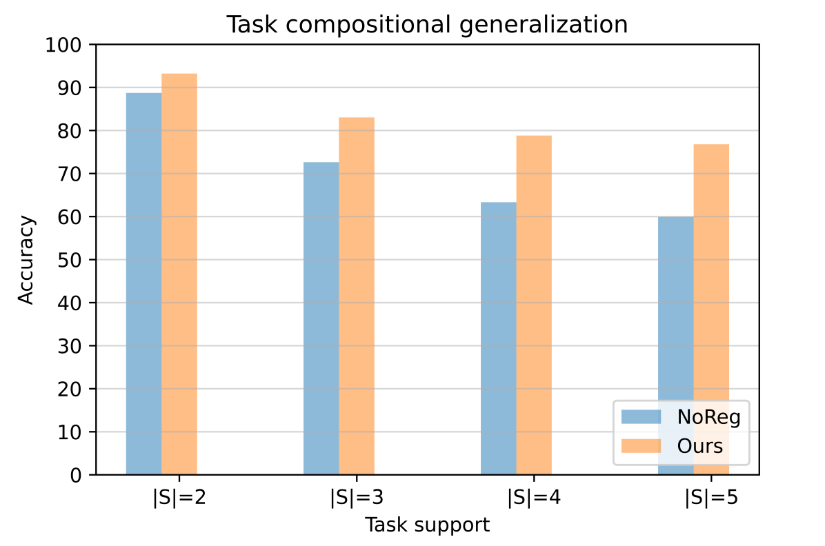
Figure 4: Task compositional generalization: Mean accuracy over 100 random test tasks reported for group of tasks of growing support (second, third, fourth column) for a model trained without inductive biases (blue, attaining $DCI=29.4$) and enforcing them (orange, $DCI=59.4$). The latter show better compositional generalization resulting from the properties enforced on the representation. Exact values are reported in Table 9 in Appendix.

Disentanglement and minimality are correlated. In the synthetic setting, we also show the role of the feature sharing penalty. Minimizing the entropy of feature activations across mini-batches of tasks results in clusters in the feature space. We investigate how the strength of this penalty correlates well with disentanglement metrics [22] training different models on Dsprites which differ by the value of $\beta$. For 15 models trained increasing $\beta$ from $0$ to $0.2$ linearly, we observe a correlation coefficient with the DCI metric associated to representations compute by each model of $94.7$, showing that the feature sharing property strongly encourages disentanglement. This confirms again that sufficiency alone (i.e. enforcing sparsity) is not enough to attain good disentanglement.

Task compositional generalization. Finally, we evaluate the generalization capabilities of the features learned by our method by testing our model on a set of unseen tasks obtained by combining tasks seen during training. To do this, we first train two models on the AbstractDSprites dataset using a random distribution of tasks, where we limit the support of each task to be within 2 (i.e. $|S|=2$). The models differ in activating/deactivating the regularizers on the linear heads. Then, we test on 100 tasks drawn from a distribution with increasing support on the factors of variation $(|S|=3,|S|=4,|S|=5)$, which correspond to composition of tasks in the training distribution; see Figure 4, with the accompaning Table 9 in Appendix D.

4.2 Domain Generalization

Table 2: Quantitative results for few-shot transfer learning, with our method consistently outperforming ERM across all sample sizes and data sets.

N-shot/Algorithm		OOD accuracy (averaged by domains)
1-shot	PACS	VLCS	OfficeHome	Waterbirds
ERM	80.5	$59.7$	56.4	79.8
Ours	$\mathbf{81.5}$	$\mathbf{68.2}$	$\mathbf{58.4}$	$\mathbf{88.4}$
5-shot
ERM	87.1	71.7	75.7	79.8
Ours	$\mathbf{88.3}$	$\mathbf{74.5}$	$\mathbf{77.0}$	$\mathbf{87.6}$
10-shot
ERM	87.9	74.0	81.0	84.2
Ours	$\mathbf{90.4}$	$\mathbf{77.3}$	$\mathbf{82.0}$	$\mathbf{89.2}$

In this section we evaluate our method on benchmarks coming from the domain generalization field [32, 93, 70] and subpopulation distribution shifts [73, 44], to show that a feature space learned with our inductive biases performs well out of real world data distribution.

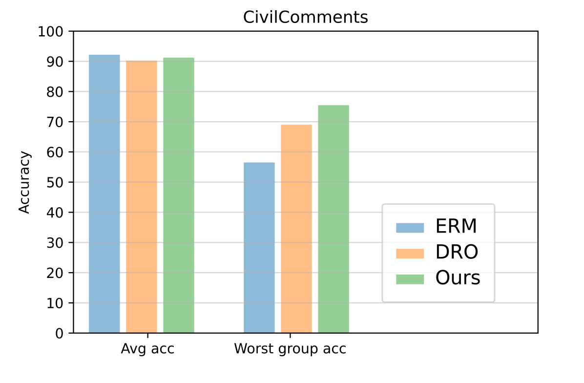
Figure 5: Quantitative results on CivilComments: we report the accuracy on test averaged across all demographic groups (left group), and the worst group accuracy, on the right. Our method (green) performs similarly in terms of average accuracy and outperforms in terms of worst group accuracy, without using any knowledge on the group composition in the training data. For exact values and error estimates, see Table 10 in the Appendix.

Subpopulation shifts.  Subpopulation shifts occur when the distribution of minority groups changes across domains. Our claim is that a feature space that satisfies sparse sufficiency and minimality is more robust to spurious correlations which may affect minority groups, and should transfer better to new distributions. To validate this, we test on two benchmarks Waterbirds [73], and CivilComments [44] (see Appendix C.1).

For both, we use the train and test split of the original dataset. In Table 4, last row, we report the results on the test set of Waterbirds for the different groups in the dataset (landbirds on land, landbirds on water, waterbirds on land, and waterbirds on water, respectively). We fit the linear head on a random subset of the training domain, balanced by class, repeat 10 times and report accuracy and standard deviation on test. For CivilComments we report the average and worst accuracy in Figure 5, where we compare with ERM and groupDRO [73]. While performing almost on par w.r.t. ERM, our method is more robust to spurious correlation in the dataset, showing the higher worst group accuracy. Importantly, we outperform GroupDRO, which uses information on the subdomain statistics, while we do not assume any prior knowledge about them. Results per group are reported in the Appendix (Table 11).

DomainBed. We evaluate the domain generalization performance on the PACS, VLCS and OfficeHome datasets from the DomainBed [32] test suite (see Appendix C.1 for more details). On these datasets, we train on $N-1$ and leave one out for testing. Regularization parameters $\alpha$ and $\beta$ are tuned according to validation sets of PACS, and used accordingly on the other dataset. For these experiments we use a ResNet50 pretrained on Imagenet [17] as a backbone, as done in [32] To fit the linear head we sample 10 times with different samples sizes from the training domains and we report the mean score and standard deviation. Results are reported in Table 4, showing how enforcing sparse sufficiency and minimality leads consistently to better OOD performance. Comparisons with 13 additional baselines is in Appendix D.4.

Table 3: Quantitative evaluation on Camelyon17: we report accuracy both on ID and OOD splits. Our approach achieves significantly higher validation and test OOD accuracy.

	Validation(ID)	Validation (OOD)	Test (OOD)
ERM	93.2	84	70.3
CORAL	$\mathbf{95.4}$	86.2	59.5
IRM	91.6	86.2	64.2
Ours	93.2 ±0.3	$\mathbf{89.9}$±0.6	$\mathbf{74.1}$±0.2

Camelyon17. The model is trained according to the original splits in the dataset. In Table 3 we report the accuracy of our model on in-distribution and OOD splits, compared with different baselines [84, 4]. Our method shows the best performance on the OOD test domains. The intuition of why this happens is that, due to minimality, we retain more features which are shared across the three training domains, giving less importance to the ones that are domain-specific (which contain the spurious correlations with the hospital environmental informations). This can be further enforced at test time, as we show in the ablation in Appendix D.9, trading off in distribution performance for OOD accuracy.

Table 4: Results for domain generalization on DomainBed. Our approach achieves consistently higher average OOD generalization, outperforming ERM in all cases except one.

Dataset/Algorithm		OOD accuracy (by domain)
PACS	S	A	P	C	Average
ERM	77.9 $\pm$ 0.4	$\mathbf{88.1}$ $\pm$ 0.1	97.8 $\pm$ 0.0	79.1 $\pm$ 0.9	85.7
Ours	$\mathbf{83.1}$ $\pm$ 0.1	86.7$\pm$ 0.8	$\mathbf{97.8}$ $\pm$ 0.1	$\mathbf{83.5}$ $\pm$ 0.1	$\mathbf{87.5}$
VLCS	C	L	V	S	Average
ERM	97.6$\pm$ 1.0	63.3 $\pm$ 0.9	76.4 $\pm$ 1.5	72.2 $\pm$ 0.5	77.4
Ours	$\mathbf{98.1}$$\pm$ 0.2	$\mathbf{63.4}$$\pm$ 0.5	$\mathbf{78.2}$ $\pm$ 0.7	$\mathbf{73.9}$$\pm$ 0.8	$\mathbf{78.4}$
OfficeHome	C	A	P	R	Average
ERM	53.4$\pm$ 0.6	62.7 $\pm$ 1.1	76.5 $\pm$ 0.4	77.3 $\pm$ 0.	67.5
Ours	$\mathbf{56.3}$$\pm$ 0.1	$\mathbf{66.7}$ $\pm$ 0.7	$\mathbf{79.2}$$\pm$ 0.5	$\mathbf{81.3}$ $\pm$ 0.4	$\mathbf{70.9}$
Waterbirds	LL	LW	WL	WW	Average
ERM	98.6 $\pm$ 0.3	52.05 $\pm$ 3	68.5 $\pm$ 3	93 $\pm$ 0.3	81.3
Ours	$\mathbf{99.5}$ $\pm$ 0.1	$\mathbf{73.0}$ $\pm$ 2.5	$\mathbf{85.0}$ $\pm$ 2	$\mathbf{95.5}$ $\pm$ 0.4	$\mathbf{90.5}$

4.3 Few-shot transfer learning.

We finally show the ability of features learned with our method to adapt to a new domain with a small number of samples in a few-shot setting. We compare the results with ERM in Table 2, averaged by domains in each benchmark dataset. The full scores for each domain are in Appendix D.5 for 1-shot, 5-shot, and 10-shot setting, reporting the mean accuracy and standard deviations over 100 draws. Our approach achieves consistently higher accuracy than ERM, showing the better adaptation capabilities of our minimal and sufficently sparse feature space.

4.4 Additional results

In Appendix D we report a large collection of additional results, including comparison with 14 baseline methods on the domain shift benchmarks (D.4), a qualitative and quantitative analysis on the minimality and sparse sufficiency properties in the real setting (D.2), a favorable additional comparison on meta learning benchmarks, with 6 other baselines including  [47](D.8), an ablation study on the effect of clustering features at test time (D.9), and a demonstration on the possibility to obtain a task similarity measure as a consequence of our approach (D.7).

5 Conclusions

In this paper, we demonstrated how to learn disentangled representations from a distribution of tasks by enforcing feature sparsity and sharing. We have shown this setting is identifiable and have validated it experimentally in a synthetic and controlled setting. Additionally, we have empirically shown that these representations are beneficial for generalizing out-of-distribution in real-world settings, isolating spurious and domain specific factors that should not be used under distribution shift.

Limitations and future work: The main limitation of our work is the global assumption on the strength of the sparsity and feature sharing regularizers $\alpha$ and $\beta$ across all tasks. In real settings these properties of the representations might need to change for different tasks. We have already observed this in the synthetic setting in Figure 3, where when $\beta>0.25$ features cluster excessively and are unable to achieve clear disentanglement and do not generalize well. Future work may exploit some level of knowledge on the task distribution (e.g. some measure of distance on tasks) in order to tune $\alpha,\beta$ adaptively during training, or to train conditioning on a distribution of regularization parameters as in [21], enabling more generalization at test time. Another limitation is in the sampling procedure to fit the linear head at test time: sampling randomly from the training set (balanced by class) may not be enough to achieve the best performance under distributions shifts. Alternative sampling procedures, e.g. ones that incorporate knowledge on the distribution shift if available (as in [43]), may lead to better performance at test time.

Appendix A Proof of Proposition 1

To prove Proposition 2.1 we rely on the same proof construction of [58], adapting it to our setting. Intuitively, the proposition states that when minimality and sparse sufficiency properties hold it is possible to recover the factors of variations $z$ given enough observations from $p(x,y)$, if the following assumptions on the task distribution hold: (i) the probability of two arbitrary tasks having a singleton intersection of support on the factor of variations is non zero; (ii) the probability that their difference of supports is a singleton is non zero.

The proof is sketched in three steps:

• First, we prove identifiability when the support $S$ of a task is arbitrary but fixed, where we drop the subscript $t$ for convenience.

• Second, we randomize on $S$, to extend the proof for $S$ drawn at random.

• Third, we extend the proof to the case when the dimensionality of $\mathcal{Z}$ is unknown and we start on overestimate of it to recover it.

Identifiability with fixed task support We assume the existence of the generative model in Figure 2, which we report here for convenience:

$$p(\mathbf{z})= \prod_{i}p(z_{i})\ \ \ \ \ \ \ \ \ \ \ \ \ \ \ \ \ S\sim p(S)$$ (6)

$$\mathbf{x}=g^{*}(\mathbf{z}) y=f_{S}^{*}(\mathbf{z})$$ (7)

together with the assumptions specified in theorem statement. We fix the support of the task $S$. We indicate with $g:Z\rightarrow X$ the invertible smooth, candidate function we are going to consider, whose inverse corresponds to $q(\mathbf{z}|\mathbf{x})$. We denote with $T\in S$ which indexes the coordinate subspace of image of $g^{-1}$ corresponding to the unknown coordinate subspace $S$ of factors of variation on which the fixed task depends on. Fixing $T$ requires knowledge of $|S|$. The candidate function $g^{-1}$ must satisfy:

$$f|_{T}(g^{-1}(\mathbf{x}))=y$$ (8)

$$f|_{\bar{T}}(g^{-1}(\mathbf{x}))\neq y$$ (9)

where $\bar{T}$ denotes the indices in the complement of $T$. $f$ denotes a predictor which satisfies the same assumptions on $f^{*}$ on $T$ . We parametrize $g^{-1}$ with $g^{*-1}$ and set:

$g^{-1}=h^{-1}\circ g^{*-1}$ where $h:[0,1]^{d}\rightarrow Z$, mapping from the uniform distribution on $\mathbb{R}^{d}$ to $Z$. We can rewrite the two above constraints as:

$$f|_{T}(h^{-1}(z))=y$$ (10)

$$f|_{\bar{T}}(h^{-1}(z))\neq y$$ (11)

We claim that the only admissible functions $h^{-1}$ maps each entry in $\mathbf{z}$ to unique coordinate in $T$. We observe that due to its smoothness and invertibility, $h^{-1}$ maps $Z$ to the submanifolds $\mathcal{M}_{s},\mathcal{M}_{\bar{s}}$, which are disjoint. By contradiction:

• if $\mathcal{M}_{\bar{S}}$ does not lie in $\bar{T}$ then minimality is violated.

• if $\mathcal{M}_{S}$ does not lie in $T$ then sufficiency is violated

$h^{-1}$ maps each entry in $\mathbf{z}$ to unique coordinate in $T$. Therefore there exist a permutation $\pi$ s.t.:

$$h_{T}^{-1}(\mathbf{z})=\bar{h}_{T}(\mathbf{z}_{\pi(S)})$$ (12)

$$h_{\bar{T}}^{-1}(\mathbf{z})=\bar{h}_{\bar{T}}(\mathbf{z}_{\pi(\bar{S})})$$ (13)

The Jacobian of $h^{-1}$ is a blockwise matrix with block indexed by $T$. So we can identify the two blocks of factors in $S,\bar{S}$ but not necessarily the factors within, as they may be still entangled.

Randomization on $S$

we now consider $S$ to be drawn at random, therefore we observe $p(\mathbf{x},y|S)$ without never observing $S$ directly. $g^{-1}$ must now associate each $p(\mathbf{x},y)$ with a unique $T$, as well as a unique predictor $f$ , for each $S\sim p(S)$ Indeed suppose that $p(\mathbf{x},y|S=S_{1})$ and $p(\mathbf{x},y|S=S_{2})$ with $S_{1},S_{2}\sim p(S)$ and $S_{1}\neq S_{2}$. Then if $T$ would be the same for both tasks (as $f$), eq (6) could only be satisfied for a subset of size $|S_{1}\cap S_{2}|<|S_{1}\cup S_{2}|$ , while $T$ is required to be of size $|S_{1}\cup S_{2}|$ This corresponds to say that each task has its own sparse support and its own predictor. Conversely all $p(\mathbf{x},y)\in supp(p(\mathbf{x},y|S))$ need to be associated to the $T$ and the same predictor $f$, since they will all share the same subspace and cannot be associated to different $T$. Notice also that $|S_{1}\cap S_{2}|=|T_{1}\cap T_{2}|$ and $|S_{1}\cup S_{2}|=|T_{1}\cup T_{2}|$. We further assume:

$\forall z_{i}$ either $p(S\cap S^{\prime}=\{i\})>0$ or $p(\{i\}\in(S\cup S^{\prime})-(S^{\prime}\cap S))>0$

We observe every factor as the intersection of the sets $S,S^{\prime}$ which will be reflected in $T,T^{\prime}$ or we observe single factors in the difference between the intersection and the union of $S,S^{\prime}$. Examples of the two cases are illustrated below:

This together with (8) and (9) implies:

$$h_{i}^{-1}(\mathbf{z})=\bar{h}_{i}(z_{\pi(i)})\ \ \ \ \forall i\in[d]$$ (14)

This further implies that the jacobian of $\bar{h}$ is diagonal. By the change of variable formula we have:

$$q(\mathbf{\hat{z}})=p(\tilde{h}(\mathbf{z}_{\pi([d])}))\left|det\frac{\partial}{\partial\mathbf{z}_{\pi([d]))}}\tilde{h}\right|=\prod_{i01}^{d}p(\tilde{h_{i}}(z_{\pi(i)}))\left|\frac{\partial}{\partial z_{\pi(i)}}\tilde{h}_{i}\right|$$ (15)

This holds for the jacobian being diagonal and invertibility of $\tilde{h}$. Therefore $q(\hat{\mathbf{z}})$ is a coordinate-wise reparametrization of $p(\mathbf{z})$ up to a permutation of the indices. A change in a coordinate of $\mathbf{z}$ implies a change in the unique corresponding coordinate of $\hat{\mathbf{z}}$, so $g$ disentangles the factors of variation.

Dimensionality of the support $S$

Previously we assumed that the dimension of $\hat{\mathbf{z}}$ is the same as $\mathbf{z}$. We demonstrate that even when $d$ is unknown starting from an overstimate of it, we can still recover the factors of variations. Specifically, we consider the case when $\hat{d}>d$. In this case our assumption about the invertibility of $h$ is violated. We must instead ensure that $h$ maps $Z$ to a subspace of $\hat{Z}$ with dimension $d$. To substitute our assumption on inveribility on $h$, we will instead assume that $\mathbf{z}$ and $\hat{\mathbf{z}}$ have the same mutual information with respect to task labels $Y$, i.e.$I(Z,Y)=I(\hat{Z},Y)$ Note that mutual information is invariant to invertible transformation, so this property was also valid in our previous assumption.

Now, consider two arbitrary tasks with $|S\cap S^{\prime}|\neq\emptyset$ =$k$ but $|T\cap T^{\prime}|<k$, i.e. some features are duplicated/splitted. Hence $f,f^{\prime}$ while have different support , i.e.:

$$f|_{T}=f^{\prime}|_{T^{\prime}}=f^{*}$$

We observe that in this situation nor sufficiency, nor minimality are necessarily violated because:

• $f|_{T}=f^{\prime}|_{T^{\prime}}=f^{*}$ (sufficiency is not violated)

• $T\cap T^{\prime}=\emptyset\implies T\not\subset T^{\prime},T^{\prime}\not\subset T$ (minimality is not violated)

In other words we must ensure that a single fov $z_{i}$ is not mapped to different entries in $\hat{\mathbf{z}}$ (feature splitting or duplication). We fix two arbitrary tasks with $|S\cap S^{\prime}|\neq\emptyset$ =$k$ but $|T\cap T^{\prime}|<k$, i.e. some features are duplicated. We know that $|S|=|T|$ and $|S^{\prime}|=|T^{\prime}|$ otherwise sufficency and minimaliy would be violated. Then if $|T\cap T^{\prime}|<k$, then $|T\cup T^{\prime}|>|S\cup S^{\prime}|=d-k$ we have $p(|T\cup T^{\prime}|)$=$p(supp(p(y|\hat{\mathbf{z}}))+supp(p^{\prime}(y^{\prime}|\hat{\mathbf{z^{\prime}}})))=p(\sum_{i}supp(f_{i}(.))$ , and since

$$H[p(\sum_{i}supp(f_{i}(.))]>H[p(\sum_{i}supp(f_{i}(.))]$$ (16)

but we have assumed:

$$I(Z,Y) =I(\hat{Z},Y)$$ (17)

$$\cancel{H(Y)}-H(Y|\hat{Z}) =\cancel{H(Y)}-H(Y|Z)$$ (18)

$$H(Y|\hat{Z}) =H(Y|Z)$$ (19)

$$H[p(Y|\hat{Z})>0] =H[p(Y|Z)>0]$$ (20)

$$2^{H[p(Y|\hat{Z})>0]} =2^{H[p(Y|Z)>0]}$$ (21)

$$|supp(p(Y|\hat{Z}))| =|supp(p(Y|Z)|$$ (22)

this last passage is due to relation between cardinality and entropy: for uniform distributions the exponential of the entropy is equal to the cardinality of the support of the distribution.

$$|supp(f)|=|supp(f^{*})|$$ (23)

We know that (12) must hold for every task, therefore: $\sum_{i}I(Z,Y_{i})=\sum_{i}I(\hat{Z},Y_{i})$ for each $i$ then: $\sum_{i}|supp(\hat{f_{i}})|=\sum_{i}|supp(f_{i}^{*})|$ $|\bigcup_{i}T_{i}|=|\bigcup_{i}S_{i}|$ therefore (12) contradicts our assumption (13).

Appendix B Implementation details

B.1 Training algorithm

Algorithm 1 Training algorithm

1:  Input: A task distribution $\mathcal{T}$

2:  while Not converged do

3:     Sample a batch $B_{T}$ of $T$ tasks $t\sim\mathcal{T}$

4:     Sample $(U_{t},Q_{t})$ from each task in the batch

5:     $\#$ Inner loop

6:     for each $t$ in $B_{T}$ do

7:        Compute $\mathbf{z}_{t}^{U}=g_{\theta}(\mathbf{x}_{t}^{U})$

8:     end for

9:     Solve $\phi^{*}=argmin_{\phi}\frac{1}{T}\sum_{t}\mathcal{L}_{inner}(f_{\phi}(\mathbf{z}_{t}^{U}),y_{t}^{U})+Reg(\phi)$

10:     $\#$ Outer loop

11:     for each $t$ do

12:        Compute $\mathbf{z}_{t}^{Q}=g_{\theta}(\mathbf{x}_{t}^{Q})$

13:     end for

14:     Compute $\mathcal{L}_{outer}(f_{\phi^{*}}(g_{\theta}(\mathbf{x}_{t}^{Q}),y_{t}^{Q}))$

15:     Compute $\frac{\partial\mathcal{L}_{outer}(\theta)}{\partial\theta}$ as in [28]

16:     Update $\theta$

17:  end while

B.2 Implicit gradients

In the backward pass, denoting with $\mathcal{L}_{outer}^{*}=\mathcal{L}_{outer}(f_{\phi}^{*}(g_{\theta}(x^{Q})),Y^{Q})$ denoting the loss computed with respect to the optimal classifier $f_{\phi}^{*}$ on the query samples $(x^{Q},Y^{Q})$, we have to compute the following gradient:

$$\frac{\partial\mathcal{L}_{outer}^{*}(\theta)}{\partial\theta}=\frac{\partial\mathcal{L}_{outer}(\theta,\phi^{*})}{\partial\theta}+\frac{\mathcal{L}_{outer}(\theta,\phi^{*})}{\partial{\phi^{*}}}\frac{\partial\phi^{*}}{\partial\theta}$$ (24)

where is the algorithm procedure to solve Eq1, i.e. SGD. While is just the gradient of the loss evaluated at the solution of the inner problem and can be computed efficiently with standard automatic backpropagation, requires further attention. Since the solution to $C_{\phi^{*}}$ is implemented via and iterative method (SGD), one strategy would be to compute this gradient would be to backpropagate trough the entire optimization trajectory in the inner loop. This strategy however is computational inefficient for many steps, and can suffer also from vanishing gradient problems.

Appendix C Experimental details

All experiments were performed on a single gpu NVIDIA RTX 3080Ti and implemented with the Pytorch library [69].

C.1 Datasets

We evaluate our method on a synthetic setting on the following benchmarks: DSprites, AbstractDSprites[62], 3Dshapes [14],SmallNorb [49], Cars3D[71] and the semi-synthetic Waterbirds [73].

For domain generalization and domain adaptation tasks, we evaluate our method on the [32] and [44] benchmarks, using the following datasets: PACS[51], VLCS[3], OfficeHome[87] Camelyon17[6], CivilComments [12].

Dataset descriptions

The Waterbirds dataset [73] is a synthetic dataset where images are composed of cropping out birds from photos in the Caltech-UCSD Birds-200-2011 (CUB) dataset [89] and transferring them onto backgrounds from the Places dataset [104]. The dataset contains a large percentage of training samples ($\approx\%95$) which are spuriously correlated with the background information.

The CivilComments is a dataset of textual reviews annotated with demographics information for the task of detecting toxic comments. Prior work has shown that toxicity classifiers can pick up on biases in the training data and spuriously associate toxicity with the mention of certain demographics [68, 20]. These types of spurious correlations can significantly degrade model performance on particular subpopulations [74].

The PACS dataset [51] is a collection of images coming from four different domains: real images, art paintings, cartoon and sketch. The VLCS dataset contains examples from 5 overlapping classes from the VOC2007 [23], LabelMe [72], Caltech-101 [24] , and SUN [98] datasets. The OfficeHome dataset contains 4 domains (Art, ClipArt, Product, real-world) where each domain consists of 65 categories.

The Camelyon17 dataset, is a collection of medical tissue patches scanned from different hospital environments. The task is to predict whether a patch contain a benign or tumoral tissue. The different hospitals represent the different domains in this problem, and the aim is to learn a predictor which is robust to changes in factors of variation across different hospitals.

C.2 Models

For synthetic datasets we use a CNN module for the backbone $g\theta$ following the architecture in Table 5. For real datasets that use images as modality we use a ResNet50 architecure as backbone pretrained on the Imagenet dataset. For the experiments on the text modality we use DistilBERT model [76] with pretrained weights downloaded from HuggingFace [96].

C.3 Synthetic experiments

Table 5: Convolutional architecture used in synthetic experiments.

CNN backbone
Input : $64\times 64\times$ number of channels
$4\times 4$conv, $32$ stride $2$, padding $1$, ReLU,BN
$4\times 4$conv, $32$ stride $2$, padding $1$, ReLU,BN
$4\times 4$conv, $64$ stride $2$, padding $1$, ReLU,BN
$4\times 4$conv, $64$ stride $2$, padding $1$, ReLU,BN
FC, $256$, Tanh
FC, $d$

Task generation. For the synthetic experiments we have access to the ground truth factors of variations $\mathcal{Z}$ for each dataset. The task generation procedure relies on two hyperparameters: the first one is an index set $\mathbb{S}$ of possible factors of variations on which the distribution of tasks can depend on. The latter hyperparameter $K$, set the maximum number of factors of variations on which a single task can depend on. Then a task $t$ is sampled drawing a number $k_{t}$ from $\{1...K\}$, and then sampling randomly a subset $S$ of size $|\mathbb{S}|-k_{t}$ from $\mathbb{S}$. The resulting set $S$ will be the set indexing the factors of variation in Z on which the task $t$ is defined. In this setting restrict ourselves to binary task: for each factors in $S$, we sample a random value $v$ for it. The resulting set of values $V$, will determine uniquely the binary task.

Before selecting $v\in V$ we quantize the possible choices corresponding to factors of variations which may have more than six values to 2. We remark that this quantization affect only the task label definition. For examples for x axis factor, we consider the object to be on the left if its x coordinate is less than the medial axis of the image, on the right otherwise. The DSprites dataset has the following set of factors of variations $Z_{dsprites}=\{shape,size,angle,x_{pos},y_{pos}\}$ and example of task is There is a big object on the right where $k_{t}=2$ the affected factors are $size,x_{pos}$. Another example is There is a small heart on the top left , where $k_{t}=4$ the affected factors are $shape,size,x_{pos},y_{pos}$. Obervations are labelled positively of negatively if their corresponding factors of variations matching in the values with the one specified by the current task.

We then samples random query $Q$ and support $U$ set of samples balanced with respect to postive and negative labels of task task $t$, using stratified sampling.

C.4 Experiments on domain shifts

For the domain generalization and few-shot transfer learning experiments we put ourselves in the same settings of [32, 44] to ensure a fair comparison. Namely, for each dataset we use the same augmentations, and same backbone models.

For solving the inner problem in Equation 5, we used Adam optimizer [42], with a learning rate of $1e-2$, momentum $0.99$, with the number of gradient steps varying from $50$ to $100$, in domain shifts experiments.

Task generation. The task (or episode) sampling procedure is done as follows: each task is a multiclass classification problem: we set the number of classes $C$ to $C=5$ when the original number of classes $K_{train}$ in the dataset is higher than five, i.e. $K_{train}>5$. Otherwise we set $C=K_{train}$. During training, the sizes of the support set $U$ and query sets $Q$ where set to $|U|=25,|Q|=15$ similar to as done in prior meta-learning literature [50, 18]. Changing these parameters has similar effects from what has been observed in many meta learning approaches(e.g. [50, 18]).

For binary datasets such as Camelyon17 or Waterbirds the possible classes to be predicted are always the same across tasks: what is changing is the composition of $U$ and $Q$. Keeping their cardinality low, we ensure that some tasks will not contain spurious correlation that may be present in the dataset, while other ones will still retain it, and the regularizers will satisfy solutions which discards the spurious information. We can observe evidence of this in the experimental results in Tables 3, 4 and qualitatively in Figure 8.

C.5 Selection of $\alpha$ and $\beta$

To find the best regularization parameters $\alpha,\beta$ weighting the sparsity and feature sharing regularizers in Equation 1 respectively, we perform model selection according to the highest accuracy on a validation set. We report in Table 6 the value selected for each experiment.

Table 6: Selected values for $\alpha$ and $\beta$ for all experiments, applying model selection on validation set.

Experiment	$\mathbf{\alpha}$	$\mathbf{\beta}$
Table 1	1e-2	0.15
Table 2	1e-2	5e-2
Table 3	2.5e-3	5e-2
Table 4	1.5e-3	1e-2
Table 5, 6	2.5e-3	1e-2
Table 7	2.5e-3	1e-2

Appendix D Additional results

D.1 Synthetic experiments

Enforcing disentanglement: In Table 7 we report diverse disentanglement scores (DCI disentanglement, DCI completeness, DCI informativeness) on the DSprites, 3DShapes, SmallNorb,Cars datasets, showing that the sparsity and feature sharing regularizers effectively enforce disentanglement.

Table 7: Enforcing disentanglement. DCI [22] disentanglement, completeness and informativeness scores and ID accuracy on test samples for a model trained without enforcing sufficiency and minimality (top row), and model with the regularizers activated (bottom row). While attaining similar performance on accuracy, the model with the activated regularizer always show higher disentanglement. See Table for additional scores.

	DSprites	3DShapes	SmallNorb	Cars
Without regularization
DCI Disentanglement	16.6	44.4	16.5	60.5
DCI Completeness	17.5	39.1	12.9	50.8
DCI Informativeness	88.0	87.6	90.5	95.5
With regularization
DCI Disentanglement	69.9	87.7	60.5	92.3
DCI Completeness	72.3	88.4	63.2	57.1
DCI Informativeness	96.0	95.7	95.4	99.7

\begin{overpic}[width=260.17464pt,trim=12.80365pt 0.0pt 31.2982pt 31.2982pt,clip]{pictures/betaVSDCI3dshapes.png} \put(26.3,16.0){ \tiny{\cite[cite]{[\@@bibref{Number}{lachapelle2022synergies}{}{}]}}} \end{overpic}

Figure 6: Role of minimality (3DShapes): We plot the DCI disentanglement metric of a set of models (red dots) trained on fixed tasks from 3Dshapes: Training without regularizers leads to no disentanglement (green). Enforcing sparsity alone (yellow, akin to [47]) achieves good disentanglement ($DCI=67.0$), but some features may be split or duplicated. Enforcing both minimality and sparse sufficiency (magenta) attains the best $DCI$ ($95.9$). When $\beta$ is too high ($>0.25$) activated features collapses into few clusters with respect to tasks.

The role of minimality. In Figure 7 we show the qualitative results accompanying Figure 3. The qualitative results in the Figure are produced visualizing matrices of feature importance [57] computed fitting Gradient Boosted Trees (GBT) on the learned representations w.r.t. task labels, and on the factors of variations w.r.t. task labels and compare the results. In each matrix the x axis represents the tasks and the y axis the features, and each entries the amount of feature importance (which goes from 0 to 1). In Figure 6 we show the same experiment on the 3DShapes dataset.

Task compositional generalization. In Table 9 we show the quantitative results accompanying Figure 4.

\begin{overpic}[width=303.53267pt,trim=284.52756pt 79.6678pt 256.0748pt 56.9055pt,clip]{pictures/featuresharing.png} \put(15.0,15.0){\tiny$\beta=0.4,DCI=30.5$ } \put(10.0,36.0){\tiny$\beta=0,\alpha=0,DCI=27.8$ } \put(15.0,54.0){\tiny$\beta=0,DCI=71.9$ } \put(15.0,71.0){\tiny$\beta=0.2,DCI=98.8$ } \end{overpic}

Figure 7: Qualitative dependency of disentanglement from the weight of our penalties ($\alpha=0.01$ unless otherwise specified). The model that attains the best disentanglement ($DCI=98.8$) uses both. Left column, top: ground-truth importance weights of each latent factor for each task. Right column: we train models with different $\beta$ and visualize the weights assigned to each learned feature on each task. Left column: to determine whether the model recover the ground-truth latents, we select the 3 top features and compare their assigned weights on different tasks with the ground-truth weights. Bottom row: example of a failure case with high $\beta$.

Table 8: Quantitative results accompanying Figure 7

	$\alpha=0,\beta=0$	$\alpha=1e-2,\beta=0$	$\alpha=1e-2,\beta=0.2$	$\alpha=1e-2,\beta=0.4$
DCI	27.8	71.9	98.8	30.5

Table 9: Task compositional generalization: Mean accuracy over 100 random tasks reported for group of tasks of growing support (second, third, fourth column) for a model trained without inductive biases (top row) and enforcing them (bottom row). The latter show better compositional generalization resulting from the properties enforced on the representation

	Acc ID	DCI	$|S|=3$	$|S|=4$	$|S|=5$
No reg	88.7	22.8	72.6	63.3	59.9
$\alpha,\beta$	$\mathbf{93.2}$	$\mathbf{59.4}$	$\mathbf{83.0}$	$\mathbf{78.8}$	$\mathbf{76.8}$

D.2 Properties of the learned representations

Feature sufficiency. The sufficiency property is crucial for robustness to spurious correlations in the data. If the model can learn and select the relevant features for a task, while ignoring the spurious ones, sufficiency is satisfied, resulting in robust performance under subpopulation shifts, as shown in Tables 10 and 4. To get qualitative evidence of the sufficiency in the representations, in Figure 8 we show the saliency maps computed from the activations of our model and a corresponding model trained with ERM. Our model can learn features specific to the subject of the image, which are relevant for classification, while ignoring background information. This can be observed in both correctly classified (bottom row) and misclassified (top row) samples by ERM. In contrast, ERM activates features in the background and relies on them for prediction.

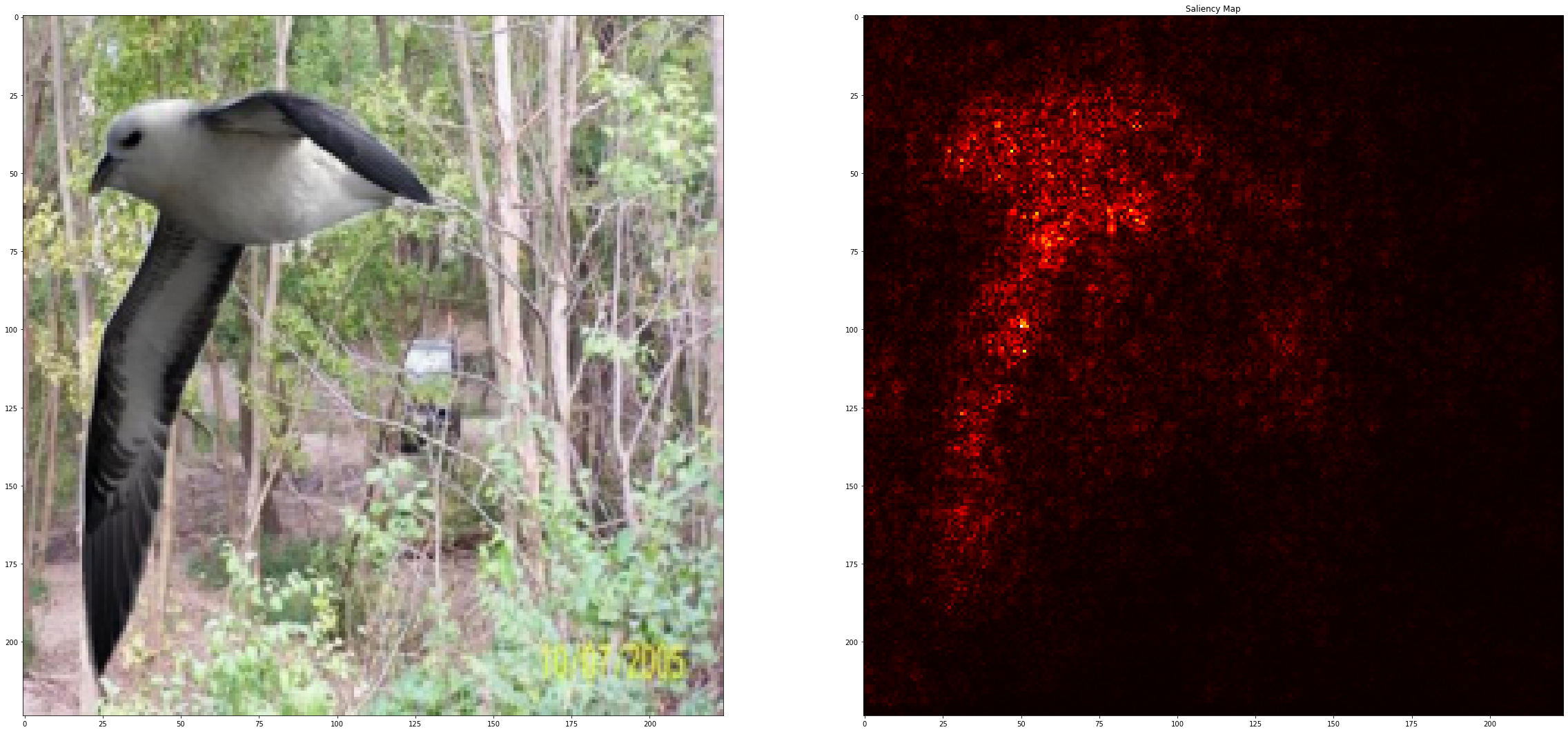
Figure 8: Feature sufficiency: Left, pairs of random samples and saliency maps computed on activations with our method. All samples are correctly classified. Right, corresponding saliency maps [1] an ERM based method: the first row is misclassifed by the network, the last is correctly classified. The ERM model depends on features from the background, resulting in a higher prediction error on mixed subdomains. Our model is robust to spurious correlations and satisfies the sufficiency assumptions.

Feature sharing. In this section, we study the minimality properties of the representations learned by our method. To achieve this, we conduct the following experiment. We randomly draw 14 tasks from the $\sum_{i=1}^{3}\binom{4}{i}$ possible combinations of the four domains in the PACS dataset. We use the data from these tasks to fit the linear head and test the model accuracy on the OOD domain (e.g. the sketch domain). In Figure 9, we show the performance on each task, ordered on the x axis according to OOD accuracy of a model trained with ERM (in yellow). We also report the fraction of activated features (in blue) shared between each task and the OOD task, and the same(red) for the ERM model. The fraction of activated features is computed by looking at the matrix of coefficients of the sparse linear head $\phi\in\mathbb{R}^{M\times C}$, where $M$ is the number of features and $C$ the number of classes, after fitting on each task. Specifically, is computed as $\frac{\sum_{m}\left[\tilde{\phi}_{\epsilon}\cap\tilde{\phi}_{\epsilon}^{OOD}\right]}{\sum_{m}\left[\tilde{\phi}_{\epsilon}\cup\tilde{\phi}_{\epsilon}^{OOD}\right]}$ where $\tilde{\phi}_{\epsilon}=\frac{1}{C}\sum_{c}|\phi_{m,c}|>\epsilon$ and $\phi^{OOD}$ is the matrix of coefficient of the OOD task. We set $\epsilon=0.01$. From Figures 9 and 10 we draw the following conclusions: (i) When the accuracy of the ERM decreases (i.e., the current task is farther from the OOD test task), our method is still able to retain a high and consistent accuracy, demonstrating that our features are more robust out-of-distribution. This is further supported by the higher number of shared features compared to ERM, as we move away from the testing domain. (ii) The correlation between the fraction of shared features and the accuracy OOD demonstrates that the method is able to learn general features that transfer well to unseen domains, thanks to the minimality constraint. Additionally, this measure serves as a reliable indicator of task distance, as discussed in the next section. (iii) Even though the same sparse linear head is used on top of the ERM and our features, our method is able to achieve better OOD performance with fewer features, further demonstrating our feature minimality.

Figure 9: Fraction of shared features VS accuracy. Barplot of OOD accuracies on the Sketch domain for our model (green) and ERM (yellow) on the 14 tasks sampled from PACS, along with the fraction of shared features with the OOD domain for each task (blue for our model, red for ERM). Each task is sampled from a single domain or from the intersections of domains. Tasks are labelled according to the sampling domain on the x axis. The fraction of shared features and OOD accuracy have a correlation coefficient of $97.5$.

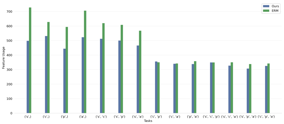
Figure 10: Barplot of feature usage (number of activated features) for each task for our model (blue) and ERM model (green) referring to the experiment in Figure 9. Our method uses fewer features than ERM while also generalizing better.

D.3 CivilComments

See Table 10 for the quantitative results accompanying to Figure 5 in the paper and 11 for result on groups on the civil comments dataset.

Table 10: Quantitative results on CivilComments: we report the accuracy on test averaged across all demographic groups (left), and the worst group accuracy (right). We show that our method performs similarly in terms of average accuracy and outperforms in terms of worst group accuracy, without using any knowledge on the group composition in the training data. This Table accompanies Figure 5

	avg acc	worst group acc
ERM	$\mathbf{92.2}$	56.5
DRO	90.2	69
Ours	91.2 $\pm$ 0.2	$\mathbf{75.45}$$\pm$ 0.1

Table 11: Civilcomments quantitative results pergroup.

	Male	Female	LGBTQ	Christian	Muslim	Other religion	Black	White
GroupDRO
Toxic	$75.1\footnotesize\pm 2.1$	$73.7\footnotesize\pm 1.5$	$73.7\footnotesize\pm 4$	$69.2\footnotesize\pm 2.0$	$72.1\footnotesize\pm 2.6$	$72.0\footnotesize\pm 2.5$	$79.6\footnotesize\pm 2.2$	$78.8\footnotesize\pm 1.7$
Non Toxic	$88.4\footnotesize\pm 0.7$	$90.0\footnotesize\pm 0.6$	$76.0\footnotesize\pm 3.6$	$92.6\footnotesize\pm 0.6$	$80.7\footnotesize\pm 1.9$	$87.4\footnotesize\pm 0.9$	$72.2\footnotesize\pm 2.3$	$73.4\footnotesize\pm 1.4$
Ours
Toxic	$87.94\footnotesize\pm 0.07$	$89.17\footnotesize\pm 0.05$	$77.25\footnotesize\pm 0.16$	$92.25\footnotesize\pm 0.16$	$80.6\footnotesize\pm 0.29$	$87.79\footnotesize\pm 0.26$	$75.45\footnotesize\pm 0.17$	$78.35\footnotesize\pm 0.02$
Non toxic	$91.62\footnotesize\pm 0.11$	$91.52\footnotesize\pm 0.11$	$91.71\footnotesize\pm 0.16$	$91.11\footnotesize\pm 0.1$	$91.81\footnotesize\pm 0.12$	$91.32\footnotesize\pm 0.1$	$90.82\footnotesize\pm 0.12$	$92.04\footnotesize\pm 0.11$

D.4 Full results Domain generalization

We report here comparison with several methods in the domain generalization literature, namely [99, 10, 52, 53, 26, 54, 65, 102, 36, 45].

D.4.1 VLCS

Algorithm	C	L	S	V	Avg
ERM	97.7 $\pm$ 0.4	64.3 $\pm$ 0.9	73.4 $\pm$ 0.5	74.6 $\pm$ 1.3	77.5
IRM	98.6 $\pm$ 0.1	64.9 $\pm$ 0.9	73.4 $\pm$ 0.6	77.3 $\pm$ 0.9	78.5
GroupDRO	97.3 $\pm$ 0.3	63.4 $\pm$ 0.9	69.5 $\pm$ 0.8	76.7 $\pm$ 0.7	76.7
Mixup	98.3 $\pm$ 0.6	64.8 $\pm$ 1.0	72.1 $\pm$ 0.5	74.3 $\pm$ 0.8	77.4
MLDG	97.4 $\pm$ 0.2	65.2 $\pm$ 0.7	71.0 $\pm$ 1.4	75.3 $\pm$ 1.0	77.2
CORAL	98.3 $\pm$ 0.1	66.1 $\pm$ 1.2	73.4 $\pm$ 0.3	77.5 $\pm$ 1.2	78.8
MMD	97.7 $\pm$ 0.1	64.0 $\pm$ 1.1	72.8 $\pm$ 0.2	75.3 $\pm$ 3.3	77.5
DANN	99.0 $\pm$ 0.3	65.1 $\pm$ 1.4	73.1 $\pm$ 0.3	77.2 $\pm$ 0.6	78.6
CDANN	97.1 $\pm$ 0.3	65.1 $\pm$ 1.2	70.7 $\pm$ 0.8	77.1 $\pm$ 1.5	77.5
MTL	97.8 $\pm$ 0.4	64.3 $\pm$ 0.3	71.5 $\pm$ 0.7	75.3 $\pm$ 1.7	77.2
SagNet	97.9 $\pm$ 0.4	64.5 $\pm$ 0.5	71.4 $\pm$ 1.3	77.5 $\pm$ 0.5	77.8
ARM	98.7 $\pm$ 0.2	63.6 $\pm$ 0.7	71.3 $\pm$ 1.2	76.7 $\pm$ 0.6	77.6
VREx	98.4 $\pm$ 0.3	64.4 $\pm$ 1.4	74.1 $\pm$ 0.4	76.2 $\pm$ 1.3	78.3
RSC	97.9 $\pm$ 0.1	62.5 $\pm$ 0.7	72.3 $\pm$ 1.2	75.6 $\pm$ 0.8	77.1
Ours	98.1$\pm$ 0.2	63.4$\pm$ 0.5	73.9 $\pm$ 0.8	78.2 $\pm$ 0.7	78.4

D.4.2 PACS

Algorithm	A	C	P	S	Avg
ERM	84.7 $\pm$ 0.4	80.8 $\pm$ 0.6	97.2 $\pm$ 0.3	79.3 $\pm$ 1.0	85.5
IRM	84.8 $\pm$ 1.3	76.4 $\pm$ 1.1	96.7 $\pm$ 0.6	76.1 $\pm$ 1.0	83.5
GroupDRO	83.5 $\pm$ 0.9	79.1 $\pm$ 0.6	96.7 $\pm$ 0.3	78.3 $\pm$ 2.0	84.4
Mixup	86.1 $\pm$ 0.5	78.9 $\pm$ 0.8	97.6 $\pm$ 0.1	75.8 $\pm$ 1.8	84.6
MLDG	85.5 $\pm$ 1.4	80.1 $\pm$ 1.7	97.4 $\pm$ 0.3	76.6 $\pm$ 1.1	84.9
CORAL	88.3 $\pm$ 0.2	80.0 $\pm$ 0.5	97.5 $\pm$ 0.3	78.8 $\pm$ 1.3	86.2
MMD	86.1 $\pm$ 1.4	79.4 $\pm$ 0.9	96.6 $\pm$ 0.2	76.5 $\pm$ 0.5	84.6
DANN	86.4 $\pm$ 0.8	77.4 $\pm$ 0.8	97.3 $\pm$ 0.4	73.5 $\pm$ 2.3	83.6
CDANN	84.6 $\pm$ 1.8	75.5 $\pm$ 0.9	96.8 $\pm$ 0.3	73.5 $\pm$ 0.6	82.6
MTL	87.5 $\pm$ 0.8	77.1 $\pm$ 0.5	96.4 $\pm$ 0.8	77.3 $\pm$ 1.8	84.6
SagNet	87.4 $\pm$ 1.0	80.7 $\pm$ 0.6	97.1 $\pm$ 0.1	80.0 $\pm$ 0.4	86.3
ARM	86.8 $\pm$ 0.6	76.8 $\pm$ 0.5	97.4 $\pm$ 0.3	79.3 $\pm$ 1.2	85.1
VREx	86.0 $\pm$ 1.6	79.1 $\pm$ 0.6	96.9 $\pm$ 0.5	77.7 $\pm$ 1.7	84.9
RSC	85.4 $\pm$ 0.8	79.7 $\pm$ 1.8	97.6 $\pm$ 0.3	78.2 $\pm$ 1.2	85.2
Ours	86.7 $\pm$ 0.1	83.5 $\pm$ 0.8	97.8 $\pm$ 0.1	83.1 $\pm$ 0.1	87.5

D.4.3 OfficeHome

Algorithm	A	C	P	R	Avg
ERM	61.3 $\pm$ 0.7	52.4 $\pm$ 0.3	75.8 $\pm$ 0.1	76.6 $\pm$ 0.3	66.5
IRM	58.9 $\pm$ 2.3	52.2 $\pm$ 1.6	72.1 $\pm$ 2.9	74.0 $\pm$ 2.5	64.3
GroupDRO	60.4 $\pm$ 0.7	52.7 $\pm$ 1.0	75.0 $\pm$ 0.7	76.0 $\pm$ 0.7	66.0
Mixup	62.4 $\pm$ 0.8	54.8 $\pm$ 0.6	76.9 $\pm$ 0.3	78.3 $\pm$ 0.2	68.1
MLDG	61.5 $\pm$ 0.9	53.2 $\pm$ 0.6	75.0 $\pm$ 1.2	77.5 $\pm$ 0.4	66.8
CORAL	65.3 $\pm$ 0.4	54.4 $\pm$ 0.5	76.5 $\pm$ 0.1	78.4 $\pm$ 0.5	68.7
MMD	60.4 $\pm$ 0.2	53.3 $\pm$ 0.3	74.3 $\pm$ 0.1	77.4 $\pm$ 0.6	66.3
DANN	59.9 $\pm$ 1.3	53.0 $\pm$ 0.3	73.6 $\pm$ 0.7	76.9 $\pm$ 0.5	65.9
CDANN	61.5 $\pm$ 1.4	50.4 $\pm$ 2.4	74.4 $\pm$ 0.9	76.6 $\pm$ 0.8	65.8
MTL	61.5 $\pm$ 0.7	52.4 $\pm$ 0.6	74.9 $\pm$ 0.4	76.8 $\pm$ 0.4	66.4
SagNet	63.4 $\pm$ 0.2	54.8 $\pm$ 0.4	75.8 $\pm$ 0.4	78.3 $\pm$ 0.3	68.1
ARM	58.9 $\pm$ 0.8	51.0 $\pm$ 0.5	74.1 $\pm$ 0.1	75.2 $\pm$ 0.3	64.8
VREx	60.7 $\pm$ 0.9	53.0 $\pm$ 0.9	75.3 $\pm$ 0.1	76.6 $\pm$ 0.5	66.4
RSC	60.7 $\pm$ 1.4	51.4 $\pm$ 0.3	74.8 $\pm$ 1.1	75.1 $\pm$ 1.3	65.5
Ours	66.7 $\pm$ 0.1	56.3 $\pm$ 0.7	79.2 $\pm$ 0.5	81.3 $\pm$ 0.4	70.9

D.5 Few-shot transfer learning

Results on few-shot transfer learning on datasets PACS,VLCS,OfficeHome,Waterbirds in Tables 12,13,14 and 15.

Table 12: Results few-shot transfer learning on PACS

Dataset/Algorithm		OOD accuracy (by domain)
PACS 1-shot	S	A	P	C	Average
ERM	72.3 $\pm$ 0.3	$80.4$ $\pm$ 0.09	93.3 $\pm$ 4.1	75.8$\pm$ 2.6	80.5
Ours	$\mathbf{75.4}$ $\pm$ 3	$\mathbf{81.7}$$\pm$ 0.8	$\mathbf{98.0}$ $\pm$ 0.8	$\mathbf{71}$ $\pm$ 5.2	$\mathbf{81.5}$
PACS 5-shot	S	P	A	C	Average
ERM	84.9$\pm$ 1.1	85.7 $\pm$ 0.08	98.6 $\pm$ 0.0	79.1 $\pm$ 0.9	87.1
Ours	$\mathbf{85.0}$ $\pm$ 0.1	$\mathbf{86.7}$$\pm$ 0.8	$\mathbf{97.8}$ $\pm$ 0.1	$\mathbf{83.5}$ $\pm$ 0.1	$\mathbf{88.3}$
PACS 10-shot	S	P	A	C	Average
ERM	81.0 $\pm$ 0.1	88.9 $\pm$ 0.1	97.4 $\pm$ 0.0	84.2 $\pm$ 0.9	87.9
Ours	$\mathbf{86.2}$ $\pm$ 0.5	$\mathbf{90.0}$ $\pm$ 0.8	$\mathbf{98.9}$ $\pm$ 0.1	$\mathbf{86.6}$ $\pm$ 0.1	$\mathbf{90.4}$

Table 13: results few-shot transfer learning on VLCS

Dataset/Algorithm		OOD accuracy (by domain)
VLCS 1-shot	C	L	V	S	Average
ERM	98.9 $\pm$ 0.4	32.7 $\pm$ 16.2	59.8 $\pm$ 10.7	47.5 $\pm$ 11.2	59.7
Ours	$\mathbf{98.6}$ $\pm$ 0.3	$\mathbf{51.0}$ $\pm$ 4.9	$\mathbf{61.2}$ $\pm$ 9.8	$\mathbf{61.9}$ $\pm$ 9.7	$\mathbf{68.2}$
VLCS 5-shot	C	L	V	S	Average
ERM	99.4 $\pm$ 0.2	50.0 $\pm$ 6.2	71.9 $\pm$ 3.2	65.3 $\pm$ 2.8	71.7
Ours	$\mathbf{98.9}$ $\pm$ 0.4	$\mathbf{56.0}$ $\pm$ 6.2	$\mathbf{73.4}$ $\pm$ 1.4	$\mathbf{69.8}$ $\pm$ 2.0	$\mathbf{74.5}$
VLCS 10-shot	C	L	V	S	Average
ERM	99.5 $\pm$ 0.2	52.6 $\pm$ 5.0	74.8 $\pm$ 3.8	69.1 $\pm$ 2.4	74.0
Ours	$\mathbf{99.1}$ $\pm$ 0.2	$\mathbf{65.0}$ $\pm$ 6.2	$\mathbf{74.4}$ $\pm$ 1.9	$\mathbf{70.8}$ $\pm$ 2.3	$\mathbf{77.3}$

Table 14: results few-shot transfer learning on OfficeHome

Dataset/Algorithm		OOD accuracy (by domain)
OfficeHome 1-shot	C	A	P	R	Average
ERM	40.2 $\pm$ 2.4	52.7 $\pm$ 2.6	68.1 $\pm$ 1.7	64.6 $\pm$ 1.8	56.4
Ours	$\mathbf{41.4}$ $\pm$ 1.7	$\mathbf{54.5}$ $\pm$ 2.0	$\mathbf{68.5}$ $\pm$ 2.7	$\mathbf{69.0}$ $\pm$ 1.5	$\mathbf{58.4}$
OfficeHome 5-shot	C	A	P	R	Average
ERM	63.2 $\pm$ 0.4	73.3 $\pm$ 0.8	84.1 $\pm$ 0.4	82.0 $\pm$ 0.8	75.7
Ours	$\mathbf{66.2}$ $\pm$ 1.2	$\mathbf{75.1}$ $\pm$ 1.0	$\mathbf{83.6}$ $\pm$ 0.5	$\mathbf{83.1}$ $\pm$ 0.8	$\mathbf{77.0}$
OfficeHome 10-shot	C	A	P	R	Average
ERM	71.1 $\pm$ 0.4	80.5 $\pm$ 0.5	87.5 $\pm$ 0.3	84.9 $\pm$ 0.5	81.0
Ours	$\mathbf{72.2}$ $\pm$ 1.2	$\mathbf{81.8}$ $\pm$ 0.5	$\mathbf{87.5}$ $\pm$ 0.2	$\mathbf{86.3}$ $\pm$ 0.4	$\mathbf{82.0}$

Table 15: results few-shot transfer learning Waterbirds

Dataset/Algorithm		OOD accuracy (by domain)
Waterbirds 1-shot	LL	LW	WL	WW	Average
ERM	99.1 $\pm$ 1.1	43.8 $\pm$ 16.5	79.5 $\pm$ 10.2	86.7 $\pm$ 8.2	79.8
Ours	$\mathbf{95.2}$ $\pm$ 8.1	$\mathbf{81.9}$ $\pm$ 9.5	$\mathbf{80.7}$ $\pm$ 5.5	$\mathbf{95.9}$ $\pm$ 1.2	$\mathbf{88.4}$
Waterbirds 5-shot	LL	LW	WL	WW	Average
ERM	96.3 $\pm$ 5.0	58.7 $\pm$ 17.2	80.1 $\pm$ 12.6	84.1 $\pm$ 12.7	79.8
Ours	$\mathbf{98.8}$ $\pm$ 1.8	$\mathbf{75.4}$ $\pm$ 9.0	$\mathbf{81.6}$ $\pm$ 14.0	$\mathbf{94.8}$ $\pm$ 1.8	$\mathbf{87.6}$
Waterbirds 10-shot	LL	LW	WL	WW	Average
ERM	94.2 $\pm$ 4.2	73.0 $\pm$ 11.6	80.4 $\pm$ 6.3	89.3 $\pm$ 3.3	84.2
Ours	$\mathbf{98.2}$ $\pm$ 0.9	$\mathbf{82.6}$ $\pm$ 5.9	$\mathbf{80.7}$ $\pm$ 6.3	$\mathbf{95.5}$ $\pm$ 1.4	$\mathbf{89.2}$

D.6 Feature sharing on PACS

See Figure 11 for additional results on all domains in PACS.

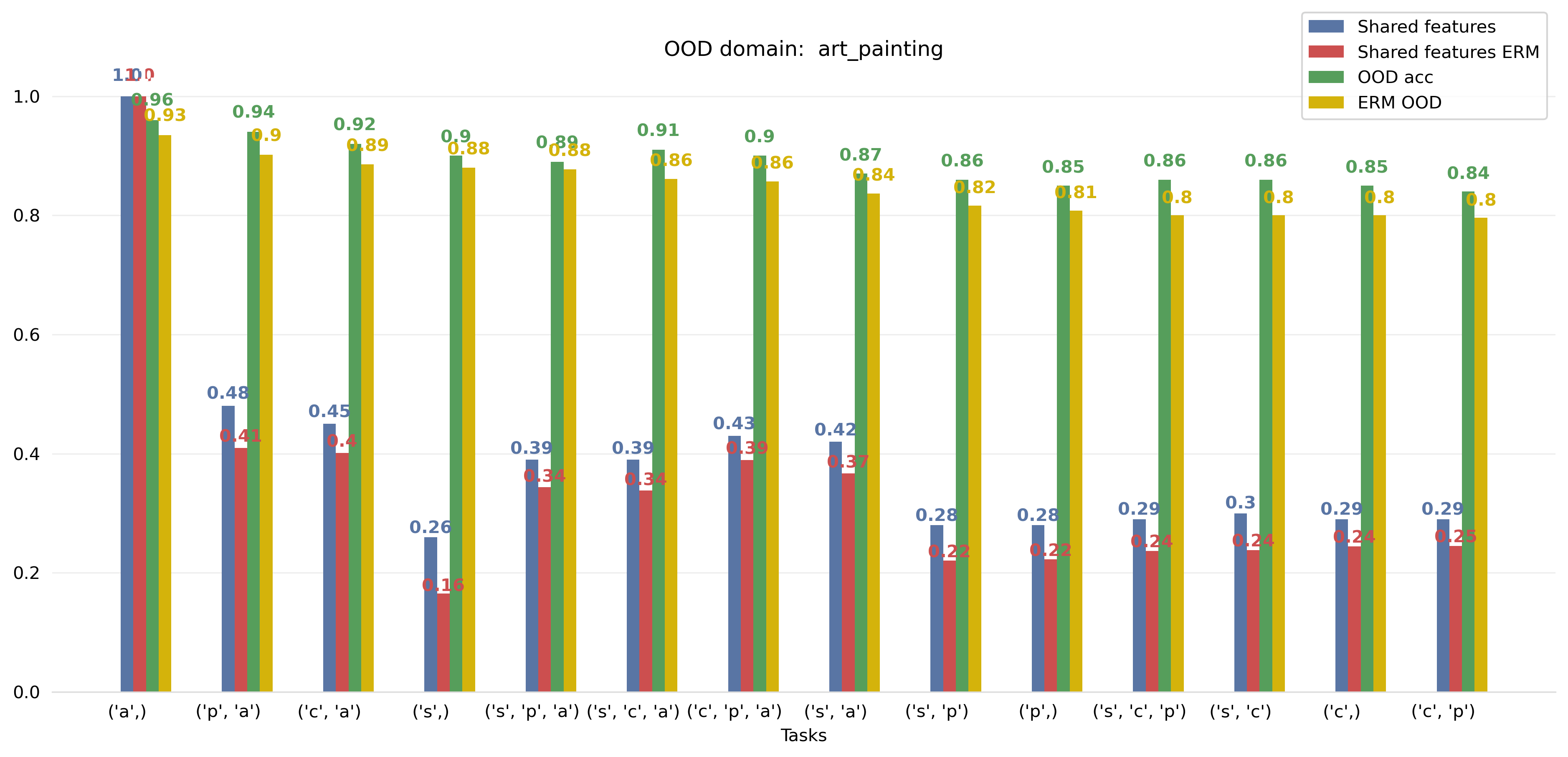
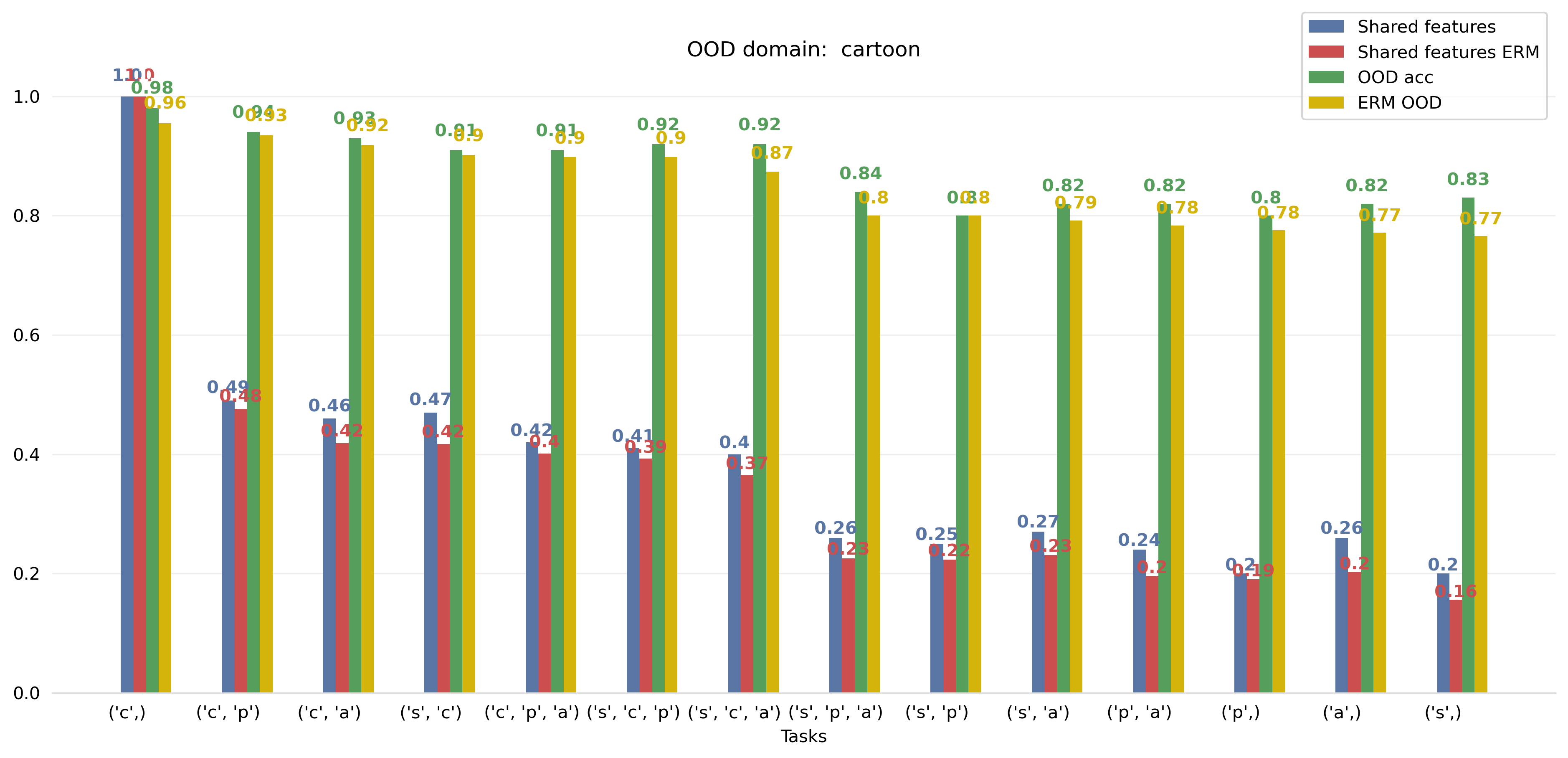
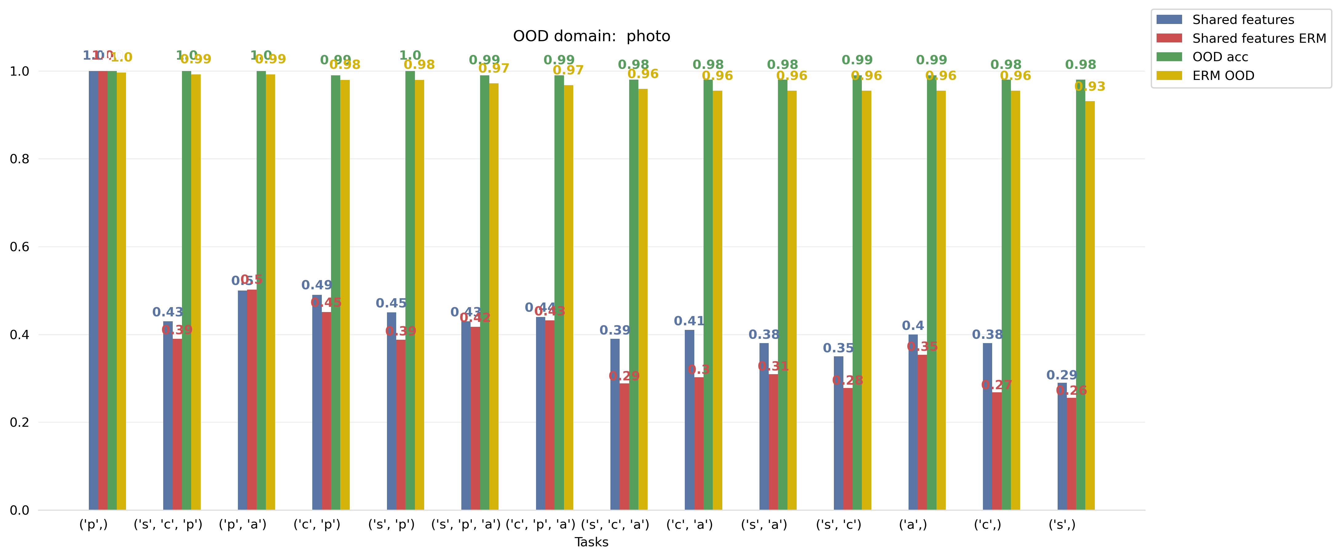
Figure 11: Additional results for all domains in PACS, separated by domain. The overall message of Figure 9 appear consistent across all domains.

D.7 Task similarity

We show that our method enables direct extraction of a task representation and a metric for task similarity from our model and its feature space. We propose to use the coefficients of the fitted linear heads $f_{\phi_{t}^{*}}$ on a given task as a representation for that task. Specifically we transform the optimal coefficients $\phi^{*}$ in a $M$-dimensional vector space (here $M$ is the number of features) by simply computing $\sum_{c}|\phi_{t,m,c}^{*}|$, and discretize them by a threshold $\epsilon$. The resulting binary vectors, together with a distance metric (we choose the Hamming distance), form a discrete metric space of tasks. We preliminary verify how the proposed representation and metric behave on MiniImagenet [88] below.

We sample 160 tasks from 10 groups from , where each group has the same class support, i.e. $t_{1},t_{2}\in G_{i}\mapsto Supp(t_{1})==Supp(t_{2})\forall i.$ We then fit the linear heads independently on each task (i.e. not using the feature sharing regularizer). Then we compute the discrete task representation and project the resulting vector space in a two dimensional vector space using tSNE [92]. The clusters obtained in this space correspond exactly to the group identities (visualized in color in Figure 12).

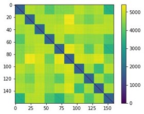
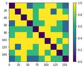
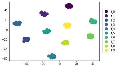
Figure 12: Task Similarity. We visualize the tSNE of the discrete task representation and observe that the clusters in this space corresponds to group identities.

D.8 Comparison with metalearning baselines

In Table 16, we further compare our method on meta learning benchmarks, namely Mini Imagenet [88] and CIFAR-FS [9] with different approaches in the literature based on meta learning [81, 66, 18, 47].

In Figure 13 we compare the predicting performance of our method and capacity to leverage shared knowledge between task, comparing with backbone trained with protopical network approach. We sample a set of task with different overlap, where the overlap between two task $t_{1},t_{2}$ is defined as $sim(t_{1},t_{2})=\frac{Supp(t_{1})\cap Supp(t_{2})}{Supp(t_{1})\cup Supp(t_{2}}$ indicating with $Supp(t_{i})$ the support over classes in task $t_{i}$. We show that other than reaching a much higher accuracy the features of our model are able to be clustered at test time enabling to reach better performance on unseen task. As a matter of fact we can use the feature sharing regularizer at test time showing that there is a increasing trend in the performance, while the prototypical networks features just decreases being unable to share information across tasks at test time.

Table 16: Meta learning baselines, including concurrent work [47] which we significantly outperform.

	Architecture	Cifar-FS (1 shot)	Cifar-FS( 5 shot)	MiniImagenet(1 shot)	MiniImagenet (5 shot)
MAML	Conv32(x4)	-	-	48.7±1.84	63.11±0.66
Prototypical Net	Conv64(x4)	-	-	49.42±0.78	68.20±0.66
TADAM	ResNet12	-	-	58.5 ±0.56	76.7 ±0.3
MetaOptNet	ResNet12	72.0 ± 0.7	84.2 ± 0.5	$\mathbf{62.64}$±0.61	$\mathbf{78.63}$±0.46
MetaBaseline	WRN 28-10	$\mathbf{76.58}$±0.68	85.79±0.5	59.62 ±0.66	78.17 ±0.49
Lachapelle et al[47]	ResNet12	-	-	54.22 ± 0.6	70.01 ± 0.51
Ours*	ResNet12	75.1 ±0.4	$\mathbf{86.9}$ ±0.19	60.1 ± 2	76.6 ± 0.1

D.9 Sharing features at test time

Features can be enforced to be shared also at test time, simply by setting $\beta>0$ to fit the linear head on top of the learned feature space. We observe the benefits of utilizing the feature sharing penalty at test time on the Camelyon17 dataset in the fourth row of Table 17.

As highlighted in the main paper, retaining features which are shared across the training domains and cutting the ones that are domain-specific enable to perform better at test time, at the expenses of lower performance near the training distribution.

We analyzed in more depth this phenomenon in Figure 13. For this experiment we trained our model and a Prototypical network [81] one on the MiniImagenet dataset. Then we sampled 5 groups of tasks according to an average overlap measure between tasks. Between two task $t_{1},t_{2}$ the overlap is defined as $sim(t_{1},t_{2})=\frac{Supp(t_{1})\cap Supp(t_{2})}{Supp(t_{1})\cup Supp(t_{2}}$. each group is made of $10$ task. We then plot the performance at test time increasing the regularization parameter $\beta$, weighting the feature sharing. The outcome of the experiment is twofold: (i) we observe an increase in performance at test time, especially when tasks shows maximal overlap (i.e. they share more features) (ii) this is not the case with the pretrained backbone of [81] which shows almost monotonical decrease in the performance, i.e. enforcing the minimality property during training enables to use it as well at test time.

Further analysis on different datasets, and also on tuning strategies on the regularization parameter are promising directions for future work, to better understand when and how enforcing feature sharing is beneficial at test time.

Table 17: Camelyon17 quantitative results: we report accuracy both on ID and OOD splits. We show (last row) that feature sharing at test time, leads to more robust features on OOD test data.

	Validation(ID)	Validation (OOD)	Test (OOD)
ERM	93.2	84	70.3
CORAL	95.4	86.2	59.5
IRM	91.6	86.2	64.2
Ours	$\mathbf{93.2}$±0.3	$\mathbf{89.9}$±0.6	74.1±0.2
Ours($\beta>0$ test)	${90.4}$±0.2	84.01±0.9	$\mathbf{85.5}$±0.6

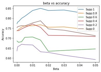
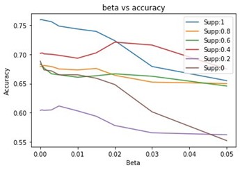
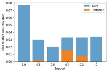
Figure 13: Enforcing feature sharing at test time. Our approach (on the left) is able to benefit from the feature sharing constraint at test time, while using the prototypical network backbone performance monotonically decrease (center). On the right we show the maximal performance gain for each group of tasks for the two approaches.

References

- [1] Julius Adebayo, Justin Gilmer, Michael Muelly, Ian J. Goodfellow, Moritz Hardt, and Been Kim. Sanity checks for saliency maps. In Samy Bengio, Hanna M. Wallach, Hugo Larochelle, Kristen Grauman, Nicolò Cesa-Bianchi, and Roman Garnett, editors, Advances in Neural Information Processing Systems 31: Annual Conference on Neural Information Processing Systems 2018, NeurIPS 2018, December 3-8, 2018, Montréal, Canada, pages 9525–9536, 2018.
- [2] Kartik Ahuja, Karthikeyan Shanmugam, Kush R. Varshney, and Amit Dhurandhar. Invariant risk minimization games. In Proceedings of the 37th International Conference on Machine Learning, ICML 2020, 13-18 July 2020, Virtual Event, volume 119 of Proceedings of Machine Learning Research, pages 145–155, 2020.
- [3] Isabela Albuquerque, João Monteiro, Mohammad Darvishi, Tiago H Falk, and Ioannis Mitliagkas. Generalizing to unseen domains via distribution matching. ArXiv preprint, abs/1911.00804, 2019.
- [4] Martin Arjovsky, Léon Bottou, Ishaan Gulrajani, and David Lopez-Paz. Invariant risk minimization. ArXiv preprint, abs/1907.02893, 2019.
- [5] Jinze Bai, Rui Men, Hao Yang, Xuancheng Ren, Kai Dang, Yichang Zhang, Xiaohuan Zhou, Peng Wang, Sinan Tan, An Yang, et al. Ofasys: A multi-modal multi-task learning system for building generalist models. ArXiv preprint, abs/2212.04408, 2022.
- [6] Peter Bandi. Camelyon17 dataset. GigaScience, 2017.
- [7] Sara Beery, Grant Van Horn, and Pietro Perona. Recognition in terra incognita. In Proceedings of the European conference on computer vision (ECCV), pages 456–473, 2018.
- [8] Yoshua Bengio, Aaron Courville, and Pascal Vincent. Representation learning: A review and new perspectives. IEEE transactions on pattern analysis and machine intelligence, 35(8):1798–1828, 2013.
- [9] Luca Bertinetto, João F. Henriques, Philip H. S. Torr, and Andrea Vedaldi. Meta-learning with differentiable closed-form solvers. In 7th International Conference on Learning Representations, ICLR 2019, New Orleans, LA, USA, May 6-9, 2019, 2019.
- [10] Gilles Blanchard, Aniket Anand Deshmukh, Ürün Dogan, Gyemin Lee, and Clayton Scott. Domain generalization by marginal transfer learning. J. Mach. Learn. Res., 22:2:1–2:55, 2021.
- [11] Mathieu Blondel, Quentin Berthet, Marco Cuturi, Roy Frostig, Stephan Hoyer, Felipe Llinares-López, Fabian Pedregosa, and Jean-Philippe Vert. Efficient and modular implicit differentiation. ArXiv preprint, abs/2105.15183, 2021.
- [12] Daniel Borkan, Lucas Dixon, Jeffrey Sorensen, Nithum Thain, and Lucy Vasserman. Nuanced metrics for measuring unintended bias with real data for text classification. ArXiv preprint, abs/1903.04561, 2019.
- [13] Johann Brehmer, Pim De Haan, Phillip Lippe, and Taco Cohen. Weakly supervised causal representation learning. ArXiv preprint, abs/2203.16437, 2022.
- [14] Chris Burgess and Hyunjik Kim. 3d shapes dataset. https://github.com/deepmind/3dshapes-dataset/, 2018.
- [15] Rich Caruana. Multitask learning. Machine learning, 28(1):41–75, 1997.
- [16] Xi Chen, Yan Duan, Rein Houthooft, John Schulman, Ilya Sutskever, and Pieter Abbeel. Infogan: Interpretable representation learning by information maximizing generative adversarial nets. In Daniel D. Lee, Masashi Sugiyama, Ulrike von Luxburg, Isabelle Guyon, and Roman Garnett, editors, Advances in Neural Information Processing Systems 29: Annual Conference on Neural Information Processing Systems 2016, December 5-10, 2016, Barcelona, Spain, pages 2172–2180, 2016.
- [17] Jia Deng, Wei Dong, Richard Socher, Li-Jia Li, Kai Li, and Fei-Fei Li. Imagenet: A large-scale hierarchical image database. In 2009 IEEE Computer Society Conference on Computer Vision and Pattern Recognition (CVPR 2009), 20-25 June 2009, Miami, Florida, USA, pages 248–255, 2009.
- [18] Guneet Singh Dhillon, Pratik Chaudhari, Avinash Ravichandran, and Stefano Soatto. A baseline for few-shot image classification. In 8th International Conference on Learning Representations, ICLR 2020, Addis Ababa, Ethiopia, April 26-30, 2020, 2020.
- [19] Andrea Dittadi, Frederik Träuble, Francesco Locatello, Manuel Wuthrich, Vaibhav Agrawal, Ole Winther, Stefan Bauer, and Bernhard Schölkopf. On the transfer of disentangled representations in realistic settings. In 9th International Conference on Learning Representations, ICLR 2021, Virtual Event, Austria, May 3-7, 2021, 2021.
- [20] Lucas Dixon, John Li, Jeffrey Sorensen, Nithum Thain, and Lucy Vasserman. Measuring and mitigating unintended bias in text classification. 2018.
- [21] Alexey Dosovitskiy and Josip Djolonga. You only train once: Loss-conditional training of deep networks. In 8th International Conference on Learning Representations, ICLR 2020, Addis Ababa, Ethiopia, April 26-30, 2020, 2020.
- [22] Cian Eastwood and Christopher K. I. Williams. A framework for the quantitative evaluation of disentangled representations. In 6th International Conference on Learning Representations, ICLR 2018, Vancouver, BC, Canada, April 30 - May 3, 2018, Conference Track Proceedings, 2018.
- [23] M. Everingham, L. Van Gool, C. K. I. Williams, J. Winn, and A. Zisserman. The PASCAL Visual Object Classes Challenge 2007 (VOC2007) Results. http://www.pascal-network.org/challenges/VOC/voc2007/workshop/index.html.
- [24] Li Fei-Fei, Rob Fergus, and Pietro Perona. Learning generative visual models from few training examples: An incremental bayesian approach tested on 101 object categories. In 2004 conference on computer vision and pattern recognition workshop, pages 178–178. IEEE, 2004.
- [25] Marco Fumero, Luca Cosmo, Simone Melzi, and Emanuele Rodolà. Learning disentangled representations via product manifold projection. In Marina Meila and Tong Zhang, editors, Proceedings of the 38th International Conference on Machine Learning, ICML 2021, 18-24 July 2021, Virtual Event, volume 139 of Proceedings of Machine Learning Research, pages 3530–3540, 2021.
- [26] Yaroslav Ganin, Evgeniya Ustinova, Hana Ajakan, Pascal Germain, Hugo Larochelle, François Laviolette, Mario Marchand, and Victor Lempitsky. Domain-adversarial training of neural networks. The journal of machine learning research, 17(1):2096–2030, 2016.
- [27] Robert Geirhos, Jörn-Henrik Jacobsen, Claudio Michaelis, Richard Zemel, Wieland Brendel, Matthias Bethge, and Felix A Wichmann. Shortcut learning in deep neural networks. Nature Machine Intelligence, 2(11):665–673, 2020.
- [28] Zhengyang Geng, Xin-Yu Zhang, Shaojie Bai, Yisen Wang, and Zhouchen Lin. On training implicit models. In Marc’Aurelio Ranzato, Alina Beygelzimer, Yann N. Dauphin, Percy Liang, and Jennifer Wortman Vaughan, editors, Advances in Neural Information Processing Systems 34: Annual Conference on Neural Information Processing Systems 2021, NeurIPS 2021, December 6-14, 2021, virtual, pages 24247–24260, 2021.
- [29] Ian J. Goodfellow, Quoc V. Le, Andrew M. Saxe, Honglak Lee, and Andrew Y. Ng. Measuring invariances in deep networks. In Yoshua Bengio, Dale Schuurmans, John D. Lafferty, Christopher K. I. Williams, and Aron Culotta, editors, Advances in Neural Information Processing Systems 22: 23rd Annual Conference on Neural Information Processing Systems 2009. Proceedings of a meeting held 7-10 December 2009, Vancouver, British Columbia, Canada, pages 646–654, 2009.
- [30] Anirudh Goyal, Alex Lamb, Jordan Hoffmann, Shagun Sodhani, Sergey Levine, Yoshua Bengio, and Bernhard Schölkopf. Recurrent independent mechanisms. In 9th International Conference on Learning Representations, ICLR 2021, Virtual Event, Austria, May 3-7, 2021, 2021.
- [31] Andreas Griewank and Andrea Walther. Evaluating derivatives: principles and techniques of algorithmic differentiation. 2008.
- [32] Ishaan Gulrajani and David Lopez-Paz. In search of lost domain generalization. In 9th International Conference on Learning Representations, ICLR 2021, Virtual Event, Austria, May 3-7, 2021, 2021.
- [33] Irina Higgins, Loïc Matthey, Arka Pal, Christopher Burgess, Xavier Glorot, Matthew Botvinick, Shakir Mohamed, and Alexander Lerchner. beta-vae: Learning basic visual concepts with a constrained variational framework. In 5th International Conference on Learning Representations, ICLR 2017, Toulon, France, April 24-26, 2017, Conference Track Proceedings, 2017.
- [34] Timothy Hospedales, Antreas Antoniou, Paul Micaelli, and Amos Storkey. Meta-learning in neural networks: A survey. ArXiv preprint, abs/2004.05439, 2020.
- [35] Ziniu Hu, Zhe Zhao, Xinyang Yi, Tiansheng Yao, Lichan Hong, Yizhou Sun, and Ed H Chi. Improving multi-task generalization via regularizing spurious correlation. ArXiv preprint, abs/2205.09797, 2022.
- [36] Zeyi Huang, Haohan Wang, Eric P Xing, and Dong Huang. Self-challenging improves cross-domain generalization. In Computer Vision–ECCV 2020: 16th European Conference, Glasgow, UK, August 23–28, 2020, Proceedings, Part II 16, pages 124–140. Springer, 2020.
- [37] Aapo Hyvärinen, Hiroaki Sasaki, and Richard E. Turner. Nonlinear ICA using auxiliary variables and generalized contrastive learning. In Kamalika Chaudhuri and Masashi Sugiyama, editors, The 22nd International Conference on Artificial Intelligence and Statistics, AISTATS 2019, 16-18 April 2019, Naha, Okinawa, Japan, volume 89 of Proceedings of Machine Learning Research, pages 859–868, 2019.
- [38] Ali Jalali, Pradeep Ravikumar, Sujay Sanghavi, and Chao Ruan. A dirty model for multi-task learning. In John D. Lafferty, Christopher K. I. Williams, John Shawe-Taylor, Richard S. Zemel, and Aron Culotta, editors, Advances in Neural Information Processing Systems 23: 24th Annual Conference on Neural Information Processing Systems 2010. Proceedings of a meeting held 6-9 December 2010, Vancouver, British Columbia, Canada, pages 964–972, 2010.
- [39] Hicham Janati, Marco Cuturi, and Alexandre Gramfort. Wasserstein regularization for sparse multi-task regression. In Kamalika Chaudhuri and Masashi Sugiyama, editors, The 22nd International Conference on Artificial Intelligence and Statistics, AISTATS 2019, 16-18 April 2019, Naha, Okinawa, Japan, volume 89 of Proceedings of Machine Learning Research, pages 1407–1416, 2019.
- [40] Yibo Jiang and Victor Veitch. Invariant and transportable representations for anti-causal domain shifts, 2022.
- [41] Ilyes Khemakhem, Diederik P. Kingma, Ricardo Pio Monti, and Aapo Hyvärinen. Variational autoencoders and nonlinear ICA: A unifying framework. In Silvia Chiappa and Roberto Calandra, editors, The 23rd International Conference on Artificial Intelligence and Statistics, AISTATS 2020, 26-28 August 2020, Online [Palermo, Sicily, Italy], volume 108 of Proceedings of Machine Learning Research, pages 2207–2217, 2020.
- [42] Diederik P. Kingma and Jimmy Ba. Adam: A method for stochastic optimization. In Yoshua Bengio and Yann LeCun, editors, 3rd International Conference on Learning Representations, ICLR 2015, San Diego, CA, USA, May 7-9, 2015, Conference Track Proceedings, 2015.
- [43] Polina Kirichenko, Pavel Izmailov, and Andrew Gordon Wilson. Last layer re-training is sufficient for robustness to spurious correlations. ArXiv preprint, abs/2204.02937, 2022.
- [44] Pang Wei Koh, Shiori Sagawa, Henrik Marklund, Sang Michael Xie, Marvin Zhang, Akshay Balsubramani, Weihua Hu, Michihiro Yasunaga, Richard Lanas Phillips, Irena Gao, Tony Lee, Etienne David, Ian Stavness, Wei Guo, Berton Earnshaw, Imran S. Haque, Sara M. Beery, Jure Leskovec, Anshul Kundaje, Emma Pierson, Sergey Levine, Chelsea Finn, and Percy Liang. WILDS: A benchmark of in-the-wild distribution shifts. In Marina Meila and Tong Zhang, editors, Proceedings of the 38th International Conference on Machine Learning, ICML 2021, 18-24 July 2021, Virtual Event, volume 139 of Proceedings of Machine Learning Research, pages 5637–5664, 2021.
- [45] David Krueger, Ethan Caballero, Jörn-Henrik Jacobsen, Amy Zhang, Jonathan Binas, Dinghuai Zhang, Rémi Le Priol, and Aaron C. Courville. Out-of-distribution generalization via risk extrapolation (rex). In Marina Meila and Tong Zhang, editors, Proceedings of the 38th International Conference on Machine Learning, ICML 2021, 18-24 July 2021, Virtual Event, volume 139 of Proceedings of Machine Learning Research, pages 5815–5826, 2021.
- [46] Tejas D. Kulkarni, William F. Whitney, Pushmeet Kohli, and Joshua B. Tenenbaum. Deep convolutional inverse graphics network. In Corinna Cortes, Neil D. Lawrence, Daniel D. Lee, Masashi Sugiyama, and Roman Garnett, editors, Advances in Neural Information Processing Systems 28: Annual Conference on Neural Information Processing Systems 2015, December 7-12, 2015, Montreal, Quebec, Canada, pages 2539–2547, 2015.
- [47] Sébastien Lachapelle, Tristan Deleu, Divyat Mahajan, Ioannis Mitliagkas, Yoshua Bengio, Simon Lacoste-Julien, and Quentin Bertrand. Synergies between disentanglement and sparsity: a multi-task learning perspective. ArXiv preprint, abs/2211.14666, 2022.
- [48] Sébastien Lachapelle, Pau Rodriguez, Yash Sharma, Katie E Everett, Rémi Le Priol, Alexandre Lacoste, and Simon Lacoste-Julien. Disentanglement via mechanism sparsity regularization: A new principle for nonlinear ica. In Conference on Causal Learning and Reasoning, pages 428–484. PMLR, 2022.
- [49] Yann LeCun, Fu Jie Huang, and Leon Bottou. Learning methods for generic object recognition with invariance to pose and lighting. In Proceedings of the 2004 IEEE Computer Society Conference on Computer Vision and Pattern Recognition, 2004. CVPR 2004., volume 2, pages II–104. IEEE, 2004.
- [50] Kwonjoon Lee, Subhransu Maji, Avinash Ravichandran, and Stefano Soatto. Meta-learning with differentiable convex optimization. In IEEE Conference on Computer Vision and Pattern Recognition, CVPR 2019, Long Beach, CA, USA, June 16-20, 2019, pages 10657–10665, 2019.
- [51] Da Li, Yongxin Yang, Yi-Zhe Song, and Timothy M. Hospedales. Deeper, broader and artier domain generalization. In IEEE International Conference on Computer Vision, ICCV 2017, Venice, Italy, October 22-29, 2017, pages 5543–5551, 2017.
- [52] Da Li, Yongxin Yang, Yi-Zhe Song, and Timothy M. Hospedales. Learning to generalize: Meta-learning for domain generalization. In Sheila A. McIlraith and Kilian Q. Weinberger, editors, Proceedings of the Thirty-Second AAAI Conference on Artificial Intelligence, (AAAI-18), the 30th innovative Applications of Artificial Intelligence (IAAI-18), and the 8th AAAI Symposium on Educational Advances in Artificial Intelligence (EAAI-18), New Orleans, Louisiana, USA, February 2-7, 2018, pages 3490–3497, 2018.
- [53] Haoliang Li, Sinno Jialin Pan, Shiqi Wang, and Alex C. Kot. Domain generalization with adversarial feature learning. In 2018 IEEE Conference on Computer Vision and Pattern Recognition, CVPR 2018, Salt Lake City, UT, USA, June 18-22, 2018, pages 5400–5409, 2018.
- [54] Ya Li, Xinmei Tian, Mingming Gong, Yajing Liu, Tongliang Liu, Kun Zhang, and Dacheng Tao. Deep domain generalization via conditional invariant adversarial networks. In Proceedings of the European conference on computer vision (ECCV), pages 624–639, 2018.
- [55] Phillip Lippe, Sara Magliacane, Sindy Löwe, Yuki M. Asano, Taco Cohen, and Stratis Gavves. CITRIS: causal identifiability from temporal intervened sequences. In Kamalika Chaudhuri, Stefanie Jegelka, Le Song, Csaba Szepesvári, Gang Niu, and Sivan Sabato, editors, International Conference on Machine Learning, ICML 2022, 17-23 July 2022, Baltimore, Maryland, USA, volume 162 of Proceedings of Machine Learning Research, pages 13557–13603, 2022.
- [56] Francesco Locatello, Stefan Bauer, Mario Lucic, Gunnar Rätsch, Sylvain Gelly, Bernhard Schölkopf, and Olivier Bachem. Challenging common assumptions in the unsupervised learning of disentangled representations. In Kamalika Chaudhuri and Ruslan Salakhutdinov, editors, Proceedings of the 36th International Conference on Machine Learning, ICML 2019, 9-15 June 2019, Long Beach, California, USA, volume 97 of Proceedings of Machine Learning Research, pages 4114–4124, 2019.
- [57] Francesco Locatello, Stefan Bauer, Mario Lucic, Gunnar Rätsch, Sylvain Gelly, Bernhard Schölkopf, and Olivier Bachem. A sober look at the unsupervised learning of disentangled representations and their evaluation. J. Mach. Learn. Res., 21:209:1–209:62, 2020.
- [58] Francesco Locatello, Ben Poole, Gunnar Rätsch, Bernhard Schölkopf, Olivier Bachem, and Michael Tschannen. Weakly-supervised disentanglement without compromises. In Proceedings of the 37th International Conference on Machine Learning, ICML 2020, 13-18 July 2020, Virtual Event, volume 119 of Proceedings of Machine Learning Research, pages 6348–6359, 2020.
- [59] Aurelie C. Lozano and Grzegorz Swirszcz. Multi-level lasso for sparse multi-task regression. In Proceedings of the 29th International Conference on Machine Learning, ICML 2012, Edinburgh, Scotland, UK, June 26 - July 1, 2012, 2012.
- [60] Chaochao Lu, Yuhuai Wu, José Miguel Hernández-Lobato, and Bernhard Schölkopf. Invariant causal representation learning for out-of-distribution generalization. In The Tenth International Conference on Learning Representations, ICLR 2022, Virtual Event, April 25-29, 2022, 2022.
- [61] Zvika Marx, Michael T Rosenstein, Leslie Pack Kaelbling, and Thomas G Dietterich. Transfer learning with an ensemble of background tasks. Inductive Transfer, 10, 2005.
- [62] Loic Matthey, Irina Higgins, Demis Hassabis, and Alexander Lerchner. dsprites: Disentanglement testing sprites dataset. https://github.com/deepmind/dsprites-dataset/, 2017.
- [63] John Miller, Rohan Taori, Aditi Raghunathan, Shiori Sagawa, Pang Wei Koh, Vaishaal Shankar, Percy Liang, Yair Carmon, and Ludwig Schmidt. Accuracy on the line: on the strong correlation between out-of-distribution and in-distribution generalization. In Marina Meila and Tong Zhang, editors, Proceedings of the 38th International Conference on Machine Learning, ICML 2021, 18-24 July 2021, Virtual Event, volume 139 of Proceedings of Machine Learning Research, pages 7721–7735, 2021.
- [64] Krikamol Muandet, David Balduzzi, and Bernhard Schölkopf. Domain generalization via invariant feature representation. In Proceedings of the 30th International Conference on Machine Learning, ICML 2013, Atlanta, GA, USA, 16-21 June 2013, volume 28 of JMLR Workshop and Conference Proceedings, pages 10–18, 2013.
- [65] Hyeonseob Nam, HyunJae Lee, Jongchan Park, Wonjun Yoon, and Donggeun Yoo. Reducing domain gap by reducing style bias. In IEEE Conference on Computer Vision and Pattern Recognition, CVPR 2021, virtual, June 19-25, 2021, pages 8690–8699, 2021.
- [66] Boris N. Oreshkin, Pau Rodríguez López, and Alexandre Lacoste. TADAM: task dependent adaptive metric for improved few-shot learning. In Samy Bengio, Hanna M. Wallach, Hugo Larochelle, Kristen Grauman, Nicolò Cesa-Bianchi, and Roman Garnett, editors, Advances in Neural Information Processing Systems 31: Annual Conference on Neural Information Processing Systems 2018, NeurIPS 2018, December 3-8, 2018, Montréal, Canada, pages 719–729, 2018.
- [67] Giambattista Parascandolo, Niki Kilbertus, Mateo Rojas-Carulla, and Bernhard Schölkopf. Learning independent causal mechanisms. In Jennifer G. Dy and Andreas Krause, editors, Proceedings of the 35th International Conference on Machine Learning, ICML 2018, Stockholmsmässan, Stockholm, Sweden, July 10-15, 2018, volume 80 of Proceedings of Machine Learning Research, pages 4033–4041, 2018.
- [68] Ji Ho Park, Jamin Shin, and Pascale Fung. Reducing gender bias in abusive language detection. In Proceedings of the 2018 Conference on Empirical Methods in Natural Language Processing, pages 2799–2804, 2018.
- [69] Adam Paszke, Sam Gross, Francisco Massa, Adam Lerer, James Bradbury, Gregory Chanan, Trevor Killeen, Zeming Lin, Natalia Gimelshein, Luca Antiga, Alban Desmaison, Andreas Köpf, Edward Yang, Zachary DeVito, Martin Raison, Alykhan Tejani, Sasank Chilamkurthy, Benoit Steiner, Lu Fang, Junjie Bai, and Soumith Chintala. Pytorch: An imperative style, high-performance deep learning library. In Hanna M. Wallach, Hugo Larochelle, Alina Beygelzimer, Florence d’Alché-Buc, Emily B. Fox, and Roman Garnett, editors, Advances in Neural Information Processing Systems 32: Annual Conference on Neural Information Processing Systems 2019, NeurIPS 2019, December 8-14, 2019, Vancouver, BC, Canada, pages 8024–8035, 2019.
- [70] Jielin Qiu, Yi Zhu, Xingjian Shi, Florian Wenzel, Zhiqiang Tang, Ding Zhao, Bo Li, and Mu Li. Are multimodal models robust to image and text perturbations? ArXiv preprint, abs/2212.08044, 2022.
- [71] Scott E. Reed, Yi Zhang, Yuting Zhang, and Honglak Lee. Deep visual analogy-making. In Corinna Cortes, Neil D. Lawrence, Daniel D. Lee, Masashi Sugiyama, and Roman Garnett, editors, Advances in Neural Information Processing Systems 28: Annual Conference on Neural Information Processing Systems 2015, December 7-12, 2015, Montreal, Quebec, Canada, pages 1252–1260, 2015.
- [72] Bryan C Russell, Antonio Torralba, Kevin P Murphy, and William T Freeman. Labelme: a database and web-based tool for image annotation. International journal of computer vision, 77(1):157–173, 2008.
- [73] Shiori Sagawa, Pang Wei Koh, Tatsunori B. Hashimoto, and Percy Liang. Distributionally robust neural networks for group shifts: On the importance of regularization for worst-case generalization. ArXiv preprint, abs/1911.08731, 2019.
- [74] Shiori Sagawa, Aditi Raghunathan, Pang Wei Koh, and Percy Liang. An investigation of why overparameterization exacerbates spurious correlations. In Proceedings of the 37th International Conference on Machine Learning, ICML 2020, 13-18 July 2020, Virtual Event, volume 119 of Proceedings of Machine Learning Research, pages 8346–8356, 2020.
- [75] Ruslan Salakhutdinov. Deep learning. In Sofus A. Macskassy, Claudia Perlich, Jure Leskovec, Wei Wang, and Rayid Ghani, editors, The 20th ACM SIGKDD International Conference on Knowledge Discovery and Data Mining, KDD ’14, New York, NY, USA - August 24 - 27, 2014, page 1973, 2014.
- [76] Victor Sanh, Lysandre Debut, Julien Chaumond, and Thomas Wolf. Distilbert, a distilled version of bert: smaller, faster, cheaper and lighter. ArXiv preprint, abs/1910.01108, 2019.
- [77] Jürgen Schmidhuber. Learning factorial codes by predictability minimization. Neural computation, 4(6):863–879, 1992.
- [78] Bernhard Schölkopf, Francesco Locatello, Stefan Bauer, Nan Rosemary Ke, Nal Kalchbrenner, Anirudh Goyal, and Yoshua Bengio. Toward causal representation learning. Proceedings of the IEEE, 109(5):612–634, 2021.
- [79] Anna Seigal, Chandler Squires, and Caroline Uhler. Linear causal disentanglement via interventions. ArXiv preprint, abs/2211.16467, 2022.
- [80] Amanpreet Singh, Ronghang Hu, Vedanuj Goswami, Guillaume Couairon, Wojciech Galuba, Marcus Rohrbach, and Douwe Kiela. FLAVA: A foundational language and vision alignment model. ArXiv preprint, abs/2112.04482, 2021.
- [81] Jake Snell, Kevin Swersky, and Richard S. Zemel. Prototypical networks for few-shot learning. In Isabelle Guyon, Ulrike von Luxburg, Samy Bengio, Hanna M. Wallach, Rob Fergus, S. V. N. Vishwanathan, and Roman Garnett, editors, Advances in Neural Information Processing Systems 30: Annual Conference on Neural Information Processing Systems 2017, December 4-9, 2017, Long Beach, CA, USA, pages 4077–4087, 2017.
- [82] Peter Sorrenson, Carsten Rother, and Ullrich Köthe. Disentanglement by nonlinear ICA with general incompressible-flow networks (GIN). In 8th International Conference on Learning Representations, ICLR 2020, Addis Ababa, Ethiopia, April 26-30, 2020, 2020.
- [83] Trevor Standley, Amir Roshan Zamir, Dawn Chen, Leonidas J. Guibas, Jitendra Malik, and Silvio Savarese. Which tasks should be learned together in multi-task learning? In Proceedings of the 37th International Conference on Machine Learning, ICML 2020, 13-18 July 2020, Virtual Event, volume 119 of Proceedings of Machine Learning Research, pages 9120–9132, 2020.
- [84] Baochen Sun, Jiashi Feng, and Kate Saenko. Correlation alignment for unsupervised domain adaptation. In Domain Adaptation in Computer Vision Applications, pages 153–171. 2017.
- [85] Baochen Sun and Kate Saenko. Deep coral: Correlation alignment for deep domain adaptation. In European conference on computer vision, pages 443–450. Springer, 2016.
- [86] Victor Veitch, Alexander D’Amour, Steve Yadlowsky, and Jacob Eisenstein. Counterfactual invariance to spurious correlations: Why and how to pass stress tests, 2021.
- [87] Hemanth Venkateswara, Jose Eusebio, Shayok Chakraborty, and Sethuraman Panchanathan. Deep hashing network for unsupervised domain adaptation. In 2017 IEEE Conference on Computer Vision and Pattern Recognition, CVPR 2017, Honolulu, HI, USA, July 21-26, 2017, pages 5385–5394, 2017.
- [88] Oriol Vinyals, Charles Blundell, Tim Lillicrap, Koray Kavukcuoglu, and Daan Wierstra. Matching networks for one shot learning. In Daniel D. Lee, Masashi Sugiyama, Ulrike von Luxburg, Isabelle Guyon, and Roman Garnett, editors, Advances in Neural Information Processing Systems 29: Annual Conference on Neural Information Processing Systems 2016, December 5-10, 2016, Barcelona, Spain, pages 3630–3638, 2016.
- [89] C. Wah, S. Branson, P. Welinder, P. Perona, and S. Belongie. The caltech-ucsd birds-200-2011 dataset. Technical Report CNS-TR-2011-001, California Institute of Technology, 2011.
- [90] Zihao Wang and Victor Veitch. A unified causal view of domain invariant representation learning. ArXiv preprint, abs/2208.06987, 2022.
- [91] Zirui Wang, Zihang Dai, Barnabás Póczos, and Jaime G. Carbonell. Characterizing and avoiding negative transfer. In IEEE Conference on Computer Vision and Pattern Recognition, CVPR 2019, Long Beach, CA, USA, June 16-20, 2019, pages 11293–11302, 2019.
- [92] Martin Wattenberg, Fernanda Viégas, and Ian Johnson. How to use t-sne effectively. Distill, 1(10):e2, 2016.
- [93] Florian Wenzel, Andrea Dittadi, Peter V. Gehler, Carl-Johann Simon-Gabriel, Max Horn, Dominik Zietlow, David Kernert, Chris Russell, Thomas Brox, Bernt Schiele, Bernhard Schölkopf, and Francesco Locatello. Assaying out-of-distribution generalization in transfer learning. In Neural Information Processing Systems, 2022.
- [94] Olivia Wiles, Sven Gowal, Florian Stimberg, Sylvestre-Alvise Rebuffi, Ira Ktena, Krishnamurthy Dvijotham, and Ali Taylan Cemgil. A fine-grained analysis on distribution shift. In The Tenth International Conference on Learning Representations, ICLR 2022, Virtual Event, April 25-29, 2022, 2022.
- [95] Matthew Willetts and Brooks Paige. I don’t need u: Identifiable non-linear ica without side information. ArXiv preprint, abs/2106.05238, 2021.
- [96] Thomas Wolf, Lysandre Debut, Victor Sanh, Julien Chaumond, Clement Delangue, Anthony Moi, Pierric Cistac, Tim Rault, Rémi Louf, Morgan Funtowicz, et al. Huggingface’s transformers: State-of-the-art natural language processing. ArXiv preprint, abs/1910.03771, 2019.
- [97] Mitchell Wortsman, Gabriel Ilharco, Samir Yitzhak Gadre, Rebecca Roelofs, Raphael Gontijo Lopes, Ari S. Morcos, Hongseok Namkoong, Ali Farhadi, Yair Carmon, Simon Kornblith, and Ludwig Schmidt. Model soups: averaging weights of multiple fine-tuned models improves accuracy without increasing inference time. In Kamalika Chaudhuri, Stefanie Jegelka, Le Song, Csaba Szepesvári, Gang Niu, and Sivan Sabato, editors, International Conference on Machine Learning, ICML 2022, 17-23 July 2022, Baltimore, Maryland, USA, volume 162 of Proceedings of Machine Learning Research, pages 23965–23998, 2022.
- [98] Jianxiong Xiao, James Hays, Krista A. Ehinger, Aude Oliva, and Antonio Torralba. SUN database: Large-scale scene recognition from abbey to zoo. In The Twenty-Third IEEE Conference on Computer Vision and Pattern Recognition, CVPR 2010, San Francisco, CA, USA, 13-18 June 2010, pages 3485–3492, 2010.
- [99] Shen Yan, Huan Song, Nanxiang Li, Lincan Zou, and Liu Ren. Improve unsupervised domain adaptation with mixup training. ArXiv preprint, abs/2001.00677, 2020.
- [100] Weiran Yao, Yuewen Sun, Alex Ho, Changyin Sun, and Kun Zhang. Learning temporally causal latent processes from general temporal data. In The Tenth International Conference on Learning Representations, ICLR 2022, Virtual Event, April 25-29, 2022, 2022.
- [101] Lu Yuan, Dongdong Chen, Yi-Ling Chen, Noel Codella, Xiyang Dai, Jianfeng Gao, Houdong Hu, Xuedong Huang, Boxin Li, Chunyuan Li, Ce Liu, Mengchen Liu, Zicheng Liu, Yumao Lu, Yu Shi, Lijuan Wang, Jianfeng Wang, Bin Xiao, Zhen Xiao, Jianwei Yang, Michael Zeng, Luowei Zhou, and Pengchuan Zhang. Florence: A new foundation model for computer vision. ArXiv preprint, abs/2111.11432, 2021.
- [102] Marvin Zhang, Henrik Marklund, Nikita Dhawan, Abhishek Gupta, Sergey Levine, and Chelsea Finn. Adaptive risk minimization: Learning to adapt to domain shift. In Marc’Aurelio Ranzato, Alina Beygelzimer, Yann N. Dauphin, Percy Liang, and Jennifer Wortman Vaughan, editors, Advances in Neural Information Processing Systems 34: Annual Conference on Neural Information Processing Systems 2021, NeurIPS 2021, December 6-14, 2021, virtual, pages 23664–23678, 2021.
- [103] Yu Zhang and Qiang Yang. An overview of multi-task learning. National Science Review, 5(1):30–43, 2018.
- [104] Bolei Zhou, Agata Lapedriza, Aditya Khosla, Aude Oliva, and Antonio Torralba. Places: A 10 million image database for scene recognition. IEEE transactions on pattern analysis and machine intelligence, 40(6):1452–1464, 2017.
- [105] Kaiyang Zhou, Ziwei Liu, Yu Qiao, Tao Xiang, and Chen Change Loy. Domain generalization: A survey. IEEE Trans. Pattern Anal. Mach. Intell., 45(4):4396–4415, August 2022.
- [106] Jinguo Zhu, Xizhou Zhu, Wenhai Wang, Xiaohua Wang, Hongsheng Li, Xiaogang Wang, and Jifeng Dai. Uni-perceiver-moe: Learning sparse generalist models with conditional moes. ArXiv preprint, abs/2206.04674, 2022.