Counting geodesics on expander surfaces

Abstract

We study properties of typical closed geodesics on expander surfaces of high genus, i.e. closed hyperbolic surfaces with a uniform spectral gap of the Laplacian. Under an additional systole lower bound assumption, we show almost every geodesic of length much greater than $\sqrt{g}\log g$ is non-simple. And we prove almost every closed geodesic of length much greater than $g(\log g)^{2}$ is filling, i.e. each component of the complement of the geodesic is a topological disc. Our results apply to Weil-Petersson random surfaces, random covers of a fixed surface, and Brooks-Makover random surfaces, since these models are known to have uniform spectral gap asymptotically almost surely.

Our proof technique involves adapting Margulis’ counting strategy to work at low length scales.

1 Introduction

Let $X$ be a connected, closed, orientable hyperbolic surface. It is easy to see that the shortest closed geodesic on $X$ is always simple, i.e. does not self-intersect. The number of simple geodesics less than a given length grows polynomially [Riv01, Mir08], while the total number of closed geodesics grows exponentially (by work of Delsarte, Huber, and Selberg; see [Bus10] for references). Thus non-simple closed geodesics must eventually become predominant. At what length scale does the transition occur?

We refer to this as the “birthday problem” for geodesics, by analogy with the basic probability question about the number of uniform, independent samples with replacement from a collection of $n$ objects needed before some object is picked multiple times. The answer will depend on particular geometric features of the surface. In this paper, we address this question for expander surfaces. We also study the question of the length scale at which almost all closed geodesics are filling, i.e. each component of the complement of the geodesic (projected to the surface $X$) is a topological disc.

The Laplace operator on $X$ has a discrete spectrum and always has a simple eigenvalue of $0$. The spectral gap is the distance to the next smallest eigenvalue. For $\delta>0$ we say that $X$ is a $\delta$-expander surface if its spectral gap is greater than $\delta$. This terminology is motivated by an analogous and much studied concept for graphs. Families of $\delta$-expander surfaces exhibit many interesting properties such as fast mixing of geodesic flow and lower bound on Cheeger constant. Random constructions typically give expander families.

We denote by $N(X,L)$, respectively $N_{simp}(X,L)$, the number of closed geodesics, respectively simple closed geodesics, on $X$ of length at most $L$. The systole of a hyperbolic surface is the length of the shortest closed geodesic.

Theorem 1.1.

Let $\delta,s_{0},\epsilon>0$. There exists a constant $c=c(\delta,s_{0},\epsilon)$ such that for any $\delta$-expander surface $X$ of genus $g$ with systole at least $s_{0}$, and any $L>c\sqrt{g}\log g$,

$$N_{simp}(X,L)\leq\epsilon\cdot N(X,L).$$

Conjecture 1.2.

In the above, one can replace the condition $L>c\sqrt{g}\log g$ by $L>c\sqrt{g}$.

Wu and Xue have recently proved the analogous conjecture for the specific case of Weil-Petersson random surfaces [WX22, Theorem 4, part (2)].

It is also conceivable that the theorem (and conjecture) hold for all surfaces $X$ (with no assumption about spectral gap or systole).

Asymptotic notation.

In this paper, we use Hardy’s notation $A\prec B$ to mean $A=o(B)$ as the independent variable (typically the genus $g$) goes to $\infty$.

Remark 1.3.

For the regime $L\prec\sqrt{g}$, whether $N_{simp}(X,L)$ is dominant depends on more aspects of the geometry of the surface, beyond spectral gap and systole lower bound.

On the one hand, in this regime Weil-Petersson random surfaces will have $N_{simp}(X,L)>(1-\epsilon)N(X,L)$ asymptotically almost surely [WX22, Theorem 4 (1)].

On the other hand, surfaces obtained by gluing fixed hyperbolic pairs of pants (say with all cuffs of length $2$) according to a random regular graph, with any twists, asymptotically almost surely form an expander family with lower bound on systole. This follows by combining (i) a comparison of the Cheeger constant for the surface to that of the graph [Bus78, Section 4.1], and (ii) the well-known lower bound on Cheeger constant for random regular graphs. For these surfaces, we anticipate that $N_{simp}(X,L)\prec N(X,L)$ whenever $L\to\infty$ with $g$ (so including many cases in which $L\prec\sqrt{g}$), since every time a geodesic enters a pair of pants it has a definite chance of picking up a self-intersection before leaving. ∎

Let $N_{fill}(X,L)$ denote the number of filling closed geodesics on $X$ of length at most $L$.

Theorem 1.4.

Let $\delta,s_{0},\epsilon>0$. There exists a constant $c=c(\delta,s_{0},\epsilon)$ such that for any $\delta$-expander surface $X$ of genus $g$ with systole at least $s_{0}$ and any $L>c\cdot g(\log g)^{2}$,

$$N_{fill}(X,L)\geq(1-\epsilon)N(X,L).$$

Remark 1.5.

It is conceivable that the $L>c\cdot g(\log g)^{2}$ condition can be weakened to $L>c\cdot g\log g$, though some new methods would be necessary. Our technique relies on sampling the geodesic at times that are at least $c\log g$ apart, in order to ensure independence. But we believe one should be able to argue with less independence.

We do not anticipate that the bound can be made smaller than $c\cdot g\log g$. We now sketch a reason for this. Consider the surfaces glued from fixed size pants described 1.3. Any filling closed geodesic must intersect every pair of pants, and for the decomposition into fixed size pants, we anticipate that this event is governed by the classical “coupon collector problem.” This is the problem of determining how many independent, uniform draws (with replacement) from a collection of $n$ different objects are needed before it is highly likely that every object has been drawn at least once. The transition from low to high probability occurs around $c\cdot n\log n$ draws. This also matches the solution to the analogous “cover time” problem for random regular graphs [BK89, CF05].

However, we anticipate surfaces sampled from the three random models we discuss below to behave differently. In particular we do not anticipate that such surfaces have a decomposition into pants of bounded size. For these models, it is conceivable that the result above might hold for $L>c\cdot g$, as suggested in [WX22, Question p.5] (for the Weil-Petersson model). ∎

1.1 Applications to random surfaces

We now give applications of 1.1 to several different models of random surfaces. There is also an analogous story for random regular graphs [DS22].

1.1.1 Weil-Petersson random surfaces

Our original inspiration for this project was [LW21, Conjecture 2], which concerns the birthday problem for Weil-Petersson random surfaces. While we were writing up our results, this conjecture was resolved in a very precise manner in [WX22]. Our methods give a very different proof of part of that result. We require a length lower bound that is larger than the optimal one by a factor of $\log g$. On the other hand, our techniques allow us to study other random models as well, described below.

Let $\mathbb{P}^{WP}_{g}[\cdot]$ denote the probability of some event with respect to surfaces drawn from the Weil-Petersson measure on $\mathcal{M}_{g}$, the moduli space of genus $g$ hyperbolic surfaces.

Corollary 1.6 (Weil-Petersson surfaces).

Fix $\epsilon>0$, and let $L$ be some function of genus $g$.

1. (Weaker version of [WX22], Theorem 4) If $L\succ\sqrt{g}\log g$, then

   $$\lim_{g\to\infty}\mathbb{P}^{WP}_{g}[N_{simp}(X,L)<\epsilon\cdot N(X,L)]=1.$$

2. If $L\succ g\cdot(\log g)^{2}$, then

   $$\lim_{g\to\infty}\mathbb{P}^{WP}_{g}[N_{fill}(X,L)\geq(1-\epsilon)\cdot N(X,L)]=1.$$

Proof.

Fix $\eta>0$. By [Mir13, Theorem 4.2], we can find $s_{0}>0$ such that

$$\lim_{g\to\infty}\mathbb{P}_{g}^{WP}[\operatorname{systole}(X)>s_{0}]>1-\eta.$$ (1)

Also by [Mir13, Theorem 4.8], there exists a $\delta>0$ such that

$$\lim_{g\to\infty}\mathbb{P}_{g}^{WP}[X\text{ is }\delta\text{-expander}]=1.$$ (2)

Now for this $\delta,s_{0},\epsilon$, we apply 1.1. For the constant $c$ from this theorem, we have, by (1) and (2), for all $g$ sufficiently large, and any $L^{\prime}>c\sqrt{g}\log g$:

$$\mathbb{P}^{WP}_{g}[N_{simp}(X,L^{\prime})<\epsilon\cdot N(X,L^{\prime})]>1-\eta.$$

In particular, for our $L\succ\sqrt{g}\log g$ we have

$$\lim_{g\to\infty}\mathbb{P}^{WP}_{g}[N_{simp}(X,L)<\epsilon\cdot N(X,L)]>1-\eta.$$

Since this holds for any $\eta>0$, we get (i).

The proof of (ii) follows the same pattern, using 1.4. ∎

1.1.2 Random covers

Let $Y$ be a fixed closed hyperbolic surface. The random cover model of random hyperbolic surfaces gives a finitely-supported probability measure on $\mathcal{M}_{g}$ for each $g$ such that the Euler characteristic $2-2g$ is a a multiple of $\chi(Y)$; it is simply counting measure on the set of all genus $g$ Riemannian covers of $Y$.

Let $\mathbb{P}^{Y}_{g}[\cdot]$ denote the probability of some event with respect to surfaces in $\mathcal{M}_{g}$ drawn from this random cover measure.

Corollary 1.7 (Random covers).

Fix $\epsilon>0$, and let $L$ be a function of genus $g$.

1. If $L\succ\sqrt{g}\log g$, then

   $$\lim_{g\to\infty}\mathbb{P}^{Y}_{g}[N_{simp}(X,L)<\epsilon\cdot N(X,L)]=1.$$

2. If $L\succ g\cdot(\log g)^{2}$, then

   $$\lim_{g\to\infty}\mathbb{P}^{Y}_{g}[N_{fill}(X,L)\geq(1-\epsilon)\cdot N(X,L)]=1.$$

Proof.

The structure of the proof is the same as proof of 1.6.

Control of the systole for random covers is easy. For any cover $X$ of $Y$, we have $\operatorname{systole}(X)\geq\operatorname{systole}(Y)$, since any closed geodesic $\gamma$ on $X$ projects to a closed geodesic on $Y$ with length at most $\ell_{X}(\gamma)$.

To control spectral gap, we appeal to [MNP22, Theorem 1.5], which gives that there exists $\delta>0$ (depending on $Y$) such that

$$\lim_{g\to\infty}\mathbb{P}_{g}^{Y}[X\text{ is }\delta\text{-expander}]=1.$$ (3)

(The $\delta$ can be taken to be any real less than $\min\{\lambda_{1}(Y),3/16\}$.)

The rest of the proof is identical to proof of 1.6, using 1.1 and 1.4. ∎

1.1.3 Brooks-Makover (Belyi) random surfaces

Yet another model of random hyperbolic surfaces was introduced in [BM04].

Gluing together ideal hyperbolic triangles (“midpoint to midpoint”) according to a trivalent ribbon graph yields a cusped hyperbolic surface. Such a surface can be compactified by considering the corresponding punctured Riemann surface, filling in the puncture, and then taking the uniformizing hyperbolic metric in the conformal class of this closed Riemann surface.

Fix an integer $2n$ and choose the trivalent ribbon graph uniformly at random from the (finite) collection of such on $2n$ vertices. The resulting closed surface is a Brooks-Makover random surface, and we get a finitely-supported probability measure on the set of hyperbolic surfaces. The genus of the surfaces in the support is not determined by $n$ (though much is known about the distribution of genus; see [Gam06, Corollary 5.1]). We denote by $\mathbb{P}_{n}^{BM}[\cdot]$ the probability of some event with respect to surfaces drawn from this measure.

Corollary 1.8 (Brooks-Makover surfaces).

Fix $\epsilon>0$, and let $L$ be a function of $n$ (half the number of triangles).

1. If $L\succ\sqrt{n}\log n$, then

   $$\lim_{g\to\infty}\mathbb{P}^{BM}_{n}[N_{simp}(X,L)<\epsilon\cdot N(X,L)]=1.$$

2. If $L\succ n(\log n)^{2}$, then

   $$\lim_{g\to\infty}\mathbb{P}^{BM}_{n}[N_{fill}(X,L)\geq(1-\epsilon)\cdot N(X,L)]=1.$$

Proof.

Although the genus of the surfaces in the support of $\mathbb{P}^{BM}_{n}$ is not deterministic, it will be enough for our purposes to use a simple linear upper bound:

$$n-1\geq 2g-2.$$

This is easily proved via the Euler characteristic formula with $e=3f/2=3n$ and $v\geq 1$, where $v,e,f$ are the number of vertices, edges, faces, respectively, of the triangulation.

Combining this inequality with our assumption that $L\succ\sqrt{n}\log n$, we then get that our function $L$ satisfies

$$L\succ\sqrt{g}\log g,$$

for $g$ the genus of any surface in the support of $\mathbb{P}_{n}^{BM}$.

By [BM04, Theorem 2.2 (a), (c)], there exist constants $\delta>0$ and $s_{0}>0$ such that

$$\lim_{n\to\infty}\mathbb{P}_{n}^{BM}[\operatorname{systole}(X)>s_{0}]=1,$$

$$\lim_{n\to\infty}\mathbb{P}_{n}^{BM}[X\text{ is }\delta\text{-expander}]=1.$$

Item (i) then follows by applying 1.1, as for the previous two random models. Item (ii) is proved similarly, using 1.4.

∎

1.2 Relation to prior work

The issue of the relative frequency of simple geodesics compared to all geodesics arises when studying the spectral gap, in particular for random surfaces (see [LW21, WX21, AM23]). More broadly, this paper fits into a line of work on the “shape of a random hyperbolic surface of high genus”, pioneered by Brooks and Makover [BM04] for surfaces glued from triangles, and by Mirzakhani [Mir13] for the Weil-Petersson model. For behavior of geodesics in this context, see for example [GPY11, MP19, MT22, NWX23]. A recent major triumph in this area is the use of a random construction to prove the existence of family of closed hyperbolic surfaces of growing genus and spectral gap approaching $1/4$ [HM21]. Our main theorem is not in the random setting, but involves conditions that common models of random surfaces satisfy, so our results apply to these, as discussed above.

1.3 Discussion and outline of proof

The key to our proofs is transfering probabilistic arguments for the “birthday” and “coupon-collector” problems into the hyperbolic geometry setting using techniques of Margulis for counting closed geodesics. Our methods are very flexible and should be applicable to other counting problems. We develop a toolbox for translating results that hold for walks on regular graphs to the surface context.

A crucial ingredient in Margulis’ approach is mixing of the geodesic flow; in our setting we need effective mixing, which follows from the spectral gap assumption. We also show that effective mixing in fact implies effective multiple mixing, using the expansion/contraction properties of hyperbolic geodesic flow. Multiple mixing can be thought of as a notion of independence (it corresponds to the Markovian property of random walks on graphs).

A significant difference between the graph and surface contexts is that a geodesic returning close to where it has been before is not enough to guarantee a self-intersection (there are arbitrarily long simple closed geodesics on a fixed surface; these must come back very close to previously visited places, but the different strands near such a place are nearly parallel). So instead we work with a more restrictive property, namely that the geodesic comes back near where it has been and at definite angle bounded away from zero. This does guarantee a self-intersection.

There are various technical complications that arise because we must discretize our surface in order to leverage the analogy with graphs. Furthermore, we must do this discretization in a “uniform” way across different surfaces with genus going to infinity.

Outline of proof.

• In Section 2, we prove results on effective mixing, and effective multiple mixing, of the geodesic flow on expander surfaces, using a theorem of Ratner. The sets for which we prove mixing are “flow boxes”.

• In Section 3, we prove an effective prime geodesic theorem, 3.1, for expander surfaces. We follow the strategy of Margulis, using the effective mixing result developed in the previous section.

• In Section 4, we prove the required upper bound on the number of simple geodesics, 4.17, and then combine this with our effective prime geodesic theorem to prove 1.1.

  • In Section 4.1, we demonstrate the ideas in the proof of 4.17 by first proving an analogous discrete probability result.

  • In Sections 4.2 - 4.6, we work towards bounding the number of simple closed geodesics of length roughly $L$ that pass through some flow box $B$ (4.13).

  • In Section 4.2, we find a collection of $2g-2$ pairs of flow boxes with the property that if a geodesic passes through both flow boxes in a pair, it is forced to self-intersect.

  • In Sections 4.3.1 - 4.3, we control the set of directions that do not pass through any pair of these flow boxes. We do this by breaking up such directions further into sets $R$ that avoid too many of our flow boxes, and $Q_{k}$ that often pass through one flow box of a pair, but not both. We control these separately in sections Section 4.3.1 and Section 4.3.2.

  • In Section 4.6 we prove 4.13. To do this, we impose the condition that the geodesics return to $B$, and then translate our measure bounds into a bound on the number of simple closed geodesics hitting $B$.

  • In Section 4.7, we average the previous count over all possible flow boxes $B$ to bound the number of simple closed geodesics of length at most $L$ in 4.17.

• In Section 5, we prove 1.4 on filling geodesics. We first construct a controlled set of flow boxes with the property that any closed geodesic that intersects all of them must be filling. We then show that most sufficiently long closed geodesics intersect all of these flow boxes.

1.4 Acknowledgements

We thank Mike Lipnowski, Bram Petri, Katie Mann, and Alex Wright for helpful conversations and comments. And we thank Michael Magee for raising the question to us of counting closed geodesics on random cover surfaces.

2 Effective mixing and multiple mixing

In this section we establish effective mixing, and effective multiple mixing, of the geodesic flow on expander surfaces, using results of Ratner. Some restriction has to be put on the sets used for mixing. We use “flow boxes”, which can be described in the universal cover, and thus behave in a uniform manner as we increase the genus. These give a good way of discretizing the unit tangent bundle of our surfaces.

2.1 Notation and setup

We let $T^{1}X$ be the unit tangent bundle to $X$. There is a natural measure $\mu$ on $T^{1}X$, the Liouville (or Haar) measure. We normalize $\mu$ to be a probability measure, i.e. $\mu(T^{1}X)=1$.

Matrices for geodesic and horocylic flows.

Let

$$g_{t}=\left(\begin{array}[]{cc}e^{t/2}&0\\ 0&e^{-t/2}\end{array}\right),\quad h^{s}_{r}=\left(\begin{array}[]{cc}1&r\\ 0&1\end{array}\right),\quad h^{u}_{r}=\left(\begin{array}[]{cc}1&0\\ r&1\end{array}\right).$$

We identify $PSL_{2}(\mathbb{R})$ with $T^{1}\mathbb{H}$ via the map that takes a matrix $A$ to the image $Av_{0}$, where $v_{0}$ is the upwards pointing unit tangent vector at $i\in\mathbb{H}$, under (the derivative of) the Möbius action. Under this identification, $g_{t},h^{s}_{r},h^{u}_{r}$ generate the geodesic, stable (contracting) horocycle, and unstable (expanding) horocycle flows, respectively, via multiplication on the right, e.g. $g_{t}(Av_{0})=Ag_{t}v_{0}$. These flows preserve the measure $\mu$.

Flow boxes $B(v)$.

We define flow boxes according to three parameters $\eta_{1},\eta_{2},\eta_{3}>0$. For each $v\in T^{1}X$, we let

$$B(v):=\{h_{r_{1}}^{u}g_{t}h_{r_{2}}^{s}v:|r_{1}|<\eta_{1}/2,|t|<\eta_{2}/2,|r_{2}|<\eta_{3}/2\},$$

which we refer to as the $\eta_{1}\times\eta_{2}\times\eta_{3}$ flow box centered at $v$. By $\eta$ flow box, we will mean an $\eta\times\eta\times\eta$ flow box.

We say an $\eta$ flow box is embedded if the map $(r_{1},t,r_{2})\mapsto h_{r_{1}}^{u}g_{t}h_{r_{2}}^{s}v$ is an injection on the domain $|r_{1}|,|t|,|r_{2}|<\eta/2$. For $\eta$ small, the coordinates $r_{1},t,r_{2}$ on a flow box behave almost exactly like standard coordinates on a Euclidean rectangular box.

For technical purposes, given $B=B(v)$ an $\eta$ flow box, we also define $B^{+}$ to be the $3\eta$ flow box centered at $v$. Likewise $B^{++},B^{-}$ are flow boxes of size $9\eta$ and $\eta/3$, respectively, centered at $v$.

2.2 Effective mixing for flow boxes

Lemma 2.1 (Effective mixing for flow boxes).

There exists some function $f(\eta,\epsilon)$ such that for any $\delta>0$, there exists $\kappa=\kappa(\delta)>0$ with the following property. Let $X$ be a $\delta$-expander surface, $v,w\in T^{1}X$, and $\eta>0$ such that the $3\eta$ flow boxes $B^{+}(v)$ and $B^{+}(w)$ are embedded. Then for any $\epsilon>0$,

$$\mu\left(g_{t}B(v)\cap B(w)\right)=\mu(B(v))^{2}\cdot\left(1+O(\epsilon)+\frac{1}{\mu(B(v))}O(f(\eta,\epsilon)te^{-\kappa t})\right),$$

for all $t>0$, where the constants in the $O(\cdot)$ terms are absolute.

Proof.

Note that $\mu(B(v))=\mu(B(w))$ for any $v,w$ unit tangent vectors on surfaces of the same genus (assuming the flow boxes are embedded). Let $\chi^{\epsilon}_{B(v)}$ be a smooth ($C^{\infty}$) approximation to the indicator function $\chi_{B(v)}$. We choose these approximating functions uniformly over the possible choices of $X$ and $v$, i.e. the restriction of the function to a small neighborhood of $B(v)$ looks the same over all such $X,v$. Specifically, we take, for each $\eta$ and $\epsilon$, an $\eta$ flow box $B$ in $T^{1}\mathbb{H}$, and then define $\chi^{\epsilon}_{B}$ such that

1. $0\leq\chi^{\epsilon}_{B}\leq 1$,

2. $\mu(\operatorname{support}(\chi^{\epsilon}_{B}))\leq(1+\epsilon)\mu(B)$.

3. $\operatorname{support}(\chi^{\epsilon}_{B})\subset B^{+}.$

Then for any $X,v$ such that the relevant boxes are embedded, note that there is an isometry between a small ball in $X$ and a small ball in $\mathbb{H}$, such that the induced action on unit tangent bundles takes $v$ to the center of $B$. We then define $\chi^{\epsilon}_{B(v)}$ on $B^{+}(v)$ by pulling back $\chi^{\epsilon}_{B}$ along this map; on the complement of $B^{+}(v)$, we take the value of $\chi^{\epsilon}_{B(v)}$ to be $0$.

Then let

$$h_{v}:=\chi^{\epsilon}_{B(v)}-\int_{X}\chi^{\epsilon}_{B(v)}d\mu.$$

Note $h_{v}$ has mean $0$ and is smooth.

Now we apply [Mat13, Theorem 2] (which is in terms of the spectrum of the Casimir operator, but, as remarked on p. 473 of that paper, the bottom part of the spectrum of Casimir and Laplace operators coincide). This is an explicit version of [Rat87], and gives that there exists an absolute constant $c$, and a $\kappa>0$ depending on $\delta$, such that for any $t\geq 1$,

$$\langle g_{t}h_{v},h_{w}\rangle\leq \bigg{[}c\|L_{W}^{3}h_{v}\|\left(\|h_{w}\|+c\|L_{W}^{3}h_{w}\|\right)+c\|L_{W}^{3}h_{w}\|\left(\|h_{v}\|+c\|L_{W}^{3}h_{v}\|\right)$$ (4)

$$+c\left(\|h_{v}\|+c\|L_{W}^{3}h_{v}\|\left)\right(\|h_{w}\|+c\|L_{W}^{3}h_{w}\|\right)\bigg{]}te^{-\kappa t},$$ (5)

where $\|\cdot\|$ is the $(L^{2},\mu)$ norm, and $L_{W}$ denotes the Lie derivative in the $W$ direction, where

$$W=\left(\begin{array}[]{cc}0&1\\ -1&0\end{array}\right)\in\mathfrak{sl}_{2}(\mathbb{R}).$$

Now

$$\|L_{W}^{3}h_{v}\|^{2} =\|L_{W}^{3}\chi^{\epsilon}_{B(v)}\|^{2}$$ (6)

$$\leq\sup\left|L_{W}^{3}\chi^{\epsilon}_{B(v)}\right|^{2}\cdot\mu\left(\operatorname{support}(\chi^{\epsilon}_{B(v)})\right)$$ (7)

$$\leq f(\eta,\epsilon)\cdot(1+\epsilon)\mu(B(v)),$$ (8)

where we take $f:=\sup\left|L_{W}^{3}\chi^{\epsilon}_{B(v)}\right|^{2}$. This does not depend on $X$ or $v$, because of our uniform definition of the $\chi^{\epsilon}_{B(v)}$ and the fact that $L_{W}$ is a local differential operator.

Now, using that $\mu$ is a probability measure, we get

$$\|h_{v}\|^{2} =\int\left(\chi^{\epsilon}_{B(v)}\right)^{2}d\mu-\left(\int\chi^{\epsilon}_{B(v)}d\mu\right)^{2}\leq\int\left(\chi^{\epsilon}_{B(v)}\right)^{2}d\mu\leq(1+\epsilon)\mu(B(v)),$$ (9)

and we also get the same bounds for $h_{w}$. Using (9) and (8) in (5) gives

$$\langle g_{t}h_{v},h_{w}\rangle\leq f(\eta,\epsilon)\cdot\mu(B(v))\cdot te^{-\kappa t}$$

for some new $f$ only depending only on $\eta,\epsilon$. Then, using that $h_{v},h_{w},g_{t}h_{v}$ have mean $0$, we get

$$\langle g_{t}\chi^{\epsilon}_{B(v)},\chi^{\epsilon}_{B(w)}\rangle =\left\langle g_{t}\left(h_{v}+\int\chi^{\epsilon}_{B(v)}d\mu\right),h_{w}+\int\chi^{\epsilon}_{B(w)}d\mu\right\rangle$$ (10)

$$=\left\langle g_{t}h_{v}+\int\chi^{\epsilon}_{B(v)}d\mu,h_{w}+\int\chi^{\epsilon}_{B(w)}d\mu\right\rangle$$ (11)

$$=\int\chi^{\epsilon}_{B(v)}d\mu\int\chi^{\epsilon}_{B(w)}d\mu+\langle g_{t}h_{v},h_{w}\rangle$$ (12)

$$=\int\chi^{\epsilon}_{B(v)}d\mu\int\chi^{\epsilon}_{B(w)}d\mu+O\left(f(\eta,\epsilon)\cdot\mu(B(v))\cdot te^{-\kappa t}\right),$$ (13)

where the implied constant in $O(\cdot)$ is absolute.

The above discussion only used the properties (i) and (ii) of the smoothed indicator function $\chi^{\epsilon}$. Now to get an upper approximation, we pick $\chi^{\epsilon}_{B(v)}$ with the additional property that $\chi_{B(v)}\leq\chi^{\epsilon}_{B(v)}$ and $\int\chi^{\epsilon}_{B(v)}d\mu\leq(1+\epsilon)\mu(B(v))$. Then (13) gives

$$\mu(g_{t}B(v)\cap B(w)) =\langle g_{t}\chi_{B(v)},\chi_{B(w)}\rangle$$

$$\leq\langle g_{t}\chi^{\epsilon}_{B(v)},\chi^{\epsilon}_{B(w)}\rangle$$

$$=\int\chi^{\epsilon}_{B(v)}d\mu\int\chi^{\epsilon}_{B(w)}d\mu+O\left(f(\eta,\epsilon)\cdot\mu(B(v))\cdot te^{-\kappa t}\right)$$

$$\leq(1+\epsilon)^{2}\mu(B(v))\mu(B(w))+O\left(f(\eta,\epsilon)\cdot\mu(B(v))\cdot te^{-\kappa t}\right)$$

$$\leq\mu(B(v))^{2}\left(1+2\epsilon+\epsilon^{2}+\frac{1}{\mu(B(v))}O\left(f(\eta,\epsilon)\cdot te^{-\kappa t}\right)\right),$$

which gives us the upper bound part of the desired result.

For the lower bound, we pick $\chi^{\epsilon}_{B(v)}$ satisfying (i) and (ii) and also $\chi_{B(v)}^{\epsilon}\leq\chi_{B(v)}$ and $\int\chi^{\epsilon}_{B(v)}d\mu\geq(1-\epsilon)\mu(B(v))$. Then (13) gives

$$\mu(g_{t}B(v)\cap B(w)) =\langle g_{t}\chi_{B(v)},\chi_{B(w)}\rangle$$

$$\geq\langle g_{t}\chi^{\epsilon}_{B(v)},\chi^{\epsilon}_{B(w)}\rangle$$

$$=\int\chi^{\epsilon}_{B(v)}d\mu\int\chi^{\epsilon}_{B(w)}d\mu+O\left(f(\eta,\epsilon)\cdot\mu(B(v))\cdot te^{-\kappa t}\right)$$

$$\geq(1-\epsilon)^{2}\mu(B(v))\mu(B(w))+O\left(f(\eta,\epsilon)\cdot\mu(B(v))\cdot te^{-\kappa t}\right),$$

which then gives us the lower bound in the desired result. This completes the proof. ∎

2.3 Effective multiple mixing

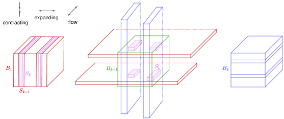
Figure 1: The geometric mechanism that allows one to prove (effective) multiple mixing, using mixing. In the middle box, the red components, coming from a condition on the past, are “perpendicular” to the blue components, which come from a condition on the future. This is the analog in the hyperbolic dynamics setting of the Markov property for random walks.

We now prove effective multiple mixing for any finite number $k$ of flow boxes. The result follows from effective mixing and the expansion/contraction (Anosov) property of the geodesic flow. Note the error term becomes bad as $k$ increases; we only use the result for small $k$.

Theorem 2.2 (Effective multiple mixing).

Fix $\delta,\epsilon,\eta>0$. Then there exists some $c>0$ with the following property. Let $X$ be any $\delta$-expander surface, and $B_{1},\ldots,B_{k}\subset T^{1}X$ be $\eta$ flow boxes. Given $t_{1},\ldots,t_{k}\geq 0$, define

$$S_{k}:=\{v:g_{t_{1}}v\in B_{1},\ldots,g_{t_{k}}v\in B_{k}\}.$$

Then

$$\mu(B)^{k}(1-\epsilon)^{k}\leq\mu\left(S_{k}\right)\leq\mu(B)^{k}(1+\epsilon)^{k}$$

whenever $t_{i}-t_{i-1}\geq c\log g$ for each $i\geq 1$. (Here $B$ is any of the flow boxes, which all have the same $\mu$ measure.)

Proof.

The upper and lower bounds follow from Lemma 2.3 and Lemma 2.4 below, respectively. ∎

An obstacle in proving 2.2 is the phenomenon of edge effects, which means the shape of some components of intersection differs from the typical shape. To deal with edge effects we enlarge/shrink our flow boxes slightly, getting upper and lower bounds in the next two lemmas.

For each $i$, we define $B_{i}^{+\epsilon}$ to be the $(1+\epsilon)\eta$ parameter flow box with the same center as $B_{i}$.

Lemma 2.3.

With the same setup as in 2.2, there exist sets $\bar{S}_{1},\ldots,\bar{S}_{k}$ such that for each $j$

1. $S_{j}\subset\bar{S}_{j}$

2. $\mu(\bar{S}_{j})\leq\mu(B^{+\epsilon})^{j}(1+\epsilon)^{j}$

3. Every component of $\bar{S}_{j}$ has full width in contracting direction, and width $e^{-t_{j}}\eta$ in expanding direction.

Proof.

We will prove the result by induction on $j$. For $j=1$, we take $\bar{S}_{j}:=S_{j}$, and the properties trivially hold.

So assume we have already constructed $\bar{S}_{j-1}$.

Now by Lemma 2.1, we can choose $c>0$ such that if $t_{j}-t_{j-1}>c\log g$, then

$$\mu\left(B_{j-1}^{+\epsilon}\cap g_{-(t_{j}-t_{j-1})}B_{j}^{+\epsilon}\right)=\mu(B^{+\epsilon})^{2}(1+O(\epsilon)),$$

where the implicit constant in $O(\cdot)$ is $\leq 1$. We have used that the $\frac{1}{\mu(B(v))}$ factor in the error term in Lemma 2.1 is comparable to $1/g$ (since $B(v)$ is fixed size, while $\mu$ is defined to be a probability measure).

Now consider $B_{j-1}^{+\epsilon}\cap g_{-(t_{j}-t_{j-1})}B_{j}^{+\epsilon}$. A bounded number of the components of this set interact with the edges of $B_{j-1}^{+\epsilon}$ or $B_{j}^{+\epsilon}$, but no such component contains a point in $g_{t_{j-1}}S_{j-1}$ (for this we need the gap $c\log g$ between times to be sufficiently large, and larger when $B^{+\epsilon}$ is only a slight enlargement of $B$; since we choose $c$ after $\epsilon$, this is not an issue). So we throw out all such components, leaving a set $F\subset B_{j-1}^{+\epsilon}\cap g_{-(t_{j}-t_{j-1})}B_{j}^{+\epsilon}$. From the expansion/contraction dynamics, we see that each component of $F$ has width $e^{-t_{j}+t_{j-1}}\eta$ in the expanding direction, full width in the contracting direction, and average width $\eta/2$ in the flow direction (by applying mixing to somewhat smaller flow boxes). It follows that there are $2e^{t_{j}-t_{j-1}}\mu(B^{+\epsilon})(1+O(\epsilon))$ components of $F$.

Now let

$$\bar{S}_{j}^{\prime}:=\left(g_{t_{j-1}}\bar{S}_{j-1}\right)\cap F,$$

$$\bar{S}_{j}:=g_{-t_{j-1}}(\bar{S}_{j}^{\prime}).$$

By the inductive hypothesis, the containment statement (i) for $\bar{S}_{j-1}$ holds, and combined with the way $F$ was defined, we have that $S_{j}\subset\bar{S}_{j}$, giving (i).

By the inductive hypothesis for (iii), we get that each component $\mathcal{C}$ of $g_{t_{j-1}}\bar{S}_{j-1}$ has full width in expanding direction, and width $e^{-t_{j}}\eta$ in contracting direction. And from the above discussion defining $F$, we know about the shapes of each of its components $\mathcal{C}^{\prime}$. It is not necessary for $\mathcal{C}$ to intersect $\mathcal{C}^{\prime}$ (because of offset in the flow direction), but if they do, then their intersection has width $e^{-(t_{j}-t_{j-1})}\eta$ in the expanding direction, and width $e^{-t_{j-1}}\eta$ in the contracting direction. See Figure 1. Applying $g_{-t_{j-1}}$ gives the desired statement (iii) about the structure of each component of $\bar{S}_{j}$.

For the measure statement (ii), observe that for each fixed component $\mathcal{C}$ of $g_{t_{j-1}}\bar{S}_{j-1}$, the average of $\mu(\mathcal{C}\cap\mathcal{C}^{\prime})$ over components $\mathcal{C}^{\prime}$ of $F$ equals

$$A_{\mathcal{C}}:=\mu(\mathcal{C})e^{-(t_{j}-t_{j-1})}/2.$$

So

$$\mu(\bar{S}_{j}) =\mu(\bar{S}_{j}^{\prime})$$

$$=\sum_{\mathcal{C}}\sum_{\mathcal{C}^{\prime}}\mu(\mathcal{C}\cap\mathcal{C}^{\prime})$$

$$=\sum_{\mathcal{C}}\operatorname{\#comp}\left(F\right)\cdot A_{\mathcal{C}}$$

$$=\sum_{\mathcal{C}}\left(2e^{t_{j}-t_{j-1}}\mu(B^{+\epsilon})\right)(1+O(\epsilon))\left(\mu(\mathcal{C})e^{-(t_{j}-t_{j-1})}/2\right)$$

$$=\mu(B^{+\epsilon})(1+O(\epsilon))\sum_{\mathcal{C}}\mu(\mathcal{C})$$

$$=\mu(B^{+\epsilon})(1+O(\epsilon))\cdot\mu(g_{t_{j-1}}\bar{S}_{j-1})$$

$$=\mu(B^{+\epsilon})(1+O(\epsilon))\cdot\mu(B^{+\epsilon})^{j-1}(1+O(\epsilon))^{j-1}\text{ \ (by induction)}$$

$$=\mu(B^{+\epsilon})^{j}(1+O(\epsilon))^{j},$$

and in the above the constant in the $O(\cdot)$ is $\leq 1$, so we get the desired result.

∎

For each $i$, we define $B_{i}^{-\epsilon}$ to be the $(1-\epsilon)\eta$ parameter flow box with the same center as $B_{i}$.

Lemma 2.4.

With the same setup as in 2.2, there exist sets $\bar{S}_{1},\ldots,S_{k}$ such that for each $j$

1. $S_{j}\supset\bar{S}_{j}$

2. $\mu(\bar{S}_{j})\geq\mu(B^{-\epsilon})^{j}(1-\epsilon)^{j}$

3. Every component of $\bar{S}_{j}$ has full width in contracting direction, and width $e^{-t_{j}}\eta$ in expanding direction.

Proof.

The proof is very similar to that of Lemma 2.3. ∎

3 Effective prime geodesic theorem

Using techniques developed by Margulis ([Mar04], also see [KH95, Section 20.6]) and effective mixing (Lemma 2.1), we prove the following effective version of the prime geodesic theorem, for surfaces with definite spectral gap. While we were writing this paper, Wu-Xue proved a related result [WX22, Theorem 2]; they use the Selberg Trace Formula, which is a fundamentally different approach.

Theorem 3.1 (Effective prime geodesic theorem).

Fix $\delta>0,s_{0}>0,\epsilon>0$. There exists a constant $c=c(\delta,s_{0},\epsilon)$ such that for any $\delta$-expander surface $X$ of genus $g$ with systole greater than $s_{0}$, and $L>c\log g$,

$$1-\epsilon\leq\frac{N(X,L)}{e^{L}/L}\leq 1+\epsilon.$$

Proof.

The only ways in which we will use the particular geometry of the surface $X$ are (i) a lower bound on systole to ensure that the flow boxes are embedded, and (ii) the rate of mixing.

Choose $\eta$ small, which for now means less than $s_{0}$; later we will send $\eta$ to $0$. For $\eta$ sufficiently small, any embedded $\eta$ flow box $B:=B(v)$ behaves very much like a product.

Now we study the sets $g_{t}B\cap B$. By Lemma 2.1,

$$\mu(g_{t}B\cap B)=\mu(B)^{2}\left(1+O(\epsilon^{\prime})+\frac{1}{\mu(B)}O(f(\eta,\epsilon^{\prime})te^{-\kappa t})\right),$$ (14)

for any choice of $\epsilon^{\prime}>0$, where $f(\eta,\epsilon^{\prime})$ is some function that does not depend on the genus of the surface or the tangent vector $v$, and $\kappa>0$ only depends on $\delta$.

We now study the geometry of each component of $g_{t}B\cap B$. If we apply geodesic flow $g_{t}$ to $B$, in the contracting horocycle direction it gets contracted by a factor of $e^{-t}$, in the flow direction its width remains unchanged, and in the expanding horocycle direction it gets expanded by a factor of $e^{t}$. This follows from the identity:

$$h^{u}_{r_{1}}\ g_{t^{\prime}}\ h^{s}_{r_{2}}\ g_{t}=g_{t}\ h^{u}_{r_{1}e^{t}}\ g_{t^{\prime}}\ h^{s}_{re^{-t}}$$

(recall that the flows are applied on the right).

It follows from this description of $g_{t}B$ that the set $g_{t}B\cap B$ consists primarily of “full components” of intersection that have thickness $\eta e^{-t}$ in the contracting direction while spanning all of $B$ in the expanding direction. By applying Lemma 2.1 to somewhat smaller flow boxes, we see that on average each full component extends close to $1/2$ way through $B$ in the $g$ direction, with the actual amount differing multiplicatively from $1/2$ by the same form of error term as in (14). There are also a number of other components that either (i) have smaller thickness in the contracting direction because they lie near the extreme parts of $B$ in the $h^{s}$ direction, or (ii) do not span all of $B$ in the expanding direction. But the number of components of types (i) and (ii) is $O(1)$, specifically the total number is bounded above by $6$.

It follows from this description and (14) that

$$\operatorname{\#comp}(g_{t}B\cap B) =\frac{\mu(g_{t}B\cap B)}{\text{average volume of each component}}+O(1)$$ (15)

$$=\frac{\mu(B)^{2}\left(1+O(\epsilon^{\prime})+\frac{1}{\mu(B)}O(f(\eta,\epsilon^{\prime})te^{-\kappa t})\right)}{\frac{1}{2}e^{-t}\mu(B)\left(1+O(\epsilon^{\prime})+\frac{1}{\mu(B)}O(f(\eta,\epsilon^{\prime})te^{-\kappa t})\right)}+O(1)$$ (16)

$$=2e^{t}\mu(B)\left(1+O(\epsilon^{\prime})+\frac{1}{\mu(B)}O(f(\eta,\epsilon^{\prime})te^{-\kappa t})\right)+O(1).$$ (17)

Now components of $g_{L}B\cap B$ correspond (up to a small additive error) to closed geodesics of length in $[L-\eta,L+\eta]$ with a distinguished time $\eta$ segment during which it passes through $B$, the number of which we denote by $N(B,L,\eta)$. This is due to Anosov Closing Lemma (Lemma 6.1, which applies at all length scales). So, combined with (17), we get

$$N(B,L,\eta)=2e^{L}\mu(B)\left(1+O(\epsilon^{\prime})+\frac{1}{\mu(B)}O(f(\eta,\epsilon^{\prime})Le^{-\kappa L})\right)+O(1).$$

To count the number $N(X,[L-\eta,L+\eta])$ of all closed geodesics of length in $[L-\eta,L+\eta]$ we apply the above results over all $B$ (which all have the same measure, denoted $\mu(B)$), giving

$$N(X, L-\eta,L+\eta)\cdot L\cdot\mu(B)$$

$$=(1+o(1))\sum_{|\gamma|\in[L-\eta,L+\eta]}\int_{t=0}^{|\gamma|}\left(\int_{T^{1}X}\chi_{\{v:\gamma(t)\in B\}}d\mu(v)\right)dt$$

$$=(1+o(1))\int_{T^{1}X}\sum_{|\gamma|\in[L-\eta,L+\eta]}\left(\int_{t=0}^{|\gamma|}\chi_{\{v:\gamma(t)\in B\}}dt\right)d\mu(v)$$

$$=(1+o(1))\int_{T^{1}X}\eta\cdot N(B,L,\eta)d\mu(v)$$

$$=(1+o(1))\eta\left[2e^{L}\mu(B)\left(1+O(\epsilon^{\prime})+\frac{1}{\mu(B)}O(f(\eta,\epsilon^{\prime})Le^{-\kappa L})\right)+O(1)\right].$$

The $1+o(1)$ error term in the above is present since the geodesics counted don’t all have length exactly $L$; the $o(\cdot)$ is as $\eta\to 0$. In the above we have summed over geodesics $\gamma$ and picked a (unit-speed) parametrization $\gamma(t)$ of each; the summands do not depend on the choice of parametrization. Rearranging gives

$$N(X, L-\eta,L+\eta)=$$ (18)

$$\frac{2\eta e^{L}}{L}(1+o(1))\left(1+O(\epsilon^{\prime})+\frac{1}{\mu(B)}O(f(\eta,\epsilon^{\prime})Le^{-\kappa L})\right)+\frac{\eta\cdot O(1)}{L\cdot\mu(B)}.$$ (19)

We then sum the above over values up to $L$, and take $\eta$ small, so that the sum of the main terms $2\eta e^{L}/L$ is well-approximated by $\int_{s_{0}}^{L}e^{t}/tdt$ (recall that we are assuming the systole is greater than $s_{0}$, hence $N(X,s_{0})=0$, which is why we can take the lower bound of integration to be $s_{0}$). This in turn is close to $e^{L}/L$ (with multiplicative error tending to $1$ as $\eta\to 0$ and any $L\to\infty$). That is

$$N(X,L)=(1+o(1))\frac{e^{L}}{L}+E_{1}+E_{2},$$ (20)

where $E_{1},E_{2}$ are error terms described below coming from integrating the error terms in (19).

We estimate the first error term as

$$E_{1} =(1+o(1))\int_{s_{0}}^{L}\frac{e^{t}}{t}\left(O(\epsilon^{\prime})+\frac{1}{\mu(B)}O(f(\eta,\epsilon^{\prime})te^{-\kappa t})\right)dt$$ (21)

$$=(1+o(1))\frac{e^{L}}{L}\cdot O(\epsilon^{\prime})+\frac{1}{\mu(B)}O(f(\eta,\epsilon^{\prime}))\frac{1}{1-\kappa}e^{(1-\kappa)L}$$ (22)

$$=(1+o(1))\frac{e^{L}}{L}\cdot O(\epsilon^{\prime})+\frac{g}{\eta^{3}}O(f(\eta,\epsilon^{\prime}))\frac{1}{1-\kappa}e^{(1-\kappa)L}.$$ (23)

The second error term is

$$E_{2} =(1+o(1))\int_{s_{0}}^{L}\frac{O(1)}{t\cdot\mu(B)}dt$$ (24)

$$\leq(1+o(1))\frac{L\cdot O(1)}{s_{0}\cdot\mu(B)}\leq(1+o(1))\frac{L\cdot O(1)g}{s_{0}\cdot\eta^{3}}.$$ (25)

Now examining (23) and (25), we see that upon taking $\eta,\epsilon^{\prime}$ small in terms of $\epsilon$, both error terms can be bounded by $\epsilon\cdot e^{L}/L$ whenever $L>c\log g$, where $c$ depends on $\epsilon$ (and $\delta$). The desired result then follows by applying these estimates in (20).

∎

4 Simple geodesics

In this section we will get an upper bound on simple geodesics $N_{simp}(X,L)$, which will allow us to prove 1.1.

4.1 An analogous probability problem

The heuristic for 1.1 derives from analysis of the “birthday problem” in probability. This involves picking $k$ objects from a collection of $n$, with replacement. The question is: how large does $k$ need to be to guarantee the chance of getting at least one object more than once is high? The transition occurs near $k=\sqrt{n}$.

In our situation we have to discretize our continuous space. We will want the resulting “boxes” to be disjoint. As a result, they will not actually cover the whole space, but rather some definite fraction of it (the “good” objects below are the ones corresponding to these disjoint boxes). In order to prove a geodesic self-intersects, it is not enough to show that it comes back close to where it has been previously. It will be enough to show that it comes back close, and at a definite angle (i.e. “transversely”).

We incorporate these two differences from the “birthday” situation into a modified probability problem, which we then solve. Our proof of the 1.1 will then be an analog of this, but in the context of hyperbolic dynamics, which, although deterministic, behaves much like a random system.

Proposition 4.1.

Fix $\alpha$ with $0<\alpha<1/3$. Let $x_{1},\ldots,x_{\ell}$ be samples from a collection $S$ of $n$ distinct objects. The samples are chosen independently, uniformly at random, and with replacement. We are additionally given a subset $G\subset S$, the “good” objects, which has size at least $\alpha\cdot n$, together with an injective map $T:G\to S$, the “transverse object” map.

Then

$$p:=\mathbb{P}[\not\exists(i,j)\text{ with }x_{j}=T(x_{i})]\to 0$$

as $n\to\infty$, provided that $\ell\succ\sqrt{n}$.

Proof.

Begin by setting $k:=\min(\ell,n^{2/3})$.

1. Let

   $$r:=\mathbb{P}\left[\#\left(\{x_{1},\ldots,x_{\lfloor(1-\alpha)k\rfloor}\}\cap G\right)\leq\alpha k/4\right].$$

   This is the probability that too few good objects are hit among the early choices.

2. Let

   $$q:=\mathbb{P}[ \#\left(\{x_{1},\ldots,x_{\lfloor(1-\alpha)k\rfloor}\}\cap G\right)>\alpha k/4$$

   $$\text{ and }x_{\lfloor(1-\alpha)k\rfloor+1},\ldots,x_{k}\not\in T(\{x_{1},\ldots,x_{\lfloor(1-\alpha)k\rfloor}\}\cap G)].$$

   This is the probability that enough good objects are hit among the early choices, and none of the later choices hits a transverse to one of the good earlier choices.

It is clear that $p\leq r+q$.

To bound $r$, we will define further probabilities based on two cases:

1. Let

   $$r_{0}:=\mathbb{P}\left[\#\{i:1\leq i\leq(1-\alpha)k,\ x_{i}\in G\}\leq\alpha k/2\right],$$

   the probability that too few of the early choices hit good objects.

2. Let

   $$r_{1}:=\mathbb{P}[ \#\{i:1\leq i\leq(1-\alpha)k,\ x_{i}\in G\}>\alpha k/2$$

   $$\text{ and }\#\left(\{x_{1},\ldots,x_{\lfloor(1-\alpha)k\rfloor}\}\cap G\right)\leq\alpha k/4],$$

   the probability that enough of the early choices hit good objects, but among these there are not enough distinct objects hit.

Note that $r\leq r_{0}+r_{1}$.

Bounding $r_{0}$: We use the second moment method. Let $X_{i}$ be the indicator random variable of the event that $x_{i}\in G$. Let $X=\sum_{i\leq(1-\alpha)k}X_{i}$, so $r_{0}=\mathbb{P}[X\leq\alpha k/2]$. We first compute the expected value of $X$. Note that $\mathbb{E}[X_{i}]=\mathbb{P}[x_{i}\in G]=\alpha$. So

$$\mathbb{E}[X]=\sum_{i\leq(1-\alpha)k}\mathbb{E}[X_{i}]=\alpha(1-\alpha)k>(2/3)\alpha k,$$

using the assumption $\alpha<1/3$.

Now we compute the second moment, using independence of the $X_{i}$:

$$\operatorname{Var}(X) =\sum_{i,j}\operatorname{Cov}(X_{i},X_{j})=\sum_{i}\operatorname{Var}(X_{i})=\sum_{i}(\alpha-\alpha^{2})=(\alpha-\alpha^{2})(1-\alpha)k$$

$$<\alpha k.$$

So by Markov’s inequality:

$$r_{0} =\mathbb{P}[X\leq\alpha k/2]\leq\mathbb{P}[|X-\mathbb{E}X|>\alpha k/6]=\mathbb{P}[(|X-\mathbb{E}X)^{2}>(\alpha k/6)^{2}]$$

$$\leq\frac{\mathbb{E}[(X-\mathbb{E}X)^{2}]}{(\alpha k/6)^{2}}=\frac{\operatorname{Var}(X)}{(\alpha k/6)^{2}}\leq\frac{\alpha k}{(\alpha k/6)^{2}}=\frac{36}{\alpha}\frac{1}{k}$$

and hence $r_{0}\to 0$ as $k\to\infty$ (which must happen when $n\to\infty$, since $k\succ\sqrt{n}$).

Bounding $r_{1}$: We use the first moment method.

Let $Y_{i,j}$ be the indicator of the event $x_{i}=x_{j}$, and $Y=\sum_{i<j}Y_{i,j}$. Note that on the event defining $r_{1}$, we must have $Y\geq\alpha k/2-\alpha k/4=\alpha k/2$, since there are least this many values of $j$ such that $x_{j}\in G$ and $x_{i}=x_{j}$ for some value of $i<j$. Then by Markov, we get

$$r_{1}\leq P[Y\geq\alpha k/2]\leq\frac{\mathbb{E}[Y]}{\alpha k/2}\leq\frac{k^{2}/n}{\alpha k/2}=\frac{2}{\alpha}\frac{k}{n},$$

which, since $k\leq n^{2/3}$ , goes to $0$ as $n\to\infty$.

Bounding $q$: Consider the conditional probability

$$q^{\prime}:=\mathbb{P}[ x_{\lfloor(1-\alpha)k\rfloor+1},\ldots,x_{k}\not\in T(\{x_{1},\ldots,x_{\lfloor(1-\alpha)k\rfloor}\}\cap G)$$

$$|\ \#\left(\{x_{1},\ldots,x_{\lfloor(1-\alpha)k\rfloor}\}\cap G\right)>\alpha k/4].$$

Note that $q\leq q^{\prime}$, so it suffices to bound $q^{\prime}$. Since $T$ is injective, the condition on the right implies that $T(\{x_{1},\ldots,x_{\lfloor(1-\alpha)k\rfloor}\}\cap G)$ has at least $\alpha k/4$ elements. So, ala the birthday problem, we compute the probability that $x_{\lfloor(1-\alpha)k\rfloor+1},\ldots,x_{k}$ all avoid these $\alpha k/4$ objects (notice that these later choices are independent of those involved in the condition), giving

$$q^{\prime} \leq\left(1-\frac{\alpha k/4}{n}\right)^{\alpha k-1}$$

$$\approx\exp\left(-\frac{\alpha k/4}{n}\right)^{\alpha k-1}$$

$$=\exp(-\Omega(k^{2}/n)),$$

(where we have used that for $n$ large, $1-\frac{\alpha k/4}{n}\geq 0$, since $k\leq n^{2/3}$). The last term goes to $0$ as $n\to\infty$, and hence so does $q$.

Completing the proof: Combing the above three cases, we get that

$$p=r+q\leq r_{0}+r_{1}+q\to 0.$$

∎

4.2 Flow boxes for proof of 1.1

Properties of the flow boxes.

Recall from Section 2 the various definitions associated with flow boxes. In what follows, we will find a collection of disjoint flow boxes that cover a definite proportion of the surface. Additionally, each box $B$ is paired with a “transverse” box $\hat{B}$ such that a geodesic crossing through $B$ and $\hat{B}$ is guaranteed to self-intersect transversely.

For each $v\in T^{1}X$, we define the rotated vector $\hat{v}:=r_{90^{\circ}}v$. If $B=B(v)$ is an $\eta$ flow box centered at $v$, we define the transverse box $\hat{B}$ to be the $\eta$ flow box centered at $\hat{v}$.

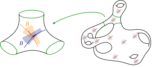
Figure 2: Transverse flow boxes guaranteeing a self-intersection. In (the unit tangent bundle over) every pair of pants, we can fit a pair of transverse flow boxes $B,\hat{B}$ of definite size. Any geodesic that lands in both $B$ and $\hat{B}$ must have a self-intersection. Thus a simple geodesic cannot hit both boxes in any such pair. We use this condition to bound the number of simple closed geodesics of length at most $L$.

Proposition 4.2.

There exists $\eta_{0},\alpha>0$, and $v_{1},\ldots,v_{2g-2}\in T^{1}X$ such that for all $\eta$ with $\eta_{0}/1000\leq\eta\leq\eta_{0}$, the $\eta$ flow boxes $B_{i}:=B(v_{i})$ and $\hat{B}_{i}:=B(\hat{v}_{i})$ satisfy:

1. $\mu\left(\cup_{i}B_{i}\right)>\alpha.$

2. The $B_{1},\ldots,B_{2g-2},\hat{B}_{1},\ldots,\hat{B}_{2g-2}$ are pairwise disjoint

3. If $t_{1},t_{2}\in\mathbb{R}$ and $v$ is such that $g_{t_{1}}v\in B_{i}$ and $g_{t_{2}}v\in\hat{B}_{i}$, then the geodesic $t\mapsto g_{t}v$ has a transverse self-intersection

4. “full box separated” i.e. for any $w\in T^{1}X-\bigcup_{i=1}^{2g-2}\hat{B}_{i}^{+}$, the $\eta$ flow box $B(w)$ satisfies $B(w)\subset T^{1}X-\bigcup_{i=1}^{2g-2}\hat{B}_{i}$.

Here $\eta_{0},\alpha$ are independent of $g$, but do depend on the systole lower bound $s_{0}$ that $X$ is assumed to satisfy.

The proof of this proposition will depend on the following observation giving that any surface has many points where the injectivity radius is bounded below by a uniform constant.

Lemma 4.3.

There is a universal constant $r_{0}>0$ so that any hyperbolic pair of pants $P$ with geodesic boundary contains an embedded ball of radius $r_{0}$.

Proof.

We first decompose our pair of pants $P$ into two isometric right-angled hexagons. Let $H$ be one of these hexagons. By the Gauss-Bonnet formula, the area of a $H$ is $\pi$. We can cut $H$ into the union of 4 triangles. See Figure 3. One of these triangles, denoted $T$, must have area at least $\pi/4$. Every hyperbolic triangle of area at least $A$ contains an embedded ball of radius $r(A)$, for some function $r$. This follows from compactness of the set of isometry types of such triangles (allowing ideal vertices), since hyperbolic triangles are determined up to isometry by their angles, and the area bound implies the angle sum is bounded from above away from $\pi$. So we take $r_{0}=r(\pi/4)$.

∎

Figure 3: Every right-angled hyperbolic hexagon contains a disc of definite area.

With this, we can prove the proposition.

Proof of Proposition 4.2.

Let $X$ be any hyperbolic surface of genus $g$. Take a pants decomposition $P_{1},\dots,P_{2g-2}$ of $X$. By Lemma 4.3, we can fit a disc $D_{i}$ of radius $r_{0}$ inside each pair of pants $P_{i}$. As the pairs of pants have disjoint interiors, these discs will be pairwise disjoint, as well.

We will find our collection of flow boxes $B_{1},\dots,B_{2g-2},\hat{B}_{1},\dots,\hat{B}_{2g-2}$ in the unit tangent bundle above these discs. Let $\pi:T^{1}X\to X$ be the usual projection. We observe that there is some constant $\eta_{0}$ so that for all $\eta<\eta_{0}$, if $B$ is an $\eta$ flow box, and $\pi(B)\subset D_{i}$, then $B$ is embedded in $T^{1}X$. In fact, for all $\eta$ small enough, a lift of $B$ will be embedded in the universal cover $T^{1}\mathbb{H}^{2}$, and since $D_{i}$ is embedded in $X$, then $B$ will be embedded in $T^{1}X$.

Fix such an $\eta_{0}$. Make it smaller if necessary, so that $\eta_{0}<r_{0}/100$ (and note that we might retroactively make $\eta_{0}$ smaller again later in the proof). We will show that the proposition holds for any $\eta$ with $\eta_{0}/1000<\eta<\eta_{0}$.

Suppose $p_{i}$ is the center of $D_{i}$. Let $v_{i}$ be any vector in $T^{1}_{p_{i}}X$. Then we claim that the $\eta$ flow box $B_{i}=B(v_{i})$ centered at $v_{i}$ is embedded in $T^{1}X$. In fact, let $w\in B_{i}$. Then to get from $\pi(v_{i})=p_{i}$ to $\pi(w)$, we must follow a leaf of the stable horocycle foliation, then a geodesic segment, then a leaf of the unstable horocycle foliation, and each segment we follow has length at most $\eta$. Thus, the distance from $p_{i}$ to $\pi(w)$ is at most $3\eta$. As $3\eta<r_{0}$ by definition, $\pi(w)\in D_{i}$. So $\pi(B_{i})\subset D_{i}$, and by the above discussion, $B_{i}$ must be embedded.

Note that if we fix $\eta_{0}$, and if $\eta>\eta_{0}/1000$, say, then there will be some $\alpha$ depending on $\eta$ so that

$$\mu(B_{i})>\alpha\mu(T^{1}P_{i})$$

where $T^{1}P_{i}=\pi^{-1}P_{i}$ is the unit tangent bundle of $P_{i}$ inside $X$. As there is a box above each pair of pants, we see that

$$\mu\left(\bigcup_{i=1}^{2g-2}B_{i}\right)>\alpha$$

Thus, our collection of boxes $B_{1},\dots,B_{2g-2}$ satisfies part (i).

Next, let $\hat{v}_{i}=r_{\pi/2}v_{i}$, that is, the tangent vector making an angle of $\pi/2$ with $v_{i}$. Recall $\hat{B}_{i}=B(\hat{v}_{i})$. Again making $\eta_{0}$ smaller if necessary, we claim that $B_{i}$ and $\hat{B}_{i}$ are disjoint. In fact, choose any $PSL(2,\mathbb{R})$-invariant Riemannian metric on $T^{1}\mathbb{H}^{2}$. This induces a Riemannian metric on $T^{1}X$. Then as $\eta_{0}$ goes to 0, for any $\eta<\eta_{0}$, the diameter of the $\eta$ flow boxes $B_{i}$ and $\hat{B}_{i}$ also goes to zero. Thus, $B_{i}$ must be disjoint from $\hat{B}_{i}$ for all $\eta$ small enough. This establishes (ii).

Moreover, if $w\in B_{i}$ and $\hat{w}\in\hat{B}_{i}$, then $w$ and $\hat{w}$ also get arbitrarily close to $v_{i}$ and $\hat{v}_{i}$, respectively. In fact, let $\gamma_{v_{i}}$ and $\gamma_{\hat{v}_{i}}$ be the complete geodesics tangent to $v_{i}$ and $\hat{v}_{i}$. Then $\gamma_{v_{i}}$ and $\gamma_{\hat{v}_{i}}$ intersect at an angle of $\pi/2$. This means that the geodesics $\gamma_{w}$ and $\gamma_{\hat{w}}$ tangent to $w$ and $\hat{w}$, must also intersect transversely for $\eta_{0}$ small enough, establishing (iii).

Lastly, we will show that the flow boxes are “full box separated”. Recall that $\hat{B}_{i}^{+}$ is the $3\eta$ flow box centered around $\hat{v}_{i}$. Since we chose $\eta_{0}<r/1000$, the box $\hat{B}_{i}^{+}$ is still embedded in $T^{1}X$. Let $w\in T^{1}X-\bigcup_{i=1}^{2g-2}\hat{B}_{i}^{+}$. We will show that $B(w)$ is disjoint from $\bigcup_{i=1}^{2g-2}\hat{B}_{i}$. In fact, let $w^{\prime}\in B(w)$. Suppose $w^{\prime}\in\hat{B}_{i}$ for some $i$. If the flow boxes were, in fact, Euclidean boxes, then the fact that $w^{\prime}\in B(w)\cap\hat{B}_{i}$ and that these are both $\eta$ flow boxes would mean that $w$ was in the $2\eta$ flow box around $\hat{v}_{i}$. But as $\eta$ tends to 0, the flow boxes get close to Euclidean boxes. So choosing $\eta_{0}$ smaller, if needed, $w^{\prime}\in B(w)\cap\hat{B}_{i}$ implies that $w$ is in the $3\eta$ flow box about $\hat{v}_{i}$. In other words, $w\in\hat{B}_{i}^{+}$, which contradicts our assumptions. Thus, our collection of flow boxes satisfies condition (iv). ∎

4.3 Bound on measure of $S$

Fix an $\eta$ flow box $B\subset T^{1}X$. We will focus for now on bounding from above the number of simple closed geodesics that intersect $B$.

Let

$$S:=\{v\in B:t\mapsto g_{t}v\text{ does not self-intersect}\},$$

i.e. the set of all vectors in $B$ tangent to (not necessarily closed) simple geodesics.

We need a bound on the measure of this set, and then we will add the condition that the arcs return to $B$ at time $L$, since we are interested in counting closed geodesics. However, having bounds on measures is not quite enough, since simple closed geodesics will correspond to certain connected components, and we need to make sure that there are not too many of these. To address this, we will work with a modified larger set $\bar{S}$, with the property that every vector in its complement corresponds to an arc with a “robust self-intersection”, which must occur before a certain time. We then bound the measure of $\bar{S}$.

The existence and properties of this set $\bar{S}$ are the content of the next lemma.

Lemma 4.4.

For any $\epsilon>0$, there exists $c$ with the following property. For any $k$ positive integer, there exists a set $\bar{S}\subset B$, such that

1. $\bar{S}\supset S$,

2. For any $u\in B-\bar{S}$, there exists some $\eta$ flow box $B_{0}$ and $t_{1},t_{2}\in[0,kc\log g]$ such that $g_{t_{1}}u\in B_{0}^{++}$ and $g_{t_{2}}u\in\hat{B}^{-}_{0}$ (which implies the geodesic segment through $u$ has a “robust self-intersection”),

3. $$\mu(\bar{S})\leq\mu(B)\left(\epsilon+O(1/k)+O(k/g)+\left\{1-\frac{1}{O(1)}k\mu(B)\right\}^{\alpha k}\right).$$

We will construct $\bar{S}$ as a union of sets $R$ and $Q_{k}$ corresponding to different behavior with respect to a collection of flow boxes that we use to probe simplicity, discussed in Section 4.2.

Collection of flow boxes.

We fix $\{B_{\nu}\}_{\nu=1}^{2g-2}=\{B_{1},\ldots,B_{2g-2}\}$ a collection of $\eta$ flow boxes in $T^{1}X$ given by 4.2, where $\eta=\eta_{0}/27$, for the $\eta_{0}$ given by that proposition.

Discrete set of times.

We pick times at which to sample the geodesic segments. Let $t_{1},t_{2},\ldots$ such $t_{i+1}-t_{i}=c\log g$ (where $c$ will be chosen large later, as mentioned in the lemmas below; it is related to mixing time for geodesic flow, and will depend on an error parameter $\epsilon$). The earlier and later times among these will play somewhat different roles when we study self-intersections.

4.3.1 $R$: Vectors that hit too few flow boxes $\{B_{\nu}\}$

For any positive integer $k$, let

$$R=R(k):=\Big{\{}v\in B:\#\{\nu:\exists j\leq(1-\alpha)k\text{ such that }g_{t_{j}}v\in B_{\nu}\}<\alpha k/4\Big{\}},$$

i.e. $R$ consists of vectors that do not hit at least $\frac{\alpha}{4}k$ distinct elements of $\{B_{\nu}\}$ among times $t_{1},\ldots,t_{\lfloor(1-\alpha)k\rfloor}$.

Lemma 4.5.

For any $\epsilon>0$, there exists $c$ such that

$$\mu(R)\leq\mu(B)\left(\epsilon+O(1/k)+O(k/g)\right).$$

Proof.

We have $R=R_{0}\sqcup R_{1}$ for the sets $R_{0},R_{1}$ defined below. The desired bound is just the sum of the bounds from Lemma 4.6 for $R_{0}$ and Lemma 4.7 for $R_{1}$. ∎

Decomposition $R=R_{0}\sqcup R_{1}$.

We define a set of starting vectors that visit our collection of flow boxes too few times:

$$R_{0}=R_{0}(k):=\left\{v\in B:\#\{i:i\leq(1-\alpha)k,\ \ g_{t_{i}}v\in\cup_{\nu}B_{\nu}\}\leq(\alpha/2)k\right\}.$$

The complementary set consists of vectors that hit flows boxes at enough times, but that still hit too few distinct flow boxes:

$$R_{1}:=R-R_{0}.$$

Lemma 4.6.

For any $\epsilon>0$, there exists $c$ such that

$$\mu(R_{0})\leq\mu(B)\left(\epsilon+O(1/k)\right).$$

Proof.

For each $i$ with $i\leq(1-\alpha)k$, and each $\nu$, define $X_{i\nu}:B\to\mathbb{R}$ by

$$X_{i\nu}(v)=\begin{cases}\begin{matrix}1&\text{ if }g_{t_{i}}v\in B_{\nu}\\ 0&\text{otherwise.}\end{matrix}\end{cases}$$

Since the boxes $B_{\nu}$ are all disjoint, we have that

$$X_{i}:=\sum_{\nu}X_{i\nu}$$

is either 0 or 1 for all $i$, and determines whether $g_{t_{i}}v$ hits any of the boxes $B_{1},\dots,B_{2g-2}$ at time $t_{i}$. Thus, if we set

$$X=\sum_{i\leq(1-\alpha)k}X_{i},$$

then $X(v)$ is the number of times $i$ for which $g_{t_{i}}v$ hits boxes $B_{1},\dots,B_{2g-2}$. So we wish to show

$$\mu(\left\{v:X(v)\leq(\alpha/2)k\right\})=\mu(B)\left(O(\epsilon)+O(1/k)\right).$$

We will use the second moment method. For this, we will first estimate $\frac{1}{\mu(B)}\int_{B}Xd\mu$ and $\frac{1}{\mu(B)}\int_{B}X^{2}d\mu$. To estimate $\int_{B}X$, we just need to estimate $\int_{B}X_{i\nu}$ for each $i,\nu$. We have

$$\int_{B}X_{i\nu} =\mu(\{v\in B:g_{t_{i}}v\in B_{\nu}\})$$

$$=\mu(B\cap g_{-t_{i}}(B_{\nu}))$$

$$=\mu(B_{\nu})^{2}\left(1+O(\epsilon)\right),$$

for $c$ sufficiently large, where the last line is due to effective mixing (Lemma 2.1 or $k=2$ case of 2.2).

Then summing gives

$$\frac{1}{\mu(B)}\int_{B}X =\frac{1}{\mu(B)}\sum_{i\leq(1-\alpha)k}\sum_{\nu}\int_{B}X_{i\nu}=\sum_{i\leq(1-\alpha)k}\sum_{\nu}\mu(B_{\nu})\left(1+O(\epsilon)\right)$$ (26)

$$=(1-\alpha)k\alpha(1+O(\epsilon)).$$ (27)

Now we must estimate $\frac{1}{\mu(B)}\int_{B}X^{2}$. Writing $X=\sum_{i}X_{i}$, we see that

$$X^{2}=\sum_{i}X_{i}+\sum_{i\neq j}X_{i}X_{j}$$

where we use that $X_{i}$ is always either 0 or 1, and so $(X_{i})^{2}=X_{i}$. To estimate $\int_{B}X_{i}X_{j}$, we use that $X_{i}=\sum_{\nu}X_{i\nu}$, and so $X_{i}X_{j}=\sum_{\nu,\nu^{\prime}}X_{i\nu}X_{j\nu^{\prime}}$. Now for $i\neq j$

$$\int_{B}X_{i\nu}X_{j\nu^{\prime}} =\mu(\{v\in B:g_{t_{i}}v\in B_{\nu},\ g_{t_{j}}v\in B_{\nu^{\prime}}\})$$

$$=\mu(B\cap g_{-t_{i}}B_{\nu}\cap g_{-t_{j}}B_{\nu^{\prime}})$$

$$=\mu(B)\mu(B_{\nu})\mu(B_{\nu^{\prime}})\left(1+O(\epsilon)\right)^{3},$$

for $c$ sufficiently large, where the last line comes from effective 3-mixing, i.e. the $k=3$ case of 2.2.

For $\epsilon$ small enough, $\left(1+O(\epsilon)\right)^{3}=\left(1+O(\epsilon)\right)$. Thus, summing over all $\nu,\nu^{\prime}$, we get for $i\neq j$

$$\frac{1}{\mu(B)}\int_{B}X_{i}X_{j}=\alpha^{2}\left(1+O(\epsilon)\right).$$

Using this, (27), and the fact that there are at most $(1-\alpha)^{2}k^{2}$ pairs of $i\neq j$, we see that

$$\frac{1}{\mu(B)}\int_{B}X^{2} =\frac{1}{\mu(B)}\int_{B}X+\sum_{i\neq j}\frac{1}{\mu(B)}\int_{B}X_{i}X_{j}$$ (28)

$$\leq(1-\alpha)k\alpha(1+O(\epsilon))+(1-\alpha)^{2}k^{2}\alpha^{2}(1+O(\epsilon))$$ (29)

Combining the first and second moment bounds, (27) and (29), we estimate

$$\frac{1}{\mu(B)} \int_{B}(X-(1-\alpha)\alpha k)^{2}=\frac{1}{\mu(B)}\left(\int_{B}X^{2}-2(1-\alpha)\alpha k\int_{B}X+\mu(B)(1-\alpha)^{2}\alpha^{2}k^{2}\right)$$

$$\leq(1+O(\epsilon))\left((1-\alpha)k\alpha+(1-\alpha)^{2}k^{2}\alpha^{2}-2(1-\alpha)^{2}(k\alpha)^{2}+(1-\alpha)^{2}k^{2}\alpha^{2}\right)$$

$$=O(k)+O(\epsilon k^{2}).$$

Using this, we apply a Chebyshev bound. Note that since we can assume that $\alpha$ is small, if $X\leq(\alpha/2)k$ then $|X-(1-\alpha)\alpha k|\geq(1/3)\alpha k$. So:

$$\frac{1}{\mu(B)}\cdot\mu\left(\{v:X(v)\leq(\alpha/2)k\}\right) \leq\frac{1}{\mu(B)}\cdot\mu\left(\{v:(X(v)-(1-\alpha)\alpha k)^{2}\geq(\alpha k/3)^{2}\}\right)$$

$$\leq\frac{\frac{1}{\mu(B)}\int_{B}(X-(1-\alpha)\alpha k)^{2}}{(\alpha k/3)^{2}}$$

$$\leq\frac{O(k)+O(\epsilon k^{2})}{(\alpha k/3)^{2}}$$

$$\leq O(1/k)+O(\epsilon),$$

which gives the desired result.

∎

Lemma 4.7.

There exists $c$ such that

$$\mu(R_{1})\leq\mu(B)O(k/g).$$

Proof.

We will measure collisions with the function $Y_{i,j}:B\to\mathbb{R}$ given by

$$Y_{i,j}(v)=\begin{cases}1\quad\text{if }\exists\nu\text{ such that }g_{t_{i}}v,g_{t_{j}}v\in B_{\nu}\\ 0\quad\text{otherwise}.\end{cases}$$

Let $Y:=\sum_{i<j\leq(1-\alpha)k}Y_{i,j}$. Note that if $v\in R_{1}$ then $Y(v)\geq\alpha k/2-\alpha k/4=\alpha k/2$ since there must be at least this many values of $j<(1-\alpha)k$ such that $g_{t_{j}}v$ is in some flow box $B_{\nu}$ and there exists some $i<j$ for which $g_{t_{i}}v$ is in the same flow box. Thus

$$\mu(R_{1})\leq\mu(\{v\in B:Y(v)\geq\alpha k/2\}).$$ (30)

We now use the first moment method to bound the right hand term above. Define $Y_{i,j,\nu}:B\to\mathbb{R}$ by

$$Y_{i,j,\nu}(v)=\begin{cases}1\quad\text{if }g_{t_{i}}v,g_{t_{j}}v\in B_{\nu}\\ 0\quad\text{otherwise},\end{cases}$$

and note that, by disjointness of the $B_{\nu}$, we have $Y_{i,j}=\sum_{\nu}Y_{i,j,\nu}$. Hence by effective multiple mixing, 2.2,

$$\int_{B}Y_{i,j} =\sum_{\nu}\int_{B}Y_{i,j,\nu}=\sum_{\nu}\mu(B\cap g_{-t_{i}}B_{\nu}\cap g_{-t_{j}}B_{\nu})$$

$$=\sum_{\nu}\mu(B)\mu(B_{\nu})^{2}O(1)$$

$$=\alpha\mu(B)^{2}O(1).$$

Then

$$\int_{B}Y=\sum_{i<j\leq(1-\alpha)k}\int_{B}Y_{i,j}\leq\left((1-\alpha)k\right)^{2}\left(\alpha\mu(B)^{2}O(1)\right)\leq O(1)k^{2}\mu(B)^{2}.$$

Using this we apply a Markov bound:

$$\mu(\{v\in B:Y(v)\geq\alpha k/2\})\leq\frac{\int_{B}Y}{\alpha k/2}\leq\frac{O(1)k^{2}\mu(B)^{2}}{\alpha k/2}=\mu(B)O(k/g),$$

since $\mu(B)=O(1/g)$. Combining with (30) gives the desired result.

∎

4.3.2 $Q$: Vectors that hit enough flow boxes $\{B_{\nu}\}$

We now consider those vectors that intersect enough flow boxes, and then consider decreasing subsets that avoid progressively more types of self-intersection. We show that the measure of these subsets decreases in a definite way.

We fix a positive integer $k$. Then let

$$Q^{=}:= B-R$$

$$= \Big{\{}v\in B:\ \exists B_{\nu_{1}(v)},\ldots,B_{\nu_{\lfloor(\alpha/4)k\rfloor}(v)}\in\{B_{\nu}\}\text{ distinct s.t. }\forall i\leq\frac{\alpha}{4}k,$$

$$\text{ \ \ \ }\exists j\leq(1-\alpha)k\text{ s.t. }g_{t_{j}}v\in B_{\nu_{i}(v)}\Big{\}},$$

i.e. $Q^{=}$ consists of vectors that hit at least $\frac{\alpha}{4}k$ distinct elements of $\{B_{\nu}\}$ among times $t_{1},\ldots,t_{\lfloor(1-\alpha)k\rfloor}$, which we label $B_{\nu_{1}(v)},\ldots,B_{\nu_{\lfloor(\alpha/4)k\rfloor}(v)}$.

To deal with “edge effect components”, we will consider similar sets defined with respect to flow boxes of slightly different size (as in proof of 2.2). Let $Q^{+}\subset B^{+}$ be the corresponding set for the $\{B_{\nu}^{+}\}$, i.e.

$$Q^{+}:= \Big{\{}v\in B^{+}:\ \exists B^{+}_{\nu^{+}_{1}(v)},\ldots,B^{+}_{\nu^{+}_{\lfloor(\alpha/4)k\rfloor}(v)}\in\{B^{+}_{\nu}\}\text{ distinct s.t. }\forall i\leq\frac{\alpha}{4}k,$$

$$\text{ \ \ \ }\exists j\leq(1-\alpha)k\text{ s.t. }g_{t_{j}}v\in B^{+}_{\nu^{+}_{i}(v)}\Big{\}}.$$

Note that $Q^{=}\subset Q^{+}$. We then define $Q$ to be the union of components of $Q^{+}$ that intersect $Q^{=}$ i.e.

$$Q:=\bigcup\{\mathcal{C}\text{ component of }Q^{+}:\mathcal{C}\cap Q^{=}\neq\emptyset\}.$$

Note that $Q^{=}\subset Q\subset Q^{+}$.

In the the below lemma we construct progressively smaller sets $Q_{j}$ by imposing further conditions. Part (iii) corresponds to the fact that $Q_{j}$ is defined in terms of conditions on the behavior of vectors under geodesic flow only up to time $t_{j}$.

Lemma 4.8.

For each $k\geq 0$, there exist sets

$$Q_{\lceil(1-\alpha)k\rceil-1}\supset Q_{\lceil(1-\alpha)k\rceil}\supset\cdots\supset Q_{k}$$

where $Q_{\lceil(1-\alpha)k\rceil-1}:=Q$, and such that for each $j=\lceil(1-\alpha)k\rceil,\ldots,k$:

1. $S\cap Q=S\cap Q_{j}$. Furthermore, for any $u\in Q_{j-1}-Q_{j}$, there exists some $B_{\nu}$ and $j^{\prime}\leq k$ such that $g_{t_{j^{\prime}}}u\in B_{\nu}^{++}$ and $g_{t_{j}}u\in\hat{B}^{-}_{\nu}$ (which implies the geodesic segment through $u$ has a “robust self-intersection”).

2. $\mu(Q_{j})\leq\mu(B)\left\{1-\frac{1}{O(1)}k\mu(B)\right\}^{j-\lceil(1-\alpha)k\rceil}$, where $\{x\}$ denotes $\max(x,0)$.

3. $Q_{j}$ is a union of subboxes that are full width in the contracting direction, and have width $\geq e^{-t_{j}}\eta$ in the expanding direction.

Proof.

We will inductively construct the sets, verifying the listed properties along the way.

For the base case, set $Q_{\lceil(1-\alpha)k\rceil}:=Q$. Then properties (i) and (ii) are immediate. For (iii), note that because of the space between the $B_{\nu}$ and $B_{\nu}^{+}$, any component of $Q^{+}$ that intersects $Q^{=}$ is contracting width full and expanding width $\geq e^{-t_{\lceil(1-\alpha)k\rceil}}\eta$.

Suppose we have constructed $Q_{j}$ with the desired properties; we will now construct $Q_{j+1}$.

Note that any $v\in Q_{j}$ is also in $Q$, hence also in $Q^{+}$, which means there exist $B^{+}_{\nu^{+}_{1}(v)},\ldots,B^{+}_{\nu^{+}_{\lfloor(\alpha/4)k\rfloor}(v)}\in\{B^{+}_{\nu}\}$ distinct such that for each $i\leq\frac{\alpha}{4}k$ there exists a $j\leq(1-\alpha)k\text{ such that }g_{t_{j}}v\in B^{+}_{\nu_{i}(v)}$. Note that any $v^{\prime}$ sufficiently close to $v$ will satisfy this same property with the boxes enlarged, i.e. $g_{t_{j}}v^{\prime}\in B^{++}_{\nu_{i}(v)}$ (for the same $i$’s and $j$’s as for $v$). By a simple 3-times covering lemma argument, we can cover at least $1/1000$ of the measure of $Q_{j}$ by a union of a set $\mathcal{P}$ of disjoint subboxes that have full width in the contracting direction and width at least $e^{-t_{j}}\eta$ in the expanding direction, and such that for each $P\in\mathcal{P}$ we can take a common value of $\nu_{1}(P),\ldots,\nu_{\lfloor(\alpha/)4k\rfloor}(P)$ that works for all $v^{\prime}\in P$. That is, for each $i$ there exists a $j\leq(1-\alpha)k$ such that $g_{t_{j}}v^{\prime}\in B^{++}_{\nu_{i}(P)}$ for all $v^{\prime}\in P$.

With this definition of $\mathcal{P}$, we then define

$$Q^{=}_{j+1}:=Q_{j}-\bigcup_{P\in\mathcal{P}}\bigcup_{\ell=1}^{\lceil\frac{\alpha}{4}k\rceil}P\cap g_{-t_{j+1}}\hat{B}_{\nu_{\ell}(P)},$$

$$Q^{-}_{j+1}:=Q_{j}-\bigcup_{P\in\mathcal{P}}\bigcup_{\ell=1}^{\lceil\frac{\alpha}{4}k\rceil}P\cap g_{-t_{j+1}}\hat{B}_{\nu_{\ell}(P)}^{-}.$$

Note that $Q^{=}_{j+1}\subset Q^{-}_{j+1}$. Finally, define $Q_{j+1}$ to be the union of components of $Q^{-}_{j+1}$ that intersect $Q^{=}_{j+1}$. Note that $Q^{=}_{j+1}\subset Q_{j+1}\subset Q^{-}_{j+1}$.

We now verify the desired properties of $Q_{j+1}$ (assuming the properties for $Q_{j}$).

1. For Property (i), we first prove the second more specific statement. We will prove the condition holds for any tangent vector $u$ in $Q_{j}-Q_{j+1}^{=}$, from which the desired result follows since $Q_{j+1}^{=}\subset Q_{j+1}$. Note that for any such $u$, there is some $P\in\mathcal{P}$ and $\ell$ such that $u\in P$, and $g_{-t_{j+1}}\hat{B}_{\nu_{\ell}(P)}$, i.e. $g_{t_{j+1}}u\in\hat{B}_{\nu_{\ell}(P)}$. On the other hand, by definition of $\nu_{\ell}(P)$, there exists $j^{\prime}$ such that $g_{t_{j^{\prime}}}u\in B^{++}_{\nu_{\ell}(P)}$. This is the desired statement.

   Next we show that

   $$S\cap Q_{j}=S\cap Q_{j+1}.$$

   In fact, by the above, for any $u\in Q_{j}-Q_{j+1}$, its geodesic segment hits both $B^{++}_{\nu_{\ell}(P)},\hat{B}_{\nu_{\ell}(P)}$, which forces it to have a self-intersection (by 4.2, (iii)), and hence cannot lie in $S$. Iterating the equality over $j$ gives $S\cap Q=S\cap Q_{j+1}.$

2. Property (ii) we will prove by bounding $\mu(Q^{-}_{j+1})$ using disjointness of $\hat{B}_{\nu_{\ell}(P)}^{-},\hat{B}_{\nu_{\ell^{\prime}}(P)}^{-}$.

   First note that for any $P\in\mathcal{P}$, by Lemma 4.10 (for which the width hypothesis holds by property (iii) for $Q_{j}$, which we know by induction):

   $$\mu\left(P\cap g_{-t_{j+1}}\hat{B}_{\nu_{\ell}(P)}^{-}\right)\geq(1-\epsilon)\mu(P)\mu(B_{\nu_{\ell}(P)}^{-})\geq\frac{1}{O(1)}\mu(P)\mu(B),$$ (31)

   where here, and in the below computation, $O(1)$ is positive.

   Then

   $$\mu(Q_{j+1}) \leq\mu(Q^{-}_{j+1})=\mu\left(Q_{j}-\bigcup_{P\in\mathcal{P}}\bigcup_{\ell\leq\frac{\alpha}{4}k}P\cap g_{-t_{j+1}}\hat{B}_{\nu_{\ell}(P)}^{-}\right)$$

   $$\leq\mu(Q_{j})-\sum_{P\in\mathcal{P}}\sum_{\ell\leq\frac{\alpha}{4}k}\mu\left(P\cap g_{-t_{j+1}}\hat{B}_{\nu_{\ell}(P)}^{-}\right)$$ (by disjointness)

   $$\leq\mu(Q_{j})-\sum_{P\in\mathcal{P}}\sum_{\ell\leq\frac{\alpha}{4}k}\frac{1}{O(1)}\mu(P)\mu(B)$$ (by (31))

   $$\leq\mu(Q_{j})-\mu(B)\cdot\frac{\alpha}{4}k\cdot\frac{1}{O(1)}\sum_{P\in\mathcal{P}}\mu(P)$$

   $$\leq\mu(Q_{j})-\mu(B)\cdot\frac{\alpha}{4}k\cdot\frac{1}{O(1)}\cdot\frac{\mu(Q_{j})}{1000} \text{ (using property of }\mathcal{P})$$

   $$\leq\mu(Q_{j})\left[1-\frac{1}{O(1)}\mu(B)k\right]$$

   $$\leq\mu(B)\left[1-\frac{1}{O(1)}\mu(B)k\right]^{j-\lceil(1-\alpha)k\rceil}\left[1-\frac{1}{O(1)}\mu(B)k\right] \text{ (by inductive hyp. for }Q_{j})$$

   $$\leq\mu(B)\left[1-\frac{1}{O(1)}\mu(B)k\right]^{j+1-\lceil(1-\alpha)k\rceil}.$$

3. Property (iii) follows from the “full box separated” property of our flow boxes; edge effects are avoided by only taking the components that intersect $Q^{=}_{j+1}$.

∎

4.4 Proof of Lemma 4.4

Proof of Lemma 4.4.

We define

$$\bar{S}:=R\cup Q_{k},$$

where $R=R(k)$ was defined in Section 4.3.1, and $Q_{k}$ in Lemma 4.8.

1. For (i), note that by definition of $Q^{=}$, we have $B=R\cup Q^{=}$, and since $Q\supset Q^{=}$, we also have $B=R\cup Q$. By applying Lemma 4.8 (i) we then see that $S\subset R\cup Q_{k}=\bar{S}$.

2. For (ii), note that any $u\in B-\bar{S}$ is in some $Q_{j}-Q_{j+1}$ (it is “removed” at some stage in the process of paring down the $Q_{j}$). By the second part of Lemma 4.8 (i), this means that $u$ satisfies the desired property.

3. For (iii), we have

   $$\mu(\bar{S}) \leq\mu(R)+\mu(Q_{k}),$$

   and then we use the measure estimates Lemma 4.5 and Lemma 4.8 (ii).

∎

4.5 Lemmas on intersections with subboxes

Here we prove lemmas concerning the intersection of a subbox with the preimage of a full box under geodesic flow for a sufficiently large time. These are used in Section 4.3.2 and Section 4.6. While we do not have effective mixing for arbitrary subboxes, under certain conditions involving their shape, we can get control using effective mixing of the full flow boxes that contain them.

The first lemma concerns a subbox that is full in the expanding direction; this condition corresponds to conditioning only on past behavior. This lemma is then used in the proof of Lemma 4.10, which concerns a subbox that is full in the contracting direction and has width in the expanding direction controlled from below.

Lemma 4.9.

For any $\epsilon>0$, there exists $c$ satisfying the following. Let $B_{0},B_{1}$ be $\eta$ flow boxes. Let $P\subset B_{0}$ be a subbox that is full width in the expanding direction. Then for $T\geq c\log g$,

$$\mu(P\cap g_{-T}B_{1})\geq(1-\epsilon)\mu(P)\mu(B_{1}).$$

Proof.

Recall that $B_{i}^{-}$ is a flow box with the same center as $B_{i}$, but with width $\eta/3$ in each direction. Let $F$ be the union of components of $B_{0}\cap g_{-T}B_{1}$ that also intersect $B_{0}^{-}\cap g_{-T}(B_{1}^{-})$. Clearly $F\subset B_{0}\cap g_{-T}B_{1}$. Since this construction removes components with edge effects, we get that the components of $F$ are all full in the contracting direction (as subsets of $B_{0}$), and width $\geq e^{-T}\eta$ in the expanding direction.

By effective mixing, Lemma 2.1, we can choose $c>0$ such that if $t_{k}-t_{k-1}>c\log g$, then (noting that the $\frac{1}{\mu(B_{i})}$ factor in the error term is comparable to $1/g$, since $B_{i}$ is fixed size, but $\mu$ is defined to be a probability measure):

$$\mu(B_{0}\cap g_{-T}B_{1})\geq\mu(B_{0})\mu(B_{1})(1+O(\epsilon)).$$

It also follows from effective mixing, Lemma 2.1 applied to smaller flow boxes, that the components of $B_{0}\cap g_{-T}B_{1}$ have average width in the flow direction within an $1+O(\epsilon)$ factor of $\eta/2$. Since $F$ is obtained from this set by removing a bounded number of components, the same measure bound and average flow width statements of components are also true of $F$.

From the geometry of $P$ and components of $F$, we then see that, as in proof of Lemma 2.3,

$$\mu(P\cap F) =\frac{1}{\mu(B_{0})}\mu(P)\mu(F)(1+O(\epsilon))$$

$$\geq\frac{1}{\mu(B_{0})}\mu(P)\mu(B_{0})\mu(B_{1})(1+O(\epsilon))=\mu(P)\mu(B_{1})(1+O(\epsilon)),$$

from which the desired bound follows.

∎

Lemma 4.10.

For any $\epsilon,\eta>0$, there exists $c$ satisfying the following. Let $B,B^{\prime}$ be $\eta$ flow boxes, and $t\geq 0$. Let $P\subset B$ be a subbox that is full width in the contracting direction, and width $e^{-t}\eta$ in the expanding direction. Then if $T\geq t+c\log g$,

$$\mu(P\cap g_{-T}B^{\prime})\geq(1-\epsilon)\mu(P)\mu(B^{\prime}).$$

Proof.

Note that $g_{t}(P)$ has expanding width exactly $\eta$, contracting width $e^{-t}\eta$ (and flow direction width is unchanged). Take an $\eta$ flow box $B_{int}$ centered at the center of $g_{t}(P^{\prime})$.

Now we apply Lemma 4.9 with $B_{0}=B_{int}$, $B_{1}=B^{\prime}$, subbox $g_{t}(P)\subset B_{0}$, and time $c\log g$. We get that

$$\mu(g_{t}(P)\cap g_{-c\log g}B^{\prime})\geq(1-\epsilon)\mu(g_{t}P)\mu(B^{\prime}),$$

and then using invariance of measure under geodesic flow gives

$$\mu(P^{\prime}\cap g_{-T}B^{\prime})\geq(1-\epsilon)\mu(P^{\prime})\mu(B^{\prime}).$$

∎

The next lemma is a variant of the above. The conclusion is an upper (rather than lower) bound on the number of components (rather than measure). An additional condition on fullness in the geodesic flow direction is needed.

Lemma 4.11.

Suppose $P\subset B$ is a subbox of $B$ of width $e^{-t}\eta$ in the expanding direction for $t<L-c\log g$, and full width in the geodesic flow and contracting directions. Then

$$\operatorname{\#comp}(P\cap g_{-L}B)\leq O(1)e^{-t+L}\mu(B).$$

Proof.

This is proved by first getting a measure bound as in Lemma 4.9 and Lemma 4.10 (here we want an upper, rather than lower, bound, but the technique is the same). To translate this into a bound on the number of components, the assumption that $P$ has full width in the geodesic flow direction needs to be used. The components of $P\cap g_{-L}B$ need not be full in the geodesic flow direction, but this is dealt with by starting with enlarged flow boxes $B^{+}$ as in Section 4.3.2.

∎

4.6 Simple closed geodesics hitting $B$

In what follows, we will show that $S$ is in fact “buffered” inside the set $\bar{S}$ from Lemma 4.4 in the following sense.

Lemma 4.12.

Let $v\in S$. Suppose $v\in P\subset B$, where $P$ is a flow box of width $e^{L-c\log g}\eta$ in the expanding direction, and $\eta$ in both the contracting and geodesic flow directions. Then $P\subset\bar{S}$, for any $\bar{S}$ given by Lemma 4.4 with $k<\frac{L}{c\log g}-1$.

Proof.

Let $v\in S$. Instead of working with an arbitrary flow box containing $v$, we let $P$ be the $2e^{L-c\log g}\eta\times 2\eta\times 2\eta$ flow box centered at $v$. Note that $P$ will contain any $e^{L-c\log g}\eta$ flow box containing $v$, but $P$ need not lie entirely inside $B$. We will show that $P\cap B\subset\bar{S}$.

Suppose for contradiction that there is some $w\in B-\bar{S}$ for which $w\in P$. In that case, by Lemma 4.4 part (ii) there is some $\eta$ flow box $B_{0}$, and some $t_{1},t_{2}$, so that

$$g_{t_{i}}w\in B_{0}^{++},\text{ and }g_{t_{j}}w\in\hat{B}^{-}_{0}$$

(recall that each additional $+$ superscript multiplies the dimensions of the respective boxes by 3, while $-$ divides by 3), where

$$0\leq t_{1},t_{2}\leq kc\log g<\left(\frac{L}{c\log g}-1\right)c\log g=L-c\log g.$$

It follows that $g_{t_{1}}P$ and $g_{t_{2}}P$ are flow boxes of dimension at most $2\eta$ centered at $g_{t_{1}}v$ and $g_{t_{2}}v$, respectively. Since

$$g_{t_{1}}w\in g_{t_{1}}P\cap B_{0}^{++},\text{ and }g_{t_{2}}w\in g_{t_{2}}P\cap\hat{B}_{0}^{-},$$

we have that

$$g_{t_{1}}v\in B_{0}^{+++},\text{ and }g_{t_{2}}v\in\hat{B}_{0}^{+}.$$

But recall that in Section 4.3, we chose $\eta$ so that $27\eta=\eta_{0}$, where $\eta_{0}$ is the constant in Proposition 4.2. So by part (iii) of that proposition, the geodesic tangent to $v$ has a self-intersection. But this contradicts the assumption that $v\in S$ (the set of vectors tangent to a simple geodesic).  ∎

Proposition 4.13.

For any $\epsilon>0$, there is a $c>0$ so that the following holds. Let $B$ be an $\eta$ flow box. Define $N_{simp}(B,L,\eta)$ to be the number of geodesic segments of length $\eta$ in $B$ that lie on a simple closed geodesic of length $\ell$, with $L-\eta\leq\ell\leq L+\eta$. Then,

$$N_{simp}(B,L,\eta)\leq O(1)e^{L}\mu(B)\left(\epsilon+O(1/k)+O(k/g)+\left\{1-\frac{1}{O(1)}k\mu(B)\right\}^{\alpha k}\right)$$

for any $k<\frac{L}{c\log g}-1$.

Proof.

Fixing $L$, we let $\mathring{S}$ be the set of those directions in $S$ that are tangent to a simple closed geodesic of length $\ell$, with $L-\eta\leq\ell\leq L+\eta$, for $\eta$ the dimension of our flow box $B$. Recall that $S$ is the set of directions $v$ so that $v$ lies on a length $\eta$ geodesic segment $\sigma$ in $B$, and $\sigma$ is part of a simple (not necessarily closed) geodesic. Note that $S$ is foliated by geodesic segments, as, if $v\in S$, then all of $\sigma$ is in $S$. For each segment $\sigma$ in $S$, let $P_{\sigma}$ be a flow box in $B$ of width $e^{-L+c\log g}\eta$ in the expanding direction, and full in the geodesic flow and contracting directions, that contains $\sigma$. (We do not require $P_{\sigma}$ to be centered at $\sigma$ to deal with the case of arcs $\sigma$ that are close to the boundary of $B$.)

Set

$$\bar{S}^{\prime}:=\bigcup_{\sigma}P_{\sigma}$$

to be the union of all of these boxes. Since $S$ is not a discrete set of geodesic arcs, the boxes $P_{\sigma}$ are not disjoint. However, for $\eta$ small, the union of two such boxes is simply a box that is wider in the expanding direction, so this will not be a problem.

We then let

$$\mathring{\bar{S}}=\bar{S}^{\prime}\cap g_{-L}B.$$

We will show that counting connected components of $\mathring{\bar{S}}$ is equivalent to counting simple closed geodesics passing through $B$ (with multiplicity, counting the number of times they pass through.)

By definition, $\mathring{S}$ is foliated by geodesic segments of length $\eta$. Note that $N_{simp}(B,L,\eta)$ is exactly the number of these segments. Then

Claim 4.14.

We have

$$N_{simp}(B,L,\eta)\leq\operatorname{\#comp}(\mathring{\bar{S}}).$$

Proof.

By definition, $S\subset\bar{S}^{\prime}$, where $S$ is the set of $v\in B$ that lie on any simple geodesic, not necessarily a closed one. If $v\in\mathring{S}$, then $g_{\ell}v=v\in B$, for some $\ell$ with $L-\eta\leq\ell\leq L+\eta$. Let $\sigma$ be the geodesic segment in $B$ containing $v$; there must be some $v^{\prime}\in\sigma$ so that $g_{L}v\in B$. Thus, every such segment $\sigma$ passes through $\bar{S}^{\prime}\cap g_{-L}B=\mathring{\bar{S}}$.

Note that each component of $\mathring{\bar{S}}$ lies in some connected component of $B\cap g_{-L}B$. By Lemma 6.2, each component of $B\cap g_{-L}B$ intersects at most one segment $\sigma$ of length $\eta$ of a (not necessarily simple) closed geodesic with length in $[L-\eta,L+\eta]$. Thus, at most one such segment passes through each connected component of $\mathring{\bar{S}}$. ∎

Next, we wish to count the number of connected components of $\mathring{\bar{S}}$. To do this, we’ll count the number of connected components of $\bar{S}^{\prime}$, and then, for each such component $P$, count the number of connected components of $P\cap g_{-L}B$.

Claim 4.15.

We have

$$\operatorname{\#comp}(\bar{S}^{\prime})\leq e^{L-c\log g}\left(\epsilon+O(1/k)+O(k/g)+\left\{1-\frac{1}{O(1)}k\mu(B)\right\}^{\alpha k}\right),$$

where $k=\min(\frac{L}{c\log g},g^{2/3})$, and $c$ sufficiently large (depending on $\epsilon$).

Proof.

Let $\bar{S}$ be a set given by Lemma 4.4. By Lemma 4.12, $P_{\sigma}\subset\bar{S}$ for each $\sigma$. So,

$$\bar{S}^{\prime}\subset\bar{S}.$$

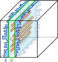
Figure 4: A component of $\bar{S}^{\prime}$ contained in a component of $\bar{S}$. Both contain the segments of simple geodesics in $S$.

The advantage of $\bar{S}^{\prime}$ over $\bar{S}$ is that it has a nicer decomposition into “wide enough” flow boxes (see Figure 4). We use the bound from Lemma 4.4 to get a bound on the measure:

$$\mu(\bar{S}^{\prime})\leq\mu(\bar{S})\leq\mu(B)\left(\epsilon+O(1/k)+O(k/g)+\left\{1-\frac{1}{O(1)}k\mu(B)\right\}^{\alpha k}\right).$$

Moreover, the connected components of $\bar{S}^{\prime}$ are all unions of the boxes $P_{\sigma}$. Thus, each connected component $P$ has width $e^{-t}\eta$ for $t\leq L-c\log g$ in the expanding direction, and full width in the other two. In other words,

$$\mu(P)\geq e^{-L+c\log g}\mu(B).$$

Dividing the upper bound for $\mu(\bar{S}^{\prime})$ by this gives the desired result. ∎

Combining the previous Claim with Lemma 4.11 allows us to count the number of connected components of $\mathring{\bar{S}}$:

Claim 4.16.

The number of connected components of $\mathring{\bar{S}}$ satisfies

$$\operatorname{\#comp}(\mathring{\bar{S}})\leq O(1)e^{L}\mu(B)\left(\epsilon+O(1/k)+O(k/g)+\left\{1-\frac{1}{O(1)}k\mu(B)\right\}^{\alpha k}\right),$$

where $k=\min(\frac{L}{c\log g},g^{2/3})$, and $c$ sufficiently large (depending on $\epsilon$).

Proof.

Recall that

$$\mathring{\bar{S}}=\bar{S}^{\prime}\cap g_{-L}B$$

By Claim 4.15, the number of components of $\bar{S}^{\prime}$ satisfies

$$\operatorname{\#comp}(\bar{S}^{\prime})\leq e^{L-c\log g}\left(\epsilon+O(1/k)+O(k/g)+\left\{1-\frac{1}{O(1)}k\mu(B)\right\}^{\alpha k}\right).$$ (32)

From the way $\bar{S}^{\prime}$ was defined, it is a union of subboxes that have width $e^{-L+c\log g}\eta$ in the expanding direction. Thus, each component $P$ of $\bar{S}^{\prime}$ has width $e^{-t}\eta$ in the expanding direction, for $t<L-c\log g$, and full width in the geodesic flow and contracting direction. Thus by Lemma 4.11

$$\operatorname{\#comp}(P\cap g_{-L}B)\leq O(1)e^{-t+L}\mu(B)$$

for each $P$. But $t<L-c\log g$, so we have

$$\operatorname{\#comp}(P\cap g_{-L}B)\leq O(1)e^{c\log g}\mu(B).$$ (33)

Taking the product of the bounds (32) and (33), we see that the number of components of $\mathring{\bar{S}}=\bar{S}^{\prime}\cap g_{-L}B$ satisfies the desired bound

∎

The proposition now follows by putting together Claim 4.14 and Claim 4.16.

∎

4.7 Completing the proof of 1.1

Proposition 4.17.

Fix $\delta,s_{0},\epsilon>0$. There exists a constant $d$ such that for any $\delta$-expander surface $X$ of genus $g$ with systole at least $s_{0}$, and $L>d\sqrt{g}\log g$,

$$N_{simp}(X,L)\leq\epsilon\cdot e^{L}/L.$$

Proof.

Fix $\epsilon>0$. Fix $\eta$ with $0<\eta<s_{0}$. For each $v\in T^{1}X$, let $B=B(v)$ be an $\eta$ flow box centered at $v$. For each $\eta$ much smaller than the systole of $X$, for all $v\in T^{1}X$, we have that $B(v)$ is embedded in $T^{1}X$.

Recall that $N_{simp}(B,L,\eta)$ is defined to be the number of geodesic segments of length $\eta$ in $B$ that lie on a simple closed geodesic of length $\ell$, with $L-\eta\leq\ell\leq L+\eta$. This number is related to the number of simple closed curves that pass through $B$, but if a simple closed curve passes through $B$ multiple times, then we count it multiple times. By 4.13, for any fixed $\epsilon^{\prime}>0$, there is a $c>0$ so that

$$N_{simp} (B,L,\eta)$$ (34)

$$\leq e^{L}\mu(B)\left(O(\epsilon^{\prime})+O(1/k)+O(k/g)+\left\{1-\frac{1}{O(1)}k\mu(B)\right\}^{\alpha k}\right)$$ (35)

for any $k<\frac{L}{c\log g}-1$.

Claim 4.18.

There exists $d$ (depending on $\epsilon$) such that if $L>d\sqrt{g}\log g$, then

$$N_{simp}(B,L,\eta)\leq\epsilon\cdot e^{L}\mu(B).$$

Proof.

For any choice of $d>c$, take

$$k=\min\left(\frac{L}{c\log g}-1,\frac{1}{d}g^{2/3}\right).$$

The reason for including $\frac{1}{d}g^{2/3}$ in the min is to ensure that the $O(k/g)$ error term in (35) is small.

Then $L>d\sqrt{g}\log g$ implies

$$\frac{d}{c}\sqrt{g}<k.$$

Using this, we can estimate the terms in the second factor of (35).

First, we can choose $\epsilon^{\prime}$ so that the $O(\epsilon^{\prime})$ term is bounded above by $\epsilon/3$. Note that this gives us a fixed choice of $c$ that we will use for the remainder of the proof.

Next, we have that

$$O(1/k)+O(k/g)=O\left(\frac{c}{d\sqrt{g}}\right)+O\left(\frac{1}{dg^{1/3}}\right)=\frac{1}{d}O(g^{-1/3}).$$

So we can choose $d$ large enough so that for all $g$, the $O(1/k)+O(k/g)$ term is also bounded above by $\epsilon/3$.

Now we use the estimate

$$\left\{1-\frac{1}{O(1)}k\mu(B)\right\}^{\alpha k} \leq e^{-\frac{\alpha}{O(1)}\mu(B)k^{2}}.$$

(This approximation can be justified with the inequality $1-x\leq e^{-x}$ for $x\geq 0$, since $\frac{1}{O(1)}k\mu(B)<1$ if $d$ is chosen appropriately, using that $\mu(B)=O(1/g)$ and $k\leq\frac{1}{d}g^{2/3}$. Recall that $\{x\}:=\max(x,0)$.)

Since $k>\frac{d}{c}\sqrt{g}$, and $\mu(B)=O(1/g)$, we have

$$-\frac{\alpha}{O(1)}\mu(B)k^{2}=-dO(1).$$

So we again increase $d$ if needed so that

$$\left\{1-\frac{1}{O(1)}k\mu(B)\right\}^{\alpha k}\leq e^{-dO(1)}<\epsilon/3.$$

We have now appropriately bounded all the error terms in (35), so we conclude the Claim. ∎

Now instead of just focusing on a single flow box $B$, we let $N_{simp}(X,[L-\eta,L+\eta])$ be the number of simple closed geodesics on all of $X$, which have length $\ell$, for $L-\eta\leq\ell\leq L+\eta$. We estimate $N_{simp}(X,[L-\eta,L+\eta])$ by integrating $N(B(v),L,\eta)$ over flow boxes centered over vectors $v\in T^{1}X$. By the same argument as in the proof of Theorem 3.1,

$$N_{simp}(X,[L-\eta,L+\eta])\leq(1+o(1))\frac{\eta}{L-\eta}\frac{1}{\mu(B)}\int_{T^{1}X}N_{simp}(B(w),L,\eta)d\mu_{w}$$

where for each $w\in T^{1}X$, $B(w)$ is the $\eta$ flow box centered at $w$.

For all $L$ large enough, $\frac{1}{L-\eta}<\frac{1+\epsilon}{L}$. As $L>d\sqrt{g}\log g$, we can again increase $d$ if necessary so that this is the case for all $g$. By 4.18, $N_{simp}(B(w),L,\eta)<\epsilon\cdot\mu(B)e^{L}$, so we get

$$N_{simp}(X,[L-\eta,L+\eta]) \leq\epsilon(1+\epsilon)\cdot\eta\frac{e^{L}}{L}.$$

for all $L>d\sqrt{g}\log g$.

Recall that $N_{simp}(X,L)$ is the total number of simple closed geodesics of length at most $L$. Then, trivially,

$$N_{simp}(X,L)\leq N(X,L/2)+N_{simp}(X,[L/2,L])$$

where $N_{simp}(X,[L/2,L])$ is the number of simple closed geodesics of length in $[L/2,L]$. By Theorem 3.1, for $\epsilon^{\prime}$ as in equation (35),

$$N(X,L/2)\leq(1+\epsilon^{\prime})\frac{e^{L/2}}{L}$$

since our lower bound on $L$ implies $L>c\log g$. Thus, since $L>d\sqrt{g}\log g$, we have that for $d>c$ large enough

$$N(X,L/2)<\epsilon\cdot\frac{e^{L}}{L}.$$

So, if we bound $N_{simp}(X,[L/2,L])$, then we are done. We write:

$$N_{simp}(X,[L/2,L])\leq\sum_{i=L/{2\eta}}^{L/\eta}N_{simp}(X,[\eta(i-1),\eta(i+1)]).$$

Doubling $d$ if we have to, we use that since $L/2>\frac{d}{2}\sqrt{g}\log g$, then for all $i$ with $\eta i\geq L/2$,

$$N_{simp}(X,[\eta(i-1),\eta(i+1)]) <\epsilon(1+\epsilon)\cdot\eta\frac{e^{i\eta}}{i\eta}$$

$$\leq\epsilon(1+\epsilon)\cdot\eta\frac{e^{i\eta}}{L/2}.$$

Next,

$$\sum_{i=L/2\eta}^{L/\eta}e^{i\eta} =\frac{e^{L+\eta}-e^{L/2}}{e^{\eta}-1}\leq\frac{e^{\eta}}{e^{\eta}-1}e^{L}.$$

Thus,

$$N_{simp}(X,[L/2,L])\leq 2\epsilon(1+\epsilon)\cdot\frac{\eta e^{\eta}}{e^{\eta}-1}\frac{e^{L}}{L}.$$

In other words, for any $\epsilon>0$, we can find a $d>c>0$ so that $L>d\sqrt{g}\log g$ implies

$$N_{simp}(X,L)\leq\frac{e^{L}}{L}\left(\epsilon+2\epsilon(1+\epsilon)\cdot\frac{\eta e^{\eta}}{e^{\eta}-1}\right).$$

Since $\eta$ is fixed, the term $\frac{\eta e^{\eta}}{e^{\eta}-1}$ is just some constant, and we have proved the desired result.

∎

Proof of 1.1.

We combine 4.17 and 3.1. ∎

5 Filling geodesics

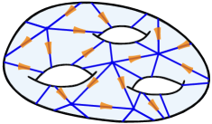
Figure 5: The projection of any closed geodesic that intersects all the orange flow boxes (which are actually in the unit tangent bundle $T^{1}X$) has a subset homeomorphic to the blue triangulation, and is hence filling. The blue triangulation is obtained by finding a “net” of points that are neither too close together, nor too separated, and then taking the associated Delaunay triangulation. The resulting triangles have bounded geometry, which means that the orange flow boxes can be taken to be uniformly sized.

In this section we prove 1.4. Throughout, $X$ is a $\delta$-expander surface with $\operatorname{systole}(X)>s_{0}$.

5.1 Flow boxes to detect filling geodesics

Lemma 5.1.

There exists $\eta>0$ and $C$ (depending only on the systole bound $s_{0}$), and $\eta$ flow boxes $B_{1},\ldots,B_{Cg}\subset T^{1}X$ such that if $\gamma$ is a closed geodesic that intersects every $B_{i}$, then $\gamma$ is filling.

Proof.

The idea of the proof is illustrated in Figure 5. Choose a finite collection of discs $D_{i}$ of radius $r\leq s_{0}/6$ that cover $X$ (we may need to make $r$ smaller than this, as discussed later in the proof). By the $3$-times covering lemma, among these discs, we can find $D_{1},\ldots,D_{k}$ that are disjoint, and such that $3D_{1},\ldots,3D_{k}$ (where $3D_{i}$ is the disc with the same center as $D_{i}$, and $3$ times the radius) cover $X$. Let $p_{i}$ be the center of $D_{i}$.

Now let $\mathcal{D}$ be the Delaunay triangulation of $X$ with respect to the set of vertices $\{p_{1},\ldots,p_{k}\}$ (it is possible to get a Delaunay tessellation where some of the faces are not triangles; if so we perturb the points very slightly, and then we will get a triangulation).

Figure 6: The edge length bounds and Delaunay property give control of angles

Claim 5.2.

For any triangle in $\mathcal{D}$, the edge lengths lie in $[2r,6r]$ and angles at most $150^{\circ}$.

Proof.

For the lower bound on edge lengths, note that since the discs $D_{1},\ldots,D_{k}$ are disjoint, any pair of distinct centers cannot be closer than distance $2r$.

For the upper bound on edge lengths, first note that any point in $X$ is at most distance $3r$ from one of $p_{1},\ldots,p_{k}$, since the discs $3D_{1},\ldots,3D_{k}$ are assumed to cover $X$. This implies that in the Voronoi tessellation with respect to $\{p_{1},\ldots,p_{k}\}$, any point $x$ in the Voronoi cell $V_{i}$ containing $p_{i}$ satisfies $d(x,p_{i})\leq 3r$. So if $V_{i},V_{j}$ are adjacent Voronoi cells, then $d(p_{i},p_{j})\leq 6r$. Since the Delaunay triangulation is the dual of the Voronoi tessellation, all edges in $\mathcal{D}$ must have length at most $6r$.

To prove the claim about angles, we first note that, using the properties just proved, any triangle in $\mathcal{D}$ lies in a ball of radius $6r$, which we can assume is sufficiently small so that the geometry in this ball is very close to Euclidean (we can define $r$ smaller if necessary; this would be a problem if it depended on the surface/genus, but it does not need to here). In Euclidean space, the Delaunay triangulation has the property that the disc bounded by any circumcircle of one of its triangles does not contain any other Delaunay vertex. Since every point of $X$ has distance at most $3r$ to the vertex set of $\mathcal{D}$, we then see that the radius of this circumcircle is at most $3r$.

The desired lower bound on angles then will follow from this Euclidean geometry fact (see Figure 6): if $ABC$ is a triangle whose circumcircle is centered at $P$ and such that the line $BC$ separates $A$ from $P$, then

$$\angle BAC=180^{\circ}-2\arcsin\left(\frac{|BC|}{2\cdot|PB|}\right).$$

For $ABC$ one of our Delaunay triangles, we have $|BC|\geq 2r$, and $|PB|\leq 3r$. Using these in the above gives $\angle BAC\leq 180^{\circ}-2\arcsin(1/3)\leq 150^{\circ}$.

∎

Now we will define the flow boxes $B_{1},\ldots,B_{k}$. For each edge $e_{i}$ of $\mathcal{D}$, let $v_{i}$ be one of the two vectors tangent to $e_{i}$ at its midpoint. Then we let $B_{i}:=B(v_{i})$ be the $\eta$ flow box centered at $v_{i}$. If we take $\eta$ sufficiently small, then any closed geodesic $\gamma$ that intersects all such $B_{i}$ will contain a subset whose projection to the surface is a graph that differs from $\mathcal{D}$ by a small homeomorphism. In particular, since $\mathcal{D}$ fills the surface (every component of its complement is a topological disc, since it’s just a triangle), $\gamma$ will also be filling. Because of the upper bound on edge lengths of $\mathcal{D}$, and upper bound on angles (which implies a lower bound on angles, since all the triangles are small, hence close to Euclidean), we can take $\eta$ to be uniform (depending only on systole lower bound $s_{0}$, and not on other features of the surface such as the genus).

Figure 7: The Delaunay vertices have bounded degree

All that remains is to estimate $k$, the number of the $B_{i}$. First, note that $\operatorname{\#vertices}(\mathcal{D})\leq c\cdot g$, for some $c$ depending only on the systole lower bound $s_{0}$. This is because the discs $D_{1},\ldots,D_{k}$, whose centers are exactly the vertices of $\mathcal{D}$, are disjoint and have radius $r$ (depending only on systole bound $s_{0}$), while the area of the surface $X$ is $(4g-4)\pi$. The valence of each vertex $p_{i}$ in $\mathcal{D}$ is uniformly bounded by some $d$. In fact, for each vertex $p_{j}$ that is a neighbor of $p_{i}$, the disc $D_{i}$ centered at $p_{i}$ is entirely contained in the ball of radius $7r$ about $p$; since each such $D_{i}$ has radius $r$ and they are disjoint, there is a bounded number of them. See Figure 7. Hence

$$\operatorname{\#edges}(\mathcal{D})\leq d\cdot\operatorname{\#vertices}(\mathcal{D})\leq d\cdot c\cdot g.$$

Since $k=\operatorname{\#edges}(\mathcal{D})$, taking $C=dc$ gives the desired bound of $Cg$ flow boxes.

∎

5.2 Geodesics avoiding flow boxes

Lemma 5.3.

Fix $\epsilon>0$ and $C>0$. There exists a constant $c$ with the following property. Let $\mathcal{B}=\{B_{1},\ldots,B_{Cg}\}$ be any collection of $\eta$ flow boxes in $T^{1}X$. Let

$$N_{\mathcal{B}}(X,L):=\#\{\gamma\text{ closed geodesic on }X:\ell(\gamma)\leq L,\ \exists B\in\mathcal{B}\text{ s.t. }\gamma\cap B=\emptyset\},$$

i.e. the number of closed geodesics that avoid some element of $\mathcal{B}$. Then for any $L>cg(\log g)^{2}$,

$$N_{\mathcal{B}}(X,L)\leq\epsilon\cdot e^{L}/L.$$

Proof.

We will first study the geodesics starting in some particular flow box. So fix $B$ an $\eta/3$ flow box. Then let $N_{\mathcal{B}}(B,L,\eta/3)$ denote the number of geodesic segments of length $\eta/3$ in $B$ that are part of a closed geodesic of length in $[L-\eta/3,L+\eta/3]$ that does not intersect some element of $\mathcal{B}$. Our first goal is to upper bound $N_{\mathcal{B}}(B,L,\eta/3)$, and then we will use this to upper bound $N_{\mathcal{B}}(X,L)$.

Claim 5.4.

We have

$$N_{\mathcal{B}}(B,L,\eta/3)\leq\epsilon\cdot\mu(B)e^{L}.$$

We will prove this after 5.5 below. In preparation, we will study measures of sets of tangent vectors in $B$ that avoid some element of $\mathcal{B}$, without the condition of being tangent to an actual closed geodesic.

Let $\mathcal{B}^{-}:=\{B_{1}^{-},\ldots,B_{Cg}^{-}\}$ be contracted flow boxes. Let

$$t_{1}=c^{\prime}\log g,\ t_{2}=2c^{\prime}\log g,\ \ldots,\ t_{k}=kc^{\prime}\log g,\ t_{k+1}=L,$$

where $c^{\prime}$ and $k$ will also be chosen later. Then let

$$S_{\mathcal{B}^{-}}:=\{v\in B\cap g_{-L}B:\{g_{t}v\}_{t=0}^{L}\cap B_{i}^{-}=\emptyset\text{ for some }i=1,\ldots,Cg\},$$

i.e. the set of those tangent vectors that avoid some element of $\mathcal{B}^{-}$. We will bound the measure of $S_{\mathcal{B}^{-}}$ from above. Let $k=\lceil dg\log g\rceil$, where $d$ is a constant that will be specified later. We want the gap between every successive pair to be at least $c^{\prime}\log g$, for $c^{\prime}$ the constant in Lemma 5.8, which we will apply shortly. To ensure this, we need

$$L>(k+1)c^{\prime}\log g=(dg\log g+1)c^{\prime}\log g.$$

Since the right-hand term is $O(g(\log g)^{2})$, the above inequality will hold if we take the $c$ in the current lemma sufficiently large.

Now with these $t_{i}$, we have

$$S_{\mathcal{B}^{-}}\subset\{v\in B\cap g_{-L}B:\{g_{t_{1}}v,\ldots,g_{t_{k}}v\}\cap B_{i}^{-}=\emptyset\text{ for some }i=1,\ldots,Cg\}.$$

To bound the measure of the right-hand side above, we use Lemma 5.8 (which gives us the value of $c^{\prime}$) with flow boxes $B,B_{1},\ldots,B_{Cg}$, giving

$$\mu(S_{\mathcal{B}^{-}}) \leq(1+\epsilon)\mu(B)^{2}\sum_{i=1}^{Cg}\left[1-(1-\epsilon)\mu(B_{i})\right]^{k}$$ (36)

$$=(1+\epsilon)\mu(B)^{2}(Cg)\left[1-(1-\epsilon)\mu(B_{i})\right]^{k}$$ (37)

$$\leq(1+\epsilon)\mu(B)^{2}(Cg)\left[1-\frac{1}{O(1)g}\right]^{k}.$$ (38)

Now we use the approximation

$$g\left(1-\frac{1}{O(1)g}\right)^{k}\leq O(1)g\exp\left(-\frac{1}{O(1)g}\right)^{k}\leq O(1)g\exp\left(\frac{-k}{O(1)g}\right),$$

which can be made arbitrarily small by choosing $d$ large, since $k\geq dg\log g$. Applying this to (38) we get

$$\mu(S_{\mathcal{B}^{-}})\leq\epsilon\cdot\mu(B)^{2}.$$ (39)

Claim 5.5.

At most $\kappa:=4\sqrt{\epsilon}$ fraction of the components of $B\cap g_{-L}B$ are completely contained in $S_{\mathcal{B}^{-}}$.

Proof.

Assume the contrary. Let $N=\operatorname{\#comp}(B\cap g_{-L}B)$, and let $P_{1},\ldots,P_{N}$ be the components of $B\cap g_{-L}B$, ordered such that $\mu(P_{1})\leq\cdots\leq\mu(P_{N}).$ Then

$$\mu(S_{\mathcal{B}^{-}})\geq\sum_{i<\kappa N}\mu(P_{i})\geq\sum_{(\kappa/2)N<i<\kappa N}\mu(P_{i})\geq\mu(P_{\lfloor(\kappa/2)N\rfloor})\cdot(\kappa/2)N.$$

Using that $N\geq\mu(B)e^{L}$, which follows from effective mixing and the contraction/expansion (as in proof of 3.1), and (39), we get that

$$\mu(P_{\lfloor(\kappa/2)N\rfloor})\leq\mu(S_{\mathcal{B}^{-}})\cdot\frac{2}{\kappa\cdot N}\leq\epsilon\cdot\mu(B)^{2}\frac{2}{4\sqrt{\epsilon}\mu(B)e^{L}}=\frac{\sqrt{\epsilon}}{2}\cdot e^{-L}\mu(B).$$

On the other hand, by effective mixing, 2.2, applied to smaller flow boxes, we see that the components of $B\cap g_{-L}B$ have widths in the flow direction that are close to equidistributed in $[0,\eta/3]$. Combined with our understanding of the shape of these components in the contracting and expanding directions, we get

$$\mu(P_{\lfloor(\kappa/2)N\rfloor})\geq\frac{1}{2}\cdot(\kappa/2)e^{-L}\mu(B)=\frac{1}{2}(2\sqrt{\epsilon})e^{-L}\mu(B)=\sqrt{\epsilon}\cdot e^{-L}\mu(B),$$

contradicting the inequality above.

∎

Proof of 5.4.

Observe that if $v\in B\cap g_{-L}B$ and $v\not\in S_{\mathcal{B}^{-}}$, then for any $w$ in $v$’s connected component of $B\cap g_{-L}B$, we have $w\not\in S_{\mathcal{B}}$. This is because all vectors in the component travel closely together up to time $L$, and since $\{g_{t}v\}$ hits every $B_{i}^{-}$, we see that $\{g_{t}w\}$ will hit every $B_{i}$.

Thus any segment counted by $N_{\mathcal{B}}(B,L,\eta/3)$ intersects a component of $B\cap g_{-L}B$ that is entirely contained in $S_{\mathcal{B}^{-}}$; let $K$ be the number of such components. It follows from 5.5 that

$$K\leq 4\sqrt{\epsilon}\cdot\operatorname{\#comp}(B\cap g_{-L}B)\leq 4\sqrt{\epsilon}\cdot\mu(B)e^{L}.$$

Now Lemma 6.2 implies that each component of $B\cap g_{-L}B$ intersects at most one $\eta/3$ segment of a closed geodesic with length in $[L-\eta/3,L+\eta/3]$. So

$$N_{\mathcal{B}}(B,L,\eta/3) \leq K$$

$$\leq 4\sqrt{\epsilon}\cdot\mu(B)e^{L}.$$

Choosing $\epsilon$ appropriately gives the desired result.

∎

To complete the proof of the lemma, we upper bound $N_{\mathcal{B}}(X,L)$ using 5.4, an upper bound on $N_{\mathcal{B}}(B,L,\eta/3)$. The first step is to follow the analogous part of proof of 3.1, which involves averaging over all possible start boxes $B$, to get

$$N_{\mathcal{B}}(X,[L-\eta/3,L+\eta/3])\leq\epsilon\cdot(\eta/3)\cdot\frac{e^{L}}{L},$$

where the left-hand side denotes the number of closed geodesics of length in $[L-\eta/3,L+\eta/3]$ for which there is some element of $\mathcal{B}$ that the geodesic does not intersect. By enlarging $d$ if necessary, we get the above bound with $L$ replaced by any value between $L/2$ and $L$. We then sum over these values, as in the end of the proof of 4.17.

∎

Remark 5.6.

In 5.5 above, we used equidistribution of widths of intersection components in the flow direction. This technique was not used in proof of 1.1. An alternate way to prove that theorem would be the control the shape of components throughout the proof, and then get a measure bound on the relevant subset of $B\cap g_{-L}B$. The desired bound on number of simple closed geodesics could then be deduced from the measure bound using the equidistribution as above.

On the other hand, there is another way of proving Lemma 5.3 avoiding the use of the equidistribution result. This involves some more steps, as in proof of 1.1, to account for non-fullness of intersection components in the geodesic flow direction. ∎

Lemma 5.8 below was used in the proof of Lemma 5.3 above; Lemma 5.7 is used in the proof of Lemma 5.8.

Lemma 5.7.

Fix $\delta,\epsilon>0$. There exists some $c>0$ such that for any $\delta$-expander surface $X$ the following holds. Let $B_{0},\ldots,B_{k}\subset T^{1}X$ be $\eta$ flow boxes. For each $i$, let $E_{i}$ be either $B_{i}$, or the complement in $T^{1}X$ of $B_{i}$, and let

$$m_{i}=\left\{\begin{array}[]{lll}(1+\epsilon)\mu(B_{i})&\text{ if }&E_{i}=B_{i}\\ 1-(1-\epsilon)\mu(B_{i})&\text{ if }&E_{i}=T^{1}X-B_{i}.\end{array}\right.$$

Then

$$\mu\left(\{v:g_{t_{i}}v\in E_{i}\text{, for }i=0,\ldots,k\}\right)\leq m_{0}\cdots m_{k}$$

for any $t_{0}<\cdots<t_{k}$ with $t_{i}-t_{i-1}\geq c\log g$ for each $i\geq 1$.

Proof.

The proof is similar to that of 2.2. To ensure the complementary components are thick enough, we use slightly contracted flow boxes.

∎

Next we get an upper bound on the measure of those $v$ avoiding some box $B_{1},\ldots,B_{m}$ at all the prescribed times.

Lemma 5.8.

Fix $\epsilon>0$. There exists a constant $c$ with the following property. Let $B,B_{1},\ldots,B_{m}\subset T^{1}X$ each either an $\eta$ or $\eta/3$ flow box. Then

$$\mu\left(\{v\in B\cap g_{-t_{k+1}}B:\{g_{t_{1}}v,\ldots,g_{t_{k}}v\}\cap B_{i}=\emptyset\text{ for some }i=1,\ldots,m\}\right)$$

$$\leq(1+\epsilon)\mu(B)^{2}\sum_{i=1}^{m}\left[1-(1-\epsilon)\mu(B_{i})\right]^{k}$$

for any $t_{1}<\cdots<t_{k+1}$ with $t_{i}-t_{i-1}\geq c\log g$ for each $i\geq 2$.

Proof.

For $i=1,\ldots,m$, let

$$S_{i}=\{v\in B\cap g_{-t_{k+1}}B:\{g_{t_{1}}v,\ldots,g_{t_{k}}v\}\cap B_{i}=\emptyset\}.$$

We have

$$\mu\left(S_{i}\right) =\mu\left(\{v\in B\cap g_{-t_{k+1}}B:g_{t_{1}}v,\ldots,g_{t_{k}}v\in T^{1}X-B_{i}\}\right)$$ (40)

$$\leq(1+\epsilon)^{2}\mu(B)^{2}\cdot\left[1-(1-\epsilon)\mu(B_{i})\right]^{k},$$ (41)

by Lemma 5.7.

Then by a union bound

$$\mu\big{(}\{v\in B\cap g_{-t_{k+1}}B :\{g_{t_{1}}v,\ldots,g_{t_{k}}v\}\cap B_{i}=\emptyset\text{ for some }i=1,\ldots,m\}\big{)}$$

$$=\mu\left(\bigcup_{i=1}^{m}S_{i}\right)$$

$$\leq\sum_{i=1}^{m}\mu(S_{i})$$

$$\leq\sum_{i=1}^{m}(1+\epsilon)^{2}\mu(B)^{2}\cdot\left[1-(1-\epsilon)\mu(B_{i})\right]^{k},$$

where in the last line we have used (41).

∎

5.3 Completing proof of 1.4

Proof of 1.4.

Let $\mathcal{B}:=\{B_{1},\ldots,B_{Cg}\}$ be flow boxes given by Lemma 5.1. By that lemma, we have $N(X,L)-N_{fill}(X,L)\leq N_{\mathcal{B}}(X,L)$. We combine this with Lemma 5.3 applied with these flow boxes, to get

$$N(X,L)-N_{fill}(X,L)\leq N_{\mathcal{B}}(X,L)\leq\epsilon\cdot e^{L}/L.$$

We then compare this to the estimate of the number of all closed geodesics $N(X,L)$ given by 3.1 to conclude the desired result. ∎

6 Appendix: Anosov Closing Lemma

We use the following two lemmas relating components of $B\cap g_{-L}B$ to closed geodesics of length approximately $L$ passing through $B$.

Lemma 6.1.

For any $\eta$ sufficiently small (depending on systole bound $s_{0}$) the following holds. Let $B\subset T^{1}X$ be an embedded $\eta$ flow box. For any $L$ let $N(B,L,\eta)$ be the number of length $\eta$ geodesics segments inside of $B$ that lie on a closed geodesic of length in $[L-\eta,L+\eta]$. Then

$$\left|N(B,L,\eta)-\operatorname{\#comp}(B\cap g_{-L}B)\right|=O(1).$$

Proof.

This is a version of the Anosov Closing Lemma. See, for instance, [KH95, Lemma 20.6.5]. ∎

We also need the following result, which is similar to part of the bound above, but counts any closed geodesic intersecting $B$, even if does not intersect for the full time $\eta$ (which can happen because our flow boxes do not behave exactly like Euclidean rectangular boxes).

Lemma 6.2.

For any $\eta$ sufficiently small (depending on systole bound $s_{0}$) the following holds. Let $B\subset T^{1}X$ be an embedded $\eta$ flow box. Suppose that $\gamma_{1},\gamma_{2}$ are closed geodesics with period in $[L-\eta,L+\eta]$. For any $L$, if $v_{1},v_{2}$ are in the same component of $B\cap g_{-L}B$ and $v_{i}$ is tangent to $\gamma_{i}$ for $i=1,2$, then $\gamma_{1}=\gamma_{2}$.

Proof.

The components of $B\cap g_{-L}B$ have width at most $e^{-L}\eta$ in the expanding direction. Since $v_{1},v_{2}$ are in the same component, for each $t\in[0,L]$ there exists some embedded $\eta$ flow box that contains $g_{t}v_{1}$ and $g_{t}v_{2}$. It follows that $\gamma_{1},\gamma_{2}$ are homotopic. Since $X$ is hyperbolic, they must be the same. ∎

References

- [AM23] Nalini Anantharaman and Laura Monk, Friedman-Ramanujan functions in random hyperbolic geometry and application to spectral gaps, arXiv e-prints (2023), arXiv:2304.02678.
- [BK89] Andrei Z. Broder and Anna R. Karlin, Bounds on the cover time, J. Theoret. Probab. 2 (1989), no. 1, 101–120. MR 981768
- [BM04] Robert Brooks and Eran Makover, Random construction of Riemann surfaces, J. Differential Geom. 68 (2004), no. 1, 121–157. MR 2152911
- [Bus78] Peter Buser, Cubic graphs and the first eigenvalue of a Riemann surface, Math. Z. 162 (1978), no. 1, 87–99. MR 505920
- [Bus10] , Geometry and spectra of compact Riemann surfaces, Modern Birkhäuser Classics, Birkhäuser Boston, Ltd., Boston, MA, 2010, Reprint of the 1992 edition. MR 2742784
- [CF05] Colin Cooper and Alan Frieze, The cover time of random regular graphs, SIAM J. Discrete Math. 18 (2005), no. 4, 728–740. MR 2157821
- [DS22] Benjamin Dozier and Jenya Sapir, Simple vs non-simple loops on random regular graphs, arXiv e-prints (2022), arXiv:2209.11218.
- [Gam06] Alex Gamburd, Poisson-Dirichlet distribution for random Belyi surfaces, Ann. Probab. 34 (2006), no. 5, 1827–1848. MR 2271484
- [GPY11] Larry Guth, Hugo Parlier, and Robert Young, Pants decompositions of random surfaces, Geom. Funct. Anal. 21 (2011), no. 5, 1069–1090. MR 2846383
- [HM21] Will Hide and Michael Magee, Near optimal spectral gaps for hyperbolic surfaces, arXiv e-prints (2021), arXiv:2107.05292.
- [KH95] Anatole Katok and Boris Hasselblatt, Introduction to the modern theory of dynamical systems, Encyclopedia of Mathematics and its Applications, vol. 54, Cambridge University Press, Cambridge, 1995, With a supplementary chapter by Katok and Leonardo Mendoza. MR 1326374
- [LW21] Michael Lipnowski and Alex Wright, Towards optimal spectral gaps in large genus, arXiv e-prints (2021), arXiv:2103.07496.
- [Mar04] Grigoriy A. Margulis, On some aspects of the theory of Anosov systems, Springer Monographs in Mathematics, Springer-Verlag, Berlin, 2004, With a survey by Richard Sharp: Periodic orbits of hyperbolic flows, Translated from the Russian by Valentina Vladimirovna Szulikowska. MR 2035655
- [Mat13] Carlos Matheus, Some quantitative versions of Ratner’s mixing estimates, Bull. Braz. Math. Soc. (N.S.) 44 (2013), no. 3, 469–488. MR 3124746
- [Mir08] Maryam Mirzakhani, Growth of the number of simple closed geodesics on hyperbolic surfaces, Ann. of Math. (2) 168 (2008), no. 1, 97–125. MR 2415399
- [Mir13] , Growth of Weil-Petersson volumes and random hyperbolic surfaces of large genus, J. Differential Geom. 94 (2013), no. 2, 267–300. MR 3080483
- [MNP22] Michael Magee, Frédéric Naud, and Doron Puder, A random cover of a compact hyperbolic surface has relative spectral gap , Geom. Funct. Anal. 32 (2022), no. 3, 595–661. MR 4431124
- [MP19] Maryam Mirzakhani and Bram Petri, Lengths of closed geodesics on random surfaces of large genus, Comment. Math. Helv. 94 (2019), no. 4, 869–889. MR 4046008
- [MT22] Laura Monk and Joe Thomas, The tangle-free hypothesis on random hyperbolic surfaces, Int. Math. Res. Not. IMRN (2022), no. 22, 18154–18185. MR 4514465
- [NWX23] Xin Nie, Yunhui Wu, and Yuhao Xue, Large genus asymptotics for lengths of separating closed geodesics on random surfaces, J. Topol. 16 (2023), no. 1, 106–175. MR 4532491
- [Rat87] Marina Ratner, The rate of mixing for geodesic and horocycle flows, Ergodic Theory Dynam. Systems 7 (1987), no. 2, 267–288. MR 896798
- [Riv01] Igor Rivin, Simple curves on surfaces, Geom. Dedicata 87 (2001), no. 1-3, 345–360. MR 1866856
- [WX21] Yunhui Wu and Yuhao Xue, Random hyperbolic surfaces of large genus have first eigenvalues greater than , arXiv e-prints (2021), arXiv:2102.05581.
- [WX22] , Prime geodesic theorem and closed geodesics for large genus, arXiv e-prints (2022), arXiv:2209.10415.