An Artificial Neural Network-based Density Functional Approach for Adiabatic Energy Differences in Transition Metal Complexes

Abstract

During the past decades, approximate Kohn-Sham density-functional theory schemes garnered many successes in computational chemistry and physics; yet the performance in the prediction of spin state energetics is often unsatisfactory. By means of a machine-learning approach, an enhanced exchange and correlation functional is developed to describe adiabatic energy differences in transition metal complexes. The functional is based on the computationally efficient revision of the regularized strongly constrained and appropriately normed (R2SCAN) functional and improved by an artificial neural-network-correction trained over a small dataset of electronic densities, atomization energies and/or spin state energetics. The training process, performed using a bio-inspired non gradient-based approach adapted for this work from Particle Swarm Optimization, is discussed in detail. The meta-GGA functional is finally shown to outperform most known density functionals in the prediction of adiabatic energy differences for both the validation test and the generality test.

SIMaP] Université Grenoble Alpes, CNRS, Grenoble INP, SIMaP, 38000 Grenoble, France SIMaP] Université Grenoble Alpes, CNRS, Grenoble INP, SIMaP, 38000 Grenoble, France LIG] Université Grenoble Alpes, CNRS, Grenoble INP, LIG, 38000 Grenoble, France SIMaP] Université Grenoble Alpes, CNRS, Grenoble INP, SIMaP, 38000 Grenoble, France SIMaP] Université Grenoble Alpes, CNRS, Grenoble INP, SIMaP, 38000 Grenoble, France

1 Introduction

Applied density-functional theory (DFT) has revolutionized the field of materials science by providing a powerful tool for predicting the electronic and structural properties of materials, enabling their design and discovery for a wide range of applications¹. Despite its many successes, DFT still faces several challenges that limit its predictive power and applicability ^{2, 3}. As an example, one can metion the calculation of spin-state energetics in transition metal complexes^{4, 5, 6, 7, 8, 9}. This has strong implications in the assistance and guidance alongside experimental efforts towards, for example, the design of novel spin crossover (SCO) complexes. The vast majority of SCO materials, which are of great interest for applications such as molecular spintronics, molecular electronics, and sensors^{10, 11, 12, 13} are octahedrally coordinated molecular complexes. For these complexes, the thermodynamics of the spin transition (i.e., the transition temperature T_1/2) between the low-spin (LS) and high-spin (HS) states is related to the adiabatic energy difference, $\Delta E$_H-L=$E$_HS-$E$_LS, i.e., the energy difference between the two spin states computed at their corresponding geometry.

The computational chemistry community has devoted a substantial effort in understanding the performance of approximate Khon-Sham density-functional theory (KS-DFT) schemes ^{14, 15, 7, 16, 17}. Large deviations in the values of the spin splitting energies are found among different families of exchange and correlation functionals. Semilocal functionals, such as the generalized gradient approximation (GGA), for example, tend to overstabilize LS, ^{14, 18, 19, 20, 21, 22} while Hartree–Fock (HF) overstabilizes HS ²³. In this context, hybrid functionals may be viewed as a possibility to alleviate the problem ^{23, 24, 17}. DFT+U was also studied in this respect^{25, 26, 27, 28, 29}. Recently, it was shown that the Hubbard $U$ correction in DFT+U may yield large errors in the spin-state energy difference of octahedral Fe-II complexes owing to the bias toward high-spin states imposed by the Hubbard term in the total energy³⁰. Later, a non-self consistent density-corrected scheme adopting the Hubbard $U$ density was shown to yield a good description of adiabatic energy differences for Fe(II)-based complexes³¹.

Recently, several studies have shown how density functional theory can benefit from machine learning (ML) techniques ^{32, 33, 34, 35, 36, 37, 38, 39, 40, 41, 42, 43}. Pioneer works like the one from Snyder et al. proved that is possible to learn the kinetic energy of 1D fermionic systems⁴³. Brockherde et al. developed a ML scheme to learn the density via the external potential/density Hohenberg–Kohn map, so that self consistency can be bypassed ⁴¹. Learning the exchange and correlation functional itself, as demonstrated by the pioneer work by Nagai et al.³⁷, has also been studied ^{37, 38, 33, 36, 34, 32}. In this class of methods, the exchange and correlation is replaced, adjusted, or corrected by an artificial neural network that receives as input functions of the electronic density.

These machine learning applications to KS-DFT use the supervised approach philosophy where the functional ”learns itself” from a given high quality set of data ^{44, 42}. An important aspect worth to be mentioned here is that the knowledge of the physical constraints that the exact exchange and correlation functional must fulfill can be exploited to create a strongly transferable functional. In this spirit, Nagai, Akashi, and Sugino ³² trained their ANN on the atomization energies and densities from single point calculations of three molecules, and showed that their resulting metal-GGA functional performed well in describing atomization energies of molecules not seen in the training, and also on computing equilibrium lattice constants for solids.

The aim of the present work is to extend upon the latter approach and train an exchange and correlation functional for a good description of electronic densities and adiabatic energy differences of transition metal complexes, as well as atomization energies and densities of simpler molecules. An important novelty of this work, is that the training process is explicitly shown and discussed in detail, thus allowing the reader to understand the optimization process and its limitations. The ML functional is trained using a bio-inspired non gradient-based approach adapted from Particle Swarm Optimization (PSO)⁴⁵. This class of optimization algorithms has shown success in handling intricate nonlinear loss functions⁴⁶ owing to the collective intelligence ingredient that improves the efficiency of the optimization process. These results show that by training a correction over R2SCAN using three light molecules and three diatomic (metal-nonmetal) transition molecules, the prediction of adiabatic energy differences are improved compared to the state-of-the-art in approximate KS-DFT at no expenses for the performance on atomization energies. Furthermore, the analysis of the non-gradient based training shows that the $\Delta E_{H-L}$ term dominates the optimization and that the electronic density plays an auxiliary role by accelerating the convergence of the loss function. Compared to the known density functional approaches tested here for comparison, the exchange and correlation functional optimized in this work exhibits the best performance for both the validation and the generality test.

2 Methodology

2.1 Density Functional Theory and Neural Network Functionals

In the KS-DFT framework, the total energy, $E_{\textup{tot}}$, and the electronic density, $\rho(\textbf{r})$, can be computed by solving the KS equations for non-interacting fermions⁴⁷

$$\left(-\frac{\hbar}{2m}\nabla^{2}+v_{\textup{eff}}\right)\phi_{i}=\varepsilon_{i}\phi_{i}.$$ (1)

In Eq. 1, the effective potential reads

$$v_{\textup{eff}}(\textbf{r})=v_{\textup{ext}}(\textbf{r})+\int\frac{\rho(\textbf{r})}{|\textbf{r}-\textbf{r}^{\prime}|}d\textbf{r}^{\prime}+\frac{\delta E_{\textup{xc}}[\rho(\textbf{r})]}{\delta\rho(\textbf{r})},$$ (2)

where $\rho(\textbf{r})=\sum\phi_{i}\phi_{i}^{*}$, $v_{\textup{ext}}(\textbf{r})$ is an external potential and $E_{\textup{xc}}$ is the functional of exchange and correlation. The exact form of $E_{\textup{xc}}$ is unknown and therefore must be approximated. By solving the eigen-equation presented in Eq. 1, one obtains the eigenvalues, $\varepsilon_{i}$, and eigenfunctions, $\phi_{i}$, that correspond to the Kohn-Sham energies and orbitals. Because $\rho(\textbf{r})$ is needed to build $v_{\textup{eff}}$ and therefore compute $E_{\textup{tot}}$, the set of equations above is solved self-consistently, i.e., $\rho(\textbf{r})$ is recomputed at iterations until convergence on the total energy and charge density is achieved. The dependency of the effective potential $v_{\textup{eff}}$ on $\rho$ is at the core of the mean-field theory of KS-DFT since it should mimic the electronic correlation of the many electrons system by adopting a non-interacting single particle scheme.

After solving the KS equations, the total energy can be written as

$$\begin{split}E=&\sum\varepsilon_{i}-\frac{e^{2}}{2}\iint\frac{\rho(\textbf{r})\rho(\textbf{r}^{\prime})}{|\textbf{r}-\textbf{r}^{\prime}|}d\textbf{r}^{\prime}d\textbf{r}+E_{\textup{xc}}[\rho(\textbf{r})]\\ &-\int\frac{\delta E_{\textup{xc}}[\rho(\textbf{r})]}{\delta\rho(\textbf{r})}\rho(\textbf{r})d\textbf{r}.\end{split}$$ (3)

The functional of exchange and correlation can be written as

$$E_{\textup{xc}}=\int\varepsilon_{\textup{xc}}[\rho(\textbf{r})]\rho(\textbf{r})d\textbf{r},$$ (4)

where $\varepsilon_{\textup{xc}}$ is the exchange and correlation energy density. The idea developed in this work, summarized in Figure 1, is to obtain a $\varepsilon_{\textup{xc}}$ as a correction over R2SCAN functional,⁴⁸ such that

$$\varepsilon_{\textup{xc}}=F_{x}\varepsilon_{\textup{x}}^{\textup{R2SCAN}}+F_{\textup{c}}\varepsilon_{\textup{c}}^{\textup{R2SCAN}}.$$ (5)

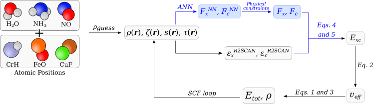
Figure 1: Schematic representation of a single point calculation performed in the present approach. The step where the ANN correction is explicitly applied over R2SCAN is highlighted in blue.

Recently, Nagai and co-workers³⁷ developed a new functional, defined as a correction over the strongly constrained and appropriately normed (SCAN)⁴⁹, trained on energies and densities of a small subset (three molecules only made up by first and second row elements) of the G2 dataset⁵⁰. The result showed an improvement over SCAN in the prediction of ionization potentials and atomization energies on the complete G2 dataset. Yet, previous reports on the literature pointed out some major numerical instabilities in some meta-GGA functionals ⁵¹ including SCAN itself, for electron densities rapidly changing in space. These manifest as sharp features of the energy derivatives and make the functional unstable over grid changes thus resulting in bad gradients estimation during the self-consistent field process ^{52, 53}. To solve this problem, Bartok and co-workers developed a regularized version of SCAN (rSCAN) which exhibit improved smoothness properties and improves SCAN’s numerical performance ⁵⁴. However, this improvement came at the expense of some of the physical limits originally obeyed by SCAN. R2SCAN⁴⁸ follows this implementation path, recovering most of the physical limits that SCAN originally had. The $17$ exact conditions applicable to meta-GGA (listed in the SI from Sun et al. ⁴⁹) were imposed in the original definition of SCAN and most of these conditions are present on R2SCAN. Only the fourth-order gradient expansion condition, lost in the rSCAN implementation, is not recovered.⁴⁸

In this work, in order to address the case of transition metal complexes, where rapid fluctuations of the electronic density are expected, a new ANN-based functional defined as a correction over R2SCAN is proposed. This choice allows us to circumvent the instabilities of SCAN that manifest themselves in large changes of the energy upon tiny changes of the density, as shown in Figure S1 for the FeO molecule. Such instability (observed for FeO and not for H₂O) is found when training a correction over SCAN. Finally, we impose that $\varepsilon_{\textup{xc}}$, defined in eq. 5, satisfies the physical limits imposed in R2SCAN using Lagrange multipliers, as done by Nagai and co-workers in their more recent work.³²

Figure 2 shows a diagrammatic representation of the feed-forward neural network adopted here. The architecture reflects the choice to adopt a small number of fitted parameters. Recent efforts on ML functionals are moving in the direction of complex and deeper neural networks which results in a large amount of parameters to be fitted. For example, Nagai et al. use an architecture with hidden layers composed of $100$ neurons each, resulting in a the total number of parameters surpassing $10^{4}$ ³². The recent DM21 functional from DeepMind also report a total of roughly $4\times 10^{5}$ parameters ³⁴. Here, the choice was made to move in the opposite direction, adopting a smaller neural network with precisely $1506$ parameters, which is more efficient to train.

The local and semilocal functions that are provided to the input neurons of the ANN are consistent with a meta-GGA functional. Evaluated for each point in the integration grid, the inputs are defined as

$$\begin{split}\rho:=&\sum_{i}^{\textup{occ}}{|\phi_{i}|}^{2},\\ \zeta:=&\frac{\rho_{\uparrow}-\rho_{\downarrow}}{\rho},\\ s:=&\frac{|\nabla\rho|}{2\sqrt[3]{3\pi\rho^{4}}},\\ \tau:=&\frac{1}{2}\sum_{i}^{\textup{occ}}|\nabla\phi_{i}|^{2}.\end{split}$$ (6)

These quantities correspond to the electronic density, the spin density, the scaled density gradient, and the kinetic-energy density associated to the electronic state of the system, respectively. Pre-processing of these functions is performed with a htan based filter before they enter the ANN ^{37, 32}. This is done via the transformations $\overline{n_{s}}=\textup{htan}\left((\tfrac{\rho}{\textup{e}})^{\tfrac{1}{3}}\right)$, $\overline{\zeta}=\textup{htan}\left(\tfrac{1}{2}\{(1+\zeta)^{\tfrac{4}{3}}-(1+\zeta)^{\tfrac{4}{3}}\}\right)$, $\overline{s}=\textup{htan}\left(s\right)$, and $\overline{\tau}=\textup{htan}\left(\tfrac{\tau-\tau_{\textup{unif}}}{\tau_{\textup{unif}}}\right)$; where $\tau_{\textup{unif}}=\tfrac{3}{10}(3\pi^{2})^{\tfrac{2}{3}}\left(\tfrac{\rho}{\textup{e}}\right)^{\tfrac{5}{3}}$.

The corrections $F_{\textup{x}}$ and $F_{\textup{c}}$ are computed separately so that different asymptotic limits are applied to each of them ^{49, 32}. For the correct uniform coordinate density-scaling condition⁵⁵ and the exact spin scaling relation⁵⁶ to be satisfied simultaneously, the exchange energy should not depend explicitly in $\rho$ and $\zeta$, so this values are not included as inputs in the calculation of $F_{x}$. The weights $\textsl{{w}}_{3c}$ are set as a $32\times 16$ matrix, using the second hidden layer from both the exchange and the correlation networks to compute the third hidden layer of the correlation network. This improves the training process³² and is only possible in this direction, since the inputs for $F_{x}$ are a part of the inputs for $F_{c}$. The activation function used here is a version of the softplus function modulated so it has value and derivative as $1$ at the origin. In this way, if all parameters on the NN where set to zero, the functional obtained would be exactly R2SCAN.

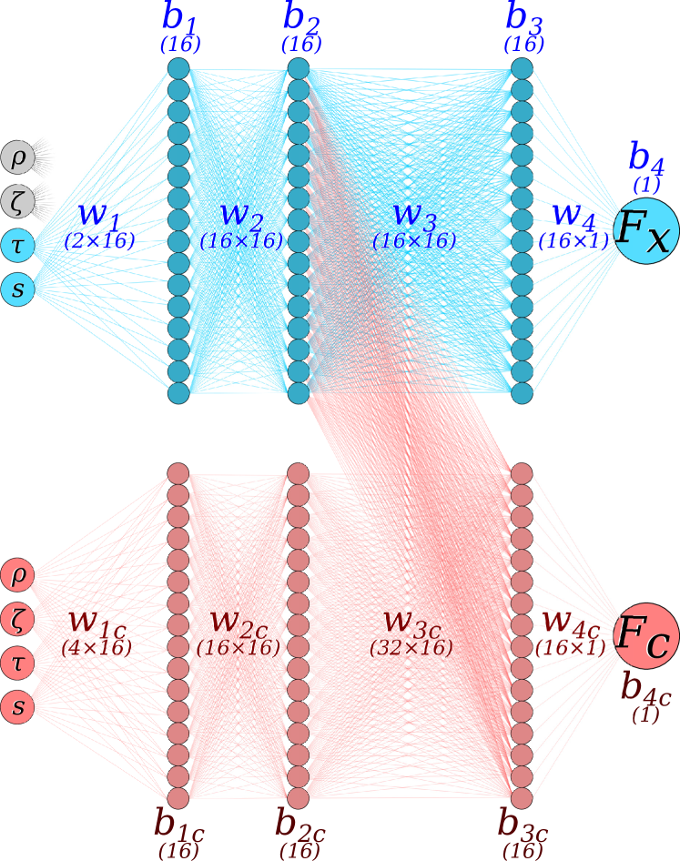
Figure 2: Architecture of the artificial neural network used in the present work. The w’s and $b$’s represent the weights and bias used on the feed-forward process and the products in parenthesis express the number of parameters in each of those elements.

2.2 Training of the Neural Network Functional

2.2.1 Loss Function

The loss function is the sum of errors of adiabatic energy differences, atomization energies, and electron densities

$$\begin{split}\Delta_{\text{err}}=&\sum_{i}^{\textit{G2}}\left[\frac{1}{E_{0}}\big{|}AE_{i}^{\text{REF.}}-AE_{i}^{\text{DFT}}\big{|}+\right.\\ &\quad\left.+\frac{1}{N_{i}}\int\big{|}\rho_{i}^{\text{REF.}}-\rho_{i}^{\text{DFT}}\big{|}dV\right]+\\ &\sum_{j}^{\textit{TMC}}\left[\frac{1}{E_{0}}\big{|}\Delta E_{\text{H-L},j}^{\textup{REF.}}-\Delta E_{\text{H-L},j}^{\textup{DFT}}\big{|}+\right.\\ &\quad\left.\frac{1}{N_{j}}\int\left(\big{|}\rho_{\text{H},j}^{\textup{REF.}}-\rho_{\text{H},j}^{DFT}\big{|}+\big{|}\rho_{\text{L},j}^{\textup{REF.}}-\rho_{\text{L},j}^{\textup{DFT}}\big{|}\right)dV\right],\end{split}$$ (7)

where the first summation is performed over three small molecules (NO, H2O, NH3) taken from the original G2 set with experimental reference values of atomization energies, $AE^{\textup{REF.}}$, extracted from Curtiss et al. ⁵⁰. To avoid confusion, from now on italic G2 refers to this set of three molecules, while the (non-italic) G2 refers to the complete set by Curtiss et al. ⁵⁰.

The second summation is performed over three diatomic transition metal complexes (TMC) with reference values for adiabatic energy difference, $\Delta E_{H-L}^{\textup{REF.}}$, taken from experiments and close to the CCSD(T) values within $0.02\text{\,}\mathrm{eV}$⁵⁷. These molecules are FeO, CuF, CrH. The error in the density for both the G2 set and the TMC is computed using the $L^{2}$ metric, by taking the CCSD(T) reference for the electronic density. Finally, $E_{0}=1$ Hartree, and $N_{j}$ is the number of electrons in the system $j$, both used to make the loss function dimensionless.

In order to evaluate the effects of the database, six different training sets were considered: G2 ([NO + H2O + NH3]), G2+FeO, G2+CuF, G2+CrH, TMC ([FeO + CuF + CrH]), and ALL (G2 + TMC). The terms of the loss function only apply when at least one of the related molecules is present in the training set. The Spearman correlation matrices and the principal component analysis of the loss function terms during the optimization are shown in the SI (Figures S2-S19).

The inclusion of the first term in eq. 7 was shown to yield good results for energetics of light element-molecules ^{36, 37}. Besides, it was shown that training sets with different types of data per sample (i.e., sparse training data) can significantly improve the performance of a machine learned-density functional⁵⁸.

The experimental values of $\Delta E_{H-L}$ are $1.81\text{\,}\mathrm{eV}$ for CuF (spin change: $S=1\to 3$),^{59, 60} $0.14\text{\,}\mathrm{eV}$ for FeO ($S=5\to 7$),⁶¹ and $-1.39\text{\,}\mathrm{eV}$ for CrH ($S=4\to 6$) ^{62, 63}. The choice of these specific molecules is done after considering four points: (i) the values of $\Delta E_{H-L}$ span a large range from negative to positive values, (ii) the diversity in terms of composition, (iii) the adiabatic energy difference involves different spin states in each case, and (iv) the configuration interaction weight of the dominant electronic configuration computed using CASSCF is different in the three cases pointing to different degrees of static correlations ($C_{0}^{2}=0.810$, $0.783$, and $0.938$; for CuF, FeO, and CrH respectively)⁶⁴. We do not claim here that our approach is capable to treat systems with multiconfigurational character. Rather, that the ANN-DFT yields a solution similar to the coupled cluster one, which gives an excellent agreement with experiment for these molecules ⁵⁷.

2.2.2 Optimization Algorithm

Since the equilibrium energies and densities are computed after converging the SCF process with a given set of parameters, the loss function depends on quantities that are related in a non-trivial way to the parameters of the ANN-functional. Thus, optimizing the parameters using a gradient based approach, although possible, as shown by Dick et al. and coworker³⁶, may be impractical in general. Recent studies have shown that non-gradient based optimization techniques can outperform gradient-based approaches for complicated loss functions ⁴⁶. Here, an adaptation of Particle Swarm Optimization (PSO)⁴⁵ is used as the training algorithm. PSO is built over a bio-inspired meta-heuristic: solutions (points on the parameters space of our neural network) will be treated as particles in a swarm (a collection of solutions) that forage for resources (that search for the minima of the loss function). The application of the PSO algorithm to the problem of functional optimization is shown in the flowchart of Figure 3(a). In the initial step, a search region in the parameters space is defined, and a swarm of particles with positions $\mathbf{x}_{i}(t=0)$ is randomly generated. These are initialized with velocities $\mathbf{v}_{i}(t=0)=0$ in this space. At each step $t$ in the PSO evolution, all the particles are submitted to a collective loss function evaluation. From this, the best solution ever visited by the swarm $\mathbf{x}_{\textup{best}}(t)$ and the best solution ever visited by the each particle $\mathbf{x}_{i,\textup{best}}(t)$ are saved. The velocities and positions on the swarm at t+1 are then updated as follows:

$$\begin{split}\mathbf{v}_{i}(t+1)=&\quad\omega\mathbf{v}_{i}(t)\\ &+c_{1}\textup{Rand}{(0,1]}(\mathbf{x}_{i,\textup{best}}(t)-\mathbf{x}_{i}(t))\\ &+c_{2}\textup{Rand}{(0,1]}(\mathbf{x}_{\textup{best}}(t)-\mathbf{x}_{i}(t)),\end{split}$$ (8)

$$\mathbf{x}_{i}(t+1)=\mathbf{x}_{i}(t)+\mathbf{v}_{i}(t+1),$$ (9)

where $\textup{Rand}{(0,1]}$ are random numbers independently generated in the ${(0,1]}$ interval and $\omega$, $c_{1}$, and $c_{2}$ are constants that dictate the behavior of the particles on the swarm. $\omega$ mimics the inertia of a flying particle and is associated with the pink component of the velocity in Figure 3(b). $c_{1}$ gives to the particle a velocity component that points toward the best solution known by the particle itself and it is the red component in Figure 3(b). $c_{2}$ gives a velocity component that points toward the best solution known by the swarm, which implements the concept of collective intelligence and it is shown by the blue component in Figure 3(b).

The standard PSO approach⁴⁵ is modified here by changing the search region between PSO runs as described below. This solves the observed instability when trying to evaluate the loss function in points that are too far from solutions that we know already. At the beginning of the optimization process, the particles are initialized inside a box of size $s$ around the origin ($\varepsilon_{x/c}=F_{x/c}(0)\times\varepsilon_{x/c}^{\textup{R2SCAN}}=\varepsilon_{x/c}^{\textup{R2SCAN}}$). Once a given number of PSO steps is done, the searching box is moved so that its center corresponds to the best solution found until then as shown in Figure 3(c). The particles are redistributed and the PSO search restarts. The PSO steps are performed using $c_{1}=0.1$, $c_{2}=0.2$, and $\omega=0.1$. The search box in each migration is defined using $s=0.05$ (with periodic boundary conditions) and $10$ PSO steps are taken in each migration. A total of $32$ particles are used in each step and a total of $50$ migrations is performed for every run.

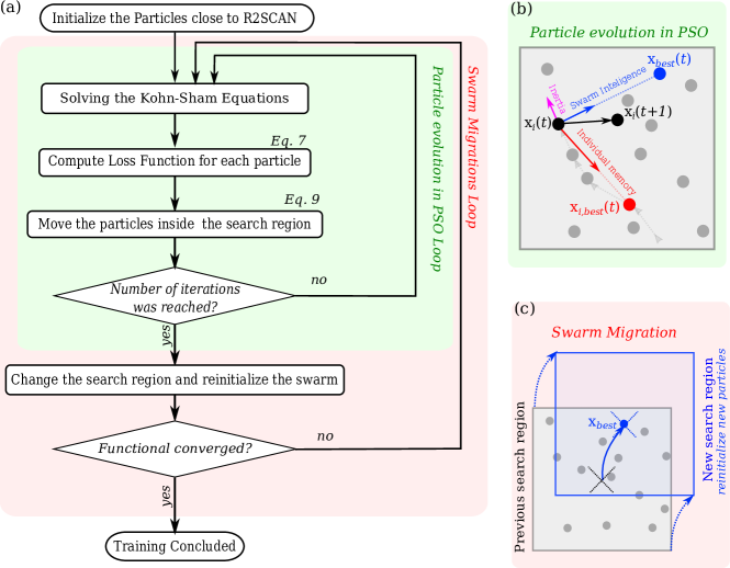
Figure 3: (a) Flowchart for the functional training approach as described in the text, including the PSO loop (green) and the migrations scheme (red). (b) Schematic representation of a PSO step. Magenta, red and blue vectors are associated with the right-hand side terms of equation 8, respectively. (c) Migration of the search region: all particles (grey and blue circles) are removed from the previous box (grey square) and reinitialized randomly inside a new one (blue square).

2.3 Technical Details

Our functional is implemented using an adaptation of the xc_pcNN import provided by Nagai and co-workers:⁶⁵ the neural network architecture is changed to the one proposed here and the physical constraints and corrections were adapted to the case of R2SCAN (imported from libxc⁶⁶).

The training code is an in-house application developed in Python3, combining the functionalities of pyscf⁶⁷ and ase⁶⁸ to compute the DFT SCFs and pyswarm⁶⁹ to perform the optimization inside each migration during the training process. For each particle (each parametrization of the ANN-DFT) the SCF is performed in order to compute the loss function. For this we use the 6-311++G(3df,3pd) for G2 and the ccpcvtz basis set for the transition metal complexes. The number of iterations within the SCF is set to 50 and the convergence criteria on the energy change is set to $10^{-6}E_{\textup{h}}$. The calculations that failed to converge within this criterion were not considered during the optimization process.

The reference densities are obtained via orbital optimized-CCSD(T), as implemented in ORCA 5.0⁷⁰. All the validations on the transition metal complexes are performed using pyscf and ccpcvtz. The validation on the whole G2 set of molecules is (shown in section S4 the SI) use geometries form ase.collections.g2 and the 6-311++G(3df,3pd) basis set.

3 Results

3.1 Trainings

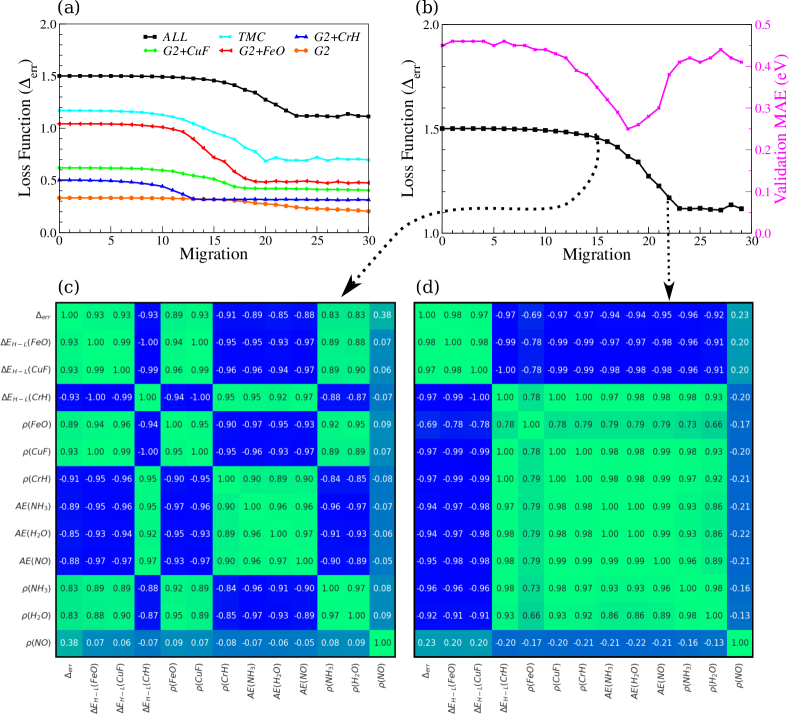
Figure 4: (a) Evolution of the loss function values during the training process, for the six different training sets considered here. (b) Comparison between the evolution of the loss function and that of the performance in the validation test along the migrations in the training with the complete ALL training set. (c) and (d) show Spearman’s rank correlation coefficients between the total loss function and each one of the $L^{1}$ distances that compose it. The two correspond, respectively, to the samples visited along migrations #$15$ and #$22$. The correlation matrix has converted in a heatmap.

In Figure 4(a), the evolution of the loss function, as defined in eq. 7 is drawn, where only the best solution (particle) at each migration is reported. After $30$ migrations, the solution is converged for every run except for G2. For this training set, a monotonic decrease of the loss function is observed until $36$ migrations. A different behavior is observed for the training sets including TMC, where the slow monotonic decrease is followed by a sharp decrease, and then by a stationary region. This change in behavior is associated with solutions that cannot be improved via migrations.

The training for the G2 follows path of error reduction of the atomization energy at the expense of a small increase in the error of the density (see Figures S2-S3). The loss function stops decreasing after migration $36$ and this is associated to a limit in the error of the atomization energy for NO and H2O. When the transition metal complexes are included in the training, a fast optimization of the adiabatic energy difference is observed simultaneously with the corresponding densities, highlighting the role of accurate electronic densities in the evaluation of adiabatic energy differences^{17, 31}. This is seen in the Spearman correlation matrices computed during the optimization for the first 2000 functionals visited for the G2+FeO training (see Figure S6) and for the ALL training for FeO and CuF (see Figure S15). In these training runs (when one or more transition metal complexes are included), the stationary region is associated with one of the $\Delta E_{H-L}$ reaching limit accuracy (i.e., the error associated to this quantity reaches zero). After this point, the process searches ways to optimize the other degrees of freedom (densities or atomization energies) and this leads to an increased dispersion on the error values associated with the $\Delta E_{H-L}$.

Figures 4(c) and (d) report the heatmap for the Spearman correlation matrix between the partial errors that compose the loss function for particles sampled at migration #$15$, i.e. during the optimization, and at migration #$22$, where the optimization stops, for the ALL training. At migration #$15$, in Figure 4(c) we see that the errors on energies and densities of FeO and CuF, as well as the densities on the G2 molecules, are optimized simultaneously. The loss function part associated with $\Delta E_{H-L}^{\ce{CrH}}$ and $\rho_{\ce{CrH}}$ is negatively correlated with those values meaning that their error increase while the total loss function decreases.

In the case of the ALL and TMC training sets, $\Delta E_{H-L}^{\ce{CuF}}$ was the first to reach a converged value close to zero. At this point of the optimization, the particles dispersion was enough to allow to find a new optimizing path for $\Delta E_{H-L}^{\ce{FeO}}$, as seen in the top left green block in Figure 4(d) (positive correlation between these quantities and the total loss function). The second block in Figure 4(d) showing strong positive correlation is negatively correlated with $\Delta_{\textup{err}}$.

3.2 Validation

3.2.1 The performance on Fe complexes

A validation test is performed by computing the errors (MEA) with respect to the CASPT2/CC adiabatic energy difference reported by Mariano et al.³¹ This is shown in the magenta curve of Figure 4(b) where each point correspond to the best solution for each migration obtained using the ALL training (black curve of the same Figure). The error on the validation reaches a minimum at step #$18$ while the loss function still decreases. The functional that performs the best on the validation test is from now on called $ANN^{ALL}_{val}$, while the one that best performs on the loss function is $ANN^{ALL}_{lf}$. Table 1 gathers the $\Delta E$ computed using the seven ANN-functionals (from the six training sets along with the validation). The performance of other DFT functionals, together with two recent ANN-based functionals, the one from ref. ³² named hereafter NAS from Nagai–Akashi–Sugino, and the DM21 one³⁴, are also reported for comparison in table 1.

Table 1: Performance of the seven ANN-based exchange and correlation functionals in the prediction of the adiabatic energy differences of the validation set. HS corresponds to $S=2$ and LS to $S=0$. Other local, semilocal, hybrid and recent ANN-based functionals are also reported for comparison. The reference values are from CASPT2/CC calculations and are taken from ref. ³¹, as discussed in the text.

	$\Delta E_{\text{H-L}}$ (eV)
	PBE	SCAN	NASa	B3LYP	DM21	R2SCAN	PBE[U]b	$ANN^{ALL}_{lf}$	$ANN^{ALL}_{val}$	$ANN^{G2+CrH}$	$ANN^{G2+CuF}$	$ANN^{G2+FeO}$	$ANN^{G2}$	$ANN^{TMC}$	REF.c
[Fe(H2O)6]^2+	-1.17	-0.81	-0.74	-1.44	-0.63	-1.36	-1.50	-2.51	-1.83	-1.03	-2.52	-3.06	3.69	-1.36	-1.83
[Fe(NH3)6]^2+	-0.06	0.21	0.21	-0.58	0.26	-0.29	-0.44	-1.27	-0.71	-0.01	-1.27	-1.73	3.75	-0.29	-0.64
[Fe(NCH)6]^2+	1.14	0.89	0.90	-0.21	0.64	0.41	0.21	-0.39	0.08	0.64	-0.41	-0.79	3.77	0.41	-0.16
[Fe(PH3)6]^2+	2.69	2.09	2.21	0.62	2.24	1.91	1.81	2.05	1.94	1.89	2.08	2.16	0.78	1.90	2.54
[Fe(CO)6]^2+	3.63	2.86	2.93	1.25	2.35	2.58	2.64	2.42	2.50	2.60	2.43	2.36	3.05	2.57	2.02
[Fe(NCH)6]^2+	4.11	3.38	3.42	1.86	2.99	3.06	3.23	2.93	2.99	3.10	2.95	2.87	3.24	3.05	2.87
MAEc	0.92	0.79	0.80	0.70	0.61	0.46	0.44	0.41	0.25	0.62	0.42	0.61	2.83	0.46
a NAS is the functional obtained by R. Nagai, R. Akashi, and O. Sugino.32
b PBE[U] represents the use of Hubbard $U_{sc}$-corrected density in the PBE functional.31
c Reference values come from CASPT2/CC.31

The performance of PBE, PBE[U], SCAN, and B3LYP was already discussed in previous studies^{17, 31}. Here, consistent with previous results, MAE of $0.92$, $0.79$ and $0.70\text{\,}\mathrm{eV}$ are found. The values computed using the Hubbard-U density corrected scheme using linear-response values of $U$, named PBE[U], are also reported for comparison. These are taken from ref.³¹ where the method was shown to yield the smallest error among $19$ different density functional approaches. The PBE[U] associated MAE is $0.44\text{\,}\mathrm{eV}$, and larger errors are observed for TPSSh (MAE$=$$0.49\text{\,}\mathrm{eV}$), PBE0 (MAE$=$$0.64\text{\,}\mathrm{eV}$) and M06-2X (MAE$=$$2.41\text{\,}\mathrm{eV}$).

It is worth noting here that R2SCAN (MAE$=$$0.49\text{\,}\mathrm{eV}$) yields a significant improvement over SCAN (MAE$=$$0.79\text{\,}\mathrm{eV}$) in terms of $\Delta E$, with a performance close to PBE[U]. This can be related to the improved numerical stability of the former (see section S1.1 in the SI). The two ANN-based functionals developed recently^{32, 34} exhibit a performance worse than R2SCAN: the ANN-based DM21 using range separated hybrids yields MAE=$0.61\text{\,}\mathrm{eV}$; the NAS³² functional yields MAE$=$$0.80\text{\,}\mathrm{eV}$ which is similar to SCAN, consistent with the fact that it is built as a correction over SCAN to improve the performance of atomization energies of light molecules, like the ones in the G2/G3 dataset. It is important at this point to note that $ANN^{G2}$, trained here only on the G2 set (H2O, NH3, NO), is the worst performer with a MAE of $2.83\text{\,}\mathrm{eV}$. This shows a far worse performance than NAS which is trained on similar molecules, i.e. H2O, NH3, CH2. For atomization energies on the G2 dataset, NAS gives MAE=$0.156\text{\,}\mathrm{eV}$³⁷, while for SCAN MAE$=$$0.269\text{\,}\mathrm{eV}$; for $ANN^{G2}$ MAE=$0.072\text{\,}\mathrm{eV}$, while for R2SCAN MAE$=$$0.127\text{\,}\mathrm{eV}$ (see Figure SX). The improved description of the atomization energies for $ANN^{G2}$ at the expense of the performance on the adiabatic energy differences points to a possible overfitting.

This does not occur in the case of $ANN^{ALL}$: this functional yields an improved prediction of the adiabatic energy difference (MAE$=$$0.41\text{\,}\mathrm{eV}$) with only a marginal worsening for the atomization energies ($0.15\text{\,}\mathrm{eV}$, see Table S1).

Among all the developed functionals, ALL and G2+CuF yield the best results with an improvement over R2SCAN, with the former, i.e. being the best performer. In Table 1, the performance of $ANN^{ALL}_{lf}$ and $ANN^{ALL}_{val}$is displayed. While the validation set only includes octahedral Fe complexes involving a $S=0$ to $S=2$ spin state change, $ANN^{ALL}_{lf}$ should aim at a lager diversity in terms of transition metal cation, spin state, and electronic structure. $ANN^{ALL}_{val}$, with its low MAE of $0.25\text{\,}\mathrm{eV}$, showcases how our results can be biased towards a specific situation.

3.2.2 Generalization on other metallic complexes

Another set of molecules is now used with different types of transition metal atoms and varying local coordinations in order to evaluate the performance of $ANN^{ALL}_{lf}$ as compared to the biased $ANN^{ALL}_{val}$. Nine spin state splitting values from six molecular complexes are considered from the work of Pierloot et al. ^{71, 8}. This set contains Fe complexes, such as FeL2 and FeL2SH, in a square-planar and square-pyramidal configuration respectively, MnL2, the octahedral complex [Co(NCH)6]^2+, and the two organometallic complexes, MnCp_2, and NiCp(acac) (L2 being the bidendate C3N2H_5^-, Cp$=$cyclopentadienyl, acac$=$acetylacetonate).

The predictions for adiabatic energy differences obtained using $ANN^{ALL}_{lf}$ and $ANN^{ALL}_{val}$ is reported in Table 2 together with other known functionals such as TPSS, R2SCAN, PBE, PBE[U] and DM21. Coupled cluster-corrected CASPT2 (CASPTE/CC) values from Pierloot et al. are taken as here reference⁷¹.

Table 2: Performance of different exchange and correlation functionals for the prediction of adiabatic energy differences of the test set. Some spin configurations could not be converged depending on spin state and thus a few values from the table are missing, and marked as “-”.

		$\Delta E_{\text{H-L}}$ (eV)
	2S+1	$ANN^{ALL}_{lf}$	$ANN^{ALL}_{val}$	R2SCAN	TPSS	PBE	PBE[U]	DM21	REF.b
FeL2	$1\rightarrow 5$	-1.439	-0.944	-0.611	0.227	-	-1.096	-1.968	-1.487
	$3\rightarrow 5$	0.193	0.513	0.746	1.259	1.245	0.756	0.814	0.213
MnL2	$2\rightarrow 6$	-2.078	-1.427	-0.957	-0.055	-0.111	-0.961	-	-1.782
	$4\rightarrow 6$	-0.061	0.207	0.414	0.835	0.919	0.491	-0.739	-0.455
FeL2SH	$2\rightarrow 6$	-0.464	0.081	0.470	-0.416	1.087	-	-	0.399
	$4\rightarrow 6$	-0.488	-0.130	0.123	0.588	0.521	0.245	-	-0.017
[Co(NCH)6]2+	$2\rightarrow 4$	-0.372	-0.170	-0.027	0.31	0.476	0.165	0.057	-0.581
NiCp(acac)	$1\rightarrow 3$	-0.204	-0.177	-0.157	0.046	0.163	0.095	0.414	0.117
MnCp2	$2\rightarrow 6$	-0.220	-0.354	0.184	0.649	0.981	0.432	-	0.304
MAEb		0.349	0.406	0.474	0.945	0.885a	0.482a	0.460a
a Average computed over available values.
b Reference values come from CASPT2/CC.71

As shown above for the validation set, R2SCAN (MAE=0.474 eV) substantially improves over PBE (MAE=0.885 eV) and TPSS (MAE=0.945 eV). The best performers, $ANN^{ALL}_{lf}$ and $ANN^{ALL}_{val}$, further improve over R2SCAN with MAE of 0.349 eV and 0.406 eV, respectively. We note a better performance of DM21 (MAE=0.460 eV) for this set of molecules as compared with the octahedral complexes presented above. Yet, we note here that owing to the heavy architecture of the DM21 functional (it is defined pointwise using Hartree-Fock, range-separated hybrid and LDA energy densities with weights computed as ANN with hidden layers containing up to $256$ neurons), the calculation of adiabatic energy differences is costly and the SCF is sometimes difficult to converge. This is the case here where the SCF could not converge for MnL₂ ($2S+1=4\textup{ and }6$), FeL₂SH ($2S+1=2\textup{ and }4$), and MnCp₂ ($2S+1=6$) despite starting the calculation using an already converged density (R2SCAN here) as suggested in the DM21 documentation⁷².

Among the studied molecules, the square planar compounds MnL2 and FeL2 result in the largest error for R2SCAN of up to $0.9\text{\,}\mathrm{eV}$, a performance that is significantly improved by both the functionals trained with $ALL$. Also, a good performance is seen for $ANN^{ALL}_{lf}$ to describe complexes far from the training set in terms of geometry and choice of atoms, such as [Co(NCH)_6]^2+ (error of $0.21\text{\,}\mathrm{eV}$).

The curves shown in Figure 4(b) may convey the message of an over-fitting during the ALL training, as seen from the increase of the validation error. During the optimization on the training set, the performance for the chosen validation set gets worse after migration #18. Yet, the $ANN^{ALL}_{lf}$ functional outperforms $ANN^{ALL}_{val}$ in the generality test (see Table 2). The fact that the best fitted functional for the training set best performs also for the generality test implies a good transferability of the functional. This can be associated also to the physical limits imposed during the training.

4 Conclusion

The ANN-based exchange and correlation functional in DFT developed in this work outperforms most known local, semilocal, and meta-GGA functionals in the prediction of adiabatic energy differences for transition metal complexes. It is built as a physically-constrained meta-GGA artificial neural-network correction to R2SCAN and trained over a small dataset of electronic densities, atomization energies and/or adiabatic energy differences. Our results show a good performance of the non gradient-based bioinspired training algorithm PSO where the optimization can reach a hard limit, as in the case of the adiabatic energy differences of CuF, FeO, and CrH. Six functionals were obtained by using different subsets of the training molecules. The functional optimized by using the whole training set, $ANN^{ALL}_{lf}$ (MAE$=$$0.41\text{\,}\mathrm{eV}$), and that obtained using the $G2+CuF$, $ANN^{G2+CrF}$ (MAE$=$$0.42\text{\,}\mathrm{eV}$), yield a performance on the validation test superior to the best performer R2SCAN (MAE$=$$0.44\text{\,}\mathrm{eV}$). Such a validation test performed on octahedral iron complexes shows that our functional substantially improves over recent ANN-based functionals, such as the meta-GGA NAS and the range-separated hybrid DM21. The best performer on the validation test, $ANN^{ALL}_{lf}$, best performs also on the generality test with a MAE$=$$0.349\text{\,}\mathrm{eV}$. Finally, we show that by changing the the criteria used to select the functional (from the loss function itself to a validation metric), we were able to bias the results to improve the performance on a specific set of data. For example, the best performer on the validation test, named $ANN^{ALL}_{val}$, yields a MAE as small as $0.25\text{\,}\mathrm{eV}$, but the associated MAE on the generality test is larger (MAE$=$$0.41\text{\,}\mathrm{eV}$) than for the $ANN^{ALL}_{lf}$. Overall, the results of this study highlight the impact of machine learning approaches to enhance the accuracy of approximate density functional theory through the development of optimized functionals.

Computational resources were provided by the CINES and IDRIS under Project No. INP2227/72914, as well as CIMENT/GRICAD for computational resources. This work was performed within the framework of the Centre of Excellence of Multifunctional Architectured Materials CEMAM-ANR-10-LABX-44-01 funded by the “Investments for the Future” Program. This work has been partially supported by MIAI@Grenoble Alpes (ANR-19-P3IA-0003). The authors thank Lucia Reining for fruitful discussions. Discussions within the French collaborative network in artificial intelligence in materials science GDR CNRS 2123 (IAMAT) are also acknowledged.

Experimental procedures and characterization data for all new compounds. The class will automatically add a sentence pointing to the information on-line:

References

- Jones 2015 Jones, R. O. Density functional theory: Its origins, rise to prominence, and future. Rev. Mod. Phys. 2015, 87, 897–923
- Cohen et al. 2012 Cohen, A. J.; Mori-Sánchez, P.; Yang, W. Challenges for Density Functional Theory. Chem. Rev. 2012, 112, 289–320, PMID: 22191548
- Poloni et al. 2008 Poloni, R.; Machon, D.; Fernandez-Serra, M. V.; Le Floch, S.; Pascarelli, S.; Montagnac, G.; Cardon, H.; San-Miguel, A. High-pressure stability of . Phys. Rev. B 2008, 77, 125413
- Wilbraham et al. 2017 Wilbraham, L.; Verma, P.; Truhlar, D. G.; Gagliardi, L.; Ciofini, I. Multiconfiguration Pair-Density Functional Theory Predicts Spin-State Ordering in Iron Complexes with the same Accuracy as Complete Active Space Second-Order Perturbation Theory at a Significantly Reduced Computational Cost. J. Phys. Chem. Lett. 2017, 8, 2026–2030
- Domingo et al. 2010 Domingo, A.; Àngels Carvajal, M.; De Graaf, C. Spin Crossover in Fe(II) Complexes: An Ab Initio Study of Ligand -Donation. Int. J. Quantum Chem. 2010, 110, 331–337
- Radoń 2019 Radoń, M. Benchmarking Quantum Chemistry Methods for Spin-State Energetics of Iron Complexes Against Quantitative Experimental Data. Phys. Chem. Chem. Phys. 2019, 21, 4854–4870
- Swart 2008 Swart, M. Accurate Spin-State Energies for Iron Complexes. J. Chem. Theory Comput. 2008, 4, 2057–2066
- Phung et al. 2018 Phung, Q. M.; Feldt, M.; Harvey, J. N.; Pierloot, K. Toward highly Accurate Spin State Energetics in First-Row Transition Metal Complexes: A Combined CASPT2/CC Approach. J. Chem. Theory Comput. 2018, 14, 2446–2455
- Reimann and Kaupp 2023 Reimann, M.; Kaupp, M. Spin-State Splittings in 3d Transition-Metal Complexes Revisited: Toward a Reliable Theory Benchmark. J. Chem. Theory Comput. 2023, 19, 97–108, PMID: 36576816
- Molnár et al. 2019 Molnár, G.; Mikolasek, M.; Ridier, K.; Fahs, A.; Nicolazzi, W.; Bousseksou, A. Molecular Spin Crossover Materials: Review of the Lattice Dynamical Properties. Ann. Phys. 2019, 531, 1900076
- Kumar and Ruben 2017 Kumar, K. S.; Ruben, M. Emerging Trends in Spin Crossover (SCO) Based Functional Materials and Devices. Coordin Chem. Rev. 2017, 346, 176–205
- Resines-Urien et al. 2019 Resines-Urien, E.; Burzurí, E.; Fernandez-Bartolome, E.; García García-Tuñón, M. A.; de la Presa, P.; Poloni, R.; Teat, S. J.; Costa, J. S. A switchable iron-based coordination polymer toward reversible acetonitrile electro-optical readout. Chem. Sci. 2019, 10, 6612–6616
- Resines-Urien et al. 2020 Resines-Urien, E.; Piñeiro-López, L.; Fernandez-Bartolome, E.; Gamonal, A.; Garcia-Hernandez, M.; Sánchez Costa, J. Covalent post-synthetic modification of switchable iron-based coordination polymers by volatile organic compounds: a versatile strategy for selective sensor development. Dalton Trans. 2020, 49, 7315–7318
- Swart et al. 2004 Swart, M.; Groenhof, A. R.; Ehlers, A. W.; Lammertsma, K. Validation of Exchange-Correlation Functionals for Spin States of Iron Complexes. J. Phys. Chem. A 2004, 108, 5479–5483
- Pierloot and Vancoillie 2006 Pierloot, K.; Vancoillie, S. Relative Energy of the High- and Low- Spin States of [Fe(H2O)6]2+,[Fe(NH3)6]2+, and [Fe(bpy)3]2+: CASPT2 Versus Density Functional Theory. J. Chem. Phys. 2006, 125, 124303
- Droghetti et al. 2012 Droghetti, A.; Alfè, D.; Sanvito, S. Assessment of Density Functional Theory for Iron(II) Molecules Across the Spin-Crossover Transition. J. Chem. Phys. 2012, 137, 124303
- Song et al. 2018 Song, S.; Kim, M.-C.; Sim, E.; Benali, A.; Heinonen, O.; Burke, K. Benchmarks and Reliable DFT Results for Spin Gaps of Small Ligand Fe(II) Complexes. J. Chem. Theory Comput. 2018, 14, 2304–2311
- Fouqueau et al. 2005 Fouqueau, A.; Casida, M. E.; Daku, L. M. L.; Hauser, A.; Neese, F. Comparison of Density Functionals for Energy and Structural Differences Between the High- and Low- Spin States of Iron(II) Coordination Compounds. II. More Functionals and the Hexaminoferrous Cation, [Fe(NH3)6]2+. J. Chem. Phys. 2005, 122, 044110
- Radoń 2014 Radoń, M. Revisiting the Role of Exact Exchange in DFT Spin-State Energetics of Transition Metal Complexes. Phys. Chem. Chem. Phys. 2014, 16, 14479–14488
- Mortensen and Kepp 2015 Mortensen, S. R.; Kepp, K. P. Spin Propensities of Octahedral Complexes from Density Functional Theory. J. Phys. Chem. A 2015, 119, 4041–4050
- Ioannidis and Kulik 2015 Ioannidis, E. I.; Kulik, H. J. Towards Quantifying the Role of Exact Exchange in Predictions of Transition Metal Complex Properties. J. Chem. Phys. 2015, 143, 034104
- Kulik 2015 Kulik, H. J. Perspective: Treating Electron Over-Delocalization with the DFT+ Method. J. Chem. Phys. 2015, 142, 240901
- Rehier et al. 2001 Rehier, M.; Salomon, O.; Arthus Hess, B. Reparameterization of Hybrid Functionals Based on Energy Differences of States of Different Multiplicit. Theor. Chem. Acc. 2001, 107, 48–55
- Prokopiou and Kronik 2018 Prokopiou, G.; Kronik, L. Spin-State Energetics of Fe Complexes from an Optimally Tuned Range-Separated Hybrid Functional. Chem.-Eur. J. 2018, 24, 5173–5182
- Kulik et al. 2006 Kulik, H. J.; Cococcioni, M.; Scherlis, D. A.; Marzari, N. Density Functional Theory in Transition-Metal Chemistry: A Self-Consistent Hubbard Approach. Phys. Rev. Lett. 2006, 97, 103001
- Scherlis et al. 2007 Scherlis, D. A.; Cococcioni, M.; Sit, P.; Marzari, N. Simulation of Heme Using DFT+U: A Step toward Accurate Spin-State Energetics. J. Phys. Chem. B 2007, 111, 7384–7391, PMID: 17547444
- Kulik and Marzari 2010 Kulik, H. J.; Marzari, N. Systematic Study of First-Row Transition-Metal Diatomic Molecules: A Self-Consistent DFT+ Approach. J. Chem. Phys. 2010, 133, 114103
- Vela et al. 2020 Vela, S.; Fumanal, M.; Cirera, J.; Ribas-Arino, J. Thermal Spin Crossover in Fe(ii) and Fe(iii). Accurate Spin State Energetics at the Solid State. Phys. Chem. Chem. Phys. 2020, 22, 4938–4945
- Albavera-Mata et al. 2022 Albavera-Mata, A.; Trickey, S. B.; Hennig, R. G. Mean Value Ensemble Hubbard-U Correction for Spin-Crossover Molecules. J. Phys. Chem. Letters 2022, 13, 12049–12054, PMID: 36542415
- Mariano et al. 2020 Mariano, L. A.; Vlaisavljevich, B.; Poloni, R. Biased Spin-State Energetics of Fe(II) Molecular Complexes within Density-Functional Theory and the Linear-Response Hubbard U Correction. J. Chem. Theory and Comput. 2020, 16, 6755–6762, PMID: 33108722
- Mariano et al. 2021 Mariano, L. A.; Vlaisavljevich, B.; Poloni, R. Improved Spin-State Energy Differences of Fe (II) molecular and crystalline complexes via the Hubbard U-corrected Density. Journal of Chemical Theory and Computation 2021, 17, 2807–2816
- Nagai et al. 2022 Nagai, R.; Akashi, R.; Sugino, O. Machine-learning-based exchange correlation functional with physical asymptotic constraints. Physical Review Research 2022, 4, 013106
- Li et al. 2021 Li, L.; Hoyer, S.; Pederson, R.; Sun, R.; Cubuk, E. D.; Riley, P.; Burke, K., et al. Kohn-Sham equations as regularizer: Building prior knowledge into machine-learned physics. Physical Review Letters 2021, 126, 036401
- Kirkpatrick et al. 2021 Kirkpatrick, J.; McMorrow, B.; Turban, D. H.; Gaunt, A. L.; Spencer, J. S.; Matthews, A. G.; Obika, A.; Thiry, L.; Fortunato, M.; Pfau, D., et al. Pushing the frontiers of density functionals by solving the fractional electron problem. Science 2021, 374, 1385–1389
- King et al. 2021 King, D. S.; Truhlar, D. G.; Gagliardi, L. Machine-learned energy functionals for multiconfigurational wave functions. The Journal of Physical Chemistry Letters 2021, 12, 7761–7767
- Dick and Fernandez-Serra 2021 Dick, S.; Fernandez-Serra, M. Highly accurate and constrained density functional obtained with differentiable programming. Phys. Rev. B 2021, 104, L161109
- Nagai et al. 2020 Nagai, R.; Akashi, R.; Sugino, O. Completing density functional theory by machine learning hidden messages from molecules. npj Computational Materials 2020, 6
- Chen et al. 2020 Chen, Y.; Zhang, L.; Wang, H.; E, W. Deepks: A comprehensive data-driven approach toward chemically accurate density functional theory. Journal of Chemical Theory and Computation 2020, 17, 170–181
- Dick and Fernandez-Serra 2020 Dick, S.; Fernandez-Serra, M. Machine learning accurate exchange and correlation functionals of the electronic density. Nature Communications 2020, 11, 3509
- Nagai et al. 2018 Nagai, R.; Akashi, R.; Sasaki, S.; Tsuneyuki, S. Neural-network Kohn-Sham exchange-correlation potential and its out-of-training transferability. The Journal of Chemical Physics 2018, 148, 241737
- Brockherde et al. 2017 Brockherde, F.; Vogt, L.; Li, L.; Tuckerman, M. E.; Burke, K.; Müller, K.-R. Bypassing the Kohn-Sham equations with machine learning. Nature Communications 2017, 8, 872
- Li et al. 2016 Li, L.; Snyder, J. C.; Pelaschier, I. M.; Huang, J.; Niranjan, U.-N.; Duncan, P.; Rupp, M.; Müller, K.-R.; Burke, K. Understanding machine-learned density functionals. International Journal of Quantum Chemistry 2016, 116, 819–833
- Snyder et al. 2012 Snyder, J. C.; Rupp, M.; Hansen, K.; Müller, K.-R.; Burke, K. Finding density functionals with machine learning. Physical Review Letters 2012, 108, 253002
- Kalita et al. 2021 Kalita, B.; Li, L.; McCarty, R. J.; Burke, K. Learning to approximate density functionals. Accounts of Chemical Research 2021, 54, 818–826
- Kennedy and Eberhart 1995 Kennedy, J.; Eberhart, R. Particle swarm optimization. Proceedings of ICNN’95-International Conference on Neural Networks. 1995; pp 1942–1948
- Tian and Ha 2022 Tian, Y.; Ha, D. Modern evolution strategies for creativity: Fitting concrete images and abstract concepts. International Conference on Computational Intelligence in Music, Sound, Art and Design (Part of EvoStar). 2022; pp 275–291
- Kohn and Sham 1965 Kohn, W.; Sham, L. J. Self-Consistent Equations Including Exchange and Correlation Effects. Phys. Rev. 1965, 140, A1133–A1138
- Furness et al. 2020 Furness, J. W.; Kaplan, A. D.; Ning, J.; Perdew, J. P.; Sun, J. Accurate and Numerically Efficient r2SCAN Meta-Generalized Gradient Approximation. The Journal of Physical Chemistry Letters 2020, 11, 8208–8215
- Sun et al. 2015 Sun, J.; Ruzsinszky, A.; Perdew, J. P. Strongly constrained and appropriately normed semilocal density functional. Physical Review Letters 2015, 115, 036402
- Curtiss et al. 1997 Curtiss, L. A.; Raghavachari, K.; Redfern, P. C.; Pople, J. A. Assessment of Gaussian-2 and density functional theories for the computation of enthalpies of formation. The Journal of Chemical Physics 1997, 106, 1063–1079
- Furness and Sun 2019 Furness, J. W.; Sun, J. Enhancing the efficiency of density functionals with an improved iso-orbital indicator. Physical Review B 2019, 99, 041119
- Yang et al. 2016 Yang, Z.-h.; Peng, H.; Sun, J.; Perdew, J. P. More realistic band gaps from meta-generalized gradient approximations: Only in a generalized Kohn-Sham scheme. Physical Review B 2016, 93, 205205
- Sitkiewicz et al. 2022 Sitkiewicz, S. P.; Zalesńy, R.; Ramos-Cordoba, E.; Luis, J. M.; Matito, E. How reliable are modern density functional approximations to simulate vibrational spectroscopies? The Journal of Physical Chemistry Letters 2022, 13, 5963–5968
- Bartók and Yates 2019 Bartók, A. P.; Yates, J. R. Regularized SCAN functional. The Journal of Chemical Physics 2019, 150, 161101
- Levy and Perdew 1985 Levy, M.; Perdew, J. P. Hellmann-Feynman, virial, and scaling requisites for the exact universal density functionals. Shape of the correlation potential and diamagnetic susceptibility for atoms. Physical Review A 1985, 32, 2010
- Oliver and Perdew 1979 Oliver, G.; Perdew, J. Spin-density gradient expansion for the kinetic energy. Physical Review A 1979, 20, 397
- Kulik and Marzari 2010 Kulik, H. J.; Marzari, N. Systematic study of first-row transition-metal diatomic molecules: A self-consistent DFT+U approach. The Journal of Chemical Physics 2010, 133, 114103
- Kasim and Vinko 2021 Kasim, M. F.; Vinko, S. M. Learning the Exchange-Correlation Functional from Nature with Fully Differentiable Density Functional Theory. Phys. Rev. Lett. 2021, 127, 126403
- Dufour et al. 1982 Dufour, C.; Schamps, J.; Barrow, R. Electronic states of the CuF molecule. II. Nature of the observed states. Journal of Physics B: Atomic and Molecular Physics (1968-1987) 1982, 15, 3819
- Brazier et al. 1983 Brazier, C. R.; Brown, J. M.; Purnell, M. R. Nuclear hyperfine splittings for copper monofluoride in the a3+ state. Journal of Molecular Spectroscopy 1983, 99, 279–287
- Drechsler et al. 1997 Drechsler, G.; Boesl, U.; BäSmann, C.; Schlag, E. Mass selected anion-zero kinetic energy photoelectron spectroscopy (anion-ZEKE): Ground and low excited states of FeO. The Journal of Chemical Physics 1997, 107, 2284–2291
- Miller et al. 1987 Miller, A. E. S.; Feigerle, C. S.; Lineberger, W. C. Laser photoelectron spectroscopy of \ceCrH-, \ceCoH-, and \ceNiH-: Periodic trends in the electronic structure of the transition‐metal hydrides. The Journal of Chemical Physics 1987, 87, 1549–1556
- Ram et al. 1993 Ram, R.; Jarman, C.; Bernath, P. Fourier transform emission spectroscopy of the A6+-X6+ system of CrH: evidence for a 4+ lowest excited state. Journal of Molecular Spectroscopy 1993, 161, 445–454
- Jiang et al. 2012 Jiang, W.; DeYonker, N. J.; Wilson, A. K. Multireference Character for 3d Transition-Metal-Containing Molecules. Journal of Chemical Theory and Computation 2012, 8, 460–468, PMID: 26596596
- 65 (ml-electron project), R. N. PySCF version of physically constrained NN-based XC functional. \urlhttps://github.com/ml-electron-project/pcNN_mol
- Lehtola et al. 2018 Lehtola, S.; Steigemann, C.; Oliveira, M. J.; Marques, M. A. Recent developments in libxc—A comprehensive library of functionals for density functional theory. SoftwareX 2018, 7, 1–5
- Sun et al. 2020 Sun, Q.; Zhang, X.; Banerjee, S.; Bao, P.; Barbry, M.; Blunt, N. S.; Bogdanov, N. A.; Booth, G. H.; Chen, J.; Cui, Z.-H., et al. Recent developments in the PySCF program package. The Journal of Chemical Physics 2020, 153, 024109
- Larsen et al. 2017 Larsen, A. H.; Mortensen, J. J.; Blomqvist, J.; Castelli, I. E.; Christensen, R.; Dułak, M.; Friis, J.; Groves, M. N.; Hammer, B.; Hargus, C., et al. The atomic simulation environment—a Python library for working with atoms. Journal of Physics: Condensed Matter 2017, 29, 273002
- Miranda 2018 Miranda, L. J. V. PySwarms: a research toolkit for Particle Swarm Optimization in Python. The Journal of Open Source Software 2018, 3, 433
- Neese et al. 2020 Neese, F.; Wennmohs, F.; Becker, U.; Riplinger, C. The ORCA quantum chemistry program package. The Journal of Chemical Physics 2020, 152, 224108
- Pierloot et al. 2017 Pierloot, K.; Phung, Q. M.; Domingo, A. Spin State Energetics in First-Row Transition Metal Complexes: Contribution of (3s3p) Correlation and its Description by Second-Order Perturbation Theory. J. Chem. Theory Comput. 2017, 13, 537–553
- 72 DeepMind, DM21 Interface for PySCF. \urlhttps://github.com/deepmind/deepmind-research/tree/master/density_functional_approximation_dm21