Time-series Anomaly Detection via Contextual Discriminative Contrastive Learning

Abstract

Detecting anomalies in temporal data is challenging due to anomalies being dependent on temporal dynamics. One-class classification methods are commonly used for anomaly detection tasks, but they have limitations when applied to temporal data. In particular, mapping all normal instances into a single hypersphere to capture their global characteristics can lead to poor performance in detecting context-based anomalies where the abnormality is defined with respect to local information. To address this limitation, we propose a novel approach inspired by the loss function of DeepSVDD. Instead of mapping all normal instances into a single hypersphere center, each normal instance is pulled toward a recent context window. However, this approach is prone to a representation collapse issue where the neural network that encodes a given instance and its context is optimized towards a constant encoder solution. To overcome this problem, we combine our approach with a deterministic contrastive loss from Neutral AD, a promising self-supervised learning anomaly detection approach. We provide a theoretical analysis to demonstrate that the incorporation of the deterministic contrastive loss can effectively prevent the occurrence of a constant encoder solution. Experimental results show superior performance of our model over various baselines and model variants on real-world industrial datasets.

1 Introduction

Time series anomaly detection is a critical tool in industrial applications, helping to detect abnormal behavior in complex systems and prevent costly failures. With the rise of data-driven industries, identifying anomalous patterns in real-time monitoring and analysis of sensor data is becoming increasingly important. By detecting anomalies, industries can improve production efficiency, reduce downtime, and enhance the safety and reliability of their systems.

Detecting anomalies in temporal data presents unique challenges compared to traditional anomaly detection tasks, as anomalies in temporal data are often context-dependent, meaning that they are contingent upon the temporal dynamics of the system. As shown in Figure 1, anomalies in temporal data may occur within normal value ranges, but they represent events that deviate from their expected behavior given the dynamic temporal context in which they occur. Thus, an effective time series anomaly detection method needs to capture the context-aware nature of anomalies and the temporal dependencies within the data.

One-class classification methods are widely used in anomaly detection tasks, with the objective of learning a model of normal data and identifying anomalies as data points outside this model. Examples of these methods include Support Vector Data Description (SVDD) [29] and one-class SVM [25], which respectively construct a hypersphere or a hyperplane around the normal data. However, such methods are computationally expensive in dealing with complex data structures and high-dimensional data, and often require substantial feature engineering. To address these challenges, deep learning-based one-class classification methods have been developed to learn more complex representations of normal data. One popular method in this category is DeepSVDD [23], which employs a deep neural network to map the input data into a high-dimensional feature space and learns a hypersphere that encapsulates the normal data.

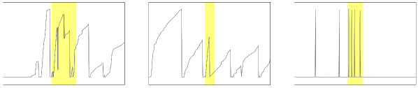
Figure 1: The figure presents several examples of time series segments from a real-world industrial dataset, with anomalies highlighted in yellow. Contextual information plays a crucial role in identifying these anomalies.

While one-class classification methods have demonstrated success in detecting anomalies in various scenarios such as computer vision, they exhibit a tendency to map all data points to a single center point or region in the feature space, which limits their efficacy in detecting anomalies in time series data. This is particularly relevant as time series data often display intricate and nonlinear temporal patterns, and the majority of anomalies in time series data are context-specific, i.e., they deviate from recent past observations. Consequently, a single global representation of normal behavior may not be able to fully capture the complex and context-specific nature of anomalies in time series data.

Recent research has proposed several approaches to extend DeepSVDD for time series anomaly detection. For instance, COUTA [33] and COCA [30] use TCNs and LSTMs, respectively, to capture temporal patterns in time series data, while OCPAE [35] incorporates time series forecasting and sequence reconstruction objectives along with a one-class classification objective to account for local temporal dependencies. However, these methods still has the limitation of mapping all latent representations of normal instances into a single hypersphere. In contrast, THOC [26] uses a dilated RNN with skip connections to encode time series data, and clusters features from all intermediate layers into multiple clusters, allowing for the representation of normal behaviors by multiple hyperspheres. However, selecting the appropriate number of $k$ centers remains a challenge.

In this work, we propose a novel adaptation based on the original loss function of DeepSVDD. Instead of converging all normal instances towards a single center, we propose a contextual-based loss function that pulls the latent representation of each instance towards that of its nearby context sequence. The underlying assumption is that nearby sequences should share similar latent representations, while anomalous instances should exhibit significant dissimilarity from their neighbors. This approach enables more precise identification of anomalous instances than traditional one-class methods, which often fail to account for the temporal characteristics and contextual nature of anomalies.

However, our proposed approach, like DeepSVDD, may be susceptible to a representation collapse issue, where the neural network encoding a given instance and its context may be optimized towards a constant encoder solution. To address this issue, we augment our approach with a deterministic contrastive loss from the recent self-supervised learning-based anomaly detection approach, Neural AD [21], which has demonstrated success in various data types. The deterministic contrastive loss applies regularizations to the transformations of an input sequence to guarantee diverse and semantically meaningful latent representations of the sequences.

In summary, our contributions are threefold:

1. We propose a novel anomaly detection framework that considers the contextual nature of temporal anomalies through a combination of contextual contrastive loss and deterministic contrastive loss.

2. We provide theoretical analysis demonstrating that a combination of the two losses effectively mitigates the representation collapse problem.

3. We conduct extensive experiments on real-world industrial datasets, including comparison studies, ablation studies, and visual analysis, that demonstrate the superior performance of our proposed approach over various baseline methods and variants of our model.

2 Preliminary

In this section, we provide a brief review of two methods closely related to our work, DeepSVDD and Neutral AD.

2.1 DeepSVDD

DeepSVDD is an unsupervised learning method that aims to learn a compact representation of the normal class using a neural network encoder. Specifically, under the semi-supervised setting where the majority of training data are assumed to be normal instances, DeepSVDD seeks to map all instances into a hypersphere of minimum volume. This is achieved by minimizing the following objective function:

$$\min_{\theta,c}\frac{1}{N}\sum^{N}_{i=1}\|\phi(x_{i};\theta)-c\|^{2}_{2}+\lambda\Omega(\theta),$$ (1)

where $x_{i}$ denotes the $i$-th instance out of $N$ training samples, $\phi(\cdot)$ is a neural network with parameter $\theta$ that encodes a given input into its latent representation, and $c$ represents the center of the hypersphere. The regularization term, $\lambda\Omega(\theta)$, typically takes the form of an $l_{2}$ regularization, which encourages the model’s weights to be small and reduces the model’s complexity. The selection of the center $c$ in the objective function is crucial to prevent a hypersphere collapse issue, which occurs when all instances are simply mapped to a constant.

2.2 NeuTral AD

The idea of NeuTral AD is inspired by the recent progress of self-supervised learning techniques that are primarily intended for anomaly detection in vision domain. These techniques adopt an augmentation prediction approach that generates a set of samples by applying various data augmentation operations to input images, training a model to classify the specific augmentation corresponding to an augmented sample [7], [9], and [31]. However, majority of them rely on hand-crafted transformations specialized for image data, making it challenging to design such transformations for data beyond images. To overcome this challenge, NeuTral AD [21] employs learnable transformations to embed transformed data into a semantic space that maintains the similarity of the transformed data to their original form while enabling easy differentiation between different transformations via separation in the representation space.

The NeuTral AD approach utilizes a determinative contrastive loss to enable the use of learnable transformations. Given an input sample $x$, the loss is defined as:

$${\mathcal{L}}=-\sum^{K}_{k=1}\log\frac{h(x^{k},x^{0})}{h(x^{k},x^{0})+\sum_{l\neq k}h(x^{k},x^{l})}$$ (2)

Here, $h(x^{k},x^{l})$ is defined as:

$$h(x^{k},x^{l})=\text{exp}(\text{sim}(f_{\phi}(x^{k}),f_{\phi}(x^{l}))/\tau)$$ (3)

$$x^{k}=T_{k}(x)$$ (4)

where $\tau$ is a hyperparameter called temperature, $\text{sim}(\cdot,\cdot)$ computes the cosine similarity between two inputs, $T_{k}(\cdot)$ is the $k^{th}$ transformation function that maps the original data into a different subspace of the same dimension as the input (e.g., via an MLP), $T_{0}(\cdot)$ is an identity function, $K$ is the number of learnable transformations, and $f_{\phi}(\cdot)$ is an encoder network that extracts latent information from different transformed inputs.

3 Related Works

This section primarily focuses on reviewing deep learning-related methods in anomaly detection due to the rapid advances in deep learning approaches.

The two mainstream deep time series anomaly detection approaches are forecasting-based and reconstruction-based methods. Forecasting-based methods predict future values and identify anomalies as data points deviating from predictions. Reconstruction-based methods reconstruct input data and identify anomalies as data points that cannot be accurately reconstructed. Recent works [10] [6] [37] [8] for forecasting-based methods leverage various neural network architectures like LSTMs, GRUs, TCNs, GNNs, and hybrid combinations. Reconstruction-based methods include deep autoencoders (AEs) [28] [16] [19] [36] and Generative Adversarial Networks (GANs) [2] [15] with varying underlying sequence encoder architectures.

Other promising approaches for time series anomaly detection include the aforementioned one-class classification methods and self-supervised learning methods. Self-supervised learning techniques can be divided into two categories: augmentation prediction-based (See details in Section 2.2) and contrastive learning-based approaches. Contrastive learning brings together representations of data instances and their augmented versions while pushing away negative samples [18]. Recent works have adapted this approach to time series anomaly detection using a feature encoder tailored to temporal sequences [30] [20].

Two similar approaches to our proposed method are LNT [24] and NCAD [5]. LNT uses NeuTral AD and CPC loss to bring together latent representations of $k$-step ahead time series values and their context windows, while maintaining distinguishable representations via neural transformation learning. In contrast, our approach performs computationally efficient sequence-level contrasting and contrasts transformations of input sequences against both their context window and itself to prevent representation collapse. On the other hand, NCAD trains a semi-supervised binary classifier with negative samples generated from synthetic anomalies using a similar window-based approach. However, tuning the ratio of different types of anomalies can be challenging, as different applications may have different types of anomalies. Our approach circumvents this challenge by using the discriminative contrastive loss from Neutral AD to learn salient features from temporal sequences and prevent representation collapse. We also enforce the same sequence encoder for an input instance and its context window, ensuring that the feature representations are in the same space.

4 Methodology

4.1 Problem Formulation

We use common notations such as $A_{i,\cdot}$ and $A_{\cdot,j}$ to denote the $i^{th}$ row and $j^{th}$ column of an arbitrary 2D matrix $A$, and $A_{i,j}$ to denote the $(i,j)^{th}$ entry of $A$. The $l_{2}$-norm of a vector is represented by ${\|\cdot\|}_{2}$, while the Frobenius norm for a matrix is referred as $\|\cdot\|_{F}$. We use $\oslash$ to denote the element-wise division, $\odot$ for element-wise multiplication, and $\mathbin{\|}$ for vector concatenation.

In this study, we are given a multivariate time series $X\in{\mathbb{R}}^{N\times T}$, collected over $T$ time ticks with $N$ features, as a training set. The goal is to detect anomalies in a test set, which is a time series with $N$ features collected over a different span of time ticks from the training set. The training sample set ${\mathcal{D}}$ contains sub-sequences extracted from $X$, i.e., $X$ is split into a series of sub-sequences with stride 1. Here, a sample $X^{t}$ represents a collection of time ticks within a sliding context window of length $w$: $X^{t}=\{X_{\cdot i}\}_{i=t-w+1}^{t}$, where $X_{\cdot t}\in{\mathbb{R}}^{N}$ is the multivariate time series value at timestamp $t$. We aim at assigning an anomaly score to each time tick in the test set given a test sample, which is later threshold-ed to a binary label with $0$ being normal and $1$ being abnormal. We consider a semi-supervised setting, where the training set consists of only normal data and the test set contains a mixture of normal and anomalous data.

Furthermore, in our framework, each sample $X^{t}$ is segmented into two sub-sequences of length $c$, which we referred to as a context sequence $C^{t}$ and suspect sequence $S^{t}$. $S^{t}$ is shifted forward from $C^{t}$ by a time window of length $p$, i.e., $C^{t}=\{X_{\cdot,i}\}_{i=t-w+1}^{t-p}$ and $S^{t}=\{X_{\cdot,i}\}_{i=t-c}^{t}$. The time window from $t-p+1$ to $t$ is referred to as the suspect window, and the one from $t-w+1$ to $t-p$ is denoted as the context window. $c$ and $p$ are two hyper-parameters tuned for each dataset. A visualization of notations is shown in Figure 2(a).

4.2 Overview

This section presents an overview of the proposed framework (See Figure 2(a)), which includes a feature encoder module and a neural transformation module, jointly optimized using two contrastive losses. Specifically, the framework transforms the suspect sequence into multiple latent representations and utilizes two loss functions: a contextual neural contrastive loss and a discriminative contrastive loss. The former aims to minimize distance between the transformed suspect and context sequences, while the latter ensures diversity of transformed sequences while preserving original semantics to avoid representation collapse.

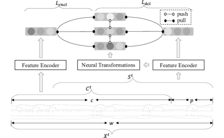
(a)

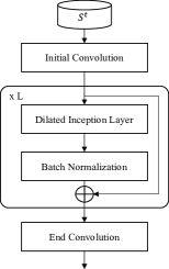
(b)

Figure 2: (a) The overall architecture of our proposed framework. (b) The inner structure of feature encoder.

4.3 Feature Encoder

The feature encoder serves the purpose of capturing temporal dependencies within a suspect or context sequence, thereby facilitating the detection of anomalies in the suspect window by identifying anomalous temporal patterns with respect to the context window. we have defined two overlapping sequences - $C^{t}$ and $S^{t}$, with equal lengths, as discussed in Section 4.1. The reason for making these sequences overlap is to ensure that their latent representations remain close to each other thus not violating our assumptions. Following the methodology employed by [3] [32], we have utilized a temporal convolution network as the base feature encoder, wherein the temporal convolution layer has been replaced by a dilated inception layer (DIL) [32] that enables the use of different kernel sizes. The general pipeline of the encoder is depicted in Figure 2(b). Note that we have demonstrated the pipeline using $S^{t}$ as input; however, the same procedure is implemented for $C^{t}$.

More specifically, we start by passing $S^{t}$ through a 1D convolution with a channel size of $d$ and a kernel size of $1$ to obtain its initial representation, $Z^{t}\in{\mathbb{R}}^{d\times c}$. Subsequently, we pass it through $L$ TCN blocks, with each containing a DIL layer followed by a batch normalization layer [12]. The residual connection is added in between each TCN blocks. After applying a sequence of TCN blocks, we obtain a final output with a dimension of $(d,1)$, which is subsequently fed through another 1D convolution layer with a kernel size of $(1,1)$ to derive the ultimate latent representation of $S^{t}$. We denote the latent representations of $S^{t}$ and $C^{t}$ as $O^{t}$ and $G^{t}$, respectively.

4.4 Optimization Framework

4.4.1 Contextual Contrastive Loss Without Regularization

Our framework assumes that normal sequences change mildly compared to abnormal sequences from recent history. To implement this, we contrast the prediction window with the context window by minimizing the distance between their hidden representations for normal samples. This approach is inspired by DeepSVDD, but allows the center of the hypersphere to vary based on the context, better adapting it to time series anomaly detection where most anomalies are contextually irregular.

Formally, let $g(\cdot,W):{\mathbb{R}}^{N\times c}\rightarrow{\mathbb{R}}^{d}$ be the feature encoder in section 4.3 with learnable weights $W$. We define a contextual contrastive loss as

$${\mathcal{L}}_{\text{ccl}}:={\mathbb{E}}_{X^{t}\sim{\mathcal{D}}}{\|g(S^{t};W)-g(C^{t};W)\|}^{2}_{2}$$ (5)

which is the mean euclidean distance between the hidden representations of the suspect sequence and context sequence. However, minimizing Eq. (5) can lead to constant encoder solutions, which we refer to as the representation collapse issue. Specifically, the optimal solution of the objective can be trivially achieved when the output of the encoder is a constant for arbitrary input values (More details in section 5).

One way to avoid the constant encoder solution is to add an objective that enforces the encoder to produce different outputs under different contexts. In this work, we explore the combination of this contextual contrastive objective with neural transformation learning [22] for time series anomaly detection.

4.4.2 Equipping With Neural Transformations

Neural transformation learning learns diverse transformations that maintain the original sample’s semantic information. We could leverage this approach to prevent the representation collapse, by contrasting the diverse but semantic-related hidden representations of the suspect feature representation $O^{t}$ against the context feature representation $G^{t}$.

Formally, given the suspect feature representation $O^{t}$, we project it into K latent representations $\{O^{t,i}\}_{i=1}^{K}$ using distinct transformation networks $T=\{T_{1},...,T_{K}|T_{k}:{\mathbb{R}}^{d}\rightarrow{\mathbb{R}}^{d}\}$. In our implementation, we choose three-layer MLPs with hidden dimension $d$ for $T_{k}$. In contrast to the original neural transformation learning, where transformations are applied to the raw inputs and fed through the feature encoder multiple times, we apply transformations directly to the hidden space to avoid computational burden. This allows us to apply the feature encoder only once, followed by K lightweight transformation encoders, reducing the overall computation required.

Concretely, to ensure the K transformations are diverse and semantically similar to the original input,  [22] proposes a discriminative contrastive loss as stated in 2.2. We rephrase it with the notation in our section

$${\mathcal{L}}_{\text{dcl}}:=-{\mathbb{E}}_{X^{t}\sim{\mathcal{D}}}\sum_{k=1}^{K}\log{\frac{h(O^{t},O^{t,k})}{h(O^{t},O^{t,k})+\sum_{l\neq k}h(O^{t,k},O^{t,l})}}$$ (6)

To adapt the neural transformation loss to our framework, we re-define a contextual neural contrastive loss $L_{\text{cncl}}$ as

$${\mathcal{L}}_{\text{cncl}}:={\mathbb{E}}_{X^{t}\sim{\mathcal{D}}}\sum_{k=1}^{K}{\|O^{t,k}-G^{t}\|}^{2}_{2}$$ (7)

where the contrastion is performed between the transformations of suspect feature representation against the context feature representation. During the training, the model architecture, including the feature encoder and the neural transformations, is optimized under a contextual discriminative contrastive loss ${\mathcal{L}}_{\text{cdcl}}$ during the training, which is defined as

$${\mathcal{L}}_{\text{cdcl}}:={\mathcal{L}}_{\text{cncl}}+{\mathcal{L}}_{\text{dcl}}$$ (8)

We prove in section 5 that the edge case, where both the outputs of the transformations and the feature encoder generates the same constant, does not minimize the joint loss in Eq. (8). Additionally, during inference, Eq. (8) can be directly utlized as an anomaly score of an input sample.

5 Theoretical Analysis

First, we prove that a constant feature encoder is an optimal solution for minimizing the contextual contrastive loss in Eq. (5).

Proposition 1

Given the feature encoder $g(\cdot;W)$ in 4.3, there exists a choice of parameters for $W$ such that the output of $g(\cdot;W)$ is always a constant, i.e., $\exists W^{*},c^{*}\ s.t.\ g(x;W^{*})=c^{*},\forall x$. In this case, $W=W^{*}$ is an optimal solution for minimizing the loss in Eq. (5).

Proof. Following the work proposed by [23], there are three settings that can lead to a constant encoder solution: 1. $W=\boldsymbol{0}$; 2. When the encoder is equipped with bias terms in some hidden layers. 3. When the encoder contains bounded activations. In all cases, the loss in Eq. (5) reaches the minimum. ∎

Next, we show that the constant encoders do not lead to the optimal solution of minimizing the contextual discriminative contrastive loss in Eq. (8).

Proposition 2

If there exists a choice of parameters for the feature encoder $g(\cdot)$ and the $K$ transformation networks $\{T_{k}(g(\cdot))\}_{k=1}^{K}$ such that ${\mathcal{L}}_{\text{cdcl}}<K\log K$, then the constant parameter setting $T_{k}(g(\cdot))=g(\cdot)=c,\forall c\in{\mathbb{R}}^{d}$ is not an optimal solution for minimizing ${\mathcal{L}}_{\text{cdcl}}$.

Proof. For simplicity, let $g_{k}(\cdot)$ denote $T_{k}(g(\cdot))$. First, note that when $g_{k}(\cdot)=g(\cdot)=c$, the contextual discriminative contrastive loss ${\mathcal{L}}_{\text{cdcl}}$ is given by $K\log K$.

Specifically, we have:

$${\mathcal{L}}_{\text{cdcl}} ={\mathcal{L}}_{\text{cncl}}+{\mathcal{L}}_{\text{dcl}}$$ (9)

$$=K\|c-c\|^{2}_{2}-K\log{\frac{c^{\prime}}{c^{\prime}+(K-1)c^{\prime}}}$$ (10)

$$=K\log K$$ (11)

where $c^{\prime}=h(c,c)$.

Assuming that there exists a parameter setting such that ${\mathcal{L}}_{\text{dcl}}<K\log K$, let $\epsilon=K\log K-{\mathcal{L}}_{\text{cdcl}}$. Since the scoring function $h(\cdot,\cdot)$ in ${\mathcal{L}}_{\text{dcl}}$ is defined as $h(g_{k}(\cdot),g(\cdot))=\exp(\frac{g_{k}(\cdot)g(\cdot)}{\tau\|g_{k}(\cdot)\|_{2}\|g(\cdot)\|_{2}})$, we can rescale the functions $\{g_{k}(\cdot)\}_{k=0}^{K}$ and $g(\cdot)$ during training such that $|g_{k}(x)|\leq\frac{\epsilon}{2K}$ and $|g(x)|\leq\frac{\epsilon}{2K}$ for all $x$. This rescaling is possible while ensuring that $h(g_{k}(x),g(x))$ remains the same, since cosine similarity between two vectors is invariant to their norms. Hence, we have:

$${\mathcal{L}}_{\text{cncl}}= {\mathbb{E}}_{X^{t}\sim{\mathcal{D}}}\sum_{k=1}^{K}\|g_{k}(O^{t})-g(G^{t})\|^{2}_{2}$$ (12)

$$\leq {\mathbb{E}}_{X^{t}\sim{\mathcal{D}}}\sum_{k=1}^{K}(\|g_{k}(O^{t})\|^{2}_{2}+\|g(G^{t})\|^{2}_{2})$$ (13)

$$< \sum_{k=1}^{K}(\frac{\epsilon}{2K}+\frac{\epsilon}{2K})=\epsilon$$ (14)

Therefore, we have ${\mathcal{L}}_{\text{cncl}}+{\mathcal{L}}_{\text{dcl}}<\epsilon+{\mathcal{L}}_{\text{dcl}}=\epsilon+K\log K-\epsilon=K\log K$. ∎

The intuition for $K\log K$ does not lead to the minimum solution of ${\mathcal{L}}_{\text{dcl}}$ is that the objective of minimizing this loss function is to make sure that the generated transformations are diverse among themselves while preserving certain semantic similarities from a given input, which contradicts the constant encoder solution. This can be easily verified empirically in our experiments.

6 Experiment

6.1 Datasets

In this work, real-world benchmark datasets are used for the evaluation of time series anomaly detection methods: SWaT [17]. WADI [1], HAI [27], SMAP and MSL [11], and SMD [28]. The statistics of data are summarized in Table 1:

Table 1: Summary statistics for datasets used in experiments

Dataset	# Channels	# training	# test	% anomalies
SWaT	51	47440	44993	12.13
WADI	123	78458	17281	5.77
SMAP	25	135183	427617	12.79
MSL	55	58317	73729	10.53
SMD	38	25300	25300	4.21
HAI	79	92163	27003	1.93
TODS	1	33333	16667	2.74

6.2 Experimental Setup and Evaluation Metric

Our model is trained with an Adam optimizer [13] at a learning rate of 0.001 for 50 epochs. $20\%$ of the training set is selected as a validation set where the best epoch is stored based on the validation loss. We employ early stopping with a patience of 10. The hidden dimension $d$ is set to 32, and the number of TCN blocks is set to 8. The temperature $\tau$ and the number of transformations for DCL loss are set to 0.1 and 6, respectively. The suspect window size $w$ is set to 5, and the sequence length is 50 for WADI, HAI, SMAP, and 30 for MSL, SWaT, SMD respectively.

F1-score is used as a performance metric to evaluate the performance of anomaly detection. The threshold for all models is chosen as the one which achieves the best F1 over the test sets. In addition, we follow the point-adjusting strategy suggested in [28], which labels a whole anomaly segment as 1 as long as one of the points within the segment is detected as an anomaly.

6.3 Baseline Methods

We compare our framework with the most commonly used baseline methods selected from two categories: 1. General deep learning-based anomaly detection algorithms: Deep SVDD [23], and DAGMM [38]. 2. Deep learning-based anomaly detection algorithms that are tailored to temporal sequences: LSTM-VAE [19], MAD-GAN [15], USAD [2], MSCRED [34], MTAD-GAT [37], GDN [6], LNT [24], and NCAD [5].

Table 2: Performance comparison (F1 (%)) on real-world datasets. The best performance is highlighted in bold.

Methods	SWaT	WADI	SMAP	MSL	HAI	SMD
DeepSVDD	82.87	67.33	69.67	85.01	44.25	86.30
DAGMM	81.83	44.34	71.05	70.07	38.27	70.94
LSTM-VAE	84.95	67.52	72.74	90.58	67.07	78.42
MAD-GAN	86.53	70.51	88.14	91.38	28.70	47.85
USAD	84.60	57.25	86.34	92.72	69.41	94.63
MSCRED	84.59	55.01	69.33	82.05	74.79	78.75
MTAD-GAT	85.50	67.94	90.13	90.84	78.91	92.72
GDN	89.57	71.54	92.31	94.62	62.54	94.84
LNT	81.31	32.63	82.65	91.82	35.61	66.00
NCAD	91.06	75.95	94.50	96.09	82.36	81.53
Ours	92.01	82.04	92.27	90.51	85.73	95.33

6.4 Comparison Study

Table 2 shows our model achieving the highest F1 scores for most datasets. However, our model’s performance falls short on MSL and SMAP. This could be due to the majority of features in these datasets being one-hot encoded commands, making temporal encoding of sequences challenging for simple TCN layers that tend to mix all features through simple sum aggregation. On the other hand, graph-based models like GDN, which explicitly learn the relationship between features, have performed well on these datasets.

Additionally, NCAD currently holds state-of-the-arts performance on MSL and SMAP due to its semi-supervised classification training schemes based on synthetic anomalies. While supervised training is known to be more effective when the underlying distribution of synthetic anomalies is similar to that of the true anomalies in the dataset, we can see that NCAD performed relatively worse in WADI, HAI, and SMD compared to our methods, suggesting potential overfitting due to these datasets having a variety of different anomaly types beyond the injected ones.

ON the other hand, LNT, a similar model to ours, showed inferior performance compared to our model, possibly because it attempts to minimize the distance between the transformation of point-wise future predictions and the context window, which may not have identical semantic meanings. In contrast, our model employs a sequence-to-sequence comparison, where the suspect and context sequences share semantically meaningful features due to their overlap and shared feature encoder.

6.5 Ablation Study

In this section, we compare different possible variants of our proposed framework against our default setting, with the details presented below:

• DCL: The feature encoder network $g(\cdot)$ is trained purely under the discriminative contrastive loss (Eq. (8)).

• CCL: The feature encoder network $g(\cdot)$ is trained purely under the contextual contrastive loss (Eq. (5)).

• OCC: The feature encoder network is trained under the one-class classification loss from DeepSVDD in a semi-supervised setting, with the training objective to map the latent representations of all normal instances into a hypersphere with minimum volume.

• CCL + reg: The encoder network $g(\cdot)$ is trained under the contextual contrastive loss, with a regularization term to enforce the variance of the latent representations of suspect and context sequences within a batch to be larger than zero. This setting is inspired by [30] [4], which is a more intuitive approach to addressing the constant encoder solution. Specifically, it is defined as:

  $${\mathcal{L}}_{\text{ccl+reg}}={\mathcal{L}}_{\text{ccl}}+v(\{S^{t}\}_{t\in B})+v(\{C^{t}\}_{t\in B})$$ (15)

  $$v(\{S^{t}\}_{t\in B})=\frac{1}{d}\sum_{j=1}^{d}\max(0,\gamma-\sqrt{\text{Var}(\{g(S^{t})_{j}\}_{t\in B})+\epsilon})$$ (16)

  where $B$ denotes an arbitrary mini-batch of samples containing $X^{t}$, $\gamma$ is set to 1 as in [4], and $\epsilon$ is a small scaler value to prevent numerical instabilities. The variance in Eq. (16) is calculated over the encoder outputs within the mini-batch $B$ during training. During inference, only ${\mathcal{L}}_{\text{ccl}}$ is used as an anomaly score for a given test instance.

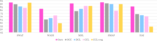
Figure 3: Performance comparison (F1 (%)) for different model variants.

Figure 3 presents the results of our experiments. The findings indicate that our model consistently outperforms the four settings. Notably, the OCC and DCL settings do not consider the contextual nature of temporally similar sequences in their loss functions, resulting in relatively poorer performance. These findings are further supported by data visualizations in subsequent sections. In contrast, the CCL setting is designed to assign similar representations to normal sequences in close proximity, but its performance falls short in comparison to our proposed approach. This can potentially be attributed to the representation collapse problem, wherein the loss function leads the encoder to converge to a parameter space that closely approximates the constant encoder solution. Consequently, the model may fail to capture the rich semantic information of normal sequences. An alternative explanation for our improved performance over CCL is that the combination of DCL and OCC losses facilitates contextual contrastion between various transformed versions of the suspect and context sequences, thereby providing diverse perspectives on the normality of the sequences and allowing the measurement of similarity between two sequences from multiple angles. This argument can be further inferred from the performance of the CCL+reg setting, wherein the addition of a variance regularization term to enforce non-constant latent representations among training samples does not outperform our default setting, and even performs worse than the CCL setting for certain datasets. In contrast, the incorporation of DCL loss in our framework not only increases the diversity of the latent representations, but also effectively forces the transformations of suspect sequences to be semantically similar to the original sequences.

6.6 Data Visualization

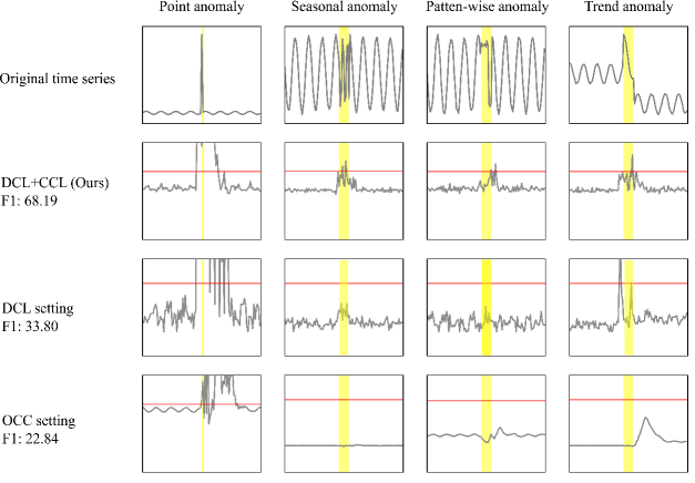
Figure 4: The above figure showcases various types of anomalies present in the TODS dataset alongside the corresponding anomaly scores generated by our proposed method, as well as the DCL and OCC settings. The red lines denote the threshold values beyond which anomalies will be identified under different settings.

To evaluate the effectiveness of our proposed framework in capturing contextual characteristics of anomalies in time series data, we conducted experiments on a univariate dataset (TODS) generated from the rules outlined in [14]. The TODS dataset adopts a sinusoidal wave as the base shapelet to generate a univariate time series, and synthetic anomalies of various types are injected using predefined rules. Examples of different types of anomalies are shown in Figure 4, and summary statistics of the data are shown in Table 1. TODS is specifically chosen for data visualization as it offers clearly classified anomalies of different types, enabling a better understanding of the performance of our model. Furthermore, the univariate nature of the dataset makes it easy to visualize the results directly from the plot.

We trained our model with three different loss functions: our default objective, the DCL setting, and the OCC setting. Figure 4 presents several showcases of different anomaly types, demonstrating the effectiveness of our proposed framework in identifying contextual anomalies. We observe that while global point anomalies are readily identifiable by all methods, OCC and DCL show relatively weaker performance in detecting other anomaly types that require contextual information. In contrast, our proposed method is capable of effectively identifying contextual anomalies by leveraging the deviation between the suspect and context window. This approach enables our method to be more sensitive to drastic changes in local context information.

7 Conclusion

In conclusion, our work introduces a novel framework for time series anomaly detection, which builds on the strengths of two popular deep anomaly detection methods, DeepSVDD and Neural AD. Our approach is supported by theoretical insights and backed by empirical results, which demonstrate that the combination of these two methods can outperform their individual usage, even when employing a simple time series sequence encoder. Additionally, our framework achieves superior performance over several widely-used baseline anomaly detection methods across multiple real-world industrial datasets.

References

- [1] Ahmed, C.M., Palleti, V.R., Mathur, A.P.: Wadi: a water distribution testbed for research in the design of secure cyber physical systems. In: Proceedings of the 3rd international workshop on cyber-physical systems for smart water networks. pp. 25–28 (2017)
- [2] Audibert, J., Michiardi, P., Guyard, F., Marti, S., Zuluaga, M.A.: Usad: Unsupervised anomaly detection on multivariate time series. In: Proceedings of the 26th ACM SIGKDD International Conference on Knowledge Discovery & Data Mining. pp. 3395–3404 (2020)
- [3] Bai, S., Kolter, J.Z., Koltun, V.: An empirical evaluation of generic convolutional and recurrent networks for sequence modeling. arXiv preprint arXiv:1803.01271 (2018)
- [4] Bardes, A., Ponce, J., LeCun, Y.: Vicreg: Variance-invariance-covariance regularization for self-supervised learning. arXiv preprint arXiv:2105.04906 (2021)
- [5] Carmona, C.U., Aubet, F.X., Flunkert, V., Gasthaus, J.: Neural contextual anomaly detection for time series. In: Raedt, L.D. (ed.) Proceedings of the Thirty-First International Joint Conference on Artificial Intelligence, IJCAI-22. pp. 2843–2851. International Joint Conferences on Artificial Intelligence Organization (7 2022). https://doi.org/10.24963/ijcai.2022/394, https://doi.org/10.24963/ijcai.2022/394, main Track
- [6] Deng, A., Hooi, B.: Graph neural network-based anomaly detection in multivariate time series. In: Proceedings of the AAAI Conference on Artificial Intelligence. vol. 35, pp. 4027–4035 (2021)
- [7] Golan, I., El-Yaniv, R.: Deep anomaly detection using geometric transformations. Advances in neural information processing systems 31 (2018)
- [8] Han, S., Woo, S.S.: Learning sparse latent graph representations for anomaly detection in multivariate time series. In: Proceedings of the 28th ACM SIGKDD Conference on Knowledge Discovery and Data Mining. pp. 2977–2986 (2022)
- [9] Hendrycks, D., Mazeika, M., Kadavath, S., Song, D.: Using self-supervised learning can improve model robustness and uncertainty. Advances in neural information processing systems 32 (2019)
- [10] Hundman, K., Constantinou, V., Laporte, C., Colwell, I., Soderstrom, T.: Detecting spacecraft anomalies using lstms and nonparametric dynamic thresholding. In: Proceedings of the 24th ACM SIGKDD international conference on knowledge discovery & data mining. pp. 387–395 (2018)
- [11] Hundman, K., Constantinou, V., Laporte, C., Colwell, I., Soderstrom, T.: Detecting spacecraft anomalies using lstms and nonparametric dynamic thresholding. In: Proceedings of the 24th ACM SIGKDD international conference on knowledge discovery & data mining. pp. 387–395 (2018)
- [12] Ioffe, S., Szegedy, C.: Batch normalization: Accelerating deep network training by reducing internal covariate shift. In: International conference on machine learning. pp. 448–456. PMLR (2015)
- [13] Kingma, D.P., Ba, J.: Adam: A method for stochastic optimization. arXiv preprint arXiv:1412.6980 (2014)
- [14] Lai, K.H., Zha, D., Xu, J., Zhao, Y., Wang, G., Hu, X.: Revisiting time series outlier detection: Definitions and benchmarks. In: Thirty-fifth conference on neural information processing systems datasets and benchmarks track (round 1) (2021)
- [15] Li, D., Chen, D., Jin, B., Shi, L., Goh, J., Ng, S.K.: Mad-gan: Multivariate anomaly detection for time series data with generative adversarial networks. In: International conference on artificial neural networks. pp. 703–716. Springer (2019)
- [16] Malhotra, P., Ramakrishnan, A., Anand, G., Vig, L., Agarwal, P., Shroff, G.: Lstm-based encoder-decoder for multi-sensor anomaly detection. arXiv preprint arXiv:1607.00148 (2016)
- [17] Mathur, A.P., Tippenhauer, N.O.: Swat: A water treatment testbed for research and training on ics security. In: 2016 international workshop on cyber-physical systems for smart water networks (CySWater). pp. 31–36. IEEE (2016)
- [18] Oord, A.v.d., Li, Y., Vinyals, O.: Representation learning with contrastive predictive coding. arXiv preprint arXiv:1807.03748 (2018)
- [19] Park, D., Hoshi, Y., Kemp, C.C.: A multimodal anomaly detector for robot-assisted feeding using an lstm-based variational autoencoder. IEEE Robotics and Automation Letters 3(3), 1544–1551 (2018)
- [20] Pranavan, T., Sim, T., Ambikapathi, A., Ramasamy, S.: Contrastive predictive coding for anomaly detection in multi-variate time series data. arXiv preprint arXiv:2202.03639 (2022)
- [21] Qiu, C., Pfrommer, T., Kloft, M., Mandt, S., Rudolph, M.: Neural transformation learning for deep anomaly detection beyond images. In: International Conference on Machine Learning. pp. 8703–8714. PMLR (2021)
- [22] Qiu, C., Pfrommer, T., Kloft, M., Mandt, S., Rudolph, M.: Neural transformation learning for deep anomaly detection beyond images. In: International Conference on Machine Learning. pp. 8703–8714. PMLR (2021)
- [23] Ruff, L., Vandermeulen, R., Goernitz, N., Deecke, L., Siddiqui, S.A., Binder, A., Müller, E., Kloft, M.: Deep one-class classification. In: International conference on machine learning. pp. 4393–4402. PMLR (2018)
- [24] Schneider, T., Qiu, C., Kloft, M., Latif, D.A., Staab, S., Mandt, S., Rudolph, M.: Detecting anomalies within time series using local neural transformations. arXiv preprint arXiv:2202.03944 (2022)
- [25] Schölkopf, B., Platt, J.C., Shawe-Taylor, J., Smola, A.J., Williamson, R.C.: Estimating the support of a high-dimensional distribution. Neural computation 13(7), 1443–1471 (2001)
- [26] Shen, L., Li, Z., Kwok, J.: Timeseries anomaly detection using temporal hierarchical one-class network. Advances in Neural Information Processing Systems 33, 13016–13026 (2020)
- [27] Shin, H.K., Lee, W., Yun, J.H., Min, B.G.: Two ics security datasets and anomaly detection contest on the hil-based augmented ics testbed. In: Cyber Security Experimentation and Test Workshop. p. 36–40. CSET ’21, Association for Computing Machinery, New York, NY, USA (2021). https://doi.org/10.1145/3474718.3474719, https://doi.org/10.1145/3474718.3474719
- [28] Su, Y., Zhao, Y., Niu, C., Liu, R., Sun, W., Pei, D.: Robust anomaly detection for multivariate time series through stochastic recurrent neural network. In: Proceedings of the 25th ACM SIGKDD international conference on knowledge discovery & data mining. pp. 2828–2837 (2019)
- [29] Tax, D.M., Duin, R.P.: Support vector data description. Machine learning 54, 45–66 (2004)
- [30] Wang, R., Liu, C., Mou, X., Guo, X., Gao, K., Liu, P., Wo, T., Liu, X.: Deep contrastive one-class time series anomaly detection. arXiv preprint arXiv:2207.01472 (2022)
- [31] Wang, S., Zeng, Y., Liu, X., Zhu, E., Yin, J., Xu, C., Kloft, M.: Effective end-to-end unsupervised outlier detection via inlier priority of discriminative network. Advances in neural information processing systems 32 (2019)
- [32] Wu, Z., Pan, S., Long, G., Jiang, J., Chang, X., Zhang, C.: Connecting the dots: Multivariate time series forecasting with graph neural networks. In: Proceedings of the 26th ACM SIGKDD international conference on knowledge discovery & data mining. pp. 753–763 (2020)
- [33] Xu, H., Wang, Y., Jian, S., Liao, Q., Wang, Y., Pang, G.: Calibrated one-class classification for unsupervised time series anomaly detection. arXiv preprint arXiv:2207.12201 (2022)
- [34] Zhang, C., Song, D., Chen, Y., Feng, X., Lumezanu, C., Cheng, W., Ni, J., Zong, B., Chen, H., Chawla, N.V.: A deep neural network for unsupervised anomaly detection and diagnosis in multivariate time series data. In: Proceedings of the AAAI conference on artificial intelligence. vol. 33, pp. 1409–1416 (2019)
- [35] Zhang, H., Cheng, F., Pandey, A.: One-class predictive autoencoder towards unsupervised anomaly detection on industrial time series (2022)
- [36] Zhang, W., Zhang, C., Tsung, F.: Grelen: Multivariate time series anomaly detection from the perspective of graph relational learning
- [37] Zhao, H., Wang, Y., Duan, J., Huang, C., Cao, D., Tong, Y., Xu, B., Bai, J., Tong, J., Zhang, Q.: Multivariate time-series anomaly detection via graph attention network. In: 2020 IEEE International Conference on Data Mining (ICDM). pp. 841–850. IEEE (2020)
- [38] Zong, B., Song, Q., Min, M.R., Cheng, W., Lumezanu, C., Cho, D., Chen, H.: Deep autoencoding gaussian mixture model for unsupervised anomaly detection. In: International conference on learning representations (2018)