We study the free and dressed propagators of physical and purely virtual particles in a finite interval of time $\tau$ and on a compact space manifold $\Omega$, using coherent states. In the free-field limit, the propagators are described by the entire function $(e^{z}-1-z)/z^{2}$, whose shape on the real axis is similar to the one of a Breit-Wigner function, with an effective width around $1/\tau$. The real part is positive, in agreement with unitarity, and remains so after including the radiative corrections, which shift the function into the physical half plane. We investigate the effects of the restriction to finite $\tau$ on the problem of unstable particles vs resonances, and show that the muon observation emerges from the right physical process, differently from what happens at $\tau=\infty$. We also study the case of purely virtual particles, and show that, if $\tau$ is small enough, there exists a situation where the geometric series of the self-energies is always convergent. The plots of the dressed propagators show testable differences: while physical particles are characterized by the usual, single peak, purely virtual particles are characterized by twin peaks.

1 Introduction

Widths are key quantities in quantum field theory, and a link between perturbative and nonperturbative quantum field theory. A perturbatively stable particle may decay after the resummation of its self-energies into the so-called dressed propagator. Yet, the resummation, which is normally considered a straightforward operation, has unexpected features, when it comes to explain the observation of long-lived unstable particles, like the muon [1].

The $S$ matrix amplitudes allow us to study scattering processes between asymptotic states, which are separated by an infinite amount of time. In this scenario, a long-lived unstable particle always has enough time to decay, before being actually observed. Although it is possible to make room for the muon observation in a rough and ready way within the usual frameworks, too many important details are missed along the way by doing so. It is much better to study the problem where it belongs, which is quantum field theory in a finite interval of time.

It is possible to formulate quantum field theory in a finite time interval $\tau$, and on a compact space manifold $\Omega$, by moving most details about such restrictions away from the internal sectors of the diagrams into external sources [2]. Then the diagrams are the same as usual, apart from the discretization of the loop momenta, and the presence of sources attached to the vertices. Most known properties of the usual $S$ matrix amplitudes generalize straightforwardly, and allow us to study the systematics of renormalization and unitarity [2]. The formulation is well-suited to be generalized so as to include purely virtual particles, i.e., particles that do not exist on the mass shell at any order of the perturbative expansion. At $\tau=\infty$, $\Omega=\mathbb{R}^{3}$, they are introduced by removing the on-shell contributions of a physical particle $\chi_{\text{ph}}$ (or a ghost $\chi_{\text{gh}}$, which is a particle with the wrong sign in front of its kinetic term) from the internal parts of the diagrams [3], and restricting to the diagrams that do not contain $\chi_{\text{ph}}$, $\chi_{\text{gh}}$ on the external legs. At finite $\tau$ and on a compact $\Omega$, they are introduced by removing the same on-shell parts from the core diagrams, and choosing trivial initial and final conditions for $\chi_{\text{ph}}$, $\chi_{\text{gh}}$ [2]. The evolution operator of the resulting theory is unitary, provided all the ghosts are rendered purely virtual.

In this paper, we study the propagators of physical and purely virtual particles in a finite interval of time $\tau$, and on a compact space manifold $\Omega$. In the free-field limit, the typical pole $1/z$ of the usual propagator at $\tau=\infty$ is replaced by an entire function, which is $f(z)=(e^{z}-1-z)/z^{2}$. Although $f(z)$ is very different from $1/z$ (and from a Breit-Wigner function) in most of the complex plane, its shape on the real axis $z=ix$, $x\in\mathbb{R}$, does remind the one of a Breit-Wigner function, with an effective width equal to $16/(3\tau)$. When we include the radiative corrections, the function $f(z)$ is shifted into the physical half plane, where the real part of the propagator remains positive, consistently with unitarity. The width is enlarged by an amount equal to $\Gamma$ (the usual width at $\tau=\infty$).

The muon observation emerges rather naturally from the right physical process: there is no need to confuse the observation of an unstable particle with the observation of its decay products, as one normally does to adjust the matter at $\tau=\infty$.

In the case of purely virtual particles, we show that, for $\tau$ small enough, there is an arrangement where the geometric series of the self-energies is always convergent. In that situation, we can resum the radiative corrections rigorously to the very end, and obtain the dressed propagator. Comparing the plot of its real part with the one of physical particles, testable differences emerge: while the physical particles are characterized by the common, single peak, purely virtual particles are characterized by two twin peaks.

The results confirm the ones of ref. [1], where they were derived by arguing, on general grounds, what the main effects of the restriction to finite $\tau$ were going to be.

Both physical particles and ghosts can be rendered purely virtual. At the same time, purely virtual particles are not Lee-Wick ghosts [4], as shown in [6]. In particular, they do not need to have nonvanishing widths, and decay. And even if they have a nonvanishing width $\Gamma_{\text{f}}$, its meaning is not the reciprocal of a lifetime, nor the actual width of a peak. In the case studied here, where the resummation of the dressed propagator can be done rigorously to the very end, $\Gamma_{\text{f}}$ is a measure of the height of the twin peaks, while their distance is universally fixed to $2\pi$ (in suitable units). In every other case, the “peak region” of a purely virtual particle is nonperturbative. Certain arguments suggest that $\Gamma_{\text{f}}$ may measure a “peak uncertainty” $\Delta E>\Gamma_{\text{f}}/2$, telling us that, when we approach the peak region too close in energy, identical experiments may give different results [1].

At the phenomenological level, purely virtual particles may have other interesting applications, because they evade many constraints that are typical of normal particles (see [7, 8, 9] and references therein).

The paper is organized as follows. In section 2 we study the free propagator at finite $\tau$. In section 3 we resum the self-energies into the dressed propagator. In section 4 we study the free and dressed propagators of purely virtual particles. In section 5 we investigate the problem of unstable particles. Section 6 contains the conclusions. We work on bosonic fields, since the generalization to fermions and gauge fields does not present problems.

2 Free propagator in a finite interval of time

In this section, we study the free propagator in a finite interval of time $\tau$. For most purposes of this paper, we can Fourier transform the space coordinates, understand the integrals on the loop momenta, and concentrate on time and energy. This means that we can basically work with quantum mechanics, where the coordinates $q(t)$ stand for fields $\phi(t,\mathbf{x})$. We assume that the Lagrangian has the form

$$L_{\lambda}(q,\dot{q})=\frac{1}{2}\left(\dot{q}^{2}-\omega^{2}q^{2}\right)-V_{\lambda}(q,\dot{q}),$$ (2.1)

where $V_{\lambda}(q)$ is proportional to some coupling $\lambda$. If the space manifold $\Omega$ is compact, the frequencies $\omega$ are restricted to a discrete set $\omega_{\mathbf{n}}$, for some label $\mathbf{n}$. This affects the propagator only in a minor way. Effects like these will be understood, from now on, so the formulas we write look practically the same as on $\Omega=\mathbb{R}^{3}$.

We use coherent “states” [10] (so we call them, although we work in the functional-integral approach)

$$z=\frac{1}{2}\left(q+i\frac{p}{\omega}\right),\qquad\bar{z}=\frac{1}{2}\left(q-i\frac{p}{\omega}\right),$$ (2.2)

where $p=\partial L_{\lambda}/\partial\dot{q}$ is the momentum. So doing, we double the number of coordinates, or fields, lower the number of time derivatives from two to one, and treat the poles of the propagator

$$\frac{i}{k^{2}-m^{2}+i\epsilon}=\frac{i}{2\omega}\left(\frac{1}{e-\omega+i\epsilon}-\frac{1}{e+\omega-i\epsilon}\right)$$ (2.3)

separately, where $k^{\mu}=(e,\mathbf{k})$ is the four-momentum and $\omega=\sqrt{\mathbf{k}^{2}+m^{2}}$ denotes the frequency.

The first pole gives the propagator

$$G^{+}(t,t^{\prime})=\langle z(t)\hskip 0.72229pt\bar{z}(t^{\prime})\rangle_{0}=\theta(t-t^{\prime})\frac{\mathrm{e}^{-i\omega(t-t^{\prime})}}{2\omega},$$ (2.4)

while the other pole gives $G^{-}(t,t^{\prime})=\langle\bar{z}(t)\hskip 0.72229ptz(t^{\prime})\rangle_{0}=G^{+}(t^{\prime},t)$. Moreover, $\langle z(t)\hskip 0.72229ptz(t^{\prime})\rangle_{0}=\langle\bar{z}(t)\hskip 0.72229pt\bar{z}(t^{\prime})\rangle_{0}=0$. The sum

$$G(t,t^{\prime})=G^{+}(t,t^{\prime})+G^{-}(t,t^{\prime})=\frac{\mathrm{e}^{-i\omega|t-t^{\prime}|}}{2\omega}$$ (2.5)

is indeed the Fourier transform of the Feynman propagator (2.3).

When $\tau=\infty$, the propagators are (2.3) and (2.4) for all real values of $t$ and $t^{\prime}$. When $\tau$ is finite, the propagators are unaffected, in the coherent-state approach, apart from the restrictions of $t$ and $t^{\prime}$ to the interval $(t_{\text{i}},t_{\text{f}})$. To make this restriction explicit, we multiply both sides of $G^{\pm}(t,t^{\prime})$ and $G(t,t^{\prime})$ by projectors $\Pi_{\tau}(t)\equiv\theta(t_{\text{f}}-t)\theta(t-t_{\text{i}})$ and $\Pi_{\tau}(t^{\prime})$. The projected propagators are then

$$G_{\tau}(t,t^{\prime})=\Pi_{\tau}(t)G(t,t^{\prime})\Pi_{\tau}(t^{\prime}),\qquad G_{\tau}^{\pm}(t,t^{\prime})=\Pi_{\tau}(t)G^{\pm}(t,t^{\prime})\Pi_{\tau}(t^{\prime}).$$ (2.6)

For simplicity, we take $t_{\text{f}}=\tau/2$, $t_{\text{i}}=-\tau/2$.

It is interesting to study the Fourier transforms of (2.6), which can be calculated by assuming that $\omega$ has a small, negative imaginary part. We start from

$$\tilde{G}_{\tau}^{+}(e,e^{\prime})=\int_{-\infty}^{+\infty}\mathrm{d}t\int_{-\infty}^{+\infty}\mathrm{d}t^{\prime}\hskip 0.72229ptG_{\tau}^{+}(t,t^{\prime})\mathrm{e}^{i(et+e^{\prime}t^{\prime})}.$$ (2.7)

Due to the lack of invariance under time translations, the result does not factorize the usual energy-conservation delta function $(2\pi)\delta(e+e^{\prime})$. Instead, we can factorize a

$$\frac{2\sin\left(\frac{e+e^{\prime}}{2}\tau\right)}{e+e^{\prime}},$$ (2.8)

which is the Fourier transform of $\Pi_{\tau}(t)$ with energy $e+e^{\prime}$. Furthermore, we assume that $\tau$ is large enough, so that we can restrict the coefficient of (2.8) in $\tilde{G}_{\tau}^{+}(e,e^{\prime})$ to $e+e^{\prime}=0$. Factorizing a $2\omega/\tau$ for convenience, we approximate $\tilde{G}_{\tau}^{+}(e,e^{\prime})$ to

$$\tilde{G}_{\tau}^{+}(e,e^{\prime})\simeq\frac{2\sin\left(\frac{e+e^{\prime}}{2}\tau\right)}{e+e^{\prime}}\frac{\tau}{2\omega}f(z),$$ (2.9)

where $z=i(e-\omega)\tau$. We find

$$f(z)=2\lim_{e^{\prime}\rightarrow-e}\frac{(e+e^{\prime})\omega\tilde{G}_{\tau}^{+}(e,e^{\prime})}{\tau\sin\left(\frac{e+e^{\prime}}{2}\tau\right)}=\frac{2\omega}{\tau^{2}}\lim_{e^{\prime}\rightarrow-e}\tilde{G}_{\tau}^{+}(e,e^{\prime})=\frac{\mathrm{e}^{z}-1-z}{z^{2}}.$$

Interestingly enough, $f(z)$ is an entire function: the propagator at finite $\tau$ has no pole, and no other type of singularity.

Writing $z=ix$, it is useful to single out the real and imaginary parts:

$$f(z)=\frac{1-\cos(x)}{x^{2}}+i\frac{x-\sin(x)}{x^{2}}.$$

To verify that the limit $\tau\rightarrow\infty$ gives the usual result, we first rescale $\tau$ by a factor $\lambda$ and then let $\lambda$ tend to infinity by means of the identities

$$\lim_{\lambda\rightarrow\infty}\frac{\sin\left(\lambda x\right)}{x}=\pi\delta(x),\qquad\lim_{\lambda\rightarrow\infty}\frac{1-\cos(\lambda x)}{\lambda x^{2}}=\pi\delta(x),\qquad\lim_{\lambda\rightarrow\infty}\frac{\lambda x-\sin(\lambda x)}{\lambda x^{2}}=\mathcal{P}\frac{1}{x}$$ (2.10)

(which can be easily proved by studying them on test functions), where $\mathcal{P}$ denotes the Cauchy principal value. Thus,

$$\lim_{\tau\rightarrow\infty}\tilde{G}_{\tau}^{+}(e,e^{\prime})=(2\pi)\delta(e+e^{\prime})\frac{1}{2\omega}\frac{i}{e-\omega+i\epsilon}=\tilde{G}^{+}(e,e^{\prime}).$$

Summing it to $\tilde{G}_{\tau}^{-}(e,e^{\prime})=\tilde{G}_{\tau}^{+}(e^{\prime},e)$, we go back to the Feynman propagator at $\tau=\infty$:

$$\tilde{G}(e,e^{\prime})=\tilde{G}^{+}(e,e^{\prime})+\tilde{G}^{-}(e,e^{\prime})=(2\pi)\delta(e+e^{\prime})\frac{i}{k^{2}-m^{2}+i\epsilon}.$$ (2.11)

Finally, the Fourier transform of the total propagator $G_{\tau}(t,t^{\prime})$ at finite $\tau$ is

$$\tilde{G}_{\tau}(e,e^{\prime})\simeq\frac{2\tau^{2}\sin\left(\frac{e+e^{\prime}}{2}\tau\right)}{e+e^{\prime}}h(x_{+},x_{-}),$$ (2.12)

where

$$h(x_{+},x_{-})\equiv\frac{f(ix_{+})+f(-ix_{-})}{x_{-}-x_{+}},\qquad x_{\pm}\equiv(e\mp\omega)\tau.$$

We see that the propagator at finite $\tau$ is encoded into the key function $f(z)$. It is convenient to compare it to a “twin” Breit-Wigner (BW) function $f_{\text{BW}}(z)$, determined so that $f(z)$ and $f_{\text{BW}}(z)$ have the same values at $z=0$ and the same $L^{2}(\mathbb{R})$ norms on the real axis (by which we mean for $z=ix$, $x\in\mathbb{R}$). We find

$$f_{\text{BW}}(z)=\frac{4}{8-3z},\qquad\lim_{z\rightarrow 0}f_{\text{BW}}(z)=\lim_{z\rightarrow 0}f(z),\qquad\int_{-\infty}^{+\infty}|f_{\text{BW}}(ix)|^{2}\mathrm{d}x=\int_{-\infty}^{+\infty}|f(ix)|^{2}\mathrm{d}x.$$ (2.13)

The width $\Gamma_{\text{eff}}$ of the twin function $f_{\text{BW}}(z)$ is a good measure of the effective width of the function $f(z)$ on the real axis. We find

$$\Gamma_{\text{eff}}=\frac{16}{3\tau},\qquad f_{\text{BW}}(i(e-\omega)\tau)=\frac{4i}{3\tau\left(e-\omega+i\frac{\Gamma_{\text{eff}}}{2}\right)}.$$ (2.14)

In fig. 1 we compare the square moduli, the real parts and the imaginary parts of $f(z)$ and $f_{\text{BW}}(z)$. We see that their slices on the real axis are similar, although the functions differ a lot in the rest of the complex plane.

It is also possible to approximate the total propagator (2.12) by replacing the function $f$ with the twin BW function $f_{\text{BW}}$. The approximation is good enough when the distance $x_{-}-x_{+}$ between the two peaks (the one of the particle and the one of the antiparticle) is large. When $x_{-}-x_{+}$ decreases, effects due to the superposition between the two peaks start to become important, although the approximation remains good qualitatively.

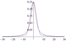
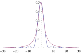
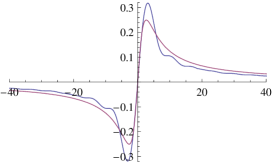
Figure 1: Comparison between $f(z)$ (in blue) and $f_{\text{BW}}(z)$ (in red): square modulus (left), real part (middle) and imaginary part (right)

Now we describe $f(z)$ for generic complex $z$. We shift $z=ix$ by a real constant $a$, with $x$ also real, and compare parallel slices $f_{a}(ix)\equiv f(ix+a)$. The typical behaviors of the real and imaginary parts of $f_{a}(ix)$ are shown in figure 2, for positive and negative $a$. We see that the real part is always positive for $a<0$, but can have both signs for $a>0$.

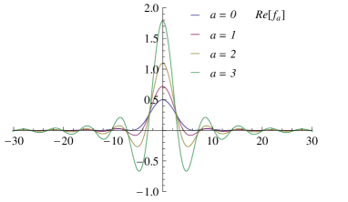
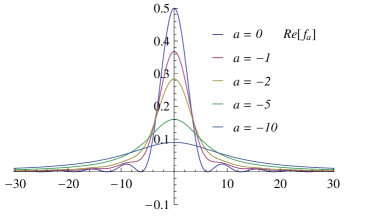
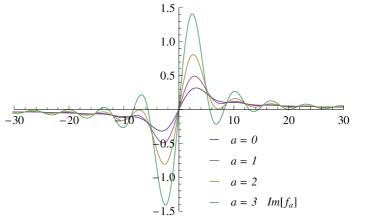
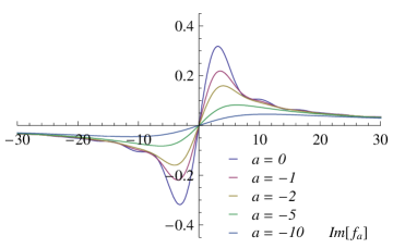
Figure 2: Real and imaginary parts of the function $f_{a}(x)=f(ix+a)$ for various values of $a$

For $a<0$, the function Re$[f_{a}(ix)]$ still looks like the real part of a BW function, but with a larger width. The physical meaning of this behavior is explained by the radiative corrections. Specifically, we show that a negative $a$ originates from the resummation of the self-energy diagrams into the dressed propagator, and is ultimately proportional to $-\Gamma$, where $\Gamma$ is the usual particle width.

3 Dressed propagator

In this section we study the dressed propagator, by resumming the corrections due to the self-energy diagrams.

Let $\Sigma(t,t^{\prime})$ denote the usual self-energy (at $\tau=\infty$) and $\Sigma_{\tau}(t,t^{\prime})$ the one at finite $\tau$. For what we are going to say, it is sufficient to focus on the one-loop corrections in the simplest case, where $-i\Sigma(t,t^{\prime})$ is the bubble diagram in coordinate space (e.g., the product of two propagators between the same, non coinciding points). Then, $\Sigma_{\tau}(t,t^{\prime})=\Pi_{\tau}(t)\Sigma(t,t^{\prime})\Pi_{\tau}(t^{\prime})$.

The dressed propagator $G_{\tau\text{d}}(t,t^{\prime})$, obtained from the mentioned resummation, reads

$$G_{\tau\text{d}}(t,t^{\prime}) = \Pi_{\tau}(t)\hat{G}_{\tau\text{d}}(t,t^{\prime})\Pi_{\tau}(t^{\prime}),$$

$$\hat{G}_{\tau\text{d}}(t,t^{\prime}) \equiv G(t,t^{\prime})+\int\mathrm{d}t_{1}\mathrm{d}t_{2}G(t,t_{1})(-i)\Sigma_{\tau}(t_{1},t_{2})G(t_{2},t^{\prime})$$ (3.1)

$$\!\!\!\!\!\!\!\!\!\!\!\!{+\int\mathrm{d}t_{1}\mathrm{d}t_{2}\mathrm{d}t_{3}\mathrm{d}t_{4}G(t,t_{1})(-i)\Sigma_{\tau}(t_{1},t_{2})G(t_{2},t_{3})(-i)\Sigma_{\tau}(t_{3},t_{4})G(t_{4},t^{\prime})+\cdots,}\qquad$$

where $\hat{G}_{\tau\text{d}}(t,t^{\prime})$ is a sort of unprojected dressed propagator.

We can work out the resummation in two ways, which are equivalent within the approximations we are making here.

In the first method we first show that $\Sigma_{\tau}$ can be replaced by $\Sigma$ inside $\hat{G}_{\tau\text{d}}(t,t^{\prime})$. This makes $\hat{G}_{\tau\text{d}}(t,t^{\prime})$ coincide with the usual dressed propagator $G_{\text{d}}(t,t^{\prime})$ at $\tau=\infty$. Then, $G_{\tau\text{d}}(t,t^{\prime})$ is the projected version of $G_{\text{d}}(t,t^{\prime})$, which can be worked out as we did in the previous section.

In Fourier transforms, the usual bubble diagram can be approximated by a constant around the peak, which encodes the mass renormalization $\Delta m^{2}$ and the (nonnegative) width $\Gamma$:

$$\Sigma(t,t^{\prime})\simeq\delta(t-t^{\prime})(\Delta m^{2}-im_{\text{ph}}\Gamma),\qquad\tilde{\Sigma}(e,e^{\prime})\simeq(2\pi)\delta(e+e^{\prime})(\Delta m^{2}-im_{\text{ph}}\Gamma),$$ (3.2)

where $m_{\text{ph}}^{2}\equiv m^{2}+\Delta m^{2}$. We ignore the radiative corrections to the normalization factor $Z$ of the propagator, since we can reinstate $Z$ at a later time. Using the approximation (3.2) as the whole self-energy, the Fourier transform of $\Sigma_{\tau}(t,t^{\prime})$ is

$$\tilde{\Sigma}_{\tau}(e,e^{\prime})\simeq\frac{2\sin\left(\frac{e+e^{\prime}}{2}\tau\right)}{e+e^{\prime}}(\Delta m^{2}-im_{\text{ph}}\Gamma).$$ (3.3)

As before, we neglect the energy nonconservation at the vertices, by assuming that $\tau$ is large enough so that we can replace the factor in front by $(2\pi)\delta(e+e^{\prime})$. We obtain $\tilde{\Sigma}_{\tau}(e,e^{\prime})\simeq\tilde{\Sigma}(e,e^{\prime})$, which means that the restriction to finite $\tau$ has negligible effects on $\hat{G}_{\tau\text{d}}(t,t^{\prime})$, and we can replace it with $G_{\text{d}}(t,t^{\prime})$. Then (3.1) gives

$$G_{\tau\text{d}}(t,t^{\prime})=\Pi_{\tau}(t)G_{\text{d}}(t,t^{\prime})\Pi_{\tau}(t^{\prime}).$$ (3.4)

Resumming the geometric series, the Fourier transform of $G_{\text{d}}(t,t^{\prime})$, which is

$$\tilde{G}_{\text{d}}(e,e^{\prime})=(2\pi)\delta(e+e^{\prime})\frac{i}{k^{2}-m_{\text{ph}}^{2}+im_{\text{ph}}\Gamma},$$ (3.5)

is the same as $\tilde{G}(e,e^{\prime})$, formula (2.11), with the replacement $m^{2}\rightarrow m_{\text{ph}}^{2}-im_{\text{ph}}\Gamma$. Then, by comparing the first formula of (2.6) with (3.4), and using (2.12), we conclude that the Fourier transform of $G_{\tau\text{d}}(t,t^{\prime})$ is

$$\tilde{G}_{\tau\text{d}}(e,e^{\prime})\simeq\left.\tilde{G}_{\tau}(e,e^{\prime})\right|_{m^{2}\rightarrow m_{\text{ph}}^{2}-im_{\text{ph}}\Gamma}=\frac{2\tau^{2}\sin\left(\frac{e+e^{\prime}}{2}\tau\right)}{e+e^{\prime}}h(x_{+\text{ph}},x_{-\text{ph}}),$$ (3.6)

where

$$\tilde{\omega}_{\text{ph}}=\sqrt{\omega_{\text{ph}}^{2}-im_{\text{ph}}\Gamma},\qquad\omega_{\text{ph}}=\sqrt{\mathbf{k}^{2}+m_{\text{ph}}^{2}},\text{\qquad}x_{\pm\text{ph}}\equiv(e\mp\tilde{\omega}_{\text{ph}})\tau.$$

We see that we just need to make the replacements

$$\pm ix_{\pm}\rightarrow\pm ix_{\pm\text{ph}}=\pm ix_{\pm}+a+ib,\qquad a+ib=i\tau\left(\omega-\tilde{\omega}_{\text{ph}}\right),$$

inside the functions $f$, with $a$, $b\in\mathbb{R}$. While $b$ is a simple translation of $x_{\pm}$, the quantity

$$a=\tau\text{Im\hskip 0.72229pt}[\tilde{\omega}_{\text{ph}}]<0$$ (3.7)

measures the displacement of the plot profile into the physical half plane. Assuming $\Gamma\ll m_{\text{ph}}$, we have $a\simeq-\tau m_{\text{ph}}\Gamma/(2\omega_{\text{ph}})$. Moreover, $a\simeq-\tau\Gamma/2$ in the static limit.

The total propagator $\tilde{G}_{\tau\text{d}}(e,e^{\prime})$ is described by the function

$$g(x,y,a)=\frac{f(i(x-y)+a)+f(-i(x+y)+a)}{2(y+ia)},\qquad y>-a>0,$$ (3.8)

where $x=(x_{+}+x_{-})/2=\tau e$, $y=(x_{-}-x_{+}-2b)/2=\omega\tau-b=\tau\hskip 0.72229pt$Re$[\tilde{\omega}_{\text{ph}}]$. The quantity $2y$ is a measure of the separation between the particle peak and the antiparticle peak. If we choose $y$ large enough, we can compare the properties of the two resummation methods more clearly, because we avoid the superposition of the two peaks. The validity of our results does not depend on this assumption.

The parameter $-a$ measures the extra width due to the radiative corrections. The inequality $y+a>0$ holds because $\tilde{\omega}_{\text{ph}}^{2}$ lies in the fourth quadrant of the complex plane, so Re$[\tilde{\omega}_{\text{ph}}]+$ Im $[\tilde{\omega}_{\text{ph}}]>0$. It is easy to check that the real part of $g(x,y,a)$ is positive, in agreement with unitarity (see fig. 3).

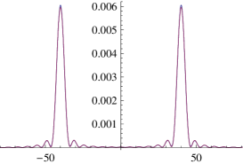
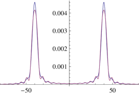
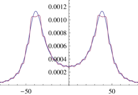
Figure 3: Plots of Re$[g(x,y,a)]$ (in blue) and Re$[g^{\prime}(x,y,a)]$ (in red) for $y=40$, $a=-1/10$ (left), $a=-1$ (middle) and $a=-10$ (right).

The second way of resumming the self-energies amounts to working directly on the Fourier transforms, by means of (2.12) and (3.3). For simplicity, we assume $\Delta m^{2}=0$ from now on, since the mass redefinition is not crucial for what we are going to say. We take care of the energy conservation by approximating the factor $(2/(e+e^{\prime}))\sin\left((e+e^{\prime})\tau/2\right)$ to $(2\pi)\delta(e+e^{\prime})$ everywhere in the sum, and switching back to the original factor only in the final formula. Then we get a straightforward geometric series, which sums to

$$\frac{(e+e^{\prime})\tilde{G}_{\tau\text{d}}^{\prime}(e,e^{\prime})}{2\tau^{2}\sin\left(\frac{e+e^{\prime}}{2}\tau\right)}\simeq h(x_{+},x_{-})\sum_{n=0}^{\infty}\left(-m\Gamma\tau^{2}h(x_{+},x_{-})\right)^{n}\equiv g^{\prime}(x,y,a).$$ (3.9)

We find

$$g^{\prime}(x,y,a)=\frac{f(i(x-\bar{y}))+f(-i(x+\bar{y}))}{2\bar{y}\left(1+\gamma f(i(x-\bar{y}))+\gamma f(-i(x+\bar{y}))\right)},$$ (3.10)

where

$$x=\tau e,\qquad\gamma=\frac{\tau m\Gamma}{2\omega}=-\frac{ay}{\bar{y}},\qquad\bar{y}=\tau\omega=\sqrt{y^{2}-a^{2}}.$$

In fig. 3 we compare Re$[g(x,y,a)]$ to Re$[g^{\prime}(x,y,a)]$ for $y=40$, $a=-1/10$, $-1$ and $-10$. We see that the approximation (3.9) captures the effects of the restriction to finite $\tau$ much better when $|a|$ is large, while the approximation (3.8) tends to smear them out. It is also easy to show that the real parts are not positive when $a$ is positive.

We can estimate the total effective width $\Gamma_{\text{tot}}$ of the dressed propagator by means of twin BW approximations, obtained by replacing $f$ with the function $f_{\text{BW}}$ of (2.13) inside (3.8) or (3.10). We assume that $y$ and $\bar{y}$ are large, to avoid superpositions between the particle and antiparticle peaks. Making the replacement $f\rightarrow$ $f_{\text{BW}}$ in $g(x,y,a)$, the shift $x\rightarrow x-ia$ in (2.14) gives

$$\Gamma_{\text{tot}}\simeq\Gamma_{\text{eff}}-\frac{2a}{\tau}=\frac{16}{3\tau}-2\text{Im\hskip 0.72229pt}[\tilde{\omega}_{\text{ph}}]\simeq\frac{16}{3\tau}+\frac{m_{\text{ph}}\Gamma}{\omega_{\text{ph}}}\simeq\frac{16}{3\tau}+\Gamma,$$ (3.11)

the last-but-one approximation being for $\Gamma\ll m_{\text{ph}}$, and the last one being at rest.

These results prove that the radiative corrections generate a shift into the physical half plane. The effective width $\Gamma_{\text{eff}}$ of the free propagator, due to the restriction to finite $\tau$, is enlarged to the total width $\Gamma_{\text{tot}}$ of the dressed propagator by an amount proportional to the usual width $\Gamma$ at $\tau=\infty$.

4 Purely virtual particles

In this section we study purely virtual particles $\chi$, taking $\Delta m^{2}=0$ again for simplicity. As recalled in the introduction, purely virtual particles are introduced by removing the on-shell contributions of ordinary particles, or ghosts, from the diagrams, perturbatively and to all orders. If we do this on the Feynman propagator (2.3), we lose $\pi\delta(k^{2}-m^{2})$ and remain with

$$\mathcal{P}\frac{i}{k^{2}-m^{2}}=\frac{i}{2\omega}\left(\mathcal{P}\frac{1}{e-\omega}-\mathcal{P}\frac{1}{e+\omega}\right).$$

where $\mathcal{P}$ denotes the Cauchy principal value. The first pole gives, after Fourier transform,

$$G_{\text{pv}}^{+}(t,t^{\prime})=\frac{\theta(t-t^{\prime})-\theta(t^{\prime}-t)}{2}\frac{\mathrm{e}^{-i\omega(t-t^{\prime})}}{2\omega}.$$

The second pole gives $G_{\text{pv}}^{-}(t,t^{\prime})=G_{\text{pv}}^{+}(t^{\prime},t)$.

The diagrams we are considering do not have $\chi$ legs inside loops (the self-energy $\Sigma$ being treated as a whole), so the $\chi$ free propagator is everything we need. Working out the Fourier transform $\tilde{G}_{\tau\hskip 0.72229pt\text{pv}}^{+}(e,e^{\prime})$ of $G_{\tau\hskip 0.72229pt\text{pv}}^{+}(t,t^{\prime})\equiv\Pi_{\tau}(t)G_{\text{pv}}^{+}(t,t^{\prime})\Pi_{\tau}(t^{\prime})$, defined as in formula (2.7), with $t_{\text{f}}=-t_{\text{i}}=\tau/2$, we find the result (2.9) with $f(z)$ replaced by

$$f_{\text{pv}}(z)=\frac{\sinh(z)-z}{z^{2}}.$$

Hence, by (2.12), the total propagator reads

$$\tilde{G}_{\tau\hskip 0.72229pt\text{pv}}(e,e^{\prime})\simeq\frac{2\tau^{2}\sin\left(\frac{e+e^{\prime}}{2}\tau\right)}{e+e^{\prime}}h_{\text{pv}}(x_{+},x_{-}),\qquad h_{\text{pv}}(x_{+},x_{-})\equiv\frac{f_{\text{pv}}(ix_{+})+f_{\text{pv}}(-ix_{-})}{x_{-}-x_{+}}.$$

The key function is now

$$f_{\text{pv}}(ix)=i\frac{x-\sin(x)}{x^{2}},$$

which satisfies the important bound

$$|f_{\text{pv}}(ix)|\leqslant\frac{1}{\pi}.$$ (4.1)

As in (3.9), the dressed propagator is a geometric series

$$\frac{(e+e^{\prime})\tilde{G}_{\tau\text{d}}^{\prime\hskip 0.72229pt\text{pv}}(e,e^{\prime})}{2\tau^{2}\sin\left(\frac{e+e^{\prime}}{2}\tau\right)}\simeq h_{\text{pv}}(x_{+},x_{-})\sum_{n=0}^{\infty}\left(-m\Gamma\tau^{2}h_{\text{pv}}(x_{+},x_{-})\right)^{n}\equiv g_{\text{pv}}^{\prime}(x,y,a),$$ (4.2)

but we cannot resum it without checking its actual convergence. The reason is that the prescription for purely virtual particles is not analytic [11, 12], so we cannot advocate analyticity to justify the continuation of the sum from its convergence domain to the rest of the complex plane, as we normally do for physical particles.

The bound (4.1) ensures that there is a situation where the series is always convergent (on the real axis). It occurs when the quantity raised to the power $n$ in the sum of (4.2) has a modulus that is always smaller than 1. In turn, this requires $\gamma=\tau m\Gamma/(2\omega)<\pi/2$, which is true for every energy $e$ and every frequency $\omega$, if $\tau\Gamma<\pi$. Thus, it is sufficient to assume

$$\Delta E\equiv\frac{\pi}{2\tau}>\frac{\Gamma}{2},$$ (4.3)

to obtain

$$g_{\text{pv}}^{\prime}(x,y,a)=\frac{f_{\text{pv}}(i(x-\bar{y}))+f_{\text{pv}}(-i(x+\bar{y}))}{2\bar{y}\left(1+\gamma f_{\text{pv}}(i(x-\bar{y}))+\gamma f_{\text{pv}}(-i(x+\bar{y}))\right)}.$$ (4.4)

When $\bar{y}$ is large, the “particle” and “antiparticle” contributions separate well enough, and we can write

$$g_{\text{pv}}^{\prime}(x,y,a)\simeq\frac{\tilde{f}_{\text{pv}}(x-\bar{y},\gamma)+\tilde{f}_{\text{pv}}(x+\bar{y},\gamma)}{2\bar{y}},\qquad\tilde{f}_{\text{pv}}(x,\gamma)=\frac{f_{\text{pv}}(ix)}{1+\gamma f_{\text{pv}}(ix)}.$$

It is easy to prove that the twin peaks of Re$[\tilde{f}_{\text{pv}}(x,\gamma)]$ occur at $x=\pm\pi$, and have Re$[\tilde{f}_{\text{pv}}(\pm\pi,\gamma)]=\gamma/(\pi^{2}+\gamma^{2})$. Thus, $\gamma$ (hence $\Gamma$) is related to the heights of the peaks, while their positions are universal. The stationary points of Re$[\tilde{f}_{\text{pv}}(x,\gamma)]$ are at $x=n\pi$, $n$ = odd, and have heights $\gamma/(n^{2}\pi^{2}+\gamma^{2})$.

In fig. 4 we compare the properties of physical and purely virtual particles through the functions Re$[g^{\prime}(x,y,a)]$ and

$$\text{Re}[g_{\text{pv}}^{\prime}(x,y,a)]=g_{\text{pv}}^{\prime\ast}(x,y,a)(m\tau^{2}\Gamma)g_{\text{pv}}^{\prime}(x,y,a),$$ (4.5)

taking $\bar{y}=30$ and $\gamma=3/2$. The right-hand side of expression (4.5) looks like the decay rate of the purely virtual particle $\chi$, because it is the product of the propagator, times (minus the real part of) the bubble diagram, times the conjugate propagator (times a further factor $\tau^{2}$, introduced for convenience). Since $\chi$ does not exist on the mass shell, the expression “decay rate” just refers to the existence of a channel mediated by it.

Fig. 4 includes the plot of the convolution

$$\int_{-\infty}^{+\infty}\mathrm{d}u\frac{4}{(4u)^{2}+\pi^{2}}\text{Re}[g_{\text{pv}}^{\prime}(x-u,y,a)]$$ (4.6)

with a Lorentzian function of width $\pi/2=\Delta x=\tau\Delta E$. The convolution is useful if we want to interpret $\Delta E$ as the resolving power of our instrumentation on the energy.

Since we are working in a finite interval of time $\tau$, we are implying that the resolving power $\Delta t$ on time itself is better than that: $\Delta t<\tau$. Then, the energy-time uncertainty relation $\Delta t\Delta E\gtrsim 1$ tells us that the uncertainty $\Delta E$ on the energy is bigger than $\sim 1/\tau$. The best situation is when that uncertainty is close to its minimum value, which is approximately equal to the $\Delta E$ defined in formula (4.3). Thus, we can view the condition (4.3) as a condition on the resolving power on the energy. If we resolve the energies too well, we cannot have enough precision in time to claim that we are working in a finite interval $\tau$. The convoluted profile of fig. 4 is probably closer to what we can see experimentally.

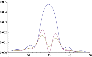
Figure 4: Comparison between the dressed propagators Re$[g^{\prime}(x,y,a)]$ and Re$[g_{\text{pv}}^{\prime}(x,y,a)]$ of physical (in blue) and purely virtual (in red and green) particles in a situation ($\gamma=3/2$) where we can trust the resummations for both. We have taken $\bar{y}=30$. The green plot is the convolution (4.6)

The plots show rather different phenomenological behaviors: while physical particles exhibit the usual peak, purely virtual particles show two smaller humps. What is important is that the difference between the two cases is experimentally testable, at least in principle.

Qualitatively, we may expect similar differences at $\tau=\infty$. However we cannot make this statement rigorous, because when $\tau$ grows we eventually violate (4.3) and enter a nonperturbative region, where we cannot trust the resummation for purely virtual particles. At the nonperturbative level, the condition (4.3) might turn into an uncertainty relation of new type [1], a “peak uncertainty” $\Delta E>\Gamma/2$, telling us that, when we approach the peak region $k^{2}\sim m^{2}$ of a purely virtual particle too closely, identical experiments may give different results.

If purely virtual particles with relatively small masses exist in nature, the predictions of this section could be tested exprimentally. Standard model extensions that are worth of attention, in this context, have been studied in refs. [7, 8]. Those models (which violate the bound (4.3), because they have $\tau=\infty$) can be used without modifications for qualitative tests. Consider, for example, processes that involve exchanges of purely virtual particles, like $Z\rightarrow\mu\mu\mu\mu$ [8]: once we reach enough precision, it should be easy to realize that the shapes of the plots are more similar to the red and green curves of fig. 4, rather than the blue curve. For quantitative tests, we need to extend the predictions of [7, 8] to a $\tau$ that is sufficiently small. The results of this paper and [2] give us the techniques we need, to achieve that goal.

More generally, the restriction to finite $\tau$, as well as the restriction to a compact space manifold $\Omega$, can be used to amplify effects that are otherwise too tiny to be observed, taking advantage of the nontrivial interplay between the observed process and the external environment (in particular, through the boundary of $\Omega$).

5 The problem of the muon (unstable particles vs resonances)

In this section we study the problem of describing the muon decay in quantum field theory. Since the muon is unstable, the right framework is not the one at $\tau=\infty$, because a too large $\tau$ gives the muon enough time to decay and, strictly speaking, makes it unobservable. If we ignore this fact and insist on describing the muon decay at $\tau=\infty$, quantum field theory retaliates by generating mathematical inconsistencies [1].

The point is that we are demanding something that violates the uncertainty principle: as stressed before, if we want to resolve a finite time (the muon lifetime in this case), we must have a finite time uncertainty $\Delta t$, which needs a nontrivial uncertainty $\Delta E$ on the energy. There are no such things in quantum field theory at $\tau=\infty$. On the other hand, a finite $\tau$ implies a finite time uncertainty $\Delta t<\tau$, so quantum field theory on a finite time interval is better equipped to address the problem we are considering. Moreover, if we want to be able to see the muon, we must have $\tau<\omega\tau_{\mu}/m_{\mu}$, where $\tau_{\mu}=1/\Gamma_{\mu}$ is the muon lifetime at rest, $m_{\mu}$ is the muon mass and $\omega/m_{\mu}$ is the boost factor, which is crucial to make the muon live longer.

Let us imagine a process where certain incoming particles $X$ collide and produce the unstable particle, or resonance, we want to study, which we denote by $\phi$. The total cross section $\sigma_{\text{tot}}$ can be split into the sum of the cross section for the production of $\phi$ itself (in which case $\phi$ does not decay during the process, and is the sole outgoing state), and the cross section for the products of the $\phi$ decay. The optical theorem tells us that $\sigma_{\text{tot}}$ is proportional to the real part of the forward scattering amplitude $X\rightarrow\phi\rightarrow X$, which receives its most important contribution around the $\phi$ peak from the $\phi$ dressed propagator. For example, we can take $X=e^{+}e^{-}$ and $\phi=Z$ to describe the $Z$ production at LEP.

The $\phi$ propagator we work with is the function

$$g^{\prime}(x,y,a)=\frac{h(x_{+},x_{-})}{1+2\gamma\bar{y}h(x_{+},x_{-})},$$ (5.1)

from formula (3.10). Its real part can be written as the sum Re$[g^{\prime}]=(\Omega_{\text{particle}}+\Omega_{\text{decay}})/\tau^{2}$ of the two terms

$$\frac{\Omega_{\text{particle}}}{\tau^{2}}=\frac{h_{1}}{|1+2\gamma\bar{y}h|^{2}},\qquad\qquad\frac{\Omega_{\text{decay}}}{\tau^{2}}=\frac{2\gamma\bar{y}|h|^{2}}{|1+2\gamma\bar{y}h|^{2}}=g^{\prime\hskip 0.72229pt\ast}(m\tau^{2}\Gamma)g^{\prime},$$ (5.2)

where $h$ stands for $h(x_{+},x_{-})$ and $h_{1}$ is its real part. The factor $1/\tau^{2}$ takes care of the analogous factor appearing on the left-hand side of (3.9). The reason behind the separation (5.2) is relatively simple to understand: $\Omega_{\text{decay}}$, which captures the $\phi$ decay, is the part proportional to the self-energy itself (i.e., proportional to $\Gamma$, in our approximation), while $\Omega_{\text{particle}}$, which captures the particle observation, is the rest. The detailed resummation of the diagrams involved in the two cases can be found in [1].

The structure of $\Omega_{\text{decay}}/\tau^{2}$ matches the one of (4.5), while the first expression has no analogue in the case of purely virtual particles (which admit no particle observation, by definition, but just a “decay” channel).

We want to study $\Omega_{\text{particle}}$ and $\Omega_{\text{decay}}$ in two limiting situations of physical interest: unstable particles and resonances.

Although we just need to take $\tau$ smaller than the boosted muon lifetime $\omega\tau_{\mu}/m_{\mu}$, it is convenient to take $\tau\ll\omega\tau_{\mu}/m_{\mu}$, both because it is realistic to do so, but also because it simplifies the results. Furthermore, in all the colliders built, or planned, so far, the muon mass $m_{\mu}$ is much larger than the resolving power on the energy, so we may assume

$$m_{\mu}\gg\frac{1}{\tau}\gg\frac{m_{\mu}}{\omega\tau_{\mu}}=\frac{m_{\mu}\Gamma_{\mu}}{\omega}.$$ (5.3)

It is easy to prove the inequality $|h(x_{+},x_{-})|\leqslant 1/(2\bar{y})$, which implies that under the assumptions (5.3), the denominator of $g^{\prime}(x,y,a)$ in (5.1) can be approximated to one, and the function $g^{\prime}(x,y,a)$ can be approximated to its free value $h(x_{+},x_{-})$ (which implies $\Omega_{\text{decay}}\rightarrow 0$).

Furthermore, the conditions (5.3) imply $\bar{y}\gg 1$. Then it is easy to prove, from the second limit of (2.10), that

$$\Omega_{\text{particle}}\simeq\pi\delta(e^{2}-\omega^{2}).$$ (5.4)

In other words, $\Omega_{\text{particle}}$ tends to the delta function that describes the muon observation, while $\Omega_{\text{decay}}$ tends to zero.

Note that we have not taken $\tau$ to infinity to prove this result. Actually, it is impossible to obtain it by working at $\tau=\infty$ [1], because in that case

$$\tau^{2}g^{\prime}(x,y,a)\rightarrow\frac{i}{e^{2}-\omega^{2}+i(\epsilon+m_{\mu}\Gamma_{\mu})},$$

which means

$$\Omega_{\text{particle}}\rightarrow\frac{\epsilon}{(e^{2}-\omega^{2})^{2}+(\epsilon+m_{\mu}\Gamma_{\mu})^{2}},\qquad\qquad\Omega_{\text{decay}}\rightarrow\frac{m_{\mu}\Gamma_{\mu}}{(e^{2}-\omega^{2})^{2}+(\epsilon+m_{\mu}\Gamma_{\mu})^{2}}.$$ (5.5)

Since $\Gamma_{\mu}$ is nonzero and $\epsilon$ is a mathematical artifact, we get $\Omega_{\text{particle}}\rightarrow 0$, while $\Omega_{\text{decay}}$ tends to the Breit-Wigner function of a resonance. Normally, people confuse $\Omega_{\text{particle}}$ and $\Omega_{\text{decay}}$, and say that, because the muon width $\Gamma_{\mu}$ is very small, one can let it tend to zero in $\left.\Omega_{\text{decay}}\right|_{\epsilon=0}$, which gives $\pi\delta(e^{2}-\omega^{2})$. However, the desired delta function should not come from $\Omega_{\text{decay}}$ (it would be like resuscitating the muon by making it eternal after its decay): it must come from $\Omega_{\text{particle}}$. This can happen only at $\tau<\infty$, as in (5.4).

In the case of a resonance, like the $Z$ boson, there is no reason why we should keep $\tau$ finite, since in all the experiments of collider physics, so far, the $Z$ lifetime $\tau_{Z}$ is much shorter than the interval $\tau$ separating the incoming particles from the outgoing ones (we are very far from observing the $Z$ boson directly):

$$m_{Z}>\Gamma_{Z}=\frac{1}{\tau_{Z}}\gg\frac{1}{\tau}.$$ (5.6)

This means that we can use the formulas (5.5) with $\mu\rightarrow Z$, where $\Omega_{\text{particle}}$ correctly gives zero, while $\Omega_{\text{decay}}$ tends to the right Breit-Wigner formula.

The processes observed in colliders fall in one of the situations just described, where the particle lifetimes $\tau_{\phi}$ are much longer, or much shorter than $\tau$. If we want to test formulas such as (5.1) beyond the approximations considered above, $\tau$ must be comparable with $\tau_{\phi}$, and the energy precisions must be comparable with the widths. We can reach the required $\tau$ with muons and tauons (a tauon with an energy equal to the maximum LHC energy, 13.6TeV, travels 66 centimeters). It is much harder to reach the required energy resolutions, because a huge gap separates the widths of the known renonances from the ones of the long-lived unstable particles: there are 19 and 12 orders of magnitude between the width of the $Z$ boson and the ones of the muon and tauon, respectively. The conclusion is that, right now, it is hard to figure out realistic intermediate situations between the two limits that we have consided. Still, it is worth to point out that, if a chance of that type ever becomes available, a way to test formulas like (5.1) is to count only particle traces with specific features, e.g., longer/shorter than some given length $\ell$ (the critical value being $\ell\sim\tau_{\phi}\bar{E}/m_{\phi}$, where $\bar{E}$ is the mean particle energy and $m_{\phi}$ is its mass). Plotting the data as functions of the muon energy, one should find a distribution with a width that is larger than $\Gamma$, as predicted by (3.11).

6 Conclusions

We have studied the propagators of physical and purely virtual particles in quantum field theory in a finite interval of time $\tau$, and on a compact manifold $\Omega$. In the free-field limit, the typical pole $1/z$ is replaced by the entire function $f(z)=(e^{z}-1-z)/z^{2}$. The shape of the latter on the real axis $z=ix$ reminds the one of a Breit-Wigner function, with an effective width equal to $16/(3\tau)$. The two functions are very different in the rest of the complex plane.

When we include the radiative corrections, the key function remains $f(z)$, but it is shifted into the physical half plane. The width is enlarged by an amount equal to $\Gamma$ (the usual width at $\tau=\infty$). The real part of the propagator is always positive, in agreement with unitarity.

We have studied the case of purely virtual particles, and showed that, for $\tau$ small enough ($\tau<\pi/\Gamma$), there is an arrangement where the geometric series of the self-energies is always convergent. The key reason is that the function $f(z)$ is bounded on the real axis and on the physical half plane. In that situation, it is possible to rigorously resum the series into the dressed propagator, and compare the result with what we find in the case of physical particles. The plots differ in ways that can in principle be tested: physical particles are characterized by the usual, single peak; instead, purely virtual particles are characterized by two twin peaks, which are separated from one another in a universal way, and have heights that depend on the width of the particle.

Finally, we have investigated the effects of the restriction to finite $\tau$ on the problem “muon vs $Z$ boson” (i.e., unstable particles vs resonances). It is crucial to work at $\tau<\infty$, if we want to properly explain the observation of an unstable particle. Once we do that, the muon observation emerges naturally from the right physical process. In particular, there is no need to confuse the observation of a particle with the observation of its decay products, and pretend that the particle resuscitates after its decay (which is basically how one normally adjusts the matter by sticking to $\tau=\infty$). The results confirm those argued in ref. [1] on general grounds.

Examples of time-dependent problems where it might be interesting to use the techniques studied here and in [2] are neutrino oscillations and kaon oscillations, as well as phenomena of the early universe and quark-gluon plasma. Hopefully, the investigation carried out here can stimulate the search for ways to overcome the paradigms that have dominated the scene in quantum field theory since its birth, by searching for purely virtual particles, on one side, and outdoing the $S$ matrix and the diagrammatics based on time ordering, on the other side. In this spirit, it may be interesting to merge the results with those of approaches like the Schwinger-Keldysh “in-in” formulation, which applies to initial value problems, and also involves a diagrammatics that is different from the standard “in-out” one.

References

- [1] D. Anselmi, Dressed propagators, fakeon self-energy and peak uncertainty, J. High Energy Phys. 06 (2022) 058, 22A1 Renorm and arXiv:2201.00832 [hep-ph].
- [2] D. Anselmi, Quantum field theory of physical and purely virtual particles in a finite interval of time on a compact space manifold: diagrams, amplitudes and unitarity, 23A1 Renorm and 2304.07642 [hep-th].
- [3] D. Anselmi, Diagrammar of physical and fake particles and spectral optical theorem, J. High Energy Phys. 11 (2021) 030, 21A5 Renorm and arXiv: 2109.06889 [hep-th].
- [4] T.D. Lee and G.C. Wick, Negative metric and the unitarity of the S-matrix, Nucl. Phys. B 9 (1969) 209; T.D. Lee and G.C. Wick, Finite theory of quantum electrodynamics, Phys. Rev. D 2 (1970) 1033. R.E. Cutkosky, P.V Landshoff, D.I. Olive, J.C. Polkinghorne, A non-analytic S matrix, Nucl. Phys. B12 (1969) 281; T.D. Lee, A relativistic complex pole model with indefinite metric, in Quanta: Essays in Theoretical Physics Dedicated to Gregor Wentzel (Chicago University Press, Chicago, 1970), p. 260. N. Nakanishi, Lorentz noninvariance of the complex-ghost relativistic field theory, Phys. Rev. D 3 (1971) 811; B. Grinstein, D. O’Connell and M.B. Wise, Causality as an emergent macroscopic phenomenon: The Lee-Wick O(N) model, Phys. Rev. D 79 (2009) 105019 and arXiv:0805.2156 [hep-th].
- [5] E. Tomboulis, 1/N expansion and renormalization in quantum gravity, Phys. Lett. B 70 (1977) 361; E. Tomboulis, Renormalizability and asymptotic freedom in quantum gravity, Phys. Lett. B 97 (1980) 77; Shapiro and L. Modesto, Superrenormalizable quantum gravity with complex ghosts, Phys. Lett. B755 (2016) 279-284 and arXiv:1512.07600 [hep-th]; L. Modesto, Super-renormalizable or finite Lee–Wick quantum gravity, Nucl. Phys. B909 (2016) 584 and arXiv:1602.02421 [hep-th]; J.F. Donoghue and G. Menezes, Unitarity, stability and loops of unstable ghosts, Phys. Rev. D 100 (2019) 105006 and arXiv:1908.02416 [hep-th].
- [6] D. Anselmi, Fakeons and Lee-Wick models, J. High Energy Phys. 02 (2018) 141, 18A1 Renorm and arXiv:1801.00915 [hep-th].
- [7] D. Anselmi, K. Kannike, C. Marzo, L. Marzola, A. Melis, K. Müürsepp, M. Piva and M. Raidal, Phenomenology of a fake inert doublet model, J. High Energy Phys. 10 (2021) 132, 21A3 Renorm and arXiv:2104.02071 [hep-ph].
- [8] D. Anselmi, K. Kannike, C. Marzo, L. Marzola, A. Melis, K. Müürsepp, M. Piva and M. Raidal, A fake doublet solution to the muon anomalous magnetic moment, Phys. Rev. D 104 (2021) 035009, 21A4 Renorm and arXiv:2104.03249 [hep-ph].
- [9] A. Melis and M. Piva, One-loop integrals for purely virtual particles, arXiv:2209.05547 [hep-ph].
- [10] J. Schwinger, The theory of quantized fields. III, Phys. Rev. 91 (1953) 728; J.R. Klauder, The action option and a Feynman quantization of spinor fields in terms of ordinary c-numbers, Ann. of Phys. (NY) 11 (1960) 123; E.C.G. Sudarshan, Equivalence of semiclassical and quantum mechanical descriptions of statistical light beams, Phys. Rev. Lett. 10 (1963) 277; R.J. Glauber, Coherent and incoherent states of the radiation field, Phys. Rev. 131 (1963) 2766.
- [11] D. Anselmi and M. Piva, A new formulation of Lee-Wick quantum field theory, J. High Energy Phys. 06 (2017) 066, 17A1 Renorm and arXiv:1703.04584 [hep-th].
- [12] D. Anselmi, On the quantum field theory of the gravitational interactions, J. High Energy Phys. 06 (2017) 086, 17A3 Renorm and arXiv: 1704.07728 [hep-th].