We provide a diagrammatic formulation of perturbative quantum field theory in a finite interval of time $\tau$, on a compact space manifold $\Omega$. We explain how to compute the evolution operator $U(t_{\text{f}},t_{\text{i}})$ between the initial time $t_{\text{i}}$ and the final time $t_{\text{f}}=t_{\text{i}}+\tau$, study unitarity and renormalizability, and show how to include purely virtual particles, by rendering some physical particles (and all the ghosts, if present) purely virtual. The details about the restriction to finite $\tau$ and compact $\Omega$ are moved away from the internal sectors of the diagrams (apart from the discretization of the three-momenta), and coded into external sources. Unitarity is studied by means of the spectral optical identities, and the diagrammatic version of the identity $U^{{\dagger}}(t_{\text{f}},t_{\text{i}})U(t_{\text{f}},t_{\text{i}})=1$. The dimensional regularization is extended to finite $\tau$ and compact $\Omega$, and used to prove, under general assumptions, that renormalizability holds whenever it holds at $\tau=\infty$, $\Omega=\mathbb{R}^{3}$. Purely virtual particles are introduced by removing the on-shell contributions of some physical particles, and the ghosts, from the core diagrams, and trivializing their initial and final conditions. The resulting evolution operator $U_{\text{ph}}(t_{\text{f}},t_{\text{i}})$ is unitary, but does not satisfy the more general identity $U_{\text{ph}}(t_{3},t_{2})U_{\text{ph}}(t_{2},t_{1})=U_{\text{ph}}(t_{3},t_{1})$. As a consequence, $U_{\text{ph}}(t_{\text{f}},t_{\text{i}})$ cannot be derived from a Hamiltonian in a standard way, in the presence of purely virtual particles.

1 Introduction

The success of perturbative quantum field theory relies on the theory of scattering, and the tests of its predictions in colliders. The $S$ matrix amplitudes describe scattering processes among “asymptotic states”, which are free, and far from the interaction region. Nevertheless, quantum field theory is much more than the $S$ matrix, and can in principle make predictions about all types of processes. For example, we can consider the effects of a scattering among particles that are still interacting. One day, we might want to build colliders to test those predictions.

While there is no conceptual difficulty in formulating quantum field theory in a finite interval of time $\tau$ and on a compact space manifold $\Omega$, and various approaches can be found in the literature, it is worth to make an effort to identify the formulation that is closer to the one we are accustomed to at $\tau=\infty$, $\Omega=\mathbb{R}^{3}$. If so, we can generalize the known properties and theorems with a minimum effort, efficiently study key principles like unitarity and renormalizability, and possibly extend to formulation to purely virtual particles [1]. It may be challenging to distinguish what is virtual from what is real, what is on the mass shell and what is not, in a finite interval of time, and on a compact manifold, so the investigation may hold intriguing surprises.

The first task is to relate as much as possible the diagrams of perturbative quantum field theory in a finite interval of time $\tau$, and on a compact space manifold $\Omega$, to the usual diagrams of the $S$ matrix amplitudes. We achieve this goal by removing (almost all) the details about the restriction to finite $\tau$ and compact $\Omega$ from the internal sectors of the diagrams, and dumping them on appropriate external sources coupled to the vertices. Only the discretization of the momenta, due to the restriction to a compact $\Omega$, enters the loop integrals. This “contamination” is the maximum allowed to generalize the study of unitarity along the lines of ref. [2], that is to say, by means of spectral optical identities, which are purely albegraic and hold threshold by threshold, for arbitrary frequencies, before integrating on the loop momenta (or summing on their discretized versions, on a compact $\Omega$). In the end, the diagrams look like ordinary Feynman diagrams, apart from the discretization of the loop momenta, and the insertion of an external source for every vertex. The usual diagrammatic properties and techniques hold unmodified, or can be extended easily.

These goals are achieved efficiently in the approach based on coherent states [3]. In every other approach they require more effort, but it is always possible to obtain equivalent results by means of a change of basis, starting from the coherent-state approach.

We consider theories with Hermitian Lagrangians. The free Hamiltonians may be bounded from below or not, depending on whether the theory contains only physical particles, or includes ghosts (particles with kinetic terms multiplied by the wrong signs). If the theory just contains physical particles, the evolution operator $U(t_{\text{f}},t_{\text{i}})$ between the initial time $t_{\text{i}}$ and the final time $t_{\text{f}}=t_{\text{i}}+\tau$ is unitary: $U^{{\dagger}}(t_{\text{f}},t_{\text{i}})U(t_{\text{f}},t_{\text{i}})=1$. If ghosts are present, an analogous identity holds (called pseudounitarity equation), but cannot be interpreted as unitarity. A theory of physical particles and ghosts also satisfies the more general identity

$$U(t_{3},t_{2})U(t_{2},t_{1})=U(t_{3},t_{1}),$$ (1.1)

for arbitrary $t_{1}$, $t_{2}$ and $t_{3}$.

We study these properties diagrammatically. Specifically, we decompose (1.1) into Cutkosky-Veltman identities [4] (see also [6]). Then, we further decompose those identities into spectral optical identities, by separating the thresholds from one another, following ref. [2]. At that point, it is relatively straightforward to turn a physical particle (or a ghost) into a purely virtual particle, when needed, by trivializing its initial and final conditions, and removing the contributions to the spectral optical identities where the particle would be on shell. This can be done according to the procedure outlined in ref. [2], or by replacing the cores of the diagrams with appropriate non time-ordered versions, as explained in ref. [1]. Interestingly enough, the physical evolution operator $U_{\text{ph}}(t_{\text{f}},t_{\text{i}})$ of a theory that contains both physical and purely virtual particles turns out to be unitary for arbitrary initial and final times: $U_{\text{ph}}^{{\dagger}}(t_{\text{f}},t_{\text{i}})U_{\text{ph}}(t_{\text{f}},t_{\text{i}})=1$. However, it does not satisfy (1.1), and cannot be derived from a Hamiltonian in a standard way.

Purely virtual particles are particles that cannot exist on the mass shell at any order of the perturbative expansion. They are not physical particles, nor ghosts, but sort of “fake” particles. It is possible to introduce them by removing all the on-shell contributions due to a physical particle or a ghost in one of the following three equivalent ways: $i$) a nonanalytic Wick rotation [7, 8], $ii$) a certain manipulation of the spectral optical identities, to remove the unwanted on-shell contributions as explained in ref. [2], and $iii$) the use of non-time-ordered diagrams, instead of the standard diagrams [1]. In all cases, the basic ingredients are two: $a$) a prescription to modify the interiors of the diagrams, and $b$) a projection to drop the unwanted particles from the external states. The final theory is unitary, provided all the ghosts are rendered purely virtual. It is important to stress that I) both physical particles and ghosts can be rendered purely virtual, and II) purely virtual particles are not [9] Lee-Wick ghosts [10], so they do not need to have nonvanishing widths, and decay. The main application of the idea is the formulation of a theory of quantum gravity [8], which provides testable predictions [12] in inflationary cosmology [13]. The diagrammatic calculations are not much more difficult than with physical particles, and it is possible to implement them in softwares like FeynCalc, FormCalc, LoopTools and Package-X [14]. At the phenomenological level, purely virtual particles open interesting possibilities, because they evade many constraints that are typical of normal particles (see [15] and references therein).

We show that, whenever a theory is renormalized at $\tau=\infty$, $\Omega=\mathbb{R}^{3}$, it is also renormalized at finite $\tau$ and on a compact space manifold $\Omega$. The counterterms are the same at the Lagrangian level, up to total derivatives (which are not renormalized). These results are not surprising, considering that the ultraviolet divergences are local, and concern the behaviors of the correlation functions at infinitesimal distances and intervals of time: renormalization should know nothing about global restrictions on $\tau$ and $\Omega$. To prove the statements just made, we first extend the analytic [16] and dimensional [17] regularization techniques to finite $\tau$ and compact $\Omega$. Then we use the extended techniques to show that everything works as expected, apart from minor changes that do not modify the final outcome.

We recall that the coherent states [3] are the eigenstates of the annihilation operator. In the functional-integral (Lagrangian) approach, the switch to coherent states simply amounts to making a change of variables from coordinates and momenta $q$, $p$ to $z\sim q+ip$, $\bar{z}\sim q-ip$ (and similarly for the fields), and setting the initial conditions on $z$, the final conditions on $\bar{z}$. For convenience, we keep referring to the new variables $z$ and $\bar{z}$ by means of the Hamiltonian terminology “coherent states” .

Ultimately, the formalism we develop in this paper gives a diagrammatic interpretation of the evolution operator $U=\mathrm{e}^{-iHt}$. As such, it is supposed to work even for the scattering of particles with long-range interactions, or if the timescale of the experiment is short enough so that the process is not well-approximated by the $S$ matrix. At the same time, it retains the perturbative character of the standard approaches to the $S$ matrix amplitudes. One has to check, on a case by case basis, whether the perturbative expansion is effectively useful, i.e., whether the radiative corrections are smaller or bigger than the contributions they are supposed to correct. It may be possible to choose the space manifold $\Omega$ in order to reduce the effective range of the interactions, and identify new situations where it makes sense to compare the experimental results with the predictions obtained by truncating the perturbative expansion to the first few orders. That said, any time it makes sense to use the evolution operator $U=\mathrm{e}^{-iHt}$ perturbatively around the free limit, the results of this paper provide a diagrammatic way to do it systematically.

The $S$ matrix amplitudes are built by switching to the interaction picture, and changing the basis to (in and out) asymptotic states, identified as residues of the propagators of the external legs, which are then amputated. This part, which is necessary to deal with the asymptotic limit, is not affected by our discussion.

It is convenient to list here the main properties of the diagrammatic rules we find, starting from those that apply to the coherent-state framework.

• The frequencies are discrete, while the energies are continuous: Fourier series are used for momenta, while Fourier transforms are used for energies.

• In theories with physical particles and possibly ghosts:

  • The cores of the diagrams are variants of the usual Feynman diagrams, where the momenta are discretized, and a suitable external source $K$ is attached to each vertex.

  • The sources $K$ and the discretization of the momenta are the sole information about the restriction to finite $\tau$ and compact $\Omega$.

  • The analytic/dimensional regularization technique can be generalized to finite $\tau$ and compact $\Omega$.

  • Once a theory is renormalized at $\tau=\infty$, $\Omega=\mathbb{R}^{3}$, it is renormalized at finite $\tau$ and compact $\Omega$, and the counterterms are the same.

  • Unitarity, pseudounitarity and the identity (1.1) can be translated diagrammatically into Cutkosky-Veltman identities, à la [4].

  • The Cutkosky-Veltman identities can be decomposed threshold by threshold into algebraic, spectral optical identities, à la [2].

• Purely virtual particles can be introduced by rendering some physical particles (and all the ghosts, if any are present) purely virtual. The features of the theories of physical and purely virtual particles are:

  • The cores of the diagrams are replaced by appropriate non time ordered diagrams.

  • Equivalently, the contributions to the spectral optical identities where the purely virtual particles would be on shell are removed.

  • No external states are associated with purely virtual particles.

  • The initial and final conditions obeyed by purely virtual particles are trivial. However, their boundary conditions (referring to the boundary of $\Omega$) need not be trivial.

  • The physical evolution operator $U_{\text{ph}}(t_{\text{f}},t_{\text{i}})$ is unitary.

  • The more general identity (1.1) does not hold.

  • It is not possible to derive $U_{\text{ph}}(t_{\text{f}},t_{\text{i}})$ from a Hamiltonian in a standard way.

In a generic approach (not based on coherent states), the propagators have additional “on-shell” contributions and infinitely many singularities. A change of basis from the coherent-state approach to an arbitrary one ensures that all the singularities mutually cancel out, and any property we prove with coherent states is general.

Although it is possible to perform the Wick rotation to Euclidean space, we always work in Minkowski spacetime, because unitarity is better studied there. The connection with finite temperature quantum field theory is not obvious, and should be worked out separately.

We mostly work in four spacetime dimensions, or in quantum mechanics, but the results hold in an arbitrary number $D$ of spacetime dimensions. When we dimensionally regularize, we understand that $D$ is a complex parameter.

Throughout the paper, we work with scalar bosons. The generalization to fermions is straightforward. In the cases of gauge theories and gravity, we can apply the techiques developed here with convenient gauge choices, such as the Feynman gauge. A more general setting (working with arbitrary gauges and arbitrary gauge-fixing parameters is useful to prove the gauge independence of physical quantities, and, in practical computations, make checks of the results) requires to overcome certain technical obstacles, which are dealt with in a separate paper [5].

We work in infinite volume $\Omega=\mathbb{R}^{3}$ till section 5, where we switch to a compact $\Omega$.

The closest approach to ours that we have found in the literature is the one of ref. [19], where the basic diagrammatics of the coherent-state approach in a finite interval of time are layed out. Beyond that, we restrict to an arbitrary compact space manifold $\Omega$, develop the systematics of regularization and renormalization, study unitarity, the identity (1.1) and the spectral optical identities diagrammatically, and extend the formulation to purely virtual particles.

The paper is organized as follows. In sections 2 and 3 we consider the approach based on position eigenstates at finite $\tau$ ($\Omega=\mathbb{R}^{3}$), and describe its main difficulties. In section 4 we switch to the approach based on coherent states, still on $\Omega=\mathbb{R}^{3}$. In section 5 we switch to a compact space manifold $\Omega$. In section 6 we generalize the analytic/dimensional regularization technique and study the renormalization of the theory. In section 7 we study unitarity, while in section 8 we work out the unitarity equations in diagrammatic form. In section 9 we extend the formulation to purely virtual particles. Section 10 contains the conclusions. In appendix A we compute some quantities needed in the paper.

2 Position-eigenstate approach

We begin by working with position eigenstates, and their field analogues, which have an intuitive interpretation. Unfortunately, they lead to unnecessary complications. For the moment, we restrict time to a finite interval $\tau$, but keep $\mathbb{R}^{3}$ as the space manifold.

2.1 Amplitudes

Let $\phi$ denote scalar bosonic fields. In the operatorial and functional-integral formulations, the transition amplitude between initial and final states $\phi_{\text{i}}(\mathbf{x})$ and $\phi_{\text{f}}(\mathbf{x})$ at times $t_{\text{i}}$ and $t_{\text{f}}$ (with $t_{\text{i}}<t_{\text{f}}$) reads

$$\langle\phi_{\text{f}},t_{\text{f}}\hskip 0.72229pt|\hskip 0.72229pt\phi_{\text{i}},t_{\text{i}}\rangle=\langle\phi_{\text{f}}\hskip 0.72229pt|\mathrm{e}^{-iH_{\lambda}\tau}|\hskip 0.72229pt\phi_{\text{i}}\rangle=\!\!\!\!\!\!\!\!\!\underset{{}_{\begin{subarray}{c}\phi(t_{\text{i}},\mathbf{x})=\phi_{\text{i}}(\mathbf{x})\\ \phi(t_{\text{f}},\mathbf{x})=\phi_{\text{f}}(\mathbf{x})\end{subarray}}}{\int}\!\!\!\!\!\!\!\!\![\mathrm{d}\phi]\exp\left(i\int_{t_{\text{i}}}^{t_{\text{f}}}\mathrm{d}t\int\mathrm{d}^{3}\mathbf{x\hskip 0.72229pt}L_{\lambda}(\phi(t,\mathbf{x}))\right),$$ (2.1)

where $\tau=t_{\text{f}}-t_{\text{i}}$, $H_{\lambda}$ is the Hamiltonian and $\mathbf{\hskip 0.72229pt}L_{\lambda}$ is the Lagrangian. We assume that $L_{\lambda}$ has the form

$$L_{\lambda}(\phi)=L_{0}(\phi)+L_{I}(\phi),\qquad L_{0}(\phi)=\frac{1}{2}(\partial_{\mu}\phi)(\partial^{\mu}\phi)-\frac{m^{2}}{2}\phi^{2},$$ (2.2)

where the interaction term $L_{I}(\phi)$ is proportional to some coupling $\lambda$, to be treated perturbatively. In various steps, it may be useful to assume, as usual, that the squared mass has a small negative imaginary part ($m^{2}\rightarrow m^{2}-i\epsilon$, $\epsilon>0$).

Let $\phi_{0}(t,\mathbf{x})$ denote the solution of the Klein-Gordon equation $\partial_{\mu}\partial^{\mu}\phi_{0}+m^{2}\phi_{0}=0$ with initial and final conditions $\phi_{0}(t_{\text{i}},\mathbf{x})=\phi_{\text{i}}(\mathbf{x})$, $\phi_{0}(t_{\text{f}},\mathbf{x})=\phi_{\text{f}}(\mathbf{x})$. We write

$$\phi(t,\mathbf{x})=\phi_{0}(t,\mathbf{x})+\varphi(t,\mathbf{x}),$$ (2.3)

so the quantum fluctuation $\varphi(t,\mathbf{x})$ has the simpler boundary conditions $\varphi(t_{\text{i}},\mathbf{x})=\varphi(t_{\text{f}},\mathbf{x})=0$. The action reads

$$S_{\lambda}(\phi)\equiv\int_{t_{\text{i}}}^{t_{\text{f}}}\!\!\mathrm{d}t\!\int\!\mathrm{d}^{3}\mathbf{x\hskip 0.72229pt\hskip 0.72229pt}L_{\lambda}(\phi(t,\mathbf{x}))=S_{\lambda}(\phi_{0})+S_{\lambda}(\varphi,\phi_{0}),\quad S_{\lambda}(\varphi,\phi_{0})\equiv\int_{t_{\text{i}}}^{t_{\text{f}}}\!\!\mathrm{d}t\!\int\!\mathrm{d}^{3}\mathbf{x\hskip 0.72229pt}L_{\lambda}(\varphi,\phi_{0}),$$ (2.4)

where

$$S_{\lambda}(\phi_{0}) = \frac{1}{2}\int\mathrm{d}^{3}\mathbf{x\hskip 0.72229pt}\left[\phi_{\text{f}}(\mathbf{x})\dot{\phi}_{0}(t_{\text{f}},\mathbf{x})-\phi_{\text{i}}(\mathbf{x})\dot{\phi}_{0}(t_{\text{i}},\mathbf{x})\right]+\int_{t_{\text{i}}}^{t_{\text{f}}}\mathrm{d}t\int\mathrm{d}^{3}\mathbf{x\hskip 0.72229pt}L_{I}(\phi_{0}),$$

$$L_{\lambda}(\varphi,\phi_{0}) \equiv L_{0}(\varphi)+L_{I}(\varphi,\phi_{0}),\qquad L_{I}(\varphi,\phi_{0})\equiv L_{I}(\phi_{0}+\varphi)-L_{I}(\phi_{0}).$$ (2.5)

Although the $\varphi$ interaction Lagrangian $L_{I}(\varphi,\phi_{0})$ may contain $\phi_{0}$-dependent terms that are linear or quadratic in $\varphi$, we treat them perturbatively, since they are proportional to $\lambda$.

For $t_{\text{i}}>t_{\text{f}}$ we define and compute the amplitudes by means of the identity

$$\langle\phi_{\text{f}},t_{\text{f}}\hskip 0.72229pt|\hskip 0.72229pt\phi_{\text{i}},t_{\text{i}}\rangle=\left(\langle\phi_{\text{f}},t_{\text{f}}\hskip 0.72229pt|\hskip 0.72229pt\phi_{\text{i}},t_{\text{i}}\rangle^{\ast}\right)^{\ast}=\langle\phi_{\text{i}},t_{\text{i}}\hskip 0.72229pt|\hskip 0.72229pt\phi_{\text{f}},t_{\text{f}}\rangle^{\ast},$$ (2.6)

where $\langle\phi_{\text{i}},t_{\text{i}}\hskip 0.72229pt|\hskip 0.72229pt\phi_{\text{f}},t_{\text{f}}\rangle$ is the same as in (2.1) with i $\leftrightarrow$ f. Note that the time ordering becomes anti-time ordering under complex conjugation. For this reason, the complex conjugation acts on $m^{2}$ as well, when the prescription $i\epsilon$ is attached to it. If the fields are not real, we have $\phi_{\text{i}}^{\ast}$ and $\phi_{\text{f}}^{\ast}$ on the right-hand side.

2.2 Correlation functions and generating functionals

As usual, it is convenient to introduce an external source $J$ coupled to the field $\phi$, by making the replacement $L_{\lambda}\rightarrow L_{\lambda}+J\phi$ in (2.1). This allows us to define the correlation functions as functional derivatives with respect to $J$. We can write

$$\langle\phi_{\text{f}},t_{\text{f}}\hskip 0.72229pt|\hskip 0.72229pt\phi_{\text{i}},t_{\text{i}}\rangle_{J}=Z_{\lambda}(J)\exp\left(iS_{\lambda}(\phi_{0})+i\int_{t_{\text{i}}}^{t_{\text{f}}}\mathrm{d}t\int\mathrm{d}^{3}\mathbf{x}\hskip 0.72229ptJ\phi_{0}\right),$$ (2.7)

where

$$Z_{\lambda}(J)=\mathrm{e}^{iW_{\lambda}(J)}\equiv\!\!\!\!\!\!\!\!\!\!\!\!\underset{\varphi(t_{\text{i}},\mathbf{x})=\varphi(t_{\text{f}},\mathbf{x})=0}{\int}\!\!\!\!\!\!\!\!\!\!\!\![\mathrm{d}\varphi]\exp\left(iS_{\lambda}(\varphi,\phi_{0})+\int_{t_{\text{i}}}^{t_{\text{f}}}\mathrm{d}t\int\mathrm{d}^{3}\mathbf{x\hskip 0.72229pt\hskip 0.72229pt}J\varphi\right).$$ (2.8)

We can reduce the effort to working out the correlation functions encoded in $Z_{\lambda}(J)$, since the factor in front of it in (2.7) is under control.

The $Z_{\lambda}$ correlation functions

$$\langle\varphi(x_{1})\cdots\varphi(x_{n})\rangle_{\lambda}=\left.Z_{\lambda}^{-1}(0)\frac{\delta^{n}Z_{\lambda}(J)}{i\delta J(x_{1})\cdots i\delta J(x_{n})}\right|_{J=0}$$ (2.9)

collect all the diagrams, including the disconnected ones and the reducible ones. Mimicking standard arguments, we can prove that $W(J)$ is the generating functional of the connected diagrams. Its Legendre transform

$$\Gamma(\Phi)=W(J)-\int_{t_{\text{i}}}^{t_{\text{f}}}\mathrm{d}t\int\mathrm{d}^{3}\mathbf{x\hskip 0.72229pt}J\Phi,\qquad\Phi=\frac{\delta W}{\delta J},$$

is the generating functional of the amputated, one-particle irreducible diagrams.

First, it is useful to show that the functional integral of a functional total derivative vanishes. That is to say, the identity

$$\!\!\!\!\!\!\!\!\!\!\!\!\underset{\varphi(t_{\text{i}},\mathbf{x})=\varphi(t_{\text{f}},\mathbf{x})=0}{\int}\!\!\!\!\!\!\!\!\!\!\!\![\mathrm{d}\varphi]\frac{\delta}{\delta\varphi(y)}\left[X(\varphi)\exp\left(iS_{\lambda}(\varphi,\phi_{0})+\int_{t_{\text{i}}}^{t_{\text{f}}}\mathrm{d}t\int\mathrm{d}^{3}\mathbf{x\hskip 0.72229pt\hskip 0.72229pt}J\varphi\right)\right]=0$$ (2.10)

holds, where $t_{\text{i}}<y^{0}<t_{\text{f}}$ and $X(\varphi)$ is a product of local functionals.

To prove (2.10), we define

$$[X]=\!\!\!\!\!\!\!\!\!\!\!\!\underset{\varphi(t_{\text{i}},\mathbf{x})=\varphi(t_{\text{f}},\mathbf{x})=0}{\int}\!\!\!\!\!\!\!\!\!\!\!\![\mathrm{d}\varphi]\hskip 0.72229ptX(\varphi)\exp\left(iS_{\lambda}(\varphi,\phi_{0})+\int_{t_{\text{i}}}^{t_{\text{f}}}\mathrm{d}t\int\mathrm{d}^{3}\mathbf{x\hskip 0.72229pt\hskip 0.72229pt}J\varphi\right)$$ (2.11)

and let $[X]_{\alpha}$ denote the same expression upon making the change of variables $\varphi(t\mathbf{,x})\rightarrow\varphi(t\mathbf{,x})+\alpha(t\mathbf{,x})$, where $\alpha(t,\mathbf{x})$ is assumed to vanish everywhere, but in a neighborhood of $y$. This assumption ensures that we can integrate the $\alpha$-dependent corrections by parts, without worrying about boundary contributions. Since $[X]_{\alpha}=[X]$, the left-hand side of (2.10) (which is the functional derivative of $[X]_{\alpha}$ with respect to $\alpha$, calculated at $\alpha=0$) must vanish.

Using (2.10), we can derive functional equations for the generating functionals. Noting that the $W$ equation is connected and the $\Gamma$ equation is irreducible, we can prove that the solutions $W$ and $\Gamma$ share the same properties. The restriction to finite $\tau$ does not pose difficulties about this. For details see, for example, [20].

2.3 Propagator

The two-point function

$$G_{\lambda}(x,y)=\langle\varphi(x)\varphi(y)\rangle_{\lambda}=\left.Z_{\lambda}^{-1}(0)\frac{\delta^{2}Z_{\lambda}(J)}{i\delta J(x)i\delta J(y)}\right|_{J=0}$$ (2.12)

defines the propagator. In the free-field limit, $G_{0}(x,y)$ is uniquely determined by the problem

$$(\square_{x}+m^{2})G_{0}(x,y) = -i\delta^{(4)}(x-y),\qquad G_{0}(y,x)=G_{0}(x,y),$$

$$G_{0}(x,y) = 0\text{ for }x^{0}=t_{\text{i}}\text{, }x^{0}=t_{\text{f}}\text{, }y^{0}=t_{\text{i}}\text{, }y^{0}=t_{\text{f}},$$ (2.13)

where $\square=\partial_{\mu}\partial^{\mu}$ and the subscript $x$ specifies that the partial derivatives are calculated with respect to $x$. The Klein-Gordon equation is derived from (2.10) with $X(\varphi)=\varphi(x)$, $\lambda=0$ and $J=0$. The second line follows from $\varphi(t_{\text{i}},\mathbf{x})=\varphi(t_{\text{f}},\mathbf{x})=0$.

At the practical level, we solve (2.13) starting from the Feynman propagator, or any other solution of the Klein-Gordon equation. Then we add the most general solution of the homogeneous equation, and determine its arbitrary coefficients from the symmetry property $G_{0}(y,x)=G_{0}(x,y)$ and the conditions that appear in the second line of (2.13). The result is reported in formula (3.5), after Fourier transforming the space coordinates.

The generating functional of the connected correlation functions in the free-field limit is

$$iW_{0}(J)=iW_{0}(0)-\int\mathrm{d}^{4}x\mathrm{\hskip 0.72229pt}\hskip 0.72229ptJ_{\bot}(x)G_{0}(x,y)J_{\bot}(y)\hskip 0.72229pt\mathrm{d}^{4}x,$$ (2.14)

where $J_{\bot}(x)=\theta(t_{\text{f}}-x^{0})\theta(x^{0}-t_{\text{i}})J(x)$. The constant $W_{0}(0)$ is worked out in appendix A. Formula $Z_{0}(J)=\mathrm{e}^{iW_{0}(J)}$ shows that the Wick theorem works as usual.

Note that there is no need to project the propagator $G_{0}$ to the interval $t_{\text{i}}<t<t_{\text{f}}$, inside the diagrams, since it is always sandwiched in between vertices or sources $J_{\bot}$, which are already projected.

2.4 Interactions

Expanding $L_{\lambda}(\varphi,\phi_{0})$ in powers of $\varphi$, we find $\phi_{0}$-dependent vertices, which can be viewed as local composite fields coupled to external sources. More explicitly, we can write

$$\int_{t_{\text{i}}}^{t_{\text{f}}}\mathrm{d}t\int\mathrm{d}^{3}\mathbf{x\hskip 0.72229pt}L_{I}(\varphi,\phi_{0})=\int\mathrm{d}^{4}x\sum_{n=1}^{\infty}\sum_{\alpha}K_{n\alpha}(x)V_{n\alpha}(\varphi(x)),$$ (2.15)

where $V_{n\alpha}(\varphi)$ is a monomial of degree $n$ in $\varphi$ and its derivatives, $\alpha$ is an extra label to distinguish the various cases, and $K_{n\alpha}(x)$ are appropriate functions, which we can interpret as external sources. They collect the projector $\theta(t_{\text{f}}-x^{0})\theta(x^{0}-t_{\text{i}})$ onto the interval $\tau$, as well as the dependence on $\phi_{0}$. The latter is encoded in the shift (5.2) of the field, which transfers directly into the generating functional $\Gamma(\Phi)$ as an identical shift of $\Phi$.

3 Quantum mechanics

To work out explicit formulas, it is convenient to Fourier transform the space coordinates, and reduce the problem to a continuum of oscillators in quantum mechanics. It is then possible to focus on a single oscillator at a time.

In this section we consider the anharmonic oscillator with Lagrangian

$$L_{\lambda}(q)=\frac{1}{2}\left(\dot{q}^{2}-\omega^{2}q^{2}\right)-V_{\lambda}(q),$$ (3.1)

where $V_{\lambda}(q)$ is proportional to some coupling $\lambda$. The amplitude we want to study is

$$\langle q_{\text{f}},t_{\text{f}}\hskip 0.72229pt|\hskip 0.72229ptq_{\text{i}},t_{\text{i}}\rangle=\langle q_{\text{f}}\hskip 0.72229pt|e^{-iH\tau}|\hskip 0.72229ptq_{\text{i}}\rangle=\!\!\!\!\!\!\!\!\!\underset{{}_{q(t_{\text{i}})=q_{\text{i}},\hskip 1.4457ptq(t_{\text{f}})=q_{\text{f}}}}{\int}\!\!\!\!\!\!\!\!\![\mathrm{d}q]\exp\left(i\int_{t_{\text{i}}}^{t_{\text{f}}}\mathrm{d}t\mathbf{\hskip 0.72229pt}L_{\lambda}(q(t))\right),$$

where $|q\rangle$ denotes the position eigenstate.

As before, we shift $q$ to $q_{0}+q$, where

$$q_{0}(t)=\frac{q_{\text{f}}\sin((t-t_{\text{i}})\omega)+q_{\text{i}}\sin((t_{\text{f}}-t)\omega)}{\sin(\omega\tau)}\qquad$$ (3.2)

is the solution of the classical equations of motion with boundary conditions $q(t_{\text{i}})=q_{\text{i}}$, $q(t_{\text{f}})=q_{\text{f}}$. After the shift, the functional integral is done on fluctuations (still called $q$) with boundary conditions $q(t_{\text{i}})=q(t_{\text{f}})=0$.

The generating functional (2.8) is

$$Z_{\lambda}(J)=\mathrm{e}^{iW_{\lambda}(J)}=\!\!\!\!\!\!\!\underset{{}_{q(t_{\text{f}})=q(t_{\text{i}})=0}}{\int}\!\!\!\!\!\!\![\mathrm{d}q]\exp\left(i\int_{t_{\text{i}}}^{t_{\text{f}}}\mathrm{d}t\int\mathrm{d}^{3}\mathbf{x\hskip 0.72229pt}\left(L_{\lambda}(q,q_{0}))+\mathbf{\hskip 0.72229pt}J(t)q(t)\right)\right),$$ (3.3)

where $L_{\lambda}(q_{0},q)=L_{0}(q)-V_{\lambda}(q_{0}+q)+V_{\lambda}(q_{0})=L_{0}(q)+\mathcal{O}(\lambda)$.

From (2.13), we see that the free two-point function $G_{0}(t,t^{\prime})=\langle q(t)q(t^{\prime})\rangle_{0}$ is the solution of the problem

$$\left(\frac{\mathrm{d}^{2}}{\mathrm{d}t^{2}}+\omega^{2}\right)G_{0}(t,t^{\prime})=-i\delta(t-t^{\prime}),\qquad G_{0}(t^{\prime},t)=G_{0}(t,t^{\prime}),\qquad G_{0}(t_{\text{i}},t^{\prime})=G_{0}(t_{\text{f}},t^{\prime})=0.$$ (3.4)

We start from the Feynman propagator $\mathrm{e}^{-i\omega|t-t^{\prime}|}/(2\omega)$, and add the (symmetrized) solutions

$$a\mathrm{e}^{i\omega(t+t^{\prime})}+b\mathrm{e}^{-i\omega(t+t^{\prime})}+c(\mathrm{e}^{i\omega(t-t^{\prime})}+\mathrm{e}^{-i\omega(t-t^{\prime})})$$

of the homogeneous equation, multiplied by arbitrary coefficients $a$, $b$, $c$. Then, we determine these constants from the boundary conditions that appear to the right of (3.4). The result is

$$G_{0}(t,t^{\prime})=i\theta(t-t^{\prime})\frac{\sin(\omega(t_{\text{f}}-t))\sin(\omega(t^{\prime}-t_{\text{i}}))}{\omega\sin(\omega\tau)}+(t\leftrightarrow t^{\prime}),$$ (3.5)

where $t_{\text{i}}<t,t^{\prime}<t_{\text{f}}$.

To check the limit $t_{\text{f}}\rightarrow+\infty$, $t_{\text{i}}\rightarrow-\infty$, we must assume, as usual, that $\omega$ has a small negative imaginary part ($\omega\rightarrow\tilde{\omega}=\omega-i\epsilon$, $\epsilon>0$). As expected, the propagator tends to the Feynman one,

$$\lim_{t_{\text{f}}\rightarrow+\infty}G_{0}(t,t^{\prime}) = \frac{\theta(t-t^{\prime})}{2\omega}\mathrm{e}^{-i\omega(t-t^{\prime})}\left(1-\mathrm{e}^{-2i\omega(t^{\prime}-t_{\text{i}})}\right)+(t\leftrightarrow t^{\prime}),$$

$$\lim_{t_{\text{i}}\rightarrow-\infty}\lim_{t_{\text{f}}\rightarrow+\infty}G_{0}(t,t^{\prime}) = \frac{1}{2\omega}\mathrm{e}^{-i\omega|t-t^{\prime}|}.$$

It is also interesting to derive the Fourier transform of (3.5), defined by extending its expression to arbitrary times $t$ and $t^{\prime}$ (instead of restricting it to the interval $t_{\text{i}}<t,t^{\prime}<t_{\text{f}}$). We find

$$\tilde{G}_{0}(e,e^{\prime})\equiv\int_{-\infty}^{+\infty}\mathrm{d}t\int_{-\infty}^{+\infty}\mathrm{d}t^{\prime}G_{0}(t,t^{\prime})\mathrm{e}^{i(et+e^{\prime}t^{\prime})}=(2\pi)\delta(e+e^{\prime})\frac{i}{e^{2}-\omega^{2}}$$

$$\quad-\frac{i\pi^{2}\mathrm{e}^{-i\omega\tau}}{\omega\sin(\omega\tau)}\left[\delta(e+e^{\prime})2\omega\delta(e^{2}-\omega^{2})-\delta(e-e^{\prime})(\mathrm{e}^{-2i\omega t_{\text{i}}}\delta(e+\omega)+\mathrm{e}^{2i\omega t_{\text{f}}}\delta(e-\omega))\right].\,\qquad$$ (3.6)

In addition to the Feynman propagator, we have two “on shell” contributions, including one proportional to $\delta(e-e^{\prime})$. The reason is that the boundary conditions break the invariance under time translations, which causes a “spontaneous” symmetry breaking of energy conservation.

When we use the propagator (3.6) inside the loop diagrams, the integrals on the loop energies are straightforward, but the integrals on the loop momenta may be challenging. The infinitely many singularities located at $\omega\tau=n\pi$, $n\in\mathbb{Z}$, cause further complications. Yet, the final result is well defined. It is not easy to prove this fact in the position-eigenstate framework, or a generic framework. Yet, it emerges quite naturally in the coherent-state approach. Once it is evident there, it extends directly to the position-eigenstate approach, as well as every other approach that can be reached from the coherent-state one by means of a change of basis.

Note that we are using Fourier transforms (3.6) in time, rather than Fourier series, because the latter make calculations much harder, and do not allow us to take advantage of the Wick rotation. It is consistent to use Fourier transforms, for the following reason. The projection onto the finite time interval $t_{\text{i}}<t<t_{\text{f}}$ acts on the quadratic part of the Lagrangian, as well as the interaction part. Inside the loop diagrams, the propagators are sandwiched in between vertices, which are projected. Moreover, we can attach projected sources $J_{\bot}$ to the external legs, as in (2.14). Provided we do this, we can ignore the projectors on the propagators. Thus, the simplest option is to extend formula (3.5) to arbitrary times $t$ and $t^{\prime}$, after which we can use the Fourier transform (3.6).

The denominator $Z_{\lambda}(0)$ of (2.9) is worked out in appendix A at $\lambda=0$.

4 Coherent-state approach

The main virtue of the coherent-state approach [3] is that it moves all the details of the restriction to finite $\tau$ outside the diagrams. The cores of the diagrams are then the same as usual, so the final results are always well defined. The key properties also survive the restriction to a compact space manifold $\Omega$, where the internal sectors of the diagrams are affected, but only in a minor way.

In this section we lay out the basic properties of the approach, starting by recalling how it works in the case of the harmonic oscillator of frequency $\omega$ and Lagrangian

$$L_{0}(q,\dot{q})=\frac{1}{2}\left(\dot{q}^{2}-\omega^{2}q^{2}\right)$$ (4.1)

at $\tau=\infty$ ($t_{\text{f}}=+\infty$, $t_{\text{i}}=-\infty$), $\Omega=\mathbb{R}^{3}$. Introducing the momentum $p=\partial L_{0}/\partial\dot{q}$, we can consider the equivalent Lagrangian

$$L_{0}^{\prime}(q,\dot{q},p,\dot{p})=\frac{1}{2}(p\dot{q}-q\dot{p}-p^{2}-\omega^{2}q^{2}).$$ (4.2)

The change of variables

$$z=\frac{1}{2}\left(q+i\frac{p}{\omega}\right),\qquad\bar{z}=\frac{1}{2}\left(q-i\frac{p}{\omega}\right),\qquad q=z+\bar{z},\qquad p=-i\omega(z-\bar{z}),$$ (4.3)

turns $L_{0}^{\prime}$ into

$$\mathcal{L}_{0}(z,\bar{z})\equiv i\omega(\bar{z}\dot{z}-\dot{\bar{z}}z)-2\omega^{2}\bar{z}z=\frac{1}{2}\eta^{\text{t}}Q\eta,$$ (4.4)

where

$$Q=2\omega\left(\begin{tabular}[]{cc}$0$&$-i\frac{\mathrm{d}}{\mathrm{d}t}-\omega$\\ $i\frac{\mathrm{d}}{\mathrm{d}t}-\omega$&$0$\end{tabular}\right),\qquad\eta=\left(\begin{tabular}[]{l}$z$\\ $\bar{z}$\end{tabular}\right).$$ (4.5)

We call the functions $z$ and $\bar{z}$ coherent “states” by analogy with the operatorial approach, even if they are just functions in the Lagrangian approach.

The free propagators are

$$\langle z(t)\hskip 0.72229pt\bar{z}(t^{\prime})\rangle_{0}=\theta(t-t^{\prime})\frac{\mathrm{e}^{-i\omega(t-t^{\prime})}}{2\omega},\qquad\langle z(t)\hskip 0.72229ptz(t^{\prime})\rangle_{0}=\langle\bar{z}(t)\hskip 0.72229pt\bar{z}(t^{\prime})\rangle_{0}=0.$$ (4.6)

When we include the interactions, the momentum $p$ and the Hamiltonian $H_{\lambda}(p,q)$, which are

$$p=\frac{\partial L_{\lambda}}{\partial\dot{q}},\qquad H_{\lambda}(p,q)=p\dot{q}-L_{\lambda}(q,\dot{q})=H_{0}(p,q)+H_{I}(p,q),$$

allow us to replace (3.1) with

$$L_{\lambda}^{\prime}(q,\dot{q},p,\dot{p})=\frac{1}{2}(p\dot{q}-q\dot{p})-H_{\lambda}(p,q).$$ (4.7)

As before, we assume that the interaction term $H_{I}(p,q)$ is proportional to some coupling $\lambda$.

Expressing $p$ and $q$ as in (4.3), we obtain the interaction Lagrangian $\mathcal{L}_{I}(z,\bar{z})=-H_{I}(p,q)$, which does not depend on the time derivatives of $z$ and $\bar{z}$. The total Lagrangian is thus

$$\mathcal{L}_{\lambda}(z,\bar{z})=\mathcal{L}_{0}(z,\bar{z})+\mathcal{L}_{I}(z,\bar{z}).$$ (4.8)

For various purposes, it may be convenient to switch back and forth between the variables $p$, $q$ and $z$, $\bar{z}$. For example, when we upgrade from quantum mechanics to quantum field theory, (4.2) is local, while (4.8) may contain spurious nonlocalities due to the dependence of $\omega$ on the momentum.

Note that the propagator of $z+\bar{z}$ is the usual Feynman one,

$$\langle[z(t)+\bar{z}(t)]\hskip 0.72229pt[z(t^{\prime})+\bar{z}(t^{\prime})]\rangle_{0}=\frac{\mathrm{e}^{-i\omega|t-t^{\prime}|}}{2\omega}=\int\frac{\mathrm{d}e}{2\pi}\int\frac{\mathrm{d}e^{\prime}}{2\pi}\frac{i(2\pi)\delta(e+e^{\prime})\mathrm{e}^{-i(et+e^{\prime}t^{\prime})}}{e^{2}-\omega^{2}+i\epsilon}.$$ (4.9)

It is convenient to couple $z$ and $\bar{z}$ to independent sources $\bar{\zeta}$ and $\zeta$ and write the functional integral as

$$Z(\zeta,\bar{\zeta})=\int[\mathrm{d}z\mathrm{d}\bar{z}]\mathrm{\exp}\left(\int_{t_{\text{i}}}^{t_{\text{f}}}\mathrm{d}t\hskip 0.72229pt\mathcal{L}_{\lambda}(z,\bar{z})+i\int(\bar{\zeta}z+\bar{z}\zeta)\mathrm{d}t\right).$$

The reason is that the change of variables (4.3) amounts to lowering the number of time derivatives of the kinetic terms from two to one, and doubling the number of propagating independent fields: from $q$ only to $z$ and $\bar{z}$ (or $q$ and $p$). This way, the particle and antiparticle poles $e=\pm\omega$ in (4.9) are assigned to different fields. Doubling the sources as well, we can distinguish the poles $e=\pm\omega$ on the external legs of the diagrams.

4.1 Finite time interval

When we restrict to a finite time interval $\tau=t_{\text{f}}-t_{\text{i}}$, the action becomes

$$S_{\lambda}(z,\bar{z})=-i\omega\left(\bar{z}_{\text{f}}z(t_{\text{f}})+\bar{z}(t_{\text{i}})z_{\text{i}}\right)+\int_{t_{\text{i}}}^{t_{\text{f}}}\mathrm{d}t\hskip 0.72229pt\mathcal{L}_{\lambda}(z,\bar{z}),$$ (4.10)

with initial and final conditions $z(t_{\text{i}})=z_{\text{i}}$, $\bar{z}(t_{\text{f}})=\bar{z}_{\text{f}}$, where $\mathcal{L}_{\lambda}(z,\bar{z})$ is given by (4.8). The corrections to the integral of $\mathcal{L}_{\lambda}$ that appear on the right-hand side must be included in order to have the right classical variational problem. Indeed, the variation of those corrections compensates the contributions due to the total derivative contained in the expression

$$\delta\mathcal{L}_{0}(z,\bar{z})=i\omega\frac{\mathrm{d}}{\mathrm{d}t}(\bar{z}\delta z-z\delta\bar{z})+2i\omega\delta\bar{z}(\dot{z}+i\omega z)-2i\omega(\dot{\bar{z}}-i\omega\bar{z})\delta z,$$

where $\delta z$ and $\delta\bar{z}$ denote the variations of $z$ and $\bar{z}$. The cancellation just mentioned is crucial: without it, the variational problem gives the extra conditions $\bar{z}_{\text{f}}=z_{\text{i}}=0$, which trivialize the set of solutions of the classical equations of motion. Note that the interaction Lagrangian $\mathcal{L}_{I}(z,\bar{z})$ does not generate total derivatives, since it does not depend on $\dot{z}$ and $\dot{\bar{z}}$.

Introducing the sources $\zeta$ and $\bar{\zeta}$, the transition amplitude is

$$\langle\bar{z}_{\text{f}},t_{\text{f}};z_{\text{i}},t_{\text{i}}\rangle_{\zeta,\bar{\zeta}}=\!\!\!\!\!\!\!\!\!\!\!\!\!\underset{z(t_{\text{i}})=z_{\text{i}},\,\bar{z}(t_{\text{f}})=\bar{z}_{\text{f}}}{\int}\!\!\!\!\!\!\!\!\!\!\!\![\mathrm{d}z\mathrm{d}\bar{z}]\mathrm{\exp}\left(iS_{\lambda}(z,\bar{z})+\int_{t_{\text{i}}}^{t_{\text{f}}}\mathrm{d}t\hskip 0.72229pt(\bar{\zeta}z+\bar{z}\zeta)\right).$$ (4.11)

By means of the change of variables

$$z(t)=z_{0}(t)+w(t),\qquad\bar{z}(t)=\bar{z}_{0}(t)+\bar{w}(t),$$ (4.12)

we shift the trajectories $z(t)$, $\bar{z}(t)$ by the solutions

$$z_{0}(t)=z_{\text{i}}\mathrm{e}^{-i\omega(t-t_{\text{i}})},\qquad\bar{z}_{0}(t)=z_{\text{f}}\mathrm{e}^{-i\omega(t_{\text{f}}-t)},$$ (4.13)

of the classical problem at $\lambda=0$, which is

$$\left(i\frac{\mathrm{d}}{\mathrm{d}t}-\omega\right)z_{0}(t)=0,\qquad z_{0}(t_{\text{i}})=z_{\text{i}},\qquad\left(-i\frac{\mathrm{d}}{\mathrm{d}t}-\omega\right)\bar{z}_{0}(t)=0,\qquad\bar{z}_{0}(t_{\text{f}})=\bar{z}_{\text{f}}.$$

Then the fluctuations $w(t)$, $\bar{w}(t)$ are integrated with the simpler conditions $w(t_{\text{i}})=0$, $\bar{w}(t_{\text{f}})=0$.

The functional integral (4.11) turns into

$$\langle\bar{z}_{\text{f}},t_{\text{f}};z_{\text{i}},t_{\text{i}}\rangle_{\zeta,\bar{\zeta}}=\exp\left(iS_{\lambda}(z_{0},\bar{z}_{0})+\int_{t_{\text{i}}}^{t_{\text{f}}}\mathrm{d}t\hskip 0.72229pt\left(\bar{\zeta}z_{0}+\bar{z}_{0}\zeta\right)\right)Z_{\lambda}(\zeta,\bar{\zeta}),$$ (4.14)

where

$$S_{\lambda}(z_{0},\bar{z}_{0}) = -2i\omega\bar{z}_{\text{f}}\mathrm{e}^{-i\omega\tau}z_{\text{i}}+\int_{t_{\text{i}}}^{t_{\text{f}}}\mathrm{d}t\hskip 0.72229pt\mathcal{L}_{I}(z_{0},\bar{z}_{0}),$$

$$Z_{\lambda}(\zeta,\bar{\zeta})=\mathrm{e}^{iW_{\lambda}(\zeta,\bar{\zeta})}=\!\!\!\!\!\!\!\!\!\!\!\! \underset{w(t_{\text{i}})=\bar{w}(t_{\text{f}})=0}{\int}\!\!\!\!\!\!\!\!\!\![\mathrm{d}w\mathrm{d}\bar{w}]\mathrm{\exp}\left(iS_{\lambda}(w,\bar{w},z_{0},\bar{z}_{0})+\int_{t_{\text{i}}}^{t_{\text{f}}}\mathrm{d}t\hskip 0.72229pt\left(\bar{\zeta}w+\bar{w}\zeta\right)\right),\quad$$ (4.15)

while the action $S_{\lambda}$ of the fluctuations $w$ and $\bar{w}$, and its Lagrangian are

$$S_{\lambda}(w,\bar{w},z_{0},\bar{z}_{0}) = \int_{t_{\text{i}}}^{t_{\text{f}}}\mathrm{d}t\hskip 0.72229pt\mathcal{L}_{\lambda}(w,\bar{w},z_{0},\bar{z}_{0}),$$

$$\mathcal{L}_{\lambda}(w,\bar{w},z_{0},\bar{z}_{0}) = \mathcal{L}_{0}(w,\bar{w})+\mathcal{L}_{I}(z_{0}+w,\bar{z}_{0}+\bar{w})-\mathcal{L}_{I}(z_{0},\bar{z}_{0}).$$ (4.16)

As in (2.10), the functional integral of a functional total derivative vanishes:

$$\!\!\!\!\!\!\!\!\!\underset{w(t_{\text{i}})=\bar{w}(t_{\text{f}})=0}{\int}\!\!\!\!\!\!\!\!\![\mathrm{d}w\mathrm{d}\bar{w}]\frac{\delta}{\delta\tilde{w}(t^{\prime})}\left[X(w,\bar{w})\exp\left(iS_{\lambda}(w,\bar{w},z_{0},\bar{z}_{0})+\int_{t_{\text{i}}}^{t_{\text{f}}}\mathrm{d}t\mathbf{\hskip 0.72229pt}\left(\bar{\zeta}w+\bar{w}\zeta\right)\right)\right]=0,$$ (4.17)

where $t_{\text{i}}<t^{\prime}<t_{\text{f}}$, $\tilde{w}$ can stand for $w$ or $\bar{w}$, and $X(w,\bar{w})$ is a product of local functionals. Standard arguments show that $W(\zeta,\bar{\zeta})$ is the generating functional of the connected diagrams, and its Legendre transform $\Gamma$ is the generating functional of the amputated, one-particle irreducible diagrams.

To study $Z_{\lambda}(\zeta,\bar{\zeta})$ and $W_{\lambda}(\zeta,\bar{\zeta})$, it is sufficient to consider the diagrams of $w$ and $\bar{w}$. We start from the free theory

$$Z_{0}(\zeta,\bar{\zeta})=\exp\left(iW_{0}(\zeta,\bar{\zeta})\right)=\!\!\!\!\!\!\!\!\!\!\!\!\underset{w(t_{\text{i}})=\bar{w}(t_{\text{f}})=0}{\int}\!\!\!\!\!\!\!\!\!\![\mathrm{d}w\mathrm{d}\bar{w}]\mathrm{\exp}\left(i\int_{t_{\text{i}}}^{t_{\text{f}}}\mathrm{d}t\hskip 0.72229pt\left(\mathcal{L}_{0}(w,\bar{w})+\bar{\zeta}w+\bar{w}\zeta\right)\right).$$

The key property of the coherent-state approach is that the free propagators of the quantum fluctuations $w$, $\bar{w}$ coincide with those of $z$, $\bar{z}$ at $\tau=\infty$, given in formula (4.6):

$$\langle w(t)\hskip 0.72229pt\bar{w}(t^{\prime})\rangle_{0}=\theta(t-t^{\prime})\frac{\mathrm{e}^{-i\omega(t-t^{\prime})}}{2\omega},\qquad\langle w(t)\hskip 0.72229ptw(t^{\prime})\rangle_{0}=\langle\bar{w}(t)\hskip 0.72229pt\bar{w}(t^{\prime})\rangle_{0}=0.$$ (4.18)

Indeed, they can be worked out by solving the same equations (which follow from (4.17) with $X(w,\bar{w})=w$ or $\bar{w}$), with the initial and final conditions $w(t_{\text{i}})=\bar{w}(t_{\text{f}})=0$. The theta functions in (4.18) ensure that the solutions do not depend on $t_{\text{i}}$ and $t_{\text{f}}$, so the propagators at $\tau=\infty$ and $\tau<\infty$ are exactly the same.

In other words, in the coherent-state approach the propagators know nothing about $t_{\text{f}}$ and $t_{\text{i}}$, and all the features due the restriction to finite $\tau$ can be removed from the internal sectors of the diagrams, and dumped on the external sectors. In the approach based on position eigenstates, instead, the propagators include on-shell corrections that depend on $t_{\text{f}}$ and $t_{\text{i}}$ in a complicated way, as shown by formulas (3.6).

We have

$$iW_{0}(\zeta,\bar{\zeta})=-\frac{i\omega\tau}{2}-\int_{t_{\text{i}}}^{t_{\text{f}}}\mathrm{d}t\int_{t_{\text{i}}}^{t_{\text{f}}}\mathrm{d}t^{\prime}\hskip 0.72229pt\bar{\zeta}(t)\theta(t-t^{\prime})\frac{\mathrm{e}^{-i\omega(t-t^{\prime})}}{2\omega}\zeta(t^{\prime}),$$ (4.19)

where $W_{0}(0,0)=-\omega\tau/2$ is calculated in appendix A.

Now we explain how to treat the vertices. From (4.16) we see that, expanding $\mathcal{L}_{I}(z_{0}+w,\bar{z}_{0}+\bar{w})-\mathcal{L}_{I}(z_{0},\bar{z}_{0})$ in powers of $w$ and $\bar{w}$, the vertices have the form

$$V_{n,\bar{n},n^{\prime},\bar{n}^{\prime}}=\int_{t_{\text{i}}}^{t_{\text{f}}}\mathrm{d}t\hskip 0.72229ptw^{n}(t)\bar{w}^{\bar{n}}(t)\dot{w}^{n^{\prime}}(t)\dot{\bar{w}}^{\bar{n}^{\prime}}(t)f_{V}(t)=\int_{-\infty}^{+\infty}\mathrm{d}t\hskip 0.72229ptw^{n}(t)\bar{w}^{\bar{n}}(t)\dot{w}^{n^{\prime}}(t)\dot{\bar{w}}^{\bar{n}^{\prime}}(t)F_{V}(t),$$

where $f_{V}(t)$ is a certain function built with the solutions $z_{0}$ and $\bar{z}_{0}$, while $F_{V}(t)=f_{V}(t)\theta(t_{\text{f}}-t)\theta(t-t_{\text{i}})$. Performing the Fourier transform, we obtain

$$V_{n,\bar{n},n^{\prime},\bar{n}^{\prime}}=\int_{-\infty}^{+\infty}\left(\prod_{i=1}^{N}\frac{\mathrm{d}e_{i}}{2\pi}\tilde{w}_{i}(e_{i})\right)\hskip 0.72229ptK(-E),\qquad N=n+\bar{n}+n^{\prime}+\bar{n}^{\prime},\qquad E=\sum_{i=1}^{N}e_{i},$$

where $\tilde{w}_{i}\hskip 0.72229pt$ denotes the Fourier transform of $w$, $\bar{w}$, $\dot{w}$ or $\dot{\bar{w}}$, depending on the case, and $K(e)$ is the Fourier transform of $F_{V}(t)$. We obtain an ordinary vertex coupled to an external source $K$. To emphasize this fact, we write the interaction Lagrangian as

$$\int_{t_{\text{i}}}^{t_{\text{f}}}\mathrm{d}t\left(\mathcal{L}_{I}(z_{0}+w,\bar{z}_{0}+\bar{w})-\mathcal{L}_{I}(z_{0},\bar{z}_{0})\right)\equiv\int_{-\infty}^{+\infty}\mathrm{d}t\mathcal{L}_{IK}^{w}(w,\bar{w},K),$$

where $\mathcal{L}_{IK}^{w}$ collects the vertices coupled to the sources $K$. From now on, we understand that the integration limits of the integrals are $\pm\infty$, when they are not specified.

We can write

$$\exp\left(iW_{\lambda}(\zeta,\bar{\zeta})\right)=\mathrm{\exp}\left(i\int\mathrm{d}t\mathcal{L}_{IK}^{w}\left(\frac{\delta}{i\delta\bar{\zeta}}+\frac{\delta}{i\delta\zeta},K\right)\right)\exp\left(iW_{0}(\zeta,\bar{\zeta})\right).$$ (4.20)

Since the vertices of $\mathcal{L}_{IK}^{w}$ are projected to the interval $t_{\text{i}}\leqslant t\leqslant t_{\text{f}}$, it may be convenient to extend the propagators to arbitrary times as explained before. To do so, we replace $W_{0}(\zeta,\bar{\zeta})$ with

$$\tilde{W}_{0}(\zeta,\bar{\zeta})=-\frac{i\omega\tau}{2}-\int\mathrm{d}t\int\mathrm{d}t^{\prime}\hskip 0.72229pt\bar{\zeta}(t)\theta(t-t^{\prime})\frac{\mathrm{e}^{-i\omega(t-t^{\prime})}}{2\omega}\zeta(t^{\prime})$$

and define

$$\exp\left(i\tilde{W}_{\lambda}(\zeta,\bar{\zeta})\right)=\mathrm{\exp}\left(i\int\mathrm{d}t\mathcal{L}_{IK}^{w}\left(\frac{\delta}{i\delta\bar{\zeta}},\frac{\delta}{i\delta\zeta},K\right)\right)\exp\left(i\tilde{W}_{0}(\zeta,\bar{\zeta})\right).$$ (4.21)

Then,

$$W_{\lambda}(\zeta,\bar{\zeta})=\tilde{W}_{\lambda}(\zeta_{\bot},\bar{\zeta}_{\bot}),$$ (4.22)

where $\zeta_{\bot}(t)=$ $\zeta(t)\theta(t_{\text{f}}-t)\theta(t-t_{\text{i}})$, $\bar{\zeta}_{\bot}(t)=$ $\bar{\zeta}(t)\theta(t_{\text{f}}-t)\theta(t-t_{\text{i}})$.

Formula (4.22) shows that, in order to work out $W_{\lambda}(\zeta,\bar{\zeta})$, it is sufficient to calculate $\tilde{W}_{\lambda}(\zeta,\bar{\zeta})$ and restrict its correlation functions to the time interval $t_{\text{i}}<t<t_{\text{f}}$. In addition, formula (4.21) shows that we can compute the correlation functions of $\tilde{W}_{\lambda}$ by means of the usual diagrammatic rules, with standard propagators

$$\langle w(e)\hskip 0.72229pt\bar{w}(-e)\rangle_{0}=\frac{i}{2\omega(e-\omega+i\epsilon)}$$ (4.23)

(after Fourier transform), using the vertices encoded in $\mathcal{L}_{IK}^{w}$.

The correlation functions are the functional derivatives of $\langle\bar{z}_{\text{f}},t_{\text{f}};z_{\text{i}},t_{\text{i}}\rangle_{\zeta,\bar{\zeta}}$ with respect to $i\bar{\zeta}(t)$ and $i\zeta(t)$, calculated at $\bar{\zeta}(t)=\zeta(t)=0$. They give diagrams that look like the ones at $\tau=\infty$, internally, but carry an important difference externally: every vertex is attached to a source $K$, which takes care of the restriction to finite $\tau$. In some sense, there exist no truly internal vertices. Examples of diagrams are shown in fig. 1.

For example, the bubble diagram (first diagram of fig. 1) may give (once we amputate the external $w$, $\bar{w}$ legs)

$$\Pi(t)G^{2}(t,t^{\prime})\Pi(t^{\prime}),$$

where $G(t,t^{\prime})=\langle w(t)\hskip 0.72229pt\bar{w}(t^{\prime})\rangle_{0}$ is a propagator (4.18) and $\Pi(t)=\theta(t_{\text{f}}-t)\theta(t-t_{\text{i}})$ is the projector onto the interval $\tau$. Switching to Fourier transforms, we find

$$\int\frac{\mathrm{d}e^{\prime}}{2\pi}K(e_{1}-e^{\prime})B(e^{\prime})K(e_{2}+e^{\prime}),\qquad B(e^{\prime})=\int\frac{\mathrm{d}e}{2\pi}\tilde{G}(e)\tilde{G}(e^{\prime}-e),$$

where $\tilde{G}(e)=\langle w(e)\hskip 0.72229pt\bar{w}(-e)\rangle_{0}$ as in (4.23), $K(e)$ is the Fourier transform of $\Pi(t)$, and $e_{1,2}$ are the external energies. We see that the core diagram $B(e^{\prime})$ is the same as usual, while the external sources $K$ take care of the restriction to finite $\tau$.

At $\tau=\infty$ we are accustomed to express the transition amplitudes by means of correlation functions on the vacuum state, which describe scattering processes between arbitrary incoming and outgoing particles, through the LSZ reduction formulas [21]. At finite $\tau$, instead, the initial and final configurations of the amplitudes $\langle\bar{z}_{\text{f}},t_{\text{f}};z_{\text{i}},t_{\text{i}}\rangle_{0,0}$, calculated at vanishing sources $\zeta$ and $\bar{\zeta}$, are enough to cover all the physical situations. This means that, strictly speaking, we could limit ourselves to consider the diagrams that have no external legs, which know about the initial and final configurations through the external sources $K$. Yet, those diagrams are better studied by introducing the sources $\zeta$ and $\bar{\zeta}$, hence the correlation functions, since propagators and subdiagrams are particular cases of diagrams that do contain external legs.

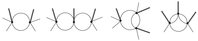
Figure 1: Diagrams at finite $\tau$: every vertex (denoted by a dot) has a source $K$ attached to it (denoted by a double line), besides internal and possibly external legs (denoted by single lines)

What we have done so far in quantum mechanics extends straightforwardly to quantum field theory (at finite $\tau$, on $\Omega=\mathbb{R}^{3}$). The formulas written for a specific frequency $\omega$ can be generalized by assuming that each field depends on the position $\mathbf{x}$ ($z(t)\rightarrow z(t,\mathbf{x})$, $w(t)\rightarrow w(t,\mathbf{x})$, etc.), and that every interaction term is a product among fields, sources $K$ and their derivatives, located at the same point $\mathbf{x}$, integrated in $\mathrm{d}^{3}\mathbf{x}$ on $\mathbb{R}^{3}$.

As far as the quadratic Lagrangian (4.4) is concerned, we must interpret it as

$$\mathcal{L}_{0}(w,\bar{w})\rightarrow\int\mathrm{d}^{3}\mathbf{x}\left[i\bar{w}\sqrt{-\triangle+m^{2}}\dot{w}-i\dot{\bar{w}}\sqrt{-\triangle+m^{2}}w-2\bar{w}(-\triangle+m^{2})w\right],$$ (4.24)

where $\triangle$ denotes the Laplacian. The first two terms in the square brackets are nonlocal, and so may be the interaction terms $\mathcal{L}_{IK}^{w}$, due to $p$ dependence in (4.7). However, these nonlocalities are spurious, because they disappear if we switch to the variables

$$Q\equiv w+\bar{w}=q-z_{0}-\bar{z}_{0},\qquad P\equiv-i\omega(w-\bar{w})=p+i\omega(z_{0}-\bar{z}_{0}),$$ (4.25)

and view the dependencies on $z_{0}$ and $\bar{z}_{0}$ as external sources.

It may be convenient to switch back and forth between the variables $Q$, $P$ and $w$, $\bar{w}$. The former are more convenient for renormalization, because they have a standard power counting. The latter are more clearly related to the initial and final conditions.

Ultimately, the difference between the diagrammatics of quantum field theory at $\tau=\infty$ and the one at $\tau<\infty$ is limited to the external sources $K$. The result is that the diagrams are the same as usual, internally, and obey all the known theorems. They even allow us to generalize the prescription/projection to purely virtual particles, which we discuss in section 9. In the next section we show that the key properties also survive the restriction to a compact space manifold $\Omega$.

5 Compact space manifold

Now we study quantum field theory in a finite interval of time, and on a compact, smooth space manifold $\Omega$. We can study manifolds with a nontrivial boundary $\partial\Omega$, or closed manifolds $\Omega$, such as the sphere or the torus (equivalent to the box with periodic boundary conditions). When $\partial\Omega$ is nontrivial, we assume that the fields $\phi$ satisfy Dirichlet boundary conditions

$$\phi(t,\mathbf{x}_{\partial\Omega})=f(t,\mathbf{x}_{\partial\Omega})$$ (5.1)

on $\partial\Omega$, where $f$ are regular functions and $\mathbf{x}_{\partial\Omega}$ are the space variables restricted to $\partial\Omega$. Problems may appear when $\Omega$ is not smooth (as in the case $\Omega$ = cone), or the boundary conditions (5.1) are singular. These situations must be treated case by case.

We assume that the Lagrangian density depends only on the field $\phi$ and its first derivatives $\partial_{\mu}\phi$, and that each Lagrangian term contains at most two derivatives. Although we write formulas for scalar fields, our formulation is general, and applies to bosons as well as fermions, with obvious modifications. In the case of bosons of higher spins, it is sufficient to view $\phi$ as a multiplet. In the case of gravity, where the curvature tensors $R_{\mu\nu\rho\sigma}$, $R_{\mu\nu}$ and $R$ involve two derivatives $\partial_{\rho}\partial_{\sigma}\phi_{\mu\nu}$ of the fluctuation $\phi_{\mu\nu}$ of the metric tensor $g_{\mu\nu}$ around flat space, we must eliminate them by adding total derivatives to the Lagrangian. This is always possible, since we are assuming that the latter does not depend on higher derivatives of $\phi_{\mu\nu}$, and does not contain terms with more than two derivatives. Later we show how to obtain the correct classical variational problem, once the Lagrangian is rearranged as explained.

For example, in quantum gravity with purely virtual particles, we should not use the higher-derivative formulation “$R+R^{2}+C^{2}$” of [8] (where $C_{\mu\nu\rho\sigma}$ is the Weyl tensor, and $C^{2}$ stands for $C_{\mu\nu\rho\sigma}C^{\mu\nu\rho\sigma}$), which contains Lagrangian terms with four derivatives or less, but the two-derivative formulation of [22], obtained through the introduction of extra fields. Moreover, we should include the total derivatives mentioned above, to make sure that terms like $\phi_{1}\cdots\phi_{n-1}\partial\partial\phi_{n}$ are eliminated in favor of terms like $\phi_{1}\cdots\phi_{n-2}\partial\phi_{n-1}\partial\phi_{n}$. The two-derivative formulation of quantum gravity with purely virtual particles is still renormalizable (at $\tau=\infty$, $\Omega=\mathbb{R}^{3}$; for its renormalizability at $\tau<\infty$, $\Omega$ = compact manifold, see section 6), although not manifestly.

The boundary conditions (5.1) are not straightforward to deal with, since we do not know how to Fourier expand the field. It is better to first shift $\phi$ by any background field $\phi_{0}$ that satisfies the same conditions:

$$\phi(t,\mathbf{x})=\phi_{0}(t,\mathbf{x})+\varphi(t,\mathbf{x}),\qquad\phi_{0}(t,\mathbf{x}_{\partial\Omega})=f(t,\mathbf{x}_{\partial\Omega}),$$ (5.2)

so that the difference $\varphi(t,\mathbf{x})$ satisfies the simplified Dirichlet boundary conditions $\varphi(t,\mathbf{x}_{\partial\Omega})=0$. Note that we are not requiring $\phi_{0}$ to be the solution of a particular differential equation.

Denote the Lagrangian density by

$$L_{\lambda}(\phi,\dot{\phi},\nabla\phi)=L_{0}(\phi,\dot{\phi},\nabla\phi)+L_{I}(\phi,\dot{\phi},\nabla\phi),\qquad L_{0}(\phi,\dot{\phi},\nabla\phi)=\frac{1}{2}\dot{\phi}^{2}-\frac{1}{2}(\nabla\phi)^{2}-\frac{m^{2}}{2}\phi^{2},$$ (5.3)

where the interaction term $L_{I}$ is proportional to a coupling $\lambda$, which is treated perturbatively. After the shift (5.2), we write $L_{\lambda}(\phi,\dot{\phi},\nabla\phi)$ as $\tilde{L}_{\lambda}(\varphi,\dot{\varphi},\nabla\varphi,\phi_{0})$ and obtain

$$\tilde{L}_{\lambda}(\varphi,\dot{\varphi},\nabla\varphi,\phi_{0})=L_{\lambda}(\phi_{0},\dot{\phi}_{0},\nabla\phi_{0})+\varphi A(\phi_{0})+\dot{\varphi}B(\phi_{0})+\nabla(\varphi C(\phi_{0}))+\hat{L}_{\lambda}(\varphi,\dot{\varphi},\nabla\varphi,\phi_{0}),$$ (5.4)

for some functions $A(\phi_{0})$, $B(\phi_{0})$ and $C(\phi_{0})$ of the background field $\phi_{0}$, where the last term $\hat{L}_{\lambda}(\varphi,\dot{\varphi},\nabla\varphi,\phi_{0})=L_{0}(\varphi,\dot{\varphi},\nabla\varphi)+\mathcal{O}(\lambda)$ is at least quadratic in $\varphi$. The first three terms on the right-hand side go unmodified to the generating functional $\Gamma$, while the fourth one disappears when it is integrated on $\Omega$.

5.1 Fourier expansion

Now we expand the shifted field $\varphi(t,\mathbf{x})$ in a basis of eigenfunctions of the Laplacian on $\Omega$.

Let $e_{\mathbf{n}}(\mathbf{x})$, where $\mathbf{n}$ is some label ranging in some set $\mathcal{U}$, denote a complete set of orthonormal eigenstates of the operator $-\triangle+m^{2}$ on $\Omega$, defined by the Dirichlet boundary conditions $e_{\mathbf{n}}(\mathbf{x}_{\partial\Omega})=0$ on $\partial\Omega$ (if $\partial\Omega\neq\oslash$). Let $\omega_{\mathbf{n}}^{2}$ denote their eigenvalues, which are real and positive. The $\varphi$ expansion and the orthonormality relations read

$$\varphi(t,\mathbf{x})=\sum_{\mathbf{n}\in\mathcal{U}}\varphi_{\mathbf{n}}(t)e_{\mathbf{n}}(\mathbf{x})\text{,\qquad}\int_{\Omega}\mathrm{d}^{3}\mathbf{x\hskip 0.72229pt}e_{\mathbf{n}^{\prime}}^{\ast}(\mathbf{x})e_{\mathbf{n}}(\mathbf{x})=\delta_{\mathbf{nn}^{\prime}}.$$ (5.5)

Since we are working with real fields $\varphi$, we can choose a basis of real eigenfunctions. However, in various cases, complex eigenfunctions may be more convenient, because they can highlight the momentum conservation at the vertices. In that case, the complex conjugate $e_{\mathbf{n}}^{\ast}(\mathbf{x})$ of $e_{\mathbf{n}}(\mathbf{x})$ is an eigenfunction with the same eigenvalue $\omega_{\mathbf{n}}^{2}$. Thus, there exists an $\mathbf{n}^{\ast}\in\mathcal{U}$ such that $e_{\mathbf{n}}^{\ast}(\mathbf{x})=$ $e_{\mathbf{n}^{\ast}}(\mathbf{x})$.

In typical cases, $\mathbf{n}^{\ast}=-\mathbf{n}$, but here we want to stay as general as possible. Note that a real $\varphi$ has $\varphi_{\mathbf{n}}^{\ast}(t)=\varphi_{\mathbf{n}^{\ast}}(t)$. The formulas we write look the same with real or complex eigenfunctions: we just have to interpret the range of $\mathbf{n}$ appropriately.

For example, if $\Omega$ is a three torus $T^{3}$, that is to say, a box with periodic boundary conditions, we have

$$e_{\mathbf{n}}(\mathbf{x})=\frac{\mathrm{e}^{i\mathbf{\bar{n}\cdot x}}}{\sqrt{|\Omega|}},\qquad\omega_{\mathbf{n}}=\sqrt{\mathbf{\bar{n}}^{2}+m^{2}},$$ (5.6)

where $|\Omega|=L_{1}L_{2}L_{3}$ is the volume of $\Omega$, $\mathbf{n}=(n_{1},n_{2},n_{3})\in\mathbb{Z}^{3}$, $\mathbf{\bar{n}}=2\pi(n_{1}/L_{1},n_{2}/L_{2},n_{3}/L_{3}\mathbf{)}$ and $L_{1}$, $L_{2}$ and $L_{3}$ are the lengths of the sides of $T^{3}$.

If $\Omega$ is a generic box (with boundary), let $L_{1}/2$, $L_{2}/2$ and $L_{3}/2$ denote the lengths of its sides. The Dirichlet boundary conditions $e_{\mathbf{n}}(\mathbf{x}_{\partial\Omega})=0$ on $\partial\Omega$ give

$$e_{\mathbf{n}}(\mathbf{x})=\sqrt{\frac{8}{|\Omega|}}\prod_{a=1}^{3}\sin\left(\bar{n}_{a}x_{a}\right),\qquad\omega_{\mathbf{n}}=\sqrt{\mathbf{\bar{n}}^{2}+m^{2}},$$ (5.7)

where $\mathbf{n}\in\mathbb{N}_{+}^{3}$.

If $\Omega$ is the sphere $S^{3}$ of radius $R$, we expand $\varphi$ into spherical harmonics $Y^{klm}$ with frequencies

$$\omega_{klm}=\frac{1}{R}\sqrt{k(k+2)+m^{2}R^{2}},$$

where $(k,l,m)\in\mathbb{Z}^{3}$, $k\geqslant l\geqslant 0$, $-l\leqslant m\leqslant l$ [23].

If $\Omega$ is a ball of radius $R$, $e_{\mathbf{n}}(\mathbf{x})$ are proportional to the usual spherical harmonics $Y^{lm}$, times Bessel functions of the first kind:

$$r^{1/2}J_{(2l+1)/2}(kr)Y^{lm}(\theta,\phi),\qquad l\geqslant 0\text{, }-l\leqslant m\leqslant l,$$

where $k\equiv\sqrt{\omega^{2}-m^{2}}$ is fixed by the boundary conditions at $r=R$.

Let us briefly outline the plan from now, before entering into further details. After the Fourier expansion (5.6), we switch to coherent states, to deal with the restriction to finite $\tau$. We obtain a propagator, for the quantum fluctuations, that is unaffected by the initial and final conditions at $t_{\text{i}}$ and $t_{\text{f}}$, and is affected by $\Omega$ only in a minor way. So doing, we manage to develop a formalism that does not alter the spectral optical identities of [2] in a significant way (this aspect will become clear only in section 9). Specifically, we move all the details about the restriction to finite $\tau$ and compact $\Omega$ to the external sectors of the diagrams (apart from the discretizations of the loop momenta, due to the Fourier expansion). The formulation we obtain allows us to study unitarity via the spectral optical identities, and extend the formulation to purely virtual particles.

Before dealing with the complete theory, we treat the quadratic part, and show that the propagator has the form we want.

5.2 Free field theory

For the moment, we concentrate on the free Lagrangian $L_{0}(\varphi,\dot{\varphi},\nabla\varphi)$ for the fluctuation $\varphi$, which coincides with the Lagrangian $\hat{L}_{\lambda}(\varphi,\dot{\varphi},\nabla\varphi,\phi_{0})$ of (5.4) at $\lambda=0$. The integral of $L_{0}(\varphi,\dot{\varphi},\nabla\varphi)$ must be equipped with “endpoint corrections” $\hat{S}_{\text{e}0}$, so that the total gives the correct classical variational problem.

Expanding $\varphi$ as in (5.5), integrating by parts using the $\varphi$ boundary condition $\varphi(t,\mathbf{x}_{\partial\Omega})=0$, and including unspecified endpoint corrections $\hat{S}_{\text{e}}$, we consider the free action

$$\hat{S}_{\text{free}}(\varphi)=\hat{S}_{\text{e}}+\int_{t_{\text{i}}}^{t_{\text{f}}}\mathrm{d}t\int_{\Omega}\mathrm{d}^{3}\mathbf{x}\hskip 0.72229ptL_{0}(\varphi,\dot{\varphi},\nabla\varphi)=\hat{S}_{\text{e}}+\frac{1}{2}\sum_{\mathbf{n}\in\mathcal{U}}\int_{t_{\text{i}}}^{t_{\text{f}}}\mathrm{d}t\hskip 0.72229pt\left(\dot{\varphi}_{\mathbf{n}^{\ast}}\dot{\varphi}_{\mathbf{n}}-\varphi_{\mathbf{n}^{\ast}}\omega_{\mathbf{n}}^{2}\varphi_{\mathbf{n}}\right).$$ (5.8)

Then, we switch to coherent states

$$z_{\mathbf{n}}=\frac{1}{2}\left(\varphi_{\mathbf{n}}+i\frac{\pi_{\mathbf{n}}}{\omega_{\mathbf{n}}}\right),\qquad\bar{z}_{\mathbf{n}}=\frac{1}{2}\left(\varphi_{\mathbf{n}}-i\frac{\pi_{\mathbf{n}}}{\omega_{\mathbf{n}}}\right),$$ (5.9)

by introducing the momenta $\pi_{\mathbf{n}}(t)=\dot{\varphi}_{\mathbf{n}}(t)$ ($\pi_{\mathbf{n}}^{\ast}(t)=\pi_{\mathbf{n}^{\ast}}(t)$), and applying the procedure described in section 4 to each $\mathbf{n}$. We repeat the derivation in detail in the next subsection, when we include the interactions.

We denote the initial and final conditions by $z_{\mathbf{n}}(t_{\text{i}})=z_{\mathbf{n}\text{i}}$, $\bar{z}_{\mathbf{n}}(t_{\text{f}})=\bar{z}_{\mathbf{n}\text{f}}$, and follow the arguments that lead to (4.10). Putting a prime on $\hat{S}_{\text{free}}$, to emphasize that we are working with new variables, the free action is

$$\hat{S}_{\text{free}}^{\prime}=-i\sum_{\mathbf{n}\in\mathcal{U}}\!\left(\bar{z}_{\mathbf{n}^{\ast}\text{f}}\omega_{\mathbf{n}}z_{\mathbf{n}}(t_{\text{f}})+\bar{z}_{\mathbf{n}^{\ast}}(t_{\text{i}})\omega_{\mathbf{n}}z_{\mathbf{n}\text{i}}\right)+\int_{t_{\text{i}}}^{t_{\text{f}}}\!\!\!\mathrm{d}t\!\sum_{\mathbf{n}\in\mathcal{U}}\!\left[i(\bar{z}_{\mathbf{n}^{\ast}}\omega_{\mathbf{n}}\dot{z}_{\mathbf{n}}-\dot{\bar{z}}_{\mathbf{n}^{\ast}}\omega_{\mathbf{n}}z_{\mathbf{n}})-2\bar{z}_{\mathbf{n}^{\ast}}\omega_{\mathbf{n}}^{2}z_{\mathbf{n}}\right]\!,$$ (5.10)

where the first sum on the right-hand side is $\hat{S}_{\text{e}}$.

At this point, we expand the coherent states

$$\bar{z}_{\mathbf{n}}(t)=\bar{z}_{0\mathbf{n}}(t)+\bar{w}_{\mathbf{n}}(t),\qquad z_{\mathbf{n}}(t)=z_{0\mathbf{n}}(t)+w_{\mathbf{n}}(t),$$ (5.11)

around particular solutions

$$z_{0\mathbf{n}}(t)=z_{\mathbf{n}\text{i}}\mathrm{e}^{-i\omega_{\mathbf{n}}(t-t_{\text{i}})},\qquad\bar{z}_{0\mathbf{n}}(t)=\bar{z}_{\mathbf{n}\text{f}}\mathrm{e}^{-i\omega_{\mathbf{n}}(t_{\text{f}}-t)},$$ (5.12)

of the free equations with the same initial and final conditions,

$$i\dot{z}_{0\mathbf{n}}-\omega_{\mathbf{n}}z_{0\mathbf{n}}=0,\qquad-i\dot{\bar{z}}_{0\mathbf{n}}-\omega_{\mathbf{n}}\bar{z}_{0\mathbf{n}}=0,\qquad z_{0\mathbf{n}}(t_{\text{i}})=z_{\mathbf{n}\text{i}},\qquad\bar{z}_{0\mathbf{n}}(t_{\text{f}})=\bar{z}_{\mathbf{n}\text{f}},$$ (5.13)

so that the quantum fluctuations $\bar{w}_{\mathbf{n}}$, $w_{\mathbf{n}}$ satisfy simpler initial and final conditions:

$$w_{\mathbf{n}}(t_{\text{i}})=\bar{w}_{\mathbf{n}}(t_{\text{f}})=0.$$ (5.14)

The free action is finally

$$S_{\text{free}}(w,\bar{w})=-2i\sum_{\mathbf{n}\in\mathcal{U}}\bar{z}_{\mathbf{n}^{\ast}\text{f}}\omega_{\mathbf{n}}\mathrm{e}^{-i\omega_{\mathbf{n}}\tau}z_{\mathbf{n}\text{i}}+\int_{t_{\text{i}}}^{t_{\text{f}}}\mathrm{d}t\sum_{\mathbf{n}\in\mathcal{U}}\hskip 0.72229pt\left[i(\bar{w}_{\mathbf{n}^{\ast}}\omega_{\mathbf{n}}\dot{w}_{\mathbf{n}}-\dot{\bar{w}}_{\mathbf{n}^{\ast}}\omega_{\mathbf{n}}w_{\mathbf{n}})-2\bar{w}_{\mathbf{n}^{\ast}}\omega_{\mathbf{n}}^{2}w_{\mathbf{n}}\right],$$ (5.15)

and the $w$ propagators read

$$\langle w_{\mathbf{n}}(e)\bar{w}_{\mathbf{n}^{\prime}}(-e)\rangle_{c}^{\text{free}}=\frac{i\delta_{\mathbf{n}^{\ast}\mathbf{n}^{\prime}}}{2\omega(e-\omega_{\mathbf{n}}+i\epsilon)},\qquad\langle w_{\mathbf{n}}(e)w_{\mathbf{n}^{\prime}}(-e)\rangle_{c}^{\text{free}}=\langle\bar{w}_{\mathbf{n}}(e)\bar{w}_{\mathbf{n}^{\prime}}(-e)\rangle_{c}^{\text{free}}=0,$$ (5.16)

after Fourier transform, where the subscript $c$ means “connected”. We have inserted it to use the formulas (5.16) below. Note that, due to finite volume effects (the linear terms of (5.4), which are proportional to $A$ and $B$), the full $w$-$\bar{w}$ free propagator does not coincide with the connected part of the $z$-$\bar{z}$ one.

As expected, the propagators do not know of the initial and final conditions. Moreover, they know of $\Omega$ only through the discretization of the frequencies and the momenta.

5.3 Interacting theory

Starting over from (5.4), the total action can be written as

$$\mathcal{S}_{\lambda}(\varphi,\phi_{0}) = \mathcal{S}_{\text{e}}+\int_{t_{\text{i}}}^{t_{\text{f}}}\!\!\mathrm{d}t\!\int_{\Omega}\!\mathrm{d}^{3}\mathbf{x\hskip 0.72229pt}L_{\lambda}(\phi,\dot{\phi},\nabla\phi)=\int_{t_{\text{i}}}^{t_{\text{f}}}\!\!\mathrm{d}t\!\int_{\Omega}\!\mathrm{d}^{3}\mathbf{x\hskip 0.72229pt}L_{\lambda}(\phi_{0},\dot{\phi}_{0},\nabla\phi_{0})+\mathcal{\hat{S}}_{\lambda}(\varphi,\phi_{0}),$$

$$\mathcal{\hat{S}}_{\lambda}(\varphi,\phi_{0}) = \mathcal{S}_{\text{e}}+\int_{t_{\text{i}}}^{t_{\text{f}}}\!\!\mathrm{d}t\!\int_{\Omega}\!\mathrm{d}^{3}\mathbf{x\hskip 0.72229pt}\left[\hat{L}_{\lambda}(\varphi,\dot{\varphi},\nabla\varphi,\phi_{0})+\varphi A(\phi_{0})+\dot{\varphi}B(\phi_{0})\right],$$ (5.17)

where $\mathcal{S}_{\text{e}}$ collects the endpoint and boundary corrections that must be included to have the correct classical variational problem.

After the Fourier expansion (5.5), we have

$$\mathcal{\hat{S}}_{\lambda}(\varphi,\phi_{0}) = \mathcal{S}_{\text{e}}+\int_{t_{\text{i}}}^{t_{\text{f}}}\!\mathrm{d}t\!\hskip 1.4457pt\check{L}_{\lambda}(\varphi_{\mathbf{n}},\dot{\varphi}_{\mathbf{n}},\phi_{0}),$$

$$\check{L}_{\lambda}(\varphi_{\mathbf{n}},\dot{\varphi}_{\mathbf{n}},\phi_{0}) \equiv \int_{\Omega}\!\mathrm{d}^{3}\mathbf{x\hskip 0.72229pt}\left[\hat{L}_{\lambda}(\varphi,\dot{\varphi},\nabla\varphi,\phi_{0})+\varphi A(\phi_{0})+\dot{\varphi}B(\phi_{0})\right].$$

Defining

$$A_{\mathbf{n}^{\ast}}\equiv\int_{\Omega}\!\mathrm{d}^{3}\mathbf{x}\hskip 0.72229ptA(\phi_{0})e_{\mathbf{n}}(\mathbf{x}),\qquad B_{\mathbf{n}^{\ast}}\equiv\int_{\Omega}\!\mathrm{d}^{3}\mathbf{x}\hskip 0.72229ptB(\phi_{0})e_{\mathbf{n}}(\mathbf{x}),$$

and separating the interactions $\check{L}_{I}(\varphi_{\mathbf{n}},\dot{\varphi}_{\mathbf{n}},\phi_{0})$ from the rest, we write

$$\check{L}_{\lambda}(\varphi_{\mathbf{n}},\dot{\varphi}_{\mathbf{n}},\phi_{0})\equiv\frac{1}{2}\sum_{\mathbf{n}\in\mathcal{U}}\left(\dot{\varphi}_{\mathbf{n}^{\ast}}\dot{\varphi}_{\mathbf{n}}-\varphi_{\mathbf{n}^{\ast}}\omega_{\mathbf{n}}^{2}\varphi_{\mathbf{n}}+2A_{\mathbf{n}^{\ast}}\varphi_{\mathbf{n}}+2B_{\mathbf{n}^{\ast}}\dot{\varphi}_{\mathbf{n}}\right)+\check{L}_{I}(\varphi_{\mathbf{n}},\dot{\varphi}_{\mathbf{n}},\phi_{0}).$$

Note that $\phi_{0}$, $A(\phi_{0})$ and $B(\phi_{0})$ may not admit an acceptable expansion in the basis $e_{\mathbf{n}}(\mathbf{x})$, within the same space of functions as $\varphi$ does. Nevertheless, we do not need to interpret $A_{\mathbf{n}^{\ast}}$ and $B_{\mathbf{n}^{\ast}}$ as coefficients of a Fourier expansion. It is enough to view them as the integrals shown. So doing, we can include the effects of $\phi_{0}$ into the external sources $K_{0}$ (see below).

Then, we introduce the Hamiltonian

$$H_{\lambda}(\pi_{\mathbf{n}},\varphi_{\mathbf{n}},\phi_{0})=\sum_{\mathbf{n}\in\mathcal{U}}\pi_{\mathbf{n}^{\ast}}\dot{\varphi}_{\mathbf{n}}-\check{L}_{\lambda}(\varphi_{\mathbf{n}},\dot{\varphi}_{\mathbf{n}},\phi_{0}),$$

where the momenta are

$$\pi_{\mathbf{n}}=\dot{\varphi}_{\mathbf{n}}+B_{\mathbf{n}}+\Delta_{\mathbf{n}},\qquad\Delta_{\mathbf{n}}\equiv\frac{\partial\check{L}_{I}(\varphi_{\mathbf{n}},\dot{\varphi}_{\mathbf{n}},\phi_{0})}{\partial\dot{\varphi}_{\mathbf{n}^{\ast}}},$$

and switch to the action

$$\mathcal{\hat{S}}_{\lambda}(\varphi,\phi_{0})=\mathcal{S}_{\text{e}}^{\prime}+\int_{t_{\text{i}}}^{t_{\text{f}}}\!\mathrm{d}t\!\hskip 1.4457ptL_{\lambda}^{\prime}(\varphi_{\mathbf{n}},\dot{\varphi}_{\mathbf{n}},\pi_{\mathbf{n}},\dot{\pi}_{\mathbf{n}},\phi_{0}),$$ (5.18)

by means of the equivalent Lagrangian

$$L_{\lambda}^{\prime}(\varphi_{\mathbf{n}},\dot{\varphi}_{\mathbf{n}},\pi_{\mathbf{n}},\dot{\pi}_{\mathbf{n}},\phi_{0}) = \frac{1}{2}\sum_{\mathbf{n}\in\mathcal{U}}(\pi_{\mathbf{n}^{\ast}}\dot{\varphi}_{\mathbf{n}}-\dot{\pi}_{\mathbf{n}^{\ast}}\varphi_{\mathbf{n}})-H_{\lambda}(\pi_{\mathbf{n}},\varphi_{\mathbf{n}},\phi_{0}),$$

$$= \frac{1}{2}\sum_{\mathbf{n}\in\mathcal{U}}(\pi_{\mathbf{n}^{\ast}}\dot{\varphi}_{\mathbf{n}}-\dot{\pi}_{\mathbf{n}^{\ast}}\varphi_{\mathbf{n}}-\pi_{\mathbf{n}^{\ast}}\pi_{\mathbf{n}}-\varphi_{\mathbf{n}^{\ast}}\omega_{\mathbf{n}}^{2}\varphi_{\mathbf{n}})$$

$$+\frac{1}{2}\sum_{\mathbf{n}\in\mathcal{U}}(2B_{\mathbf{n}^{\ast}}\pi_{\mathbf{n}}+2A_{\mathbf{n}^{\ast}}\varphi_{\mathbf{n}}-B_{\mathbf{n}^{\ast}}B_{\mathbf{n}})+L_{I}(\pi_{\mathbf{n}},\varphi_{\mathbf{n}},\phi_{0}),$$

and possibly different endpoint corrections $\mathcal{S}_{\text{e}}^{\prime}$. The interaction part reads

$$L_{I}(\pi_{\mathbf{n}},\varphi_{\mathbf{n}},\phi_{0})=\check{L}_{I}(\varphi_{\mathbf{n}},\dot{\varphi}_{\mathbf{n}},\phi_{0})+\frac{1}{2}\sum_{\mathbf{n}\in\mathcal{U}}\Delta_{\mathbf{n}^{\ast}}\Delta_{\mathbf{n}}.$$

Finally, we switch to coherent states $z_{\mathbf{n}}$, $\bar{z}_{\mathbf{n}}$ by means of (5.9), and to the quantum fluctuations $w_{\mathbf{n}}$ and $\bar{w}_{\mathbf{n}}$ by means of the shift (5.11).

Now we are ready to determine the corrections $\mathcal{S}_{\text{e}}^{\prime}$, so as to have the correct classical variational problem. They may depend on the initial, final and possibly boundary conditions (5.1). Defining

$$z(t,\mathbf{x})=\sum_{\mathbf{n}\in\mathcal{U}}z_{\mathbf{n}}(t)e_{\mathbf{n}}(\mathbf{x}),\qquad\bar{z}(t,\mathbf{x})=\sum_{\mathbf{n}\in\mathcal{U}}\bar{z}_{\mathbf{n}}(t)e_{\mathbf{n}}(\mathbf{x}),$$ (5.20)

the initial and final conditions are

$$z(t_{\text{i}},\mathbf{x})=z_{\text{i}}(\mathbf{x})\equiv\sum_{\mathbf{n}\in\mathcal{U}}z_{\mathbf{n}\text{i}}e_{\mathbf{n}}(\mathbf{x}),\qquad\bar{z}(t_{\text{f}},\mathbf{x})=\bar{z}_{\text{f}}(\mathbf{x})\equiv\sum_{\mathbf{n}\in\mathcal{U}}\bar{z}_{\mathbf{n}\text{f}}e_{\mathbf{n}}(\mathbf{x}),$$ (5.21)

where $z_{\text{i}}(\mathbf{x})$ and $\bar{z}_{\text{f}}(\mathbf{x})$ are given functions on $\Omega$. Note that they vanish on $\partial\Omega$, which makes them compatible with the boundary conditions (5.1).

It is easy to check that the correct endpoint action is

$$\mathcal{S}_{\text{e}}^{\prime}=\hat{S}_{\text{e}}=-i\sum_{\mathbf{n}\in\mathcal{U}}\!\left(\bar{z}_{\mathbf{n}^{\ast}\text{f}}\omega_{\mathbf{n}}z_{\mathbf{n}}(t_{\text{f}})+\bar{z}_{\mathbf{n}^{\ast}}(t_{\text{i}})\omega_{\mathbf{n}}z_{\mathbf{n}\text{i}}\right).$$ (5.22)

The first thing to notice is that the Lagrangian $L_{\lambda}^{\prime}$ of (5.3) depends on the time derivatives $\dot{\varphi}_{\mathbf{n}}$ in a very simple way. At the same time, the gradients of the fields have disappeared after the Fourier expansion ($\pi_{\mathbf{n}}$, $\varphi_{\mathbf{n}}$, $z_{\mathbf{n}}$ and $\bar{z}_{\mathbf{n}}$ depend only on time). In particular, the interaction Lagrangian $L_{I}(\pi_{\mathbf{n}},\varphi_{\mathbf{n}},\phi_{0})$ does not contain time derivatives $\dot{z}_{\mathbf{n}}$ and $\dot{\bar{z}}_{\mathbf{n}}$, after the switch to coherent states. Thus, when we study the variations $\delta z_{\mathbf{n}}$, $\delta\bar{z}_{\mathbf{n}}$ of $z_{\mathbf{n}}$ and $\bar{z}_{\mathbf{n}}$, the endpoint contributions are compensated by the same endpoint corrections we had in the free-field limit, as in (5.10).

5.4 Complete action

The final action (5.17) is, from (5.18), (5.3) and (5.22)

$$S_{\lambda}(w,\bar{w})\equiv\mathcal{S}_{\lambda}(\varphi,\phi_{0})=\int_{t_{\text{i}}}^{t_{\text{f}}}\mathrm{d}t\int_{\Omega}\mathrm{d}^{3}\mathbf{x\hskip 0.72229pt}L_{\lambda}(\phi_{0},\dot{\phi}_{0},\nabla\phi_{0})+\hat{S}_{\text{free}}^{\prime}$$

$$\qquad+\frac{1}{2}\int_{t_{\text{i}}}^{t_{\text{f}}}\mathrm{d}t\mathbf{\hskip 0.72229pt}\sum_{\mathbf{n}\in\mathcal{U}}(2B_{\mathbf{n}^{\ast}}\pi_{\mathbf{n}}+2A_{\mathbf{n}^{\ast}}\varphi_{\mathbf{n}}-B_{\mathbf{n}^{\ast}}B_{\mathbf{n}})+\int_{t_{\text{i}}}^{t_{\text{f}}}\mathrm{d}t\mathbf{\hskip 0.72229pt}\mathcal{L}_{I}(z_{\mathbf{n}},\bar{z}_{\mathbf{n}}),\,\qquad$$ (5.23)

where $\mathcal{L}_{I}(z_{\mathbf{n}},\bar{z}_{\mathbf{n}})=L_{I}(\pi_{\mathbf{n}},\varphi_{\mathbf{n}},\phi_{0})$, with the substitutions $\pi_{\mathbf{n}}=-i\omega_{\mathbf{n}}(z_{\mathbf{n}}-\bar{z}_{\mathbf{n}})$, $\varphi_{\mathbf{n}}=z_{\mathbf{n}}+\bar{z}_{\mathbf{n}}$, and $\hat{S}_{\text{free}}^{\prime}$ is the expression of formula (5.10). It is understood that the relations between $z_{\mathbf{n}}$, $\bar{z}_{\mathbf{n}}$ and $w_{\mathbf{n}}$, $\bar{w}_{\mathbf{n}}$ are still given by the shift (5.11), defined by the free-field solution (5.12) with initial/final conditions (5.13). This way, $\hat{S}_{\text{free}}^{\prime}$ coincides with the free $w$, $\bar{w}$ action $S_{\text{free}}(w,\bar{w})$ of formula (5.15).

We see that $S_{\lambda}(w,\bar{w})$ is made of three types of contributions: $i$) those that go unmodified into the generating functional $\Gamma$, which are the first term after the equal sign in the first line, and the sum in the second line; $ii$) the free part, which is (5.15) and gives the propagators (5.16); $iii$) the interaction part, encoded in $\mathcal{L}_{I}(z_{\mathbf{n}},\bar{z}_{\mathbf{n}})$. For the calculations, we can concentrate on the last two terms.

5.5 Amplitudes, correlation functions, and diagrams

The amplitudes we want to calculate are

$$\langle\bar{z}_{\text{f}},t_{\text{f}};z_{\text{i}},t_{\text{i}}\rangle_{\zeta,\bar{\zeta}} = \!\!\!\!\!\!\!\!\underset{z(t_{\text{i}})=z_{\text{i}},\hskip 0.72229pt\bar{z}(t_{\text{f}})=\bar{z}_{\text{f}}}{\int}\!\!\!\!\!\!\!\![\mathrm{d}z\mathrm{d}\bar{z}]\,\mathrm{\exp}\left(iS_{\lambda}(w,\bar{w})+i\int_{t_{\text{i}}}^{t_{\text{f}}}\mathrm{d}t\hskip 0.72229pt\int_{\Omega}\!\mathrm{d}^{3}\mathbf{x}(\bar{\zeta}z+\bar{z}\zeta)\right)$$ (5.24)

$$= \!\!\!\!\!\!\!\!\underset{w(t_{\text{i}})=\bar{w}(t_{\text{f}})=0}{\int}\!\!\!\!\!\!\!\![\mathrm{d}w\mathrm{d}\bar{w}]\,\mathrm{\exp}\left(iS_{\lambda}(w,\bar{w})+i\int_{t_{\text{i}}}^{t_{\text{f}}}\mathrm{d}t\hskip 0.72229pt\int_{\Omega}\!\mathrm{d}^{3}\mathbf{x}(\bar{\zeta}z_{0}+\bar{z}_{0}\zeta+\bar{\zeta}w+\bar{w}\zeta)\right)\!\!,\qquad\quad$$

where $w(t,\mathbf{x})$, $\bar{w}(t,\mathbf{x})$, $z_{0}(t,\mathbf{x})$ and $\bar{z}_{0}(t,\mathbf{x})$ are defined from their Fourier coefficients in analogy with (5.20). As usual, we have introduced sources $\zeta$, $\bar{\zeta}$, to prepare for the diagrammatic approach. The initial and final “states” are described by the configurations (5.21), which are compatible with the boundary conditions (5.1).

At $\mathcal{L}_{I}(z_{\mathbf{n}},\bar{z}_{\mathbf{n}})=0$ (which we call “free limit”, although some $\lambda$ dependence remains in $A$, $B$ and $L_{\lambda}(\phi_{0},\dot{\phi}_{0},\nabla\phi_{0})$), we find, using (5.23),

$$\langle\bar{z}_{\text{f}},t_{\text{f}};z_{\text{i}},t_{\text{i}}\rangle_{\zeta,\bar{\zeta}}^{\text{free}}=\exp\left(i\tilde{W}_{0}+i\hat{W}_{0}(\zeta^{\prime},\bar{\zeta}^{\prime})+i\int_{t_{\text{i}}}^{t_{\text{f}}}\!\!\mathrm{d}t\!\int_{\Omega}\!\mathrm{d}^{3}\mathbf{x\hskip 0.72229pt(}\bar{\zeta}^{\prime}z_{0}+\bar{z}_{0}\zeta^{\prime})\right)\equiv\mathrm{e}^{iW^{\text{free}}},$$ (5.25)

where

$$\zeta^{\prime}=\zeta+A+i\omega B,\qquad\bar{\zeta}^{\prime}=\bar{\zeta}+A-iB\omega,$$ (5.26)

and, from (4.14) and (4.19),

$$\tilde{W}_{0} = \int_{t_{\text{i}}}^{t_{\text{f}}}\!\!\mathrm{d}t\!\int_{\Omega}\!\mathrm{d}^{3}\mathbf{x}\left[\mathbf{\hskip 0.72229pt}L_{\lambda}(\phi_{0},\dot{\phi}_{0},\nabla\phi_{0})-\frac{1}{2}B^{2}(\phi_{0})\right],$$

$$\hat{W}_{0}(\zeta,\bar{\zeta}) = -2i\sum_{\mathbf{n}\in\mathcal{U}}\bar{z}_{\mathbf{n}^{\ast}\text{f}}\omega_{\mathbf{n}}\mathrm{e}^{-i\omega_{\mathbf{n}}\tau}z_{\mathbf{n}\text{i}}+i\int_{t_{\text{i}}}^{t_{\text{f}}}\!\!\mathrm{d}t\!\!\int_{t_{\text{i}}}^{t_{\text{f}}}\!\!\mathrm{d}t^{\prime}\!\sum_{\mathbf{n}\in\mathcal{U}}\bar{\zeta}_{\mathbf{n}^{\ast}}(t)\theta(t-t^{\prime})\frac{\mathrm{e}^{-i\omega_{\mathbf{n}}(t-t^{\prime})}}{2\omega_{\mathbf{n}}}\zeta_{\mathbf{n}}(t^{\prime}).\qquad$$ (5.27)

In (5.26) $\omega$ stands for the operator $\sqrt{-\triangle+m^{2}}$, where the derivatives act away from $B$. In (5.27) $\zeta_{\mathbf{n}}$ and $\bar{\zeta}_{\mathbf{n}}$ are the coefficients of the Fourier expansion of $\zeta$ and $\bar{\zeta}$ (which we can assume to make sense, since the sources couple to $\bar{z}$ and $z$). We have moved the infinite contribution $-(\tau/2)\sum_{\mathbf{n}\in\mathcal{U}}\omega_{\mathbf{n}}$ into the normalization of the functional integral.

Switching $\mathcal{L}_{I}(z_{\mathbf{n}},\bar{z}_{\mathbf{n}})$ back on, the amplitudes of the interacting theory are

$$\langle\bar{z}_{\text{f}},t_{\text{f}};z_{\text{i}},t_{\text{i}}\rangle_{\zeta,\bar{\zeta}}=\exp\left(i\int_{t_{\text{i}}}^{t_{\text{f}}}\!\!\mathrm{d}t\mathbf{\hskip 1.4457pt}\mathcal{L}_{I}\left(\frac{\delta}{i\delta\bar{\zeta}_{\mathbf{n}^{\ast}}},\frac{\delta}{i\delta\zeta_{\mathbf{n}^{\ast}}}\right)\right)\mathrm{e}^{iW^{\text{free}}}.$$ (5.28)

So far, we have tacitly assumed $t_{\text{f}}>t_{\text{i}}$. For $t_{\text{i}}>t_{\text{f}}$, we have

$$\langle\bar{z}_{\text{f}},t_{\text{f}};z_{\text{i}},t_{\text{i}}\rangle_{\zeta,\bar{\zeta}}=\langle\bar{z}_{\text{i}},t_{\text{i}};z_{\text{f}},t_{\text{f}}\rangle_{\zeta,\bar{\zeta}}^{\ast},$$ (5.29)

from (2.6).

The correlation functions are

$$\langle\bar{z}_{\text{f}},t_{\text{f}}|\hskip 0.72229pt\tilde{z}_{\mathbf{n}_{1}}(t_{1})\cdots\tilde{z}_{\mathbf{n}_{k}}(t_{k})|\hskip 0.72229ptz_{\text{i}},t_{\text{i}}\rangle\equiv\left.\frac{\delta^{k}\langle\bar{z}_{\text{f}},t_{\text{f}};z_{\text{i}},t_{\text{i}}\rangle_{\zeta,\bar{\zeta}}}{i\delta\tilde{\zeta}_{\mathbf{n}_{1}^{\ast}}(t_{1})\cdots i\delta\tilde{\zeta}_{\mathbf{n}_{k}^{\ast}}(t_{n})}\right|_{\zeta=\bar{\zeta}=0}\!\!\!\!\!,$$ (5.30)

where $\tilde{z}_{\mathbf{n}_{j}}(t_{j})$ and $\tilde{\zeta}_{\mathbf{n}_{j}^{\ast}}(t_{j})$ may stand for $z_{\mathbf{n}_{j}}(t_{j})$ and $\bar{\zeta}_{\mathbf{n}_{j}^{\ast}}(t_{j})$, or $\bar{z}_{\mathbf{n}_{j}}(t_{j})$ and $\zeta_{\mathbf{n}_{j}^{\ast}}(t_{j})$. Although the amplitudes $\langle\bar{z}_{\text{f}},t_{\text{f}};z_{\text{i}},t_{\text{i}}\rangle$ have no external legs, since they are evaluated at $\zeta=\bar{\zeta}=0$, the correlation functions are useful for the diagrammatic calculations, since propagators and subdiagrams are particular cases of diagrams with external legs. It is understood that the correlation functions (5.30) vanish when an insertion $\tilde{z}_{\mathbf{n}_{j}}(t_{j})$ lies outside the time interval $(t_{\text{i}},t_{\text{f}})$.

Note that the correlation functions (5.30) receive contributions from all the diagrams, including those that factorize subdiagrams with no external legs. By definition, the connected correlation functions do not include those types of diagrams.

We see that, ultimately, the $\tilde{\zeta}$ derivatives of (5.30) and (5.28) act on the free amplitude $\mathrm{e}^{iW^{\text{free}}}$, where $W^{\text{free}}$ is encoded in formulas (5.25) and (5.27). Since $W^{\text{free}}$ is the exponential of a quadratic form in the sources $\tilde{\zeta}$, the derivatives bring down propagators or endpoints. The endpoints are the normalized one-point function

$$\left.\mathrm{e}^{-iW^{\text{free}}}\frac{\delta\mathrm{e}^{iW^{\text{free}}}}{i\delta\bar{\zeta}_{\mathbf{n}^{\ast}}(t)}\right|_{\zeta=\bar{\zeta}=0}=z_{0\mathbf{n}}(t)+i\int_{t_{\text{i}}}^{t_{\text{f}}}\!\!\mathrm{d}t^{\prime}\hskip 1.4457pt\theta(t-t^{\prime})\frac{\mathrm{e}^{-i\omega_{\mathbf{n}}(t-t^{\prime})}}{2\omega_{\mathbf{n}}}(A_{\mathbf{n}}(t^{\prime})+i\omega_{\mathbf{n}}B_{\mathbf{n}}(t^{\prime})),$$ (5.31)

and a similar expression for $-i\left.\mathrm{e}^{-iW^{\text{free}}}\delta\mathrm{e}^{iW^{\text{free}}}/\delta\zeta_{\mathbf{n}}(t)\right|_{\zeta=\bar{\zeta}=0}$. We see that both the restriction to finite $\tau$ and the one to compact $\Omega$ contribute to the endpoints.

By repeatedly differentiating $\mathrm{e}^{iW^{\text{free}}}$, we can build the diagrams, and, ultimately, calculate any amplitude $\langle\bar{z}_{\text{f}},t_{\text{f}};z_{\text{i}},t_{\text{i}}\rangle$ we want, perturbatively and diagrammatically. In fig. 2 we illustrate the diagrams with two and three cubic vertices, and no external legs. The double lines stand for the sources $K$, while the little circles stand for the endpoints (8.11). The internal lines are the propagators (5.16), while the vertices are studied below.

From what we have said, it follows that, in the end, the diagrams look like the ones we are accustomed to at $\tau=\infty$, $\Omega=\mathbb{R}^{3}$, at least internally, apart from the discretization of the loop momenta. Externally, the sources $K$ attached to the vertices take care of the restrictions to finite $\tau$ and compact $\Omega$. These properties are going to be extremely useful to study unitarity and extend the formulation to purely virtual particles.

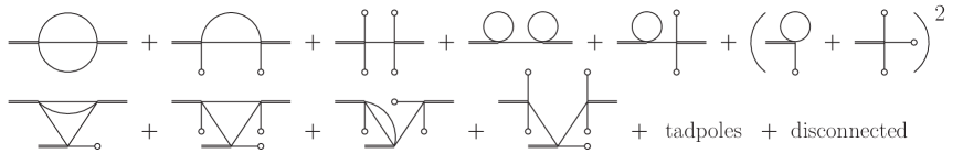
Figure 2: Diagrams with two and three cubic vertices

5.6 Vertices

Going through the derivation just outlined, we see that the vertices have the form

$$\int_{t_{\text{i}}}^{t_{\text{f}}}\mathrm{d}t\int_{\Omega}\mathrm{d}^{3}\mathbf{x\hskip 0.72229pt}K(t,\mathbf{x})Q^{i}P^{j}\overset{k}{\overbrace{\nabla Q\cdots\nabla Q}}\mathbf{\hskip 2.8903pt}\overset{l}{\overbrace{\nabla P\cdots\nabla P}},$$ (5.32)

where, as in (4.25),

$$Q(t,\mathbf{x})=\sum_{\mathbf{n}\in\mathcal{U}}\left(w_{\mathbf{n}}(t)+\bar{w}_{\mathbf{n}}(t)\right)e_{\mathbf{n}}(\mathbf{x}),\qquad P(t,\mathbf{x})=-i\sum_{\mathbf{n}\in\mathcal{U}}\omega_{\mathbf{n}}\left(w_{\mathbf{n}}(t)-\bar{w}_{\mathbf{n}}(t)\right)e_{\mathbf{n}}(\mathbf{x}),$$ (5.33)

while the source $K(t,\mathbf{x})$ is built with $z_{0}$, $\bar{z}_{0}$ and $\phi_{0}$. Defining the constants

$$C_{\mathbf{n}_{1}\cdots\mathbf{n}_{k}}^{K\mathbf{m}_{1}\cdots\mathbf{m}_{l}}(t)=i^{-l}|\Omega|^{(k+l-2)/2}\int_{\Omega}\mathrm{d}^{3}\mathbf{x\hskip 0.72229pt}K(t,\mathbf{x})e_{\mathbf{n}_{1}}(\mathbf{x})\cdots e_{\mathbf{n}_{k}}(\mathbf{x})\nabla e_{\mathbf{m}_{1}}(\mathbf{x})\cdots\nabla e_{\mathbf{m}_{l}}(\mathbf{x}),$$ (5.34)

the vertices can be arranged as

$$i^{k+l}|\Omega|^{v}\sum_{\mathbf{n},\mathbf{m}}\Pi\omega\int_{t_{\text{i}}}^{t_{\text{f}}}\!\!\mathrm{d}t\hskip 0.72229ptC_{\mathbf{n}_{1}\cdots\mathbf{n}_{i+j}}^{K\mathbf{m}_{1}\cdots\mathbf{m}_{k+l}}w_{\mathbf{n}_{1}}\cdots w_{\mathbf{n}_{i}}\bar{w}_{\mathbf{m}_{1}}\cdots\bar{w}_{\mathbf{m}_{k}}w_{\mathbf{n}_{i+1}}\cdots w_{\mathbf{n}_{i+j}}\bar{w}_{\mathbf{m}_{k+1}}\cdots\bar{w}_{\mathbf{m}_{k+l}},\quad$$ (5.35)

where $v=(2-i-j-k-l)/2$ and $\Pi\omega$ stands for a product of frequencies $\omega_{\mathbf{n}}$, $\omega_{\mathbf{m}}$.

Let us examine some typical situations, focusing on $\Pi\omega=1$ and $K\equiv 1$, and dropping the superscript $K$ in $C$.

If $\Omega$ is a three torus $T^{3}$, we find

$$C_{\mathbf{n}_{1}\cdots\mathbf{n}_{i}}^{\mathbf{n}_{i+1}\cdots\mathbf{n}_{i+j}}=\mathbf{\bar{n}}_{i+1}\cdots\mathbf{\bar{n}}_{i+j}\mathbf{\delta}(\mathbf{n}_{1}+\cdots+\mathbf{n}_{i+j}),\qquad\mathbf{\delta}(\mathbf{n})=\left\{\begin{tabular}[]{l}$1$ if $\mathbf{n}=\mathbf{0},$\\ $0$ otherwise,\end{tabular}\right.$$ (5.36)

so the discretized momentum is conserved at the vertices.

If $\Omega$ is a bounded box, the discretized momentum is not conserved at the vertices. We can gain a form of momentum conservation by introducing external sources $K$ to take care of the restriction to finite volume, similar to the sources $K_{n\alpha}$ introduced in (2.15) for the restriction to finite $\tau$. For simplicity, we focus on vertices that do not involve gradients, since it is straightforward to generalize the results to include them.

We double the sides of the box by writing a typical vertex as

$$\int_{t_{\text{i}}}^{t_{\text{f}}}\mathrm{d}t\int_{\Omega}\mathrm{d}^{3}\mathbf{x\hskip 0.72229pt}w^{i}\bar{w}^{j}=\int_{t_{\text{i}}}^{t_{\text{f}}}\mathrm{d}t\left(\prod_{a=1}^{3}\int_{0}^{L_{a}}\mathrm{d}x_{a}\right)K(\mathbf{x})w^{i}\bar{w}^{j},$$

where $K(\mathbf{x})=\prod_{a=1}^{3}\theta(L_{a}-2x_{a})$. Moreover, we use

$$e_{\mathbf{n}}(\mathbf{x})=\frac{i}{\sqrt{L_{1}L_{2}L_{3}}}\prod_{a=1}^{3}(\mathrm{e}^{i\bar{n}_{a}x_{a}}-\mathrm{e}^{-i\bar{n}_{a}x_{a}})\equiv\sum_{\pi(\mathbf{n})}c_{\pi(\mathbf{n})}f_{\pi(\mathbf{n})}(\mathbf{x}),\qquad f_{\mathbf{n}}(\mathbf{x})\equiv\frac{\mathrm{e}^{i\mathbf{\bar{n}\cdot x}}}{\sqrt{L_{1}L_{2}L_{3}}},$$

to switch to the basis $f_{\mathbf{n}}(\mathbf{x})$ with periodic boundary conditions, where $c_{\pi(\mathbf{n})}=\pm i$ are certain coefficients, and the label $\pi(\mathbf{n})$ collects all the ways $(\pm n_{1},\pm n_{2},\pm n_{3})$ of flipping the signs in front of the integer numbers. We obtain

$$\int_{\Omega}\mathrm{d}^{3}\mathbf{x\hskip 0.72229pt}w^{i}\bar{w}^{j}\propto\sum_{\mathbf{n}_{0},\mathbf{n}_{1}\cdots\mathbf{n}_{i+j}}\left[\sum_{\pi(\mathbf{n})}\mathbf{\delta}\!\left(\mathbf{n}_{0}+\sum_{k=1}^{i+j}\pi(\mathbf{n}_{k})\right)\prod_{k=1}^{i+j}c_{\pi(\mathbf{n}_{k})}\right]K_{\mathbf{n}_{0}}w_{\mathbf{n}_{1}}\cdots w_{\mathbf{n}_{i}}\bar{w}_{\mathbf{n}_{i+1}}\cdots\bar{w}_{\mathbf{n}_{i+j}},$$

where

$$K_{\mathbf{n}}=\left(\prod_{a=1}^{3}\int_{0}^{L_{a}}\mathrm{d}x_{a}\right)\mathbf{\hskip 0.72229pt}f_{\mathbf{n}}^{\ast}(\mathbf{x})K(\mathbf{x}).$$

We see that now we have momentum conservation at the vertices, provided we take into account the momentum carried by $K_{\mathbf{n}}$.

Each vertex can be imagined as a sum (the one in square brackets) of usual vertices coupled to external sources. A diagram with $I$ internal legs splits into a sum of copies that have identical propagators, but different vertices, which correspond to the choices of signs in front of the components of the internal momenta.

If $\Omega$ is the sphere $S^{3}$, the boundary is absent. Invariance under translations on the sphere means that there is no reflection, and the (angular) momentum is conserved. The coefficients $C_{\mathbf{n}_{1}\cdots\mathbf{n}_{i}}^{K\mathbf{m}_{1}\cdots\mathbf{m}_{j}}$ can be worked out from the decomposition of the product of two (or more) spherical harmonics in the same basis of spherical harmonics.

If $\Omega$ is a ball $B$, the angular momentum is conserved, but the boundary originates a reflection. It is easier to first consider the analogue of this problem in two space dimensions, where $B$ is replaced by a disc $D_{2}$. Viewing $D_{2}$ as a hemisphere, we double it into the sphere $S^{2}$, and introduce a source $K$ to make the vertex vanish in the extra hemisphere. The boundary of $D_{2}$ is the equator of $S^{2}$, and reflects the radial component of the momentum.

Going back to the ball $B$ in three space dimensions, we double the ball by adding the exterior space and the point at infinity, thereby obtaining $S^{3}$, and make the vertex vanish in the complement of $B$ by means of an external source $K$. Then, the boundary of $B$ reflects the radial component of the momentum.

Further sources $K$ must be introduced to deal with the restriction to finite $\tau$, as explained in formula (2.15).

At the end, we achieve our goal: we move almost every detail about the restriction to finite $\tau$ and compact $\Omega$ away from the interior sectors of the diagrams. “Almost every” means every, but for the discretization of the loop momenta. The discretization does enter the diagrams, since it affects the propagators. What is important is that it does not affect the spectral optical identities of ref. [2] in an invasive way, because those identities hold threshold by threshold, for arbitrary frequencies, without integrating on the loop momenta, or summing over $\mathbf{n}\in\mathcal{U}$.

Now we are equipped with what we need to proceed. We first regularize and renormalize the theory, then investigate unitarity, and finally extend the formulation to theories that include purely virtual particles.

6 Regularization and renormalization

In this section we discuss the renormalization of quantum field theory in a finite interval of time $\tau$, on a compact space manifold $\Omega$, and show that it coincides with the one of the theory at $\tau=\infty$, $\Omega=\mathbb{R}^{3}$. The ultraviolet behavior of a correlation function just depends on its small-distance behavior in coordinate space, which should know nothing about the restriction to a compact $\Omega$ (as long as $\Omega$ is smooth), as well as the restriction to a finite $\tau$. Specifically, for large values of $\mathbf{n}$, the sums on $\mathbf{n}$ reduce to the usual integrals. The behavior of a diagram at large $\mathbf{n}$ matches the ultraviolet behavior at $\tau=$ $\infty$, $\Omega=\mathbb{R}^{3}$.

The common power counting rules apply. If the theory is equipped with the counterterms that renormalize its divergences at $\tau=\infty$, $\Omega=\mathbb{R}^{3}$, it is also renormalized at finite $\tau$ on a compact $\Omega$. Problems could appear if $\Omega$ has singularities, such as the tip of a cone. These situations must be dealt with on a case by case basis.

6.1 Regularization

The simplest regularization procedure amounts to truncating the infinite sums by means of a cutoff $\mathbf{N}$ on the sum over $\mathbf{n}$. A more elegant option is to generalize the dimensional regularization technique, which has the advantage of being manifestly gauge invariant. Before describing how the generalization is done, it is convenient to briefly review two variants of the usual technique at $\tau=\infty$, $\Omega=\mathbb{R}^{3}$.

We dimensionally regularize the integrals on the loop momenta, by continuing them to dimension $D-1$, where $D$ is complex. However, we do not dimensionally regularize the integrals on the loop energies. As far as those are concerned, we have two options. The first option is to integrate on the loop energies after integrating on the loop momenta. So doing, the integrals on the energies are automatically regularized by means of an analytic regularization (see below for an illustrative example). The second option is to integrate on the loop energies first. In this respect, it is important to stress that in the coherent-state approach the integrals on the loop energies are all convergent (if done first), apart from the tadpoles. The reason is that, by (5.23), no time derivatives appear in the vertices. The simplest way to calculate the energy integrals is by means of the residue theorem (and a symmetric integration for the tadpoles, which is justified by the first option of integration).

The first option is more convenient to study the divergent parts of the diagrams, and their renormalization. The second option is the one we prefer here, because it is more convenient to study unitarity via the spectral optical identities of ref. [2].

We can generalize the regularization techniques just mentioned to finite $\tau$ and compact $\Omega$ as follows. First, we observe that the restriction to finite $\tau$ poses no problem, because it does not enter the diagrams in the approach we have formulated (based on coherent states and Fourier transforms for energies). We just need to pay attention to the effects of the restriction to a compact $\Omega$ inside the diagrams, due to the discretizations of the loop momenta and the frequencies $\omega_{\mathbf{n}}$.

In several cases it may be straightforward to continue the manifold $\Omega$ to $D-1$ dimensions. This occurs, for example, in the cases of the torus, the box with boundary, the sphere and the ball. If we need to separate a radial coordinate $r$ from angular coordinates $\theta_{i}$, as in the case of the ball, we dimensionally continue only the angular part, integrate on that first, and then integrate on $r$. So doing, by an argument similar to the one used above for the integrals on the loop energies, the $r$ integral ends up being regularized by means of the analytic regularization.

A more general, and conceptually elegant, possibility is available. We extend $\Omega$ to $\Omega\times\Omega_{\varepsilon}$ by attaching an evanescent manifold $\Omega_{\varepsilon}$ to $\Omega$, where $\varepsilon=4-D$ if we are interested in four spacetime dimensions, $\varepsilon=d-D$ if we want to regularize a theory in $d$ spacetime dimensions. Since we do not need to restrict the attachment $\Omega_{\varepsilon}$ to be compact, we just choose the simplest option for it, which is $\Omega_{\varepsilon}=\mathbb{R}^{-\varepsilon}$. Then we use Fourier series for the coordinates of $\Omega$, but Fourier transforms for those of $\mathbb{R}^{-\varepsilon}$. And, of course, Fourier transforms for times and energies. So doing, the diagrams involve integrals on the loop energies, integrals on the momenta $\mathbf{p}_{\varepsilon}$ of $\mathbb{R}^{-\varepsilon}$, and sums on the labels $\mathbf{n}$ of the $\Omega$ frequencies $\omega_{\mathbf{n}}$.

From the calculational point of view, the first option is to start by integrating on the momenta $\mathbf{p}_{\varepsilon}$ of $\mathbb{R}^{-\varepsilon}$, then sum on the labels $\mathbf{n}$ of $\Omega$ and finally integrate on the loop energies. The last two operations can be freely interchanged, since both end up being regularized by the analytic regularization. For example, let us consider the integral of a power of a propagator (which might depend on Feynman parameters, if it is originated by the product of more propagators). After integrating on $\mathbf{p}_{\varepsilon}$, we obtain

$$\int\frac{\mathrm{d}^{-\varepsilon}\mathbf{p}_{\varepsilon}}{(2\pi)^{\varepsilon}}\frac{1}{(e^{2}-\mathbf{\bar{n}}^{2}-\mathbf{p}_{\varepsilon}^{2}-m^{2}+i\epsilon)^{\alpha}}=\frac{\Gamma\left(\alpha+\frac{\varepsilon}{2}\right)(-1)^{\alpha}}{(4\pi)^{-\varepsilon/2}\Gamma(\alpha)(m^{2}+\mathbf{\bar{n}}^{2}-e^{2}-i\epsilon)^{(2\alpha+\varepsilon)/2}},$$ (6.1)

where $\mathbf{\bar{n}}$ are some functions of the labels $\mathbf{n}$. At this point, the integral on the energy $e$ and the sum over $\mathbf{n}$ are analytically regularized by the $\varepsilon$-dependent exponent.

The second option, preferred to study the spectral optical identities, is to first integrate on the loop energies by means of the residue theorem, with the help of a symmetric integration (if needed), and then integrate on the momenta of $\mathbb{R}^{-\varepsilon}$. At the end, we may sum on $\mathbf{n}$, if needed. That sum is not necessary for the spectral optical identities, while it is of course necessary for the calculations of the amplitudes.

6.2 The infinite time, infinite volume limit

Before discussing the renormalization, it is convenient to show that when $\tau$ tends to infinity and $\Omega$ tends to $\mathbb{R}^{3}$, we obtain the results of ordinary quantum field theory, that is to say, the usual vacuum-to-vacuum amplitudes, and the usual diagrams.

We first give the rules to work out the limit on a generic manifold $\Omega$, then consider some explicit cases. We recall that $\mathbf{n}$ is the label of the eigenvalues of the Laplacian with Dirichlet boundary conditions. The differences $\Delta\mathbf{n}$ between the labels of two close eigenvalues are of order unity, and the eigenvalues become a continuum in the limit $\Omega\rightarrow\mathbb{R}^{3}$.

Recall that the eigenfunctions $e_{\mathbf{n}}(x)$ on $\Omega$ satisfy

$$-\triangle e_{\mathbf{n}}(x)+m^{2}e_{\mathbf{n}}(x)=\omega_{\mathbf{n}}^{2}e_{\mathbf{n}}(x)\text{ in }\Omega\text{,\qquad}e_{\mathbf{n}}(x)=0\text{ on }\partial\Omega.$$ (6.2)

We make an overall rescaling of $\Omega$ by a factor $\eta$, and denote the resulting manifold by $\Omega_{\eta}$. Replacing $x$ by $x/\eta$ in (6.2), we see that the functions $f_{\mathbf{n}}(x)\equiv e_{\mathbf{n}}(x/\eta)$ are eigenfunctions on $\Omega_{\eta}$, since they satisfy

$$-\triangle f_{\mathbf{n}}(x)+m^{2}f_{\mathbf{n}}(x)=\hat{\omega}_{\mathbf{n}}^{2}f_{\mathbf{n}}(x)\text{ in }\Omega_{\eta}\text{,\qquad and }f_{\mathbf{n}}(x)=0\text{ on }\partial\Omega_{\eta},$$ (6.3)

with $\hat{\omega}_{\mathbf{n}}^{2}=m^{2}+(\omega_{\mathbf{n}}^{2}-m^{2})/\eta^{2}$. This means that there exists a $\mathbf{p}(\mathbf{n},\eta)$, ranging in some domain $\mathcal{U}_{p}$, such that

$$\hat{e}_{\mathbf{p}(\mathbf{n},\eta)}(x)=\eta^{(1-D)/2}e_{\mathbf{n}}(x/\eta),\qquad x\in\Omega_{\eta},$$ (6.4)

is an orthonormal basis of eigenfunction on $\Omega_{\eta}$, where the power of $\eta$ in front of $e_{\mathbf{n}}$ is fixed to have the right normalization, and the hat on $e$ emphasizes that $\hat{e}_{\mathbf{p}(\mathbf{n},\eta)}$ possibly involves a different notation for the subscript ($\mathbf{n}$ and $\mathbf{p}$ being generic labels, so far), better suited to study the limit of infinite volume.

At this point, we take the limit $\eta\rightarrow\infty$, with $\mathbf{p}$ fixed. This means, in particular, that $\mathbf{n}$ is understood as a function of $\eta$. Let us start from the summation. We can write

$$\sum_{\mathbf{n}\in\mathcal{U}}\equiv\int_{\mathcal{U}}\mathrm{d}^{D-1}\mathbf{n}=\sum_{\mathbf{p}(\mathbf{n},\eta)\in\mathcal{U}_{p}}\equiv\int_{\mathcal{U}_{p}}\frac{\mathrm{d}^{D-1}\mathbf{p}}{(2\pi)^{D-1}}J,\qquad\qquad J\equiv(2\pi)^{D-1}\det\left(\frac{\partial\mathbf{n}}{\partial\mathbf{p}}\right),$$ (6.5)

where $J$ is the Jacobian, apart from a normalization. The “integrals” on $\mathcal{U}$ and $\mathcal{U}_{p}$ are just other ways to write the sums on $\mathcal{U}$ and $\mathcal{U}_{p}$.

Define constants $c_{J}$ and $d_{J}$ so that $J\simeq c_{J}\eta^{d_{J}}$ when $\eta$ tends to infinity. On general grounds, we can view the sum on $\mathbf{p}$ as the sum on the states obtained after rescaling $\Omega$. When $\eta$ is large, it is also the sum on the phase space cells. This means that we can choose variables such that $J\sim|\Omega_{\eta}|=|\Omega|\eta^{D-1}$. Then, (6.5) gives

$$\lim_{\eta\rightarrow\infty}\frac{\eta^{1-D}}{|\Omega|}\sum_{\mathbf{n}\in\mathcal{U}}=\lim_{\eta\rightarrow\infty}\frac{\eta^{1-D}}{|\Omega|}\sum_{\mathbf{p}(\mathbf{n},\eta)\in\mathcal{U}_{p}}=\int_{\mathbb{R}^{D-1}}\frac{\mathrm{d}^{D-1}\mathbf{p}}{(2\pi)^{D-1}}.$$ (6.6)

Using this formula, we find

$$\hat{e}_{\mathbf{p}}(\mathbf{x})=\sum_{\mathbf{p}^{\prime}\in\mathcal{U}_{p}}\delta_{\mathbf{p},\mathbf{p}^{\prime}}\hat{e}_{\mathbf{p}^{\prime}}(\mathbf{x})\simeq|\Omega|\eta^{D-1}\int_{\mathbb{R}^{D-1}}\frac{\mathrm{d}^{D-1}\mathbf{p}}{(2\pi)^{D-1}}\delta_{\mathbf{p},\mathbf{p}^{\prime}}\hat{e}_{\mathbf{p}^{\prime}}(\mathbf{x}).$$ (6.7)

Let $e_{\mathbf{p}}^{\infty}(\mathbf{x})$ denote the basis of the Fourier transform in $\mathbb{R}^{D-1}$. We clearly have

$$e_{\mathbf{p}}^{\infty}(\mathbf{x})=\int_{\mathbb{R}^{D-1}}\frac{\mathrm{d}^{D-1}\mathbf{p}}{(2\pi)^{D-1}}(2\pi)^{D-1}\delta^{(D-1)}(\mathbf{p}-\mathbf{p}^{\prime})e_{\mathbf{p}^{\prime}}^{\infty}(\mathbf{x}).$$ (6.8)

Since $e_{\mathbf{p}}^{\infty}/\hat{e}_{\mathbf{p}}\simeq e_{\mathbf{p}^{\prime}}^{\infty}/\hat{e}_{\mathbf{p}^{\prime}}$, the comparison between (6.7) and (6.8) gives

$$\lim_{\eta\rightarrow\infty}|\Omega|\eta^{D-1}\delta_{\mathbf{n},\mathbf{n}^{\prime}}=\lim_{\eta\rightarrow\infty}|\Omega|\eta^{D-1}\delta_{\mathbf{p},\mathbf{p}^{\prime}}=(2\pi)^{D-1}\delta^{(D-1)}(\mathbf{p}-\mathbf{p}^{\prime}).$$ (6.9)

Then, we also have

$$|\Omega|\eta^{D-1}\int_{{\Omega}_{\eta}}\mathrm{d}^{D-1}\mathbf{x\hskip 0.72229pt}\hat{e}_{\mathbf{p}}^{\ast}(\mathbf{x})\hat{e}_{\mathbf{p}^{\prime}}(\mathbf{x}) = |\Omega|\eta^{D-1}\delta_{\mathbf{p},\mathbf{p}^{\prime}}$$

$$\rightarrow (2\pi)^{D-1}\delta^{(D-1)}(\mathbf{p}-\mathbf{p}^{\prime})=\int_{\mathbb{R}^{D-1}}\mathrm{d}^{D-1}\mathbf{x\hskip 0.72229pt}e_{\mathbf{p}}^{\infty\ast}(\mathbf{x})e_{\mathbf{p}^{\prime}}^{\infty}(\mathbf{x}),$$

which implies

$$\lim_{\eta\rightarrow\infty}|\Omega|^{1/2}\eta^{(D-1)/2}\hat{e}_{\mathbf{p}(\mathbf{n},\eta)}(\mathbf{x})=e_{\mathbf{p}}^{\infty}(\mathbf{x}).$$ (6.10)

Next, we use this formula to compare the Fourier expansions of a field $\chi(t,\mathbf{x})$ before and after the limit,

$$\chi(t,\mathbf{x})=\int_{\mathbb{R}^{D-1}}\frac{\mathrm{d}^{D-1}\mathbf{p}}{(2\pi)^{D-1}}\chi_{\mathbf{p}}^{\infty}(t)e_{\mathbf{p}}^{\infty}(\mathbf{x})=\sum_{\mathbf{p}(\mathbf{n},\eta)\in\mathcal{U}_{p}}\hat{\chi}_{\mathbf{p}(\mathbf{n},\eta)}(t)\hat{e}_{\mathbf{p}(\mathbf{n},\eta)}(\mathbf{x}).$$

We find

$$\lim_{\eta\rightarrow\infty}|\Omega|^{1/2}\eta^{(D-1)/2}\hat{\chi}_{\mathbf{p}(\mathbf{n},\eta)}(t)=\chi_{\mathbf{p}}^{\infty}(t).$$ (6.11)

As far as the vertices are concerned, making the change of variables $\mathbf{x}\rightarrow\mathbf{x}/\eta$ in (5.34) and using (6.4) and (6.10), we obtain

$$\lim_{\eta\rightarrow\infty}\eta^{D-1}|\Omega|C_{\mathbf{n}_{1}\cdots\mathbf{n}_{k}}^{\mathbf{m}_{1}\cdots\mathbf{m}_{l}}=C_{\mathbf{p}_{1}\cdots\mathbf{p}_{k}}^{\infty\mathbf{q}_{1}\cdots\mathbf{q}_{l}}\equiv i^{-l}\int_{\mathbb{R}^{D-1}}\mathrm{d}^{D-1}\mathbf{x\hskip 0.72229pt}e_{\mathbf{p}_{1}}^{\infty}(\mathbf{x})\cdots e_{\mathbf{p}_{k}}^{\infty}(\mathbf{x})\nabla e_{\mathbf{q}_{1}}^{\infty}(\mathbf{x})\cdots\nabla e_{\mathbf{q}_{l}}^{\infty}(\mathbf{x}).$$ (6.12)

The same steps show that the coefficients $C_{\mathbf{n}_{1}\cdots\mathbf{n}_{i}}^{\mathbf{m}_{1}\cdots\mathbf{m}_{j}}$ of $\Omega$ coincide with the coefficients $\hat{C}_{\mathbf{p}_{1}\cdots\mathbf{p}_{i}}^{\mathbf{q}_{1}\cdots\mathbf{q}_{j}}$ of $\Omega_{\eta}$.

The first example we consider is the torus. As explained above, we can dimensionally regularize it by extending it to $T^{D-1}$ or $T^{3}\times\mathbb{R}^{-\varepsilon}$. We adopt the first option, which is more symmetric. The diagrams on a torus have expressions that are similar to the usual ones (with external sources attached to the vertices), apart from the discretizations of the loop momenta and the frequencies.

We rescale each side $L_{i}$ by a factor $\eta$ and denote the rescaled torus by $T_{\eta}^{D-1}$. Given the labels $\mathbf{n}$, $\mathbf{m}$, etc., define momenta $\mathbf{p}$, $\mathbf{q}$, etc., through

$$\mathbf{n}=(n_{i})=\eta\left(\frac{p_{i}L_{i}}{2\pi}\right)\mathbf{,\qquad m}=(m_{i})=\eta\left(\frac{q_{i}L_{i}}{2\pi}\right)\mathbf{,}$$ (6.13)

etc. Clearly, $J=|T_{\eta}^{D-1}|$.

When we sum on $\mathbf{n}$, we sum on values that are separated by a $\Delta\mathbf{n}$ of order unity. If we make a change of variables from $\mathbf{n}$ to $\mathbf{p}$, we end up by summing on values separated by $\mathrm{d}\mathbf{p}=(2\pi/\eta)(\Delta n_{i}/L_{i})$, which becomes arbitrarily small when the sides of the box tend to infinity. There, by definition, the sum becomes an integral. This means that we have the relation

$$\lim_{\eta\rightarrow\infty}\frac{1}{\eta^{D-1}|T^{D-1}|}\sum_{\mathbf{n}\in\mathbb{Z}^{D-1}}=\int\frac{\mathrm{d}^{D-1}\mathbf{p}}{(2\pi)^{D-1}}.$$

The other relations can be checked similarly: (6.4) follows from (5.6), while (6.10) gives $e_{\mathbf{p}}^{\infty}(\mathbf{x})=\mathrm{e}^{i\mathbf{p\cdot x}}$. In particular, formula (5.36) shows that $C_{\mathbf{n}_{1}\cdots\mathbf{n}_{i}}^{\mathbf{m}_{1}\cdots\mathbf{m}_{j}}=\hat{C}_{\mathbf{p}_{1}\cdots\mathbf{p}_{i}}^{\mathbf{q}_{1}\cdots\mathbf{q}_{j}}$, and (6.12) holds with

$$C_{\mathbf{p}_{1}\cdots\mathbf{p}_{i}}^{\infty\mathbf{p}_{i+1}\cdots\mathbf{p}_{i+j}}=\mathbf{p}_{i+1}\cdots\mathbf{p}_{i+j}(2\pi)^{D-1}\delta^{(D-1)}(\mathbf{p}_{1}+\cdots+\mathbf{p}_{i+j}).$$

Another example is the box with Dirichlet boundary conditions. We stick to a segment for more clarity, since the extension to arbitrary space dimensions is straightforward. If $L/2$ is the length of the segment, the eigenfunctions $e_{n}(x)$ can be read from (5.7). Centering around the origin by means of the shift $x=y+(L/4)$, rescaling $L$ by a factor $\eta$, and defining $p=4\pi k/(\eta L)$, $p^{\prime}=2\pi(2k+1)/(\eta L)$, the functions $e_{2k}(x)$ and $e_{2k+1}(x)$, $k\in\mathbb{N}_{+}$ give

$$\hat{e}_{p}(y)=\frac{2\sin(py)}{\sqrt{\eta L}},\qquad\hat{e}_{p^{\prime}}(y)=\frac{2\cos(p^{\prime}y)}{\sqrt{\eta L}}.$$

Then (6.10) gives

$$\lim_{\eta\rightarrow\infty}|\Omega|^{1/2}\eta^{(D-1)/2}\left\{\begin{tabular}[]{l}$\hat{e}_{p}(y)$\\ $\hat{e}_{p^{\prime}}(y)$\end{tabular}\right.=\left\{\begin{tabular}[]{l}$\sqrt{2}\sin(py)$\\ $\sqrt{2}\cos(p^{\prime}y)$\end{tabular}\right.,$$

which is just an unusual basis for the Fourier transform in $\mathbb{R}$.

Finally, we consider the sphere in two dimensions. The kinetic Lagrangian of a massive scalar field $\chi$ can be written in the form

$$\int_{-\infty}^{+\infty}\mathrm{d}u\int_{-\pi R}^{+\pi R}\mathrm{d}v\left[\frac{\partial^{2}\chi}{\partial u^{2}}+\frac{\partial^{2}\chi}{\partial v^{2}}-m^{2}\chi^{2}\left(1-\tanh^{2}\left(\frac{u}{R}\right)\right)\right],$$ (6.14)

where

$$u=R\hskip 0.72229pt\text{arctanh}\left(\cos\theta\right),\qquad v=R(\phi-\pi).$$

and $R$, $\theta$ and $\phi$ are the usual spherical coordinates. Due to the function that multiplies $m^{2}$, the eigenfunctions of the kinetic operator blow up exponentially at infinity, unless the eigenvalues are restricted to the correct, discrete set. When $R$ is rescaled by $\eta$, and $\eta$ tends to infinity, the eigenvalues tend to a continuum, and (6.14) tends to the Lagrangian in $\mathbb{R}^{2}$.

Similar arguments hold for the sphere in three dimensions, the ball, the cylinder and the disc.

As far as the external sources $K$ attached to the vertices are concerned, we can distinguish the sources $K_{\tau}$ that restrict the time integrals to the interval $\tau$, and just tend to one in the limits $t_{\text{i}}\rightarrow-\infty$, $t_{\text{f}}\rightarrow\infty$, from the sources $K_{0}$ due to the solutions $\phi_{0}$ and $z_{0}$, $\bar{z}_{0}$ of formulas (5.2) and (5.12), which may know about the boundary function $f$ of (5.1). The sources $K_{0}$ must tend to whatever we need to describe transition amplitudes between arbitrary states at $\tau=\infty$, $\Omega=\mathbb{R}^{3}$.

Normally, we are interested in vacuum-to-vacuum amplitudes at $\tau=\infty$, $\Omega=\mathbb{R}^{3}$. Formula (5.12) shows that $z_{0\mathbf{n}}(t)$ and $\bar{z}_{0\mathbf{n}}(t)$ tend to zero, if we assume that $z_{\mathbf{n}\text{i}}$ and $\bar{z}_{\mathbf{n}\text{f}}$ are kept constant, and the prescription $-i\epsilon$ is attached to $\omega_{\mathbf{n}}$. If, in addition, we make $f$ tend to zero when $\eta\rightarrow\infty$, we obtain the desired vacuum-to-vacuum amplitudes.

Choosing different behaviors for $z_{\mathbf{n}\text{i}}$ and $\bar{z}_{\mathbf{n}\text{f}}$, and keeping a nonvanishing $f$, we can describe amplitudes between nontrivial states with arbitrary behaviors at infinity. The convergence of those limits must be studied case by case.

6.3 Renormalization

We distinguish the interior parts of the diagrams from the exterior parts. We know that the restriction to finite $\tau$ does not enter the diagrams, but only affects the exterior parts, which we discuss later. The restriction to finite volume affects the interior parts of the diagrams by means of the discretization of the loop momenta, and the sums on $\mathbf{n}$, which replace the usual integrals.

The ultraviolet behaviors of the diagrams coincide with those of the usual diagrams, and the ultraviolet divergences are renormalized by the same Lagrangian counterterms. The basic reason is as follows. Ultraviolet divergences may appear when the sums on $\mathbf{n}$ do not converge. Whenever we vary $\mathbf{n}$ by an amount $\Delta\mathbf{n}$, which is of order unity, and take $|\mathbf{n|}$ large, the ratio $\Delta\mathbf{n}/\mathbf{n}$ becomes infinitesimal, so the sums become integrals. This means that the large $\mathbf{n}$ behaviors can be studied by means of the formulas of the previous subsection. All the details about the restriction to finite volume disappear from the interior parts of the diagrams, and their divergent parts are the same as usual.

Let us check this statement in a simple example, the bubble diagram on a torus, regularized as $T^{3}\times\mathbb{R}^{-\varepsilon}$. The diagram gives an expression proportional to

$$\int_{-\infty}^{+\infty}\frac{\mathrm{d}e}{2\pi}\sum_{\mathbf{n}}\int\frac{\mathrm{d}^{-\varepsilon}\mathbf{p}_{\varepsilon}}{(2\pi)^{\varepsilon}}\frac{1}{e^{2}-\mathbf{\bar{n}}^{2}-\mathbf{p}_{\varepsilon}^{2}-m^{2}+i\epsilon}\frac{1}{(e-e_{\text{ext}})^{2}-(\mathbf{\bar{n}}-\mathbf{\bar{n}}_{\text{ext}})^{2}-\mathbf{p}_{\varepsilon}^{2}-m^{2}+i\epsilon},$$

where $e_{\text{ext}}$ and $\mathbf{\bar{n}}_{\text{ext}}$ are the energy and momentum that flow inside the diagram. For the purposes of renormalization, we introduce a Feynman parameter and integrate on $\mathbf{p}_{\varepsilon}$ by means of formula (6.1). Integrating on the energy as well, we find

$$B\equiv\frac{i\Gamma\left(\frac{3+\varepsilon}{2}\right)}{2\sqrt{\pi}(4\pi)^{-\varepsilon/2}}\int_{0}^{1}\mathrm{d}x\sum_{\mathbf{n}}\frac{1}{(m^{2}+\mathbf{\bar{n}}_{x}^{2}-x(1-x)e_{\text{ext}}^{2}-i\epsilon)^{(3+\varepsilon)/2}},$$

where

$$\mathbf{\bar{n}}_{x}^{2}=(\mathbf{\bar{n}}-x\mathbf{\bar{n}}_{\text{ext}}\mathbf{)}^{2}+x(1-x)\mathbf{\bar{n}}_{\text{ext}}^{2}.$$

We first work below the threshold ($\left|e_{\text{ext}}^{2}-\mathbf{\bar{n}}_{\text{ext}}^{2}\right|<4m^{2}$). The divergent part can be isolated from the rest by means of a Schwinger parameter. We approximate $\mathbf{\bar{n}}_{x}^{2}-x(1-x)e_{\text{ext}}^{2}$ to $\mathbf{\bar{n}}^{2}$, since we are interested in $\mathbf{\bar{n}}$ large, and keep the mass $m$ nonzero, to avoid spurious infrared divergences.

Summing on $\mathbf{n}$ with the help of the theta function $\theta_{3}(q)=\sum_{n=-\infty}^{+\infty}q^{n^{2}}$, and using $\theta_{3}(\mathrm{e}^{-x})\sim\sqrt{\pi/x}$ for $x\rightarrow 0^{+}$, we obtain

$$B_{\text{div}} = \frac{i(4\pi)^{\varepsilon/2}}{2\sqrt{\pi}}\left.\!\int_{0}^{\infty}\!\!\!\beta^{(1+\varepsilon)/2}\mathrm{e}^{-\beta m^{2}}\mathrm{d}\beta\sum_{\mathbf{n}}\mathrm{e}^{-\beta\mathbf{\bar{n}}^{2}}\right|_{\text{div}}$$

$$= \frac{i(4\pi)^{\varepsilon/2}}{2\sqrt{\pi}}\left.\int_{0}^{\infty}\beta^{(1+\varepsilon)/2}\mathrm{e}^{-\beta m^{2}}\mathrm{d}\beta\prod_{i=1}^{3}\theta_{3}\left(\mathrm{e}^{-\beta(2\pi)^{2}/L_{i}^{2}}\right)\right|_{\text{div}}=\frac{i|\Omega|}{8\pi^{2}\varepsilon},$$

having used (6.6) to convert the sum into an integral. The divergent part we have obtained coincides with the usual one. Above the threshold the finite part changes, but the divergent part remains the same.

If we introduce a cutoff $N$ for the sum, the divergence is clearly logarithmic in $N$. We find

$$B_{\text{div}}=\frac{i|\Omega|}{8\pi^{2}}\ln N.$$

The identifications

$$N=\frac{\Lambda}{\mu}\frac{|\Omega|^{1/3}}{2\pi},\qquad\frac{1}{\varepsilon}=\ln\frac{\Lambda}{\mu},$$

where $\mu$ is the dynamical scale, show that the counterterm matches the usual one, apart from a change of scheme, which can be adjusted without changing the physical quantities.

Sticking to the example of the torus, whenever a momentum $\mathbf{p}$ appears in the usual integral, $\mathbf{\bar{n}}$ appears in the sum. While the integrals are replaced by sums in the limit $\Omega\rightarrow\mathbb{R}^{D-1}$, the integrands are the same as usual with $\mathbf{p}\rightarrow\mathbf{\bar{n}}$. Thus, the divergences are the same as usual, with the same replacement. In particular, they are local and insensitive to total derivatives (because so they are at $\tau=\infty$, $\Omega=\mathbb{R}^{D-1}$).

In this respect, note that at finite $\tau$, on a compact $\Omega$, we are not allowed to alter the total derivatives of the Lagrangian (unless their contributions to the action are topological, in which case their variations vanish), because they are determined by the requirement of having the correct classical variational problem.

We know that every vertex has an external source $K$ attached to it. This means that we can view it as a local composite field $\mathcal{O}_{t,\mathbf{x}}(w,\bar{w})$, that is to say, a product of fields $w(t,\mathbf{x})$, $\bar{w}(t,\mathbf{x})$ at the same spacetime point. The correlation functions we are considering are thus

$$\langle w(t_{1},\mathbf{x}_{1})\cdots w(t_{n},\mathbf{x}_{n})\bar{w}(t_{1}^{\prime},\mathbf{x}_{1}^{\prime})\cdots\bar{w}(t_{r}^{\prime},\mathbf{x}_{r}^{\prime})\mathcal{O}_{t_{1}^{\prime\prime},\mathbf{x}_{1}^{\prime\prime}}^{(1)}(w,\bar{w})\cdots\mathcal{O}_{t_{s}^{\prime\prime},\mathbf{x}_{s}^{\prime\prime}}^{(s)}(w,\bar{w})\rangle.$$ (6.15)

What it important is that, once we switch to the energy-momentum framework, the diagrams contributing to these correlation functions are the same as usual, internally, apart from the discretization of the momenta. Moreover, their divergent parts are same as usual, because the discretization does not affect the ultraviolet behavior. So, once a correlation function is equipped with the right counterterms at $\tau=\infty$, $\Omega=\mathbb{R}^{D-1}$, it is also well defined at $\tau<\infty$, $\Omega$ = compact manifold.

Externally, the correlation functions (6.15) are equipped with sources $K_{\tau}$ and sources $K_{0}$. The former restrict the time integrals to $\tau$, which presents no difficulty. The latter are due to the solutions $\phi_{0}$ and $z_{0}$, $\bar{z}_{0}$, introduced by the shifts (5.2) and (5.12). The particular solutions $z_{0}$, $\bar{z}_{0}$ are regular functions of time, to be integrated in the finite interval $\tau$. Their space dependencies are also regular, since they describe the initial and final states of the transition amplitude we are calculating. As far as $\phi_{0}$ is concerned, it must be assumed to the regular as well, because it encodes the boundary conditions on $\Omega$. It is not necessary to assume that it admits a Fourier expansion in the same domain as $w$, $\bar{w}$ do. These remarks prove that the diagrams and the correlation functions (6.15) lead to well-defined radiative corrections.

Since the part where the vertex turns into a composite field may be confusing, we describe some aspects of the statements made so far in more detail. The shifts (5.2) and (5.12) generate replicas of the diagrams, which are automatically renormalized by the same counterterms. For example, a shift $\phi=\phi_{0}+\varphi$ of a vertex $\phi^{4}$ gives

$$\phi^{4}=\phi_{0}^{4}+4\phi_{0}\varphi^{3}+6\phi_{0}^{2}\varphi^{2}+4\phi_{0}^{3}\varphi+\varphi^{4}.$$ (6.16)

There is no substantial difference between using $\varphi^{4}$ in a diagram, where two $\varphi$ legs are internal and the other two are external, and using $\phi_{0}^{2}\varphi^{2}$ with two $\varphi$ internal legs and the external factor $\phi_{0}^{2}$. Note that the further factor 6 rearranges the combinatorics as needed. Internally, the diagrams are the same, so they need the same wave-function renormalization constants externally.

At the practical level, we start from the usual renormalized Lagrangian and perform all the operations we have described so far on it, that is to say, on the renormalized fields. Then the renormalization constants (and, possibly, the field redefinitions: see below) are distributed correctly.

For example, the renormalized Lagrangian of the $\phi^{4}$ theory at $\tau=\infty$, $\Omega=\mathbb{R}^{3}$ is

$$L_{\lambda}(\phi)=\frac{Z_{\phi}}{2}\left[(\partial_{\mu}\phi)(\partial^{\mu}\phi)-Z_{m}m^{2}\phi^{2}\right]-\frac{\lambda Z_{\lambda}Z_{\phi}^{2}}{4!}\phi^{4}.$$

The shift (5.2) generates a renormalized Lagrangian where $Z_{\lambda}$ and $Z_{m}$ remain the renormalization constants of the coupling $\lambda$ and the mass $m$, respectively, and $Z_{\phi}^{1/2}$ becomes the wave-function renormalization constant of both $\varphi$ and $\phi_{0}$. The correlation functions are then externally equipped with the right renormalization constants.

Consider, for definiteness, the term $L_{\lambda}(\phi_{0},\dot{\phi}_{0},\nabla\phi_{0})$ of (5.23). Although it does not contain $\varphi$ external legs, it contains renormalization constants: they are those that provide the right counterterms for the diagrams with no $\varphi$ external legs, built with vertices such as those of (6.16). In turn, those diagrams are replicas of the diagrams that do contain $\varphi$ external legs.

Similarly, the contribution

$$-2i\sum_{\mathbf{n}\in\mathcal{U}}\bar{z}_{\mathbf{n}^{\ast}\text{f}}\omega_{\mathbf{n}}\mathrm{e}^{-i\omega_{\mathbf{n}}\tau}z_{\mathbf{n}\text{i}}$$

to (5.15) ends up being equipped with the right renormalization constants, which subtract divergent parts of the same form.

We see that, not surprisingly, the initial, final and boundary conditions must be applied to the renormalized fields, rather than the bare ones. For example, in formula (4.11), the initial and final conditions $z(t_{\text{i}})=z_{\text{i}}$, $\,\bar{z}(t_{\text{f}})=\bar{z}_{\text{f}}$ concern the renormalized coherent states $z(t)$ and $\bar{z}(t)$, not the bare ones.

In conclusion, to ensure that the theory at finite $\tau$ and compact $\Omega$ is equipped with the right counterterms, we start from the classical action, multiply the couplings and the other parameters by the usual renormalization constants, and equip the fields and their shifts with the usual wave-function renormalization constants (or field redefinitions). The counterterms are uniquely specified, including the total derivatives, up to topological terms. In the same way as the classical action is uniquely specified by the classical variational problem (up to topological terms), so is the renormalized action.

Often, nontrivial field redefinitions may be required, instead of multiplicative wave-function renormalization constants, to absorb the divergences proportional to the field equations. Actually, in the coherent-state approach counterterms proportional to the field equations appear more than often, because they are necessary to reduce the number of time derivatives to one in the kinetic terms, and remove them completely from the vertices, to match the structure (5.23) of the starting action. In the presence of such types of counterterms, renormalization still works as explained above.

6.4 Power counting and locality of counterterms

As far as power counting and the locality of counterterms are concerned, we make some further remarks.

Power counting is not so transparent in the coherent-state variables $w$ and $\bar{w}$. Nevertheless, we can restore the usual power counting by switching to the variables $P$ and $Q$ of (5.33). Note that the endpoint corrections $\mathcal{S}_{\text{e}}^{\prime}$ of (5.22) are linear in $P$ and $Q$, so they can be ignored in this discussion.

In the case of quantum gravity with purely virtual particles, we must use the two-derivative formulation of [22], and include suitable total derivatives, to make sure that no more than one derivative acts on each field. The theory is renormalizable at $\tau=\infty$, $\Omega=\mathbb{R}^{3}$, but not manifestly: unwanted divergences may be generated in the intermediate calculations. When we gather them together, we discover that they “miraculously” cancel out in the physical quantities. This means they do not need any renormalization (or, that they can be renormalized without introducing new physical parameters). The cancelations survive the restrictions to $\tau<\infty$, $\Omega$ = compact manifold, because the divergent parts (and the field equations, which are used to subtract certain divergences by means of field redefinitions) do not depend on such restrictions.

The locality of counterterms can be proved by mimicking the standard arguments, even without relating the diagrams to the usual ones. It is sufficient to pretend that the external momenta are continuous variables, and differentiate with respect to them a sufficient number times, and so kill the overall divergences (in the variables $P$ and $Q$). We can take care of the subdivergences by proceeding iteratively.

In a bounded box with Dirichlet boundary conditions, as well as in other manifolds with boundary, the boundary reflections generate many copies of similar diagrams. Consequently, there are many copies of similar counterterms. Yet, the copies do not have to be added anew, since they are just generated by the restrictions of the usual counterterms to a compact $\Omega$, due to the same boundary reflections.

7 Unitarity

Unitarity is the statement that the evolution operator $U(t_{\text{f}},t_{\text{i}})$ is unitary, i.e.,

$$U^{{\dagger}}(t_{\text{f}},t_{\text{i}})U(t_{\text{f}},t_{\text{i}})=1,$$ (7.1)

for every $t_{\text{i}}$ and $t_{\text{f}}$. Equation (1.1) is more general, since it says that $U(t_{3},t_{2})U(t_{2},t_{1})$ is equal to $U(t_{3},t_{1})$ for arbitrary $t_{1}$, $t_{2}$ and $t_{3}$. Formula (7.1) can be seen as a particular case of (1.1) for $t_{3}=t_{1}=t_{\text{i}}$, $t_{2}=t_{\text{f}}$.

Equation (1.1) holds under relatively mild assumptions. In the functional integral approach, it just amounts to dividing the integral into two portions, and integrating on all the configurations in between. A theory with physical particles only (no ghosts) does satisfy (1.1). Even a theory with ghosts (particles with kinetic terms multiplied by the wrong signs) satisfies it, but then (7.1) is not interpreted as the unitarity equation, due to the presence of negative-norm states, or a free Hamiltonian not bounded from below. For the time being, we assume that no ghosts are present. Later on (see section 9) we explain how they can be included.

In this section we derive the diagrammatic version of the more general equation (1.1), and decompose it into thresholds and spectral optical identities, by generalizing the results of [2]. To make the notation less heavy, we understand the subscripts $\mathbf{n}$, $\mathbf{n}^{\ast}$ everywhere, as well as the sums and products on $\mathbf{n}\in\mathcal{U}$. We denote the intermediate initial and final conditions (i.e., those referring to the intermediate time $t_{2}$ of equation (1.1)), by means of variables $v$ and $\bar{v}$. Then, $\mathrm{d}\bar{v}\mathrm{d}v$ stands for $\prod_{\mathbf{n}\in\mathcal{U}}\mathrm{d}\bar{v}_{\mathbf{n}}\mathrm{d}v_{\mathbf{n}}$, $\omega\bar{v}v$ stands for $\sum_{\mathbf{n}\in\mathcal{U}}\bar{v}_{\mathbf{n}^{\ast}}\omega_{\mathbf{n}}v_{\mathbf{n}}$, etc. Similar notations are understood for the variables of the functional integrals. The times $t_{1}$ and $t_{3}$ of (1.1) are $t_{\text{i}}$ and $t_{\text{f}}$, respectively, while $t_{2}$ will be simply denoted by $t$.

Although unitarity is obvious in the operatorial approach (if the Hamiltonian is Hermitian, as we are assuming here), we take our time to prove it directly in the functional-integral approach, assuming that the Lagrangian is Hermitian, because the proof leads us straightforwardly to the diagrammatic version of the unitarity equation itself.

Relabeling $t_{1}$, $t_{2}$ and $t_{3}$ as $t_{\text{a}}$, $t$ and $t_{\text{b}}$, respectively, we show that (1.1) is equivalent to the identity

$$\langle\bar{z}_{\text{b}},t_{\text{b}};z_{\text{a}},t_{\text{a}}\rangle_{\zeta,\bar{\zeta}}=\int\langle\bar{z}_{\text{b}},t_{\text{b}};v,t\rangle_{\zeta,\bar{\zeta}}\mathrm{d}\mu_{\bar{v},v}\langle\bar{v},t;z_{\text{a}},t_{\text{a}}\rangle_{\zeta,\bar{\zeta}},\qquad\mathrm{d}\mu_{\bar{v},v}\equiv\frac{\omega\mathrm{d}\bar{v}\mathrm{d}v}{i\pi}\mathrm{e}^{-2\omega\bar{v}v},$$ (7.2)

while (7.1) is equivalent to

$$\int\langle\bar{z}_{\text{f}},t_{\text{f}};z_{\text{i}},t_{\text{i}}\rangle_{\zeta,\bar{\zeta}}^{\ast}\mathrm{d}\mu_{\bar{z}_{\text{f}},z_{\text{f}}}\langle\bar{z}_{\text{f}},t_{\text{f}};z_{\text{i}},t_{\text{i}}\rangle_{\zeta,\bar{\zeta}}=\mathrm{e}^{2\omega\bar{z}_{\text{i}}z_{\text{i}}}.$$ (7.3)

Formula (7.2) states that if we break the amplitude in two, and integrate on all the intermediate possibilities as shown, we get the correct result. What is nontrivial is the integration measure in between. The initial condition $z(t^{+})=v$ to the left and the final condition $\bar{z}(t^{-})=\bar{v}$ to the right show that we need to keep $z(t^{+})$ and $\bar{z}(t^{-})$ fixed. However, the extra integrals on $\bar{v}$ and $v$ in between restore the missing integrals on $\bar{z}(t^{-})$ and $z(t^{+})$. In the end, the integrals on the right-hand side of (7.2) exactly match the integrals on the left-hand side, and the trajectories contributing to the functional integral on the right-hand side coincide with those contributing to the normal integral of two functional integrals that appears on the left-hand side.

Formula (7.3) is the functional-integral version of the operatorial unitarity equation (7.1), since $\mathrm{e}^{2\omega\bar{z}_{\text{i}}z_{\text{i}}}$ is the matrix element of the identity matrix in the coherent-state approach. Because $\langle\bar{z}_{\text{b}},t_{\text{b}};v,t\rangle_{\zeta,\bar{\zeta}}=\langle\bar{v},t;z_{\text{b}},t_{\text{b}}\rangle_{\zeta,\bar{\zeta}}^{\ast}$ for $t>t_{\text{b}}$, by (5.29), (7.3) can be seen as a particular case of (7.2) with $v=z_{\text{f}}$, $\bar{v}=\bar{z}_{\text{f}}$, $t=t_{\text{f}}$ and $z_{\text{b}}=z_{\text{a}}=z_{\text{i}}$, $\bar{z}_{\text{b}}=\bar{z}_{\text{a}}=\bar{z}_{\text{i}}$, $t_{\text{b}}=t_{\text{a}}=t_{\text{i}}$. Thus, we can focus on the proof of (7.2).

We can distinguish three cases: $t_{\text{a}}<t<t_{\text{b}}$, $t>t_{\text{b}}$ and $t<t_{\text{a}}$. The third one is a mirror of the second one, so we concentrate on the first two, illustrated in fig. 3.

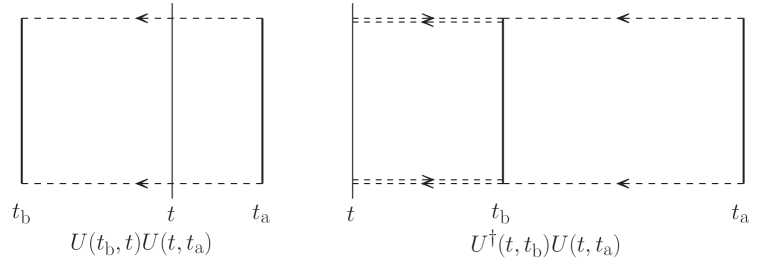
Figure 3: The evolution operator $U(t_{\text{b}},t_{\text{a}})$ is equal to the products shown here. The manifold $\Omega$ is depicted as a vertical segment

7.1 Proof of unitarity – case I

We start from the situation illustrated to the left in fig. 3, which is $t_{\text{a}}<t<t_{\text{b}}$. We first prove (7.2) in the free limit $\mathcal{L}_{I}=0$ and later show that it can be extended to the interacting case.

The identity

$$\langle\bar{z}_{\text{b}},t_{\text{b}};z_{\text{a}},t_{\text{a}}\rangle_{\zeta,\bar{\zeta}}^{\text{free}}=\int\langle\bar{z}_{\text{b}},t_{\text{b}};v,t\rangle_{\zeta,\bar{\zeta}}^{\text{free}}\mathrm{d}\mu_{\bar{v},v}\langle\bar{v},t;z_{\text{a}},t_{\text{a}}\rangle_{\zeta,\bar{\zeta}}^{\text{free}}$$ (7.4)

for $t_{\text{a}}<t<t_{\text{b}}$ easily follows from the formula

$$\int\frac{\omega\mathrm{d}\bar{v}\mathrm{d}v}{i\pi}\mathrm{e}^{-2\omega(\bar{v}v-\bar{a}v-\bar{v}a)}=\mathrm{e}^{2\omega\bar{a}a},$$ (7.5)

upon using the explicit expression (5.25). First, it is obvious that

$$\tilde{W}_{0}(t_{\text{b}},t_{\text{a}})=\tilde{W}_{0}(t_{\text{b}},t)+\tilde{W}_{0}(t,t_{\text{a}}),$$ (7.6)

with self-evident notation. Second, at $\bar{\zeta}^{\prime}=\zeta^{\prime}=0$, we just have the identity

$$\exp(2\bar{z}_{\text{b}}\omega\mathrm{e}^{-i\omega(t_{\text{b}}-t_{\text{a}})}z_{\text{a}})=\mathrm{e}^{2\omega\bar{z}_{0}(t)z_{0}(t)}=\int\mathrm{e}^{2\omega\bar{z}_{0}(t)v}\frac{\omega\mathrm{d}\bar{v}\mathrm{d}v}{i\pi}\mathrm{e}^{-2\omega\bar{v}v}\mathrm{e}^{2\omega\bar{v}z_{0}(t)},$$ (7.7)

which is true by (7.5). Third, at nonvanishing sources $\bar{\zeta}^{\prime}$ and $\zeta^{\prime}$, we have shifts of $a$ and $\bar{a}$ in (7.5), which complete the match. In particular, they provide the correct two-point functions $\langle z(t_{1})\bar{z}(t_{2})\rangle$ for $t_{\text{a}}<t_{1}<t$, $t<t_{2}<t_{\text{b}}$ and $t<t_{1}<t_{\text{b}}$, $t_{\text{a}}<t_{2}<t$.

The interactions can be included by means of formula (5.28), once we observe that the right-hand side of (7.2) can be viewed as the action of the operator

$$\exp\left(i\int_{t}^{t_{\text{b}}}\!\!\mathrm{d}t^{\prime}\!\mathbf{\hskip 0.72229pt}\mathcal{L}_{I}\left(\frac{\delta}{i\delta\bar{\zeta}(t^{\prime})},\frac{\delta}{i\delta\zeta(t^{\prime})}\right)\right)\exp\left(i\int_{t_{\text{a}}}^{t}\!\!\mathrm{d}t\!\mathbf{\hskip 0.72229pt}^{\prime}\mathcal{L}_{I}\left(\frac{\delta}{i\delta\bar{\zeta}(t^{\prime})},\frac{\delta}{i\delta\zeta(t^{\prime})}\right)\right)$$ (7.8)

on the right-hand side of (7.4). The reason why we can move these expressions outside the $\bar{v}$, $v$ integral is that they do not depend on $\bar{v}$ and $v$, as shown by the definition $\mathcal{L}_{I}(z_{\mathbf{n}},\bar{z}_{\mathbf{n}})=L_{I}(\pi_{\mathbf{n}},\varphi_{\mathbf{n}},\phi_{0})$ given right below (5.23): the dependencies on $\bar{v}$ and $v$, $\bar{z}_{0}$ and $z_{0}$ are brought into $\mathcal{L}_{I}$ only after the shift (5.11). Formula (7.8) is just the exponential of the integral between $t_{\text{a}}$ and $t_{\text{b}}$, which is the correct operator that gives the left-hand side of (7.2) by acting on the left-hand side of (7.4), as in (5.28).

Incidentally, we remark that the correct measure $\mathrm{d}\mu_{\bar{v},v}$ can be derived by reversing the procedure just outlined. It is sufficient to work in the free case (7.4), starting from the most general candidate for the measure.

7.2 Useful identities for integrals on coherent states

Before switching to the second part of the proof of unitarity, we derive some useful identities for integrals with coherent states. First note the formulas

$$\int\mathrm{d}\mu_{\bar{v},v}v^{n}\bar{v}^{m}=\frac{n!\delta_{nm}}{(2\omega)^{n}},\qquad\int\frac{\omega\mathrm{d}\bar{\sigma}\mathrm{d}\sigma}{i\pi}\mathrm{e}^{2\omega(\bar{v}-\bar{\sigma})\sigma}g(\bar{\sigma})=g(\bar{v}),$$ (7.9)

where $g$ is an arbitrary function. The first identity is proved by evaluating the integral in polar coordinates $v=\rho\mathrm{e}^{i\theta}$, $\bar{v}=\rho\mathrm{e}^{-i\theta}$, where $\mathrm{d}\mu_{\bar{\sigma},\sigma}=2\omega\rho\mathrm{d}\rho\mathrm{d}\theta/\pi$. The second identity is the delta function representation for coherent states, and follows from the first one by expanding $\mathrm{e}^{2\omega\bar{v}\sigma}g(\bar{\sigma})$ in powers of $\sigma$ and $\bar{\sigma}$.

Moreover, we have

$$\int\frac{\omega\mathrm{d}\bar{v}\mathrm{d}v}{i\pi}\mathrm{e}^{-2\omega(\bar{v}v-\bar{a}v-\bar{v}a)+\varepsilon f(\bar{v},a)-\varepsilon f(\bar{a},v)}=\mathrm{e}^{2\omega\bar{a}a+\mathcal{O}(\varepsilon^{2})},$$ (7.10)

for every function $f$, where $\varepsilon$ is a small parameter. To prove it, it is sufficient to expand the integrand in powers of $\varepsilon$ and check that the first order vanishes by the second formula of (7.9).

7.3 Proof of unitarity – case II

Now we consider the situation illustrated to the right in fig. 3. For $t>t_{\text{b}}$, we have $\langle\bar{z}_{\text{b}},t_{\text{b}};v,t\rangle_{\zeta,\bar{\zeta}}=\langle\bar{v},t;z_{\text{b}},t_{\text{b}}\rangle_{\zeta,\bar{\zeta}}^{\ast}$, from (5.29), so the equation we need to prove reads

$$\langle\bar{z}_{\text{b}},t_{\text{b}};z_{\text{a}},t_{\text{a}}\rangle_{\zeta,\bar{\zeta}}=\int\langle\bar{v},t;z_{\text{b}},t_{\text{b}}\rangle_{\zeta,\bar{\zeta}}^{\ast}\mathrm{d}\mu_{\bar{v},v}\langle\bar{v},t;z_{\text{a}},t_{\text{a}}\rangle_{\zeta,\bar{\zeta}}.$$ (7.11)

Using (7.2), we may write the right-hand side as

$$\int\langle\bar{v},t;z_{\text{b}},t_{\text{b}}\rangle_{\zeta,\bar{\zeta}}^{\ast}\mathrm{d}\mu_{\bar{v},v}\langle\bar{v},t;\sigma,t_{\text{b}}\rangle_{\zeta,\bar{\zeta}}\mathrm{d}\mu_{\bar{\sigma},\sigma}\langle\bar{\sigma},t_{\text{b}};z_{\text{a}},t_{\text{a}}\rangle_{\zeta,\bar{\zeta}}.$$

It is actually sufficient to prove the formula

$$\int\langle\bar{v},t;z_{\text{b}},t_{\text{b}}\rangle_{\zeta,\bar{\zeta}}^{\ast}\mathrm{d}\mu_{\bar{v},v}\langle\bar{v},t;\sigma,t_{\text{b}}\rangle_{\zeta,\bar{\zeta}}=\mathrm{e}^{2\omega\bar{z}_{\text{b}}\sigma},$$ (7.12)

because it turns the right-hand side of (7.11) into

$$\int\frac{\omega\mathrm{d}\bar{\sigma}\mathrm{d}\sigma}{i\pi}\mathrm{e}^{2\omega(\bar{z}_{\text{b}}-\bar{\sigma})\sigma}\langle\bar{\sigma},t_{\text{b}};z_{\text{a}},t_{\text{a}}\rangle_{\zeta,\bar{\zeta}},$$

which is equal to the left-hand side of (7.11) by the second identity of (7.9). Note that formula (7.12) is the unitarity equation (7.3) after a suitable relabeling.

Having reduced the task to proving (7.12), we divide the interval $(t,t_{\text{b}})$ into $n+1$ intervals $(t_{k},t_{k+1})$, $k=0,1,\ldots n$, where $t_{k}=t_{\text{b}}+k\varepsilon$, $\varepsilon=(t-t_{\text{b}})/(n+1)$, and apply (7.2) for every $k$. So doing, we obtain

$$\langle\bar{v},t;\sigma,t_{\text{b}}\rangle_{\zeta,\bar{\zeta}}=\int\left(\prod_{k=1}^{n}\langle\bar{v}_{k+1},t_{k+1};v_{k},t_{k}\rangle_{\zeta,\bar{\zeta}}\mathrm{d}\mu_{\bar{v}_{k},v_{k}}\right)\langle\bar{v}_{1},t_{1};v_{0},t_{0}\rangle_{\zeta,\bar{\zeta}},$$

where $v_{0}=\sigma$, $\bar{v}_{n+1}=\bar{v}$. Doing the same for $\langle\bar{v},t;z_{\text{b}},t_{\text{b}}\rangle_{\zeta,\bar{\zeta}}$ and conjugating, formula (7.12) turns into

$$\int E\left(\prod_{j=1}^{n}\mathrm{d}\mu_{\bar{\sigma}_{j},\sigma_{j}}\langle\bar{\sigma}_{j+1},t_{j+1};\sigma_{j},t_{j}\rangle_{\zeta,\bar{\zeta}}^{\ast}\right)\hskip 1.4457pt\mathrm{d}\mu_{\bar{v},v}\left(\prod_{k=1}^{n}\langle\bar{v}_{k+1},t_{k+1};v_{k},t_{k}\rangle_{\zeta,\bar{\zeta}}\mathrm{d}\mu_{\bar{v}_{k},v_{k}}\right)F=\mathrm{e}^{2\omega\bar{z}_{\text{b}}\sigma},$$ (7.13)

where $\bar{\sigma}_{0}=\bar{z}_{\text{b}}$, $\sigma_{n+1}=v$, $E=\langle\bar{\sigma}_{1},t_{1};\sigma_{0},t_{0}\rangle_{\zeta,\bar{\zeta}}^{\ast}$, $F=\langle\bar{v}_{1},t_{1};v_{0},t_{0}\rangle_{\zeta,\bar{\zeta}}$. We can prove (7.13) for the $n$ we want, since the left-hand side of (7.12) is equal to the left-hand side of (7.13) for every $n$. It is convenient to prove (7.13) in the limit $n\rightarrow\infty$, where $\varepsilon$ becomes infinitesimal. Then we can further reduce the task to the one of proving

$$\int\langle\bar{\sigma}_{j+1},t_{j+1};\sigma_{j},t_{j}\rangle_{\zeta,\bar{\zeta}}^{\ast}\hskip 1.4457pt\mathrm{d}\mu_{\bar{v}_{j+1},\sigma_{j+1}}\langle\bar{v}_{j+1},t_{j+1};v_{j},t_{j}\rangle_{\zeta,\bar{\zeta}}=\mathrm{e}^{2\omega\bar{\sigma}_{j}v_{j}+\mathcal{O}(\varepsilon^{2})}.$$ (7.14)

Indeed, with the help of the relation

$$\int\mathrm{e}^{2\omega\bar{\sigma}_{n}v_{n}}\langle\bar{v}_{n},t_{n};v_{n-1},t_{n-1}\rangle_{\zeta,\bar{\zeta}}\mathrm{d}\mu_{\bar{v}_{n},v_{n}}=\langle\bar{\sigma}_{n},t_{n};v_{n-1},t_{n-1}\rangle_{\zeta,\bar{\zeta}},$$

which follows from the second formula of (7.9), the identity (7.14) for $j=n$ allows us to turn (7.13) into

$$\int\!\!E\!\left(\prod_{j=1}^{n-1}\mathrm{d}\mu_{\bar{\sigma}_{j},\sigma_{j}}\langle\bar{\sigma}_{j+1},t_{j+1};\sigma_{j},t_{j}\rangle_{\zeta,\bar{\zeta}}^{\ast}\!\right)\!\mathrm{d}\mu_{\bar{v},v}\!\!\left(\prod_{k=1}^{n-1}\langle\bar{v}_{k+1},t_{k+1};v_{k},t_{k}\rangle_{\zeta,\bar{\zeta}}\mathrm{d}\mu_{\bar{v}_{k},v_{k}}\!\right)\!F=\mathrm{e}^{2\omega\bar{z}_{\text{b}}\sigma+\mathcal{O}(\varepsilon^{2})},$$

with $\bar{v}_{n}=\bar{\sigma}_{n}=\bar{v}$, $\sigma_{n}=v$, which is the same as (7.13) with $n\rightarrow n-1$, $t\rightarrow t_{n}$, up to $\mathcal{O}(\varepsilon^{2})$ in the exponent. Iterating in $n$, the last step is (7.14) with $j=0$. Taking $\varepsilon$ to zero, (7.13) follows for $n\rightarrow\infty$, as desired.

It remains to prove (7.14) for infinitesimal $\varepsilon$, which is relatively easy. Using (5.28) and (5.25), we have

$$\langle\bar{v}_{j+1},t_{j+1};v_{j},t_{j}\rangle_{\zeta,\bar{\zeta}}=\mathrm{e}^{i\tilde{W}_{0j}+2\bar{v}_{j+1}\omega(1\!-i\omega\varepsilon)v_{j}+i\varepsilon\mathbf{\hskip 0.72229pt(}\bar{\zeta}_{j}^{\prime}v_{j}+\bar{v}_{j+1}\zeta_{j}^{\prime})+i\varepsilon\mathbf{\hskip 0.72229pt}\mathcal{L}_{I}(v_{j},\bar{v}_{j+1})+\mathcal{O}(\varepsilon^{2})},$$

where $\tilde{W}_{0j}$, $\bar{\zeta}_{j}^{\prime}$ and $\zeta_{j}^{\prime}$ are the restrictions of $\tilde{W}_{0}$, $\bar{\zeta}^{\prime}$ and $\zeta^{\prime}$ to the $(j+1)$-th interval. We see that (7.14) is just a particular case of formula (7.10), with $\bar{a}=\bar{\sigma}_{j}$, $a=v_{j}$, $\bar{v}=\bar{v}_{j+1}$, $v=\sigma_{j+1}$ (recalling that the Lagrangian is assumed to the Hermitian). This concludes the proof.

Equation (7.11) turns into the unitarity equation $S^{{\dagger}}S=1$ obeyed by the $S$ matrix when $t\rightarrow+\infty$, $t_{\text{b}}\rightarrow-\infty$, $t_{\text{a}}\rightarrow-\infty$, $\tau\rightarrow 0$. Indeed, the left-hand side is equal to $\mathrm{e}^{2\omega\bar{z}_{\text{b}}z_{\text{a}}}$ for $\tau=0$, which is the matrix element of the identity matrix in the coherent-state approach.

8 Unitarity equations

In this section we work out the diagrammatic versions of the unitarity equation, which are also known as Cutkosky-Veltman identities [4]. To this purpose, it is useful to define the cut correlation functions

$$\langle\tilde{z}(t_{1})\cdots\tilde{z}(t_{k})\hskip 0.72229pt|\hskip 0.72229pt\tilde{z}(t_{k+1})\cdots\tilde{z}(t_{k+n})\rangle_{\zeta,\bar{\zeta}}\equiv\!\!\int\!\!\frac{\delta^{k}\langle\bar{v},t;z_{\text{b}},t_{\text{b}}\rangle_{\zeta,\bar{\zeta}}^{\ast}}{i\delta\tilde{\zeta}(t_{1})\cdots i\delta\tilde{\zeta}(t_{k})}\mathrm{d}\mu_{\bar{v},v}\frac{\delta^{n}\langle\bar{v},t;z_{\text{a}},t_{\text{a}}\rangle_{\zeta,\bar{\zeta}}}{i\delta\tilde{\zeta}(t_{k+1})\cdots i\delta\tilde{\zeta}(t_{k+n})}\!\!\!,$$ (8.1)

where $\tilde{z}(t_{j})$ and $\tilde{\zeta}(t_{j})$ stand for $z(t_{j})$ and $\bar{\zeta}(t_{j})$, or $\bar{z}(t_{j})$ and $\zeta(t_{j})$, depending on the case. We choose to write formula (8.1) in the form that is more convenient for $t>t_{\text{b}}$, since the simpler case $t<t_{\text{b}}$ can be easily reached by means of formula (5.29), i.e., by understanding $\langle\bar{v},t;z_{\text{b}},t_{\text{b}}\rangle_{\zeta,\bar{\zeta}}^{\ast}$ as $\langle\bar{z}_{\text{b}},t_{\text{b}};v,t\rangle_{\zeta,\bar{\zeta}}$. Strictly speaking, we should set $\zeta=\bar{\zeta}=0$ at the end, but it is not really necessary to do so for the validity of the identities that we are going to study. It is understood that the correlation functions we write vanish when an insertion $\tilde{z}(t_{j})$ lies outside the right time interval, which is identified by the functional differentiation it originates from. In (8.1), we have zero when $t_{j}\notin(t_{\text{b}},t)$ for $j\leqslant k$, or $t_{j}\notin(t_{\text{a}},t)$ for $j\geqslant k$.

The correlation functions (8.1) are made of two parts, identified by two sets of insertions, which stand on the opposite sides of what we may call a “cut”, denoted by the vertical bar. The diagrams contributing to (8.1) are called “cut diagrams”. In fig. 4 we list the cut diagrams associated with the last diagram of fig. 1.

Similarly, we can define cut correlation functions that contain insertions of composite fields. Cut correlation functions with insertions of $w$ and $\bar{w}$ follow from the change of variables (4.12), or (5.11).

An important remark is that the correlation functions

$$\langle\hskip 0.72229pt|\hskip 0.72229pt\tilde{z}(t_{1})\cdots\tilde{z}(t_{n})\rangle_{\zeta,\bar{\zeta}},\qquad\langle\tilde{z}(t_{1})\cdots\tilde{z}(t_{n})\hskip 0.72229pt|\hskip 0.72229pt\rangle_{\zeta,\bar{\zeta}},\qquad\langle\tilde{z}(t_{1})\cdots\tilde{z}(t_{n})\rangle_{\zeta,\bar{\zeta}},$$ (8.2)

do not coincide at finite $\tau$ on a compact $\Omega$. The first two are cut correlation functions where all the external legs are located on the same side with respect to the cut. The third one is the correlation function defined in (5.30) (omitting $\bar{z}_{\text{b}},t_{\text{b}}$ and $\hskip 0.72229ptz_{\text{a}},t_{\text{a}}$, for simplicity, and keeping arbitrary sources $\zeta$, $\bar{\zeta}$), which has no cut. Recall that every vertex is attached to an external source $K$, which takes care of the restriction to finite $\tau$ and compact $\Omega$. We show below that every propagator that crosses a cut (called “cut propagator”) flows (positive) energy towards the same side of the cut (as occurs at $\tau=\infty$, $\Omega=\mathbb{R}^{3}$). We know, however, that there is no energy conservation at the vertices, because a source $K$ can flow energy in or out. For example, a vertex can be cut out of a diagram and still contribute: the left diagram of fig. 4 is nontrivial, because energy may flow in and out through the upper source $K$. Diagrams like these make the difference between the third correlation function of (8.2) and the other two.

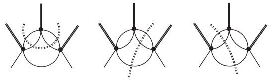
Figure 4: Cut diagrams associated with the last diagram of fig. 1. The cut is denoted by a dashed double line

Now we show how to use the cut correlation functions to express unitarity diagrammatically, by means of the cut diagrams. Differentiating (7.11), we obtain the identities

$$\frac{\delta^{n}\int\langle\bar{v},t;z_{\text{b}},t_{\text{b}}\rangle_{\zeta,\bar{\zeta}}^{\ast}\mathrm{d}\mu_{\bar{v},v}\langle\bar{v},t;z_{\text{a}},t_{\text{a}}\rangle_{\zeta,\bar{\zeta}}}{i\delta\tilde{\zeta}(t_{1})\cdots i\delta\tilde{\zeta}(t_{n})}=\frac{\delta^{n}\langle\bar{z}_{\text{b}},t_{\text{b}};z_{\text{a}},t_{\text{a}}\rangle_{\zeta,\bar{\zeta}}}{i\delta\tilde{\zeta}(t_{1})\cdots i\delta\tilde{\zeta}(t_{n})}\equiv\langle\tilde{z}(t_{1})\cdots\tilde{z}(t_{n})\rangle_{\zeta,\bar{\zeta}},\qquad$$ (8.3)

for every $n\geqslant 0$. Using the Leibniz rule on the left-hand side, we obtain the Cutkosky-Veltman equation obeyed by the $n$-point function, which reads

$$\sum_{k=0}^{n}\sum_{\pi_{k}}(-1)^{k}\langle\tilde{z}(t_{\pi(1)})\cdots\tilde{z}(t_{\pi(k)})\hskip 0.72229pt|\hskip 0.72229pt\tilde{z}(t_{\pi(k+1)})\cdots\tilde{z}(t_{\pi(k+n)})\rangle_{\zeta,\bar{\zeta}}=\langle\tilde{z}(t_{1})\cdots\tilde{z}(t_{n})\rangle_{\zeta,\bar{\zeta}},$$ (8.4)

where $\pi_{k}$ denotes the set of $k$-combinations $(\pi(1),\ldots,\pi(k))$ of the set $(1,\ldots,n)$.

The identities (8.4) are particularly interesting for $t>t_{\text{b}}$, which is the case of the unitarity equation (7.1). When $t_{j}>t_{\text{b}}$ for some $j$ the right-hand sides of (8.3) and (8.4) vanish.

Now we explain how to build diagrams for the cut correlation functions (8.1) and the identities (8.4). Each side of the cut is built as explained in section 5, so we can concentrate on the cut itself, which is given by the integral on $v$ and $\bar{v}$. The left-hand side of the cut depends on $v$, while the right-hand side depends on $\bar{v}$. Formulas (5.25), (5.27) and (5.28) show that, if we treat the interaction Lagrangian $\mathcal{L}_{I}$ as in (5.28), the dependence on $v$ and $\bar{v}$ stems from the free generating functional $W^{\text{free}}$ (which is at most linear in $v$, or $\bar{v}$, on each side of the cut), and spreads around due to the functional derivatives contained in $\mathcal{L}_{I}$.

We expand in powers of $v$ to the left of the cut, and in powers of $\bar{v}$ to the right of the cut. Then, the integration measure $\mathrm{d}\mu_{\bar{v},v}$ makes the $v$-$\bar{v}$ integrals convergent. Every $v$-$\bar{v}$ integral we obtain can be evaluated with the help of the first identity of (7.9), which can be viewed as Wick’s theorem for $v$ and $\bar{v}$. Indeed, $1/(2\omega)$ is the “elementary” $v$-$\bar{v}$ cut propagator, and the factor $n!$ takes care of all the possibilities of associating a $v$ to some $\bar{v}$. In the end, the two sides of the cut are connected by the $v$-$\bar{v}$ integrals.

It is convenient to introduce different sources $\zeta,\bar{\zeta}$ for $\langle\bar{v},t;z_{\text{b}},t_{\text{b}}\rangle_{\zeta,\bar{\zeta}}^{\ast}$ and $\langle\bar{v},t;z_{\text{a}},t_{\text{a}}\rangle_{\zeta,\bar{\zeta}}$ in (8.3). We denote them by means of subscripts $-$ and $+$, respectively. Then (8.3) can be written as

$$\left.\mathcal{D}_{n}^{-+}\int\langle\bar{v},t;z_{\text{b}},t_{\text{b}}\rangle_{\zeta_{-},\bar{\zeta}_{-}}^{\ast}\mathrm{d}\mu_{\bar{v},v}\langle\bar{v},t;z_{\text{a}},t_{\text{a}}\rangle_{\zeta_{+},\bar{\zeta}_{+}}\right|_{+=-}=\langle\tilde{z}(t_{1})\cdots\tilde{z}(t_{n})\rangle_{\zeta,\bar{\zeta}},$$ (8.5)

where

$$\mathcal{D}_{n}^{-+}\equiv\prod_{j=1}^{n}\left(\frac{\delta}{i\delta\tilde{\zeta}_{-}(t_{j})}+\frac{\delta}{i\delta\tilde{\zeta}_{+}(t_{j})}\right)$$

and “$+=-$” stands for $\zeta_{+}=\zeta_{-}=\zeta$, $\bar{\zeta}_{+}=\bar{\zeta}_{-}=\bar{\zeta}$. Separating the interactions $\mathcal{L}_{I}$ from the rest by means of (5.28), we also have

$$\left.\mathcal{D}_{n}^{-+}\mathcal{D}_{I}^{-\ast}\mathcal{D}_{I}^{+}\int\langle\bar{v},t;z_{\text{b}},t_{\text{b}}\rangle_{\zeta_{-},\bar{\zeta}_{-}}^{\text{free}\ast}\mathrm{d}\mu_{\bar{v},v}\langle\bar{v},t;z_{\text{a}},t_{\text{a}}\rangle_{\zeta_{+},\bar{\zeta}_{+}}^{\text{free}}\right|_{+=-}=\langle\tilde{z}(t_{1})\cdots\tilde{z}(t_{n})\rangle_{\zeta,\bar{\zeta}},$$ (8.6)

where

$$\mathcal{D}_{I}^{\pm}\equiv\exp\left(i\int_{t_{\pm}}^{t}\!\!\mathrm{d}t^{\prime}\!\mathbf{\hskip 0.72229pt}\mathcal{L}_{I}\left(\frac{\delta}{i\delta\bar{\zeta}_{\pm}(t^{\prime})},\frac{\delta}{i\delta\zeta_{\pm}(t^{\prime})}\right)\right).$$

$t_{+}$ standing for $t_{\text{a}}$, and $t_{-}$ standing for $t_{\text{b}}$. As explained after (7.8), we can move these expressions outside the $\bar{v}$, $v$ integral, because $\mathcal{L}_{I}$ does not depend on $\bar{v}$ and $v$ before the shift (5.11). Formula (8.6) shows that it is sufficient to calculate

$$\mathrm{e}^{iW_{-+}^{\text{free}}}\equiv\int\langle\bar{v},t;z_{\text{b}},t_{\text{b}}\rangle_{\zeta_{-},\bar{\zeta}_{-}}^{\text{free}\ast}\mathrm{d}\mu_{\bar{v},v}\langle\bar{v},t;z_{\text{a}},t_{\text{a}}\rangle_{\zeta_{+},\bar{\zeta}_{+}}^{\text{free}},$$ (8.7)

since everything else follows from it by means of repeated functional differentiations. The calculation is straightforward. Basically, we have already done it earlier to prove (7.4). The result is

$$iW_{-+}^{\text{free}}=i \tilde{W}_{0}+2\omega\bar{z}_{0}(t)z_{0}(t)+\int_{t_{\text{b}}}^{t}\mathrm{d}t^{\prime}\int_{t_{\text{a}}}^{t}\mathrm{d}t^{\prime\prime}\bar{\zeta}_{-}^{\prime}(t^{\prime})\frac{\mathrm{e}^{-i\omega(t^{\prime}-t^{\prime\prime})}}{2\omega}\zeta_{+}^{\prime}(t^{\prime\prime})$$ (8.8)

$$-i\int_{t_{\text{b}}}^{t}\mathrm{d}t^{\prime}\hskip 0.72229pt\left.\mathbf{(}\bar{\zeta}_{-}^{\prime}z_{0}+\bar{z}_{0}\zeta_{-}^{\prime})\right|_{t^{\prime}}-\int_{t_{\text{b}}}^{t}\mathrm{d}t^{\prime}\int_{t_{\text{b}}}^{t}\mathrm{d}t^{\prime\prime}\bar{\zeta}_{-}^{\prime}(t^{\prime})\theta(t^{\prime\prime}-t^{\prime})\frac{\mathrm{e}^{-i\omega(t^{\prime}-t^{\prime\prime})}}{2\omega}\zeta_{-}^{\prime}(t^{\prime\prime})$$

$$+i\int_{t_{\text{a}}}^{t}\mathrm{d}t^{\prime}\hskip 0.72229pt\left.\mathbf{(}\bar{\zeta}_{+}^{\prime}z_{0}+\bar{z}_{0}\zeta_{+}^{\prime})\right|_{t^{\prime}}-\int_{t_{\text{a}}}^{t}\mathrm{d}t^{\prime}\int_{t_{\text{a}}}^{t}\mathrm{d}t^{\prime\prime}\bar{\zeta}_{+}^{\prime}(t^{\prime})\theta(t^{\prime}-t^{\prime\prime})\frac{\mathrm{e}^{-i\omega(t^{\prime}-t^{\prime\prime})}}{2\omega}\zeta_{+}^{\prime}(t^{\prime\prime}),\qquad$$

where $\tilde{W}_{0}$ is the same as in (5.27), the functions $\bar{z}_{0}(t)$ and $z_{0}(t)$ are the same as in (4.13), while $\zeta_{\pm}^{\prime}=\zeta_{\pm}+A+i\omega B$, $\bar{\zeta}_{\pm}^{\prime}=\bar{\zeta}_{\pm}+A-iB\omega$, as in (5.26).

Now we explain the meanings of the various terms that appear in (8.8). The double integral in the last line encodes the usual propagator (4.18)-(5.16), which connects vertices placed to the right of the cut. The double integral in the second line encodes the conjugate propagator, which connects vertices placed to the left of the cut. The double integral in the first line encodes the cut propagator, which connects vertices located on opposite sides of the cut.

Differentiating with respect to $\bar{\zeta}_{-}(t_{1})$ and $\zeta_{+}(t_{2})$, and concentrating on the connected part of the two-point function (denoted by the subscript $c$), we find

$$\langle z(t_{1})\hskip 0.72229pt|\hskip 0.72229pt\bar{z}(t_{2})\rangle_{c}^{\text{free}}=\frac{\mathrm{e}^{-i\omega(t_{1}-t_{2})}}{2\omega},\qquad\langle z(e)\hskip 0.72229pt|\hskip 0.72229pt\bar{z}(-e)\rangle_{c}^{\text{free}}=(2\pi)\theta(e)\delta(e^{2}-\omega^{2}),$$ (8.9)

before and after the Fourier transform. Differentiating with respect to $\bar{\zeta}_{+}(t_{1})$ and $\zeta_{-}(t_{2})$, we find $\langle\bar{z}(t_{1})\hskip 0.72229pt|\hskip 0.72229ptz(t_{2})\rangle_{c}^{\text{free}}=0$, instead. This proves that positive energies flow through the cut in a unique direction (from the right to the left).

Note that $W_{-+}^{\text{free}}$ includes several contributions that are linear in $\zeta^{\pm}\$and $\bar{\zeta}^{\pm}$. When the functional derivatives act on those, the legs associated with them do not connect vertices, but end into external sources (endpoints), built with $\phi_{0}$, $z_{0}$ and $\bar{z}_{0}$, which carry information about the restrictions to finite $\tau$ and finite volume.

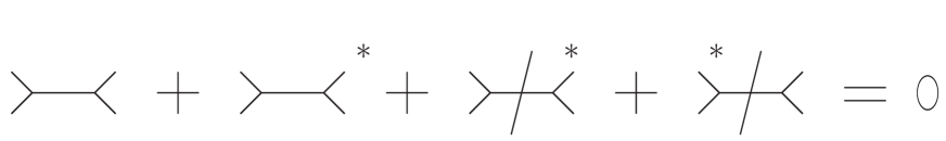
Figure 5: Cutkosky-Veltman identity for the propagator

The result confirms that the cut propagators (8.9) know nothing about the restriction to finite times (and little enough about the restriction to finite volume, which amounts to the discretization of the frequencies $\omega$), like the (uncut) propagators (5.16). This property ensures that the spectral optical identities expressing unitarity coincide with the usual ones, internally (apart from the discretization of the loop momenta), and differ only externally. Details on this are given in the next section, where we use them to introduce purely virtual particles at finite $\tau$ on a compact $\Omega$.

The simplest examples of equations (8.4) are those of the one- and two-point functions. Formula (8.3) with $n=1$, $t>t_{1}>t_{\text{b}}$, gives

$$\langle z(t_{1})\hskip 0.72229pt|\hskip 0.72229pt\rangle=\langle\hskip 0.72229pt|\hskip 0.72229ptz(t_{1})\rangle,\qquad\langle\bar{z}(t_{1})\hskip 0.72229pt|\hskip 0.72229pt\rangle=\langle\hskip 0.72229pt|\hskip 0.72229pt\bar{z}(t_{1})\rangle.$$ (8.10)

In the free limit $\mathcal{L}_{I}\rightarrow 0$, we find

$$\mathrm{e}^{-iW_{-+}^{\text{free\hskip 0.72229pt0}}}\langle z(t_{1})\hskip 0.72229pt|\hskip 0.72229pt\rangle^{\text{free}}=\left.\frac{\mathrm{e}^{-iW_{-+}^{\text{free}}}\delta\mathrm{e}^{iW_{-+}^{\text{free}}}}{-i\delta\bar{\zeta}_{-}(t_{1})}\right|_{\zeta_{\pm}=\bar{\zeta}_{\pm}=0}\!\!\!\!\!\!\!\!\!\!\!\!\!=z_{0}(t_{1})+i\!\int_{t_{\text{a}}}^{t}\!\!\mathrm{d}t^{\prime}\theta(t_{1}-t^{\prime})\frac{\mathrm{e}^{-i\omega(t_{1}-t^{\prime})}}{2\omega}\left.(A+i\omega B)\right|_{t^{\prime}},$$ (8.11)

where $W_{-+}^{\text{free\hskip 0.72229pt0}}\equiv\left.W_{-+}^{\text{free}}\right|_{\zeta_{\pm}=\bar{\zeta}_{\pm}=0}$. The same result is obtained for $\langle\hskip 0.72229pt|\hskip 0.72229ptz(t_{1})\rangle^{\text{free}}$, which is calculated as $-i\delta\mathrm{e}^{iW_{-+}^{\text{free}}}/\delta\bar{\zeta}_{+}(t_{1})$. The second identity of (8.10) is verified similarly at $\mathcal{L}_{I}=0$. For $t_{1}<t_{\text{b}}$, we have $\langle\hskip 0.72229pt|\hskip 0.72229ptz(t_{1})\rangle=\langle z(t_{1})\rangle$, $\langle\hskip 0.72229pt|\hskip 0.72229pt\bar{z}(t_{1})\rangle=\langle\bar{z}(t_{1})\rangle$, which are trivial in the free limit.

Formula (8.4) for $n=2$, $\tilde{z}(t_{1})=z(t_{1})$, $\hskip 0.72229pt\tilde{z}(t_{2})=\bar{z}(t_{2})$, gives

$$\langle\hskip 0.72229pt|z(t_{1})\bar{z}(t_{2})\hskip 0.72229pt\rangle-\langle z(t_{1})\hskip 0.72229pt|\hskip 0.72229pt\bar{z}(t_{2})\rangle-\langle\bar{z}(t_{2})\hskip 0.72229pt|\hskip 0.72229ptz(t_{1})\rangle+\langle z(t_{1})\bar{z}(t_{2})\hskip 0.72229pt|\hskip 0.72229pt\rangle=\langle z(t_{1})\bar{z}(t_{2})\rangle.$$

In the free limit, the connected components give

$$\theta(t_{1}-t_{2})\frac{\mathrm{e}^{-i\omega(t_{1}-t_{2})}}{2\omega}\qquad-\frac{\mathrm{e}^{-i\omega(t_{1}-t_{2})}}{2\omega}\qquad-0\qquad+\theta(t_{2}-t_{1})\frac{\mathrm{e}^{-i\omega(t_{1}-t_{2})}}{2\omega}\qquad=0,$$

for $t>t_{1,2}>t_{\text{b}}$, after simplifying the common normalization factor $\mathrm{e}^{iW_{-+}^{\text{free\hskip 0.72229pt0}}}$. This identity is illustrated in fig. 5. For $t_{\text{b}}>t_{1,2}$, $t_{1}>t_{\text{b}}>t_{2}$ and $t_{2}>t_{\text{b}}>t_{1}$, we have $\langle\hskip 0.72229pt|z(t_{1})\bar{z}(t_{2})\hskip 0.72229pt\rangle=\langle z(t_{1})\bar{z}(t_{2})\rangle$, $\langle\hskip 0.72229pt|z(t_{1})\bar{z}(t_{2})\hskip 0.72229pt\rangle=\langle z(t_{1})\hskip 0.72229pt|\hskip 0.72229pt\bar{z}(t_{2})\rangle$ and $\langle\hskip 0.72229pt|z(t_{1})\bar{z}(t_{2})\hskip 0.72229pt\rangle=\langle\bar{z}(t_{2})\hskip 0.72229pt|\hskip 0.72229ptz(t_{1})\rangle$, respectively, which are also trivial in the free limit.

The unitarity equations (7.3) and (7.12) are studied by assuming $t>t_{\text{b}}=t_{\text{a}}$ in (8.3). Then the right-hand sides of (8.3) and (8.4) vanish for every $n>0$. Separating the uncut diagram $G$ (and its conjugate diagram $G^{\ast}$) from every other contributions to the left-hand side, equation (8.4) can be written in the usual form, which is

$$G+G^{\ast}+\sum_{c}G_{c}=0,$$ (8.12)

where the sum is on all the diagrams that contain nontrivial cuts, including those coming from the first two correlation functions of (8.2). The minus signs of (8.4) are included into the definitions of cut diagrams. We illustrate the equation in fig. 6.

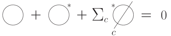
Figure 6: Diagrammatic unitarity equations

The diagrammatic rules for the identities (8.12) are as follows.

— Draw a vertical bar, which denotes the cut.

— Distribute the external legs in all possible ways on the two sides, with a minus sign for each leg to the left.

— Do the same for the vertices and the endpoints (“one-leg vertices”) that contribute to the order you are interested in.

— Draw the diagrams by connecting (internal and external) legs to vertices and endpoints in all possible ways.

— Two legs $z$, $\bar{z}$ are connected to each other by means of ordinary propagators (when they both lie to the right of the cut), conjugate propagators (when they both lie to the left), or cut propagators (when they lie on opposite sides).

Ultimately, formulas (8.12), and the rules just stated, are the same as usual. The only differences are that: $i$) the loop momenta are discretized; $ii$) each vertex has an external source $K$ attached to it; $iii$) there are endpoints, due to the restrictions to finite $\tau$ and compact $\Omega$. Endpoints are actually common at $\tau=\infty$, $\Omega=\mathbb{R}^{3}$ as well (for example, when the field is shifted by a nontrivial background).

In fig. 7 we show examples of cut diagrams with two cubic vertices. Note that the cut may also cross legs attached to endpoints. This is because the endpoints (8.11) receive contributions from both sides of the cut.

As said, the identities (8.12) encode the unitarity equation (7.1), which is also (7.3), (7.12), or the cases $t>t_{\text{b}}=t_{\text{a}}$ of (7.11) and (8.3). When we relax these restrictions, we have other diagrammatic identities, which encode the more general equation (1.1). They look similar to (8.12), but for the following differences. First, the right-hand side needs not be zero: it is replaced by the diagrammatic version of the right-hand side of (8.4). In addition, when $t_{\text{b}}>t$, no minus signs are attached to the legs and the vertices located to the left of the cut, the conjugate propagators are replaced by (unconjugate) propagators and the cut propagators across the cut coincide with the same (uncut) propagators.

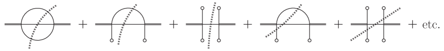
Figure 7: Cut diagrams with two vertices

9 Purely virtual particles

In this section we introduce purely virtual particles at finite $\tau$ on a compact space manifold $\Omega$, after briefly recalling what they are at $\tau=\infty$, $\Omega=\mathbb{R}^{3}$, and how they are introduced there, following [2]. For the time being, we assume that all the particles have kinetic terms with the correct signs, and explain how to render some physical particles purely virtual. Later, we explain how to render ghosts purely virtual as well. We recall that tachyons cannot be rendered purely virtual.

Consider an arbitrary Feynman diagram $G$ in momentum space, where, by assumption, the propagators are defined by means of the usual $i\epsilon$ prescription. Label each internal leg by means of an index $a,b,\ldots$. Let $m_{a}$ denote the mass of the $a$-th leg, and $k^{\mu}-p_{a}^{\mu}$ its four-momentum. Here $k^{\mu}=(k^{0},\mathbf{k})$ denotes a loop four-momentum, or a combination of loop four-momenta, while $p_{a}^{\mu}=(e_{a},\mathbf{p}_{a})$ is an external four-momentum. The frequency of the $a$-th leg is $\omega_{a}=\sqrt{m_{a}^{2}+(\mathbf{k}-\mathbf{p}_{a})^{2}}$. Note that each internal leg is equipped with its own $p_{a}^{\mu}$. This redundant notation (various $p_{a}^{\mu}$ may depend on one another) makes the formulas more symmetric and easier to handle.

We integrate on the loop energies $k^{0}$ with measure $\mathrm{d}k^{0}/(2\pi)$, by means of the residue theorem, and completely ignore the integrals on the loop momenta $\mathbf{k}$. The reason is that the identities we derive, which are crucial to switch to purely virtual particles, hold for arbitrary values of the frequencies $\omega_{a}$.

After integrating on the loop energies, we rearrange the results in order to remove the differences of frequencies from the denominators. We remain with denominators of the form

$$\frac{1}{E-\sum_{i}\omega_{a_{i}}+i\epsilon},$$

where $E$ is a linear combination of external energies. At this point, we make the “threshold decomposition”, to separate the on-shell contributions from the off-shell ones, by carefully applying the identity

$$\frac{i}{x+i\epsilon}=\mathcal{P}\frac{i}{x}+\pi\delta(x),$$ (9.1)

where $\mathcal{P}$ denotes the Cauchy principal value. The number of delta functions is called “level” of the threshold decomposition.

What just said applies to the diagrams that contain ordinary, physical particles, which we denote by $G_{\text{ph}}$. A certain surgical operation on $G_{\text{ph}}$ allows us to define new diagrams $G_{\text{pv}}$, where some internal legs are purely virtual. This is achieved by removing all the on shell contributions that involve the particles we want to render purely virtual. Let $\omega_{\text{pv}}$ denote the frequencies of those particles in $G_{\text{ph}}$. Given the threshold decomposition of $G_{\text{ph}}$, the threshold decomposition of $G_{\text{pv}}$ is obtained by dropping every contribution that involves delta functions with $\omega_{\text{pv}}$-dependent supports. Finally, $G_{\text{pv}}$ itself is defined from its own threshold decomposition.

At the tree level, the $w$-$\bar{w}$ propagator of formula (5.16) loses the delta function and becomes a principal value:

$$\langle w(e)\bar{w}(-e)\rangle_{c}^{\text{free}}\rightarrow\mathcal{P}\frac{i}{2\omega(e-\omega)},\qquad\langle w(t)\hskip 0.72229pt\bar{w}(t^{\prime})\rangle_{c}^{\text{free}}\rightarrow\text{sgn}(t-t^{\prime})\frac{\mathrm{e}^{-i\omega(t-t^{\prime})}}{4\omega},$$ (9.2)

where sgn$(t)=\theta(t)-\theta(-t)$ is the sign function.

In a one-loop diagram, the identity (9.1) separates quantities such as

$$\mathcal{P}^{ab}\equiv\mathcal{P}\frac{1}{e_{a}-e_{b}-\omega_{a}-\omega_{b}},\qquad\Delta^{ab}\equiv\pi\delta(e_{a}-e_{b}-\omega_{a}-\omega_{b}).$$

Once the threshold decomposition is completed, we remove all the contributions that contain a $\Delta^{ab}$ where $\omega_{a}$, or $\omega_{b}$, or both, are the frequencies of particles that we want to render purely virtual. In diagrams with more loops similar rules apply. Sums of more than two frequencies may appear in the supports of the delta functions.

For example, the usual bubble diagram gives a result proportional to

$$\frac{i}{e_{1}-e_{2}-\omega_{1}-\omega_{2}+i\epsilon}+\frac{i}{e_{2}-e_{1}-\omega_{1}-\omega_{2}+i\epsilon},$$ (9.3)

after integrating on the loop energy. If we want to render the particles propagating in one or two internal legs purely virtual, we replace the result by $i$ times

$$\mathcal{P}^{12}+\mathcal{P}^{21},$$ (9.4)

by dropping the contributions $\Delta^{12}$ and $\Delta^{21}$. For details of the triangle, the box, etc., and diagrams with more loops, see [2, 1].

The prescription just recalled takes care of the internal sectors of the diagrams. For consistency, we must also restrict the external sectors, by demanding that only physical particles lie on the external legs. So doing, we project the set of states to the physical subspace. The physical amplitudes are the amplitudes between incoming and outgoing physical particles. Any other amplitude is dropped because unphysical.

The combination made by this projection and the prescription described above defines a map $M_{\text{pv}}$ from a starting theory to a new theory. The starting theory contains physical particles (and possibly ghosts). The final theory contains physical particles and purely virtual particles.

The map $M_{\text{pv}}$ is consistent with unitarity as follows: $i$) if the starting theory is unitary (i.e., it has no ghosts), the final theory is unitary; $ii$) if the starting theory has ghosts, the final theory is unitary, provided all the ghosts are turned into purely virtual particles. In other words, if we convert a subset of physical particles (and all the ghosts, if present) into purely virtual particles, we preserve (or gain) unitarity.

The reason why unitarity is preserved, or gained, relies on an important fact: that the thresholds are independent from one another, so the unitarity equations (8.12) split into a large number of independent “spectral optical identities” [2], one for each threshold, which hold algebraically, before integrating on the loop momenta. Suppressing certain types of thresholds everywhere, the identities (8.12) remain true. Moreover, the cut diagrams where a cut crosses one or more legs of purely virtual particles disappear entirely, because the cut propagators associated with those legs are delta functions with $\omega_{\text{pv}}$-dependent supports. This is consistent with projecting the purely virtual particles away externally.

In the case of theories with physical particles only (no ghosts), the Cutkosky-Veltman identities (8.12) encode the unitarity of the starting theory. After implementing the prescription/projection to purely virtual particles, they encode the unitarity of the final theory. In the presence of ghosts, instead, the identities (8.12) do not express unitarity, since the starting theory is not unitary. Yet, they are still valid (they are called pseudounitarity equations), and very useful. What is important is that, after the prescription/projection, they encode the unitarity of the final theory, provided all the ghosts are rendered purely virtual.

It is important to stress that the diagrammatics of purely virtual particles is not governed by time ordering [1], so the map $M_{\text{pv}}$ does not commute with the diagrammatic rules: it acts on the amplitudes and the diagrams as such. More precisely, a loop diagram containing purely virtual particles cannot be built by using the projected propagators of (9.8) inside an ordinary diagram: it should be built by projecting the ordinary diagram as a whole. An explicit example can clarify this point. We know that the tree propagator (5.16) is mapped into (9.2), and the ordinary bubble diagram (9.3) is mapped into (9.4). However, if we build a bubble diagram with two propagators (9.2), we do not obtain (9.4): we obtain something that is very different, and not even consistent with unitarity (see [25]). For the same reason, simple separations between the free and interaction parts, such as those encoded in formulas (4.20), (5.28) and (8.6), do not commute with the map $M_{\text{pv}}$ (beyond the tree level).

The extension to purely virtual particles is an interesting option that was overlooked before. Nevertheless, it is allowed by quantum field theory, and might be the solution to the problem of quantum gravity [8, 12].

9.1 Purely virtual particles in a finite interval of time and on a compact manifold

What we have just said holds at $\tau=\infty$, $\Omega=\mathbb{R}^{3}$. We can generalize it to finite $\tau$ and compact $\Omega$ as follows.

A purely virtual particle is not associated with a dynamical degree of freedom, since its on shell contributions are removed from the physical quantities. In this respect, it is a sort of fake particle. Consequently, it cannot have nontrivial initial or final conditions. This means that, at finite $\tau$, on a compact $\Omega$, the projection to purely virtual particles mentioned earlier is the set of conditions

$$z(t_{\text{i}})=\bar{z}(t_{\text{f}})=0.$$ (9.5)

The particles we want to render purely virtual are thereby removed from the external sectors of the diagrams.

As far as the boundary conditions are concerned, we can keep them in the general form (5.1), since they are not associated with degrees of freedom. For example, the integral in between the right-hand side of (7.2) does not concern them. Besides, the function $f(t,\mathbf{x}_{\partial\Omega})$ might describe some property of our experimental apparatus.

Next, we have to free the interior parts of the diagrams from the on shell contributions due to the particles that we want to render purely virtual. This goal can be achieved exactly as before, since the internal parts of the diagrams are basically the same as at $\tau=\infty$, $\Omega=\mathbb{R}^{3}$.

Let us recapitulate what we know. We have shown that quantum field theory (with physical particles and possibly ghosts) can be formulated diagrammatically at finite $\tau$ and on a compact space manifold $\Omega$. The diagrams are the same as usual, internally, apart from a non invasive change, which is the discretization of the loop momenta. Every other detail about the restriction to finite $\tau$ and compact $\Omega$ is moved away to the external sources $K$ (by which we also mean the endpoints). We have seen that the Cutkovsky-Veltman identities (8.12) are the same as usual, apart from the external sources and the discretization of the loop momenta. They encode the unitarity or pseudounitarity equation (7.1) of the starting theory (depending on whether ghosts are absent or present).

We also know that at $\tau=\infty$, $\Omega=\mathbb{R}^{3}$ the identities (8.12) can be split into independent spectral optical identities, one for every threshold, which hold for arbitrary frequencies $\omega$, before integrating on the loop momenta. In exactly the same way, we can split the identities (8.12) at finite $\tau$ and on a compact $\Omega$. The identities we obtain hold for arbitrary frequencies $\omega_{\mathbf{n}}$, before summing on $\mathbf{n}$. Similarly, the threshold decomposition of a diagram can be performed at $\tau<\infty$, $\Omega$ = compact manifold in the same way as it is performed at $\tau=\infty$, $\Omega=\mathbb{R}^{3}$.

Now that we have the threshold decomposition, we can apply the map $M_{\text{pv}}$ to it as before, by dropping all the delta functions that have $\omega_{\text{pv}}$-dependent supports, where $\omega_{\text{pv}}$ denotes any frequency of the particles that we want to render purely virtual. For this operation to be meaningful, it does not matter whether the frequencies are discretized or not. What we obtain is the threshold decomposition of the diagrams containing physical and purely virtual particles. The identities (8.12) remain true after the prescription/projection.

Ultimately, we define a new theory, which is unitary and contains physical, as well as purely virtual particles. We gain or preserve unitarity, in the form of equation (7.1), depending on whether the starting theory contains ghosts, or not.

We denote the evolution operator of the final theory by $U_{\text{ph}}(t_{\text{f}},t_{\text{i}})$ and its amplitudes by

$$M_{\text{pv}}\left(\langle\bar{z}_{\text{f}},t_{\text{f}};z_{\text{i}},t_{\text{i}}\rangle_{\zeta,\bar{\zeta}}\right),$$ (9.6)

where it is understood that the initial and final conditions $z_{\text{i}}$, $\bar{z}_{\text{f}}$ only refer to the physical particles. The unitarity equations (7.3), which express (7.1), lose the integrals $\mathrm{d}\mu_{\bar{z}_{\text{f}},z_{\text{f}}}$ on the variables $\bar{z}_{\text{f}},z_{\text{f}}$ associated with the purely virtual particles, and become

$$\int M_{\text{pv}}^{\ast}\left(\langle\bar{z}_{\text{f}},t_{\text{f}};z_{\text{i}},t_{\text{i}}\rangle_{\zeta,\bar{\zeta}}\right)\mathrm{d}\mu_{\bar{z}_{\text{f}},z_{\text{f}}}^{\text{ph}}M_{\text{pv}}\left(\langle\bar{z}_{\text{f}},t_{\text{f}};z_{\text{i}},t_{\text{i}}\rangle_{\zeta,\bar{\zeta}}\right)=\mathrm{e}^{2\omega\bar{z}_{\text{i}}z_{\text{i}}},$$ (9.7)

where the measure $\mathrm{d}\mu_{\bar{z}_{\text{f}},z_{\text{f}}}^{\text{ph}}$ is restricted to the subspace of physical particles. A sum over the physical particles in understood in the exponent of $\mathrm{e}^{2\omega\bar{z}_{\text{i}}z_{\text{i}}}$. Formula (9.7) expresses the unitarity equation $U_{\text{ph}}^{{\dagger}}(t_{\text{f}},t_{\text{i}})U_{\text{ph}}(t_{\text{f}},t_{\text{i}})=1_{\text{ph}}$ of the final theory, where $1_{\text{ph}}$ denotes the identity matrix restricted to the subspace of physical particles.

We can explain the disappearance of the $\bar{v},v$ integrals for purely virtual particles as follows. For convenience, we relabel $z_{\text{f}}=v$, $\bar{z}_{\text{f}}=\bar{v}$, $t_{\text{f}}=t$, $z_{\text{i}}=z_{\text{b}}=z_{\text{a}}$, $\bar{z}_{\text{i}}=\bar{z}_{\text{b}}=\bar{z}_{\text{a}}$, $t_{\text{i}}=t_{\text{b}}=t_{\text{a}}$ in (9.7), to match the notation used in sections 7 and 8 (equation (7.11) in particular). Using $t>t_{\text{b}}=t_{\text{a}}$ in formulas (8.7) and (8.8), we see that those integrals provide: $i$) the cut propagators; and $ii$) contributions from the endpoint corrections (8.11). The latter occur when the cut crosses a leg attached to an endpoint (as in the last two drawings of fig. 7). Their contributions can be of two types: $a$) the ones depending on the initial and final conditions, through $z_{0}$ and $\bar{z}_{0}$; and $b$) the ones depending on the boundary conditions, through $\phi_{0}$, $A$ and $B$. As shown in (8.11), the latter are attached to propagators, so they are interested by the prescription/projection, while the former are not attached to propagators.

We know that the cut propagators of purely virtual particles vanish, because of the prescription/projection. The mentioned corrections to the endpoints also vanish: those of type $a$) vanish because of the conditions (9.5) (and their conjugates, for the conjugate amplitude); those of type $b$) vanish because they are attached to cut propagators.

In the end, we can succinctly write $M_{\text{pv}}\left(\mathrm{d}\mu_{\bar{v},v}\right)=\mathrm{d}\mu_{\bar{v},v}^{\text{ph}}$ and $M_{\text{pv}}\left(1\right)=1_{\text{ph}}$. In the coherent-state approach, $1_{\text{ph}}$ means $\mathrm{e}^{2\omega\bar{z}_{\text{i}}z_{\text{i}}}$, recalling that $\bar{z}_{\text{i}}$ and $z_{\text{i}}$ are nontrivial only for physical particles.

We first check our claims at the tree level in the case of a single purely virtual particle, where the left-hand side of (9.7) becomes just a product. We can calculate it from (8.8). Setting $t_{\text{f}}=t>t_{\text{b}}=t_{\text{a}}=t_{\text{i}}$, using the conditions (9.5) (and their conjugates) and implementing the prescription with the help of (9.2), we obtain

$$iW_{-+\text{pv}}^{\text{free}} = -\int_{t_{\text{a}}}^{t}\mathrm{d}t^{\prime}\int_{t_{\text{a}}}^{t}\mathrm{d}t^{\prime\prime}\bar{\zeta}_{-}^{\prime}(t^{\prime})\text{sgn}(t^{\prime\prime}-t^{\prime})\frac{\mathrm{e}^{-i\omega(t^{\prime}-t^{\prime\prime})}}{2\omega}\zeta_{-}^{\prime}(t^{\prime\prime})$$ (9.8)

$$-\int_{t_{\text{a}}}^{t}\mathrm{d}t^{\prime}\int_{t_{\text{a}}}^{t}\mathrm{d}t^{\prime\prime}\bar{\zeta}_{+}^{\prime}(t^{\prime})\text{sgn}(t^{\prime}-t^{\prime\prime})\frac{\mathrm{e}^{-i\omega(t^{\prime}-t^{\prime\prime})}}{2\omega}\zeta_{+}^{\prime}(t^{\prime\prime}).$$

Clearly, $iW_{-+\text{pv}}^{\text{free}}=0$ for $\zeta_{+}=\zeta_{-}$, $\bar{\zeta}_{+}=\bar{\zeta}_{-}$. Moreover, (8.6) is trivially satisfied, if we restrict it to the tree diagrams.

In the case of the bubble diagram, we still obtain (9.4) (with discretized frequencies), when some internal leg belongs to purely virtual particles. One proceeds similarly for the other loop diagrams.

In the operatorial language, the states on which we are summing in the left-hand side of (9.7) (which are the states of the physical subspace) are built by means of creation operators of physical particles only, acting on the vacuum state $|0\rangle$: there are no creation operators for purely virtual particles.

There is an important (to some extent unexpected) turn of events, though. The starting theory also satisfies the more general identity (1.1), i.e., $U(t_{\text{f}},t)U(t,t_{\text{i}})=U(t_{\text{f}},t_{\text{i}})$ for arbitrary $t_{\text{f}}$, $t$ and $t_{\text{i}}$. What is the fate of that identity under the map $M_{\text{pv}}$? The answer is that it is lost. We can check this claim already in the free-field limit, with a single purely virtual particle. Applying the map $M_{\text{pv}}$ to (5.25) and (5.27), we get $U(t_{\text{f}},t_{\text{i}})=\exp\left(iW^{\text{free}}(t_{\text{f}},t_{\text{i}})\right)$, where

$$iW^{\text{free}}(t_{\text{f}},t_{\text{i}})=\tilde{W}_{0}(t_{\text{f}},t_{\text{i}})-\int_{t_{\text{i}}}^{t_{\text{f}}}\mathrm{d}t^{\prime}\int_{t_{\text{i}}}^{t_{\text{f}}}\mathrm{d}t^{\prime\prime}\bar{\zeta}^{\prime}(t^{\prime})\text{sgn}(t^{\prime}-t^{\prime\prime})\frac{\mathrm{e}^{-i\omega(t^{\prime}-t^{\prime\prime})}}{2\omega}\zeta^{\prime}(t^{\prime\prime}).$$ (9.9)

However, applying the map $M_{\text{pv}}$ to (7.2) with $t_{\text{a}}=t_{\text{i}}<t<t_{\text{f}}=t_{\text{b}}$, we get $U(t_{\text{f}},t)U(t,t_{\text{i}})=$ $\mathrm{\exp}\left(iW^{\text{free}}(t_{\text{f}},t)+iW^{\text{free}}(t,t_{\text{i}})\right)$. We see that the missing contribution, which is equal to $iW^{\text{free}}(t_{\text{f}},t_{\text{i}})-iW^{\text{free}}(t_{\text{f}},t)-iW^{\text{free}}(t,t_{\text{i}})$, is precisely the one associated with the missing integral in between.

The reason why $U(t_{\text{f}},t)U(t,t_{\text{i}})=U(t_{\text{f}},t_{\text{i}})$ cannot be preserved for $t_{\text{f}}>t>t_{\text{i}}$ is actually intuitive: the identity (7.2) means that we can break an amplitude into a sum on all the intermediate states. However, those intermediate states must be built with physical particles (or at most ghosts: see below), which are associated with arbitrary initial and final conditions, on which we must integrate in the middle. They cannot be built with purely virtual particles, because the only physical state that is acceptable for a purely virtual particle is the vacuum state. When we break the amplitude, we just get the vacuum in the middle of (7.2) (for purely virtual particles), which makes us unable to recover the right result. The case $t_{\text{f}}\rightarrow t_{\text{i}}$, $t\rightarrow t_{\text{f}}$, is different, in this respect, because the right-hand side of (7.1) is trivial.

9.2 Hamiltonian for purely virtual particles?

We have shown that the theories of physical and purely virtual particles admit a unitary evolution operator $U_{\text{ph}}(t_{\text{f}},t_{\text{i}})$, built from the evolution operator $U(t_{\text{f}},t_{\text{i}})$ of ordinary theories by means of a certain map $M_{\text{pv}}$. A natural question, at this point, is: can we define a Hamiltonian for $U_{\text{ph}}(t_{\text{f}},t_{\text{i}})$? This is not an easy task. We could, for example, differentiate $U_{\text{ph}}(t,t^{\prime})$ with respect to $t$, or $t^{\prime}$, but the result,

$$H_{\text{ph}}(t,t^{\prime})\equiv i\frac{\partial U_{\text{ph}}(t,t^{\prime})}{\partial t}U_{\text{ph}}^{{\dagger}}(t,t^{\prime}),$$ (9.10)

depends on both $t$ and $t^{\prime}$. Then we would not know how to reconstruct $U_{\text{ph}}(t,t^{\prime})$ from it. The time-ordered exponential cannot be the right answer, since time ordering does not apply to the diagrammatics of purely virtual particles [1].

The question might have no answer, or multiple answers: each candidate Hamiltonian, such as (9.10), must be equipped with a procedure to reconstruct the evolution operator $U_{\text{ph}}(t_{\text{f}},t_{\text{i}})$ from it. What is the correct definition of energy, then? And what is the fate of energy conservation? What we can say at present is that energy is conserved at $\tau=\infty$, and is approximately conserved any time $\tau$ is longer enough than the duration $\Delta t$ of the interactions, as well as when $\tau$ is longer than $1/m_{\text{pv}}$, where $m_{\text{pv}}$ is the mass of the lightest purely virtual particle. When $\tau$ violates these restrictions, micro violations are not excluded: the energy might be conserved only upon averaging on time.

Be that as it may, the answer to this and any other question is encoded into the unitary evolution operator $U_{\text{ph}}(t_{\text{f}},t_{\text{i}})$. From a strictly physical point of view, $U_{\text{ph}}(t_{\text{f}},t_{\text{i}})$ is everything we need: it allows us to make (and hopefully test) physical predictions for processes between arbitrary initial and final states, with arbitrary initial and final times $t_{\text{i}}$ and $t_{\text{f}}$, and arbitrary boundary conditions (5.1).

9.3 From ghosts to purely virtual particles

We have mentioned ghosts, but we did not give enough details about them, and their diagrammatic rules. Ghosts are particles $\phi$ with negative kinetic terms. The correct way to treat them, by means of the functional integral, is as follows. We split the set of couplings $\lambda$ into $\lambda_{\text{odd}}$ and $\lambda_{\text{even}}$, where the couplings $\lambda_{\text{odd}}$ multiply the vertices that contain an odd number of ghosts, while the couplings $\lambda_{\text{even}}$ multiply the vertices that contain an even number of ghosts. Denoting the action by $S(\phi,\lambda_{\text{odd}},\lambda_{\text{even}})$, we perform the non-Hermitian change of variables $\phi=i\tilde{\phi}$, and the non-Hermitian redefinition $\lambda_{\text{odd}}=i\tilde{\lambda}_{\text{odd}}$, and switch to the action

$$\tilde{S}(i\tilde{\phi},i\tilde{\lambda}_{\text{odd}},\lambda_{\text{even}})\equiv S(\phi,\lambda_{\text{odd}},\lambda_{\text{even}}),$$

which has no ghosts and is itself Hermitian. Next, we treat $\tilde{\phi}$ as an ordinary physical particle, including its initial, final and boundary conditions, and derive its diagrammatics, the unitarity equation (7.1), as well as equation (1.1), as before. The coherent-state approach and every other tool we have used for ordinary physical particles extend straightforwardly to $\tilde{\phi}$.

We switch $\tilde{\phi},\tilde{\lambda}_{\text{odd}},\lambda_{\text{even}}$ back to $-i\phi,-i\lambda_{\text{odd}},\lambda_{\text{even}}$ in the final results. At that point, of course, the converted version of equation (7.1) can no longer be interpreted as the unitarity equation. Note that the ghost propagator turns out to be

$$-\frac{i}{p^{2}-m^{2}+i\epsilon}$$

in the variables $\phi$. The $i\epsilon$ prescription shown here is implied by the convergence of the functional integral in the variables $\tilde{\phi}$. Also note that the functional integral is not convergent is the original ghost variables $\phi$ (which is the reason why we need to switch to $\tilde{\phi}$).

The map $M_{\text{pv}}$ must be applied while working in the parametrization $\tilde{\phi},i\tilde{\lambda}_{\text{odd}},\lambda_{\text{even}}$, where it is the same as before. This gives the identity (9.7) in those variables. Then, the conversion $\tilde{\phi},\tilde{\lambda}_{\text{odd}},\lambda_{\text{even}}\rightarrow-i\phi,-i\lambda_{\text{odd}},\lambda_{\text{even}}$ gives the right unitarity equation (9.7) obeyed by the evolution operator $U_{\text{ph}}(t_{\text{f}},t_{\text{i}})$. As far as the initial and final conditions of the ghosts are concerned, they are trivialized by the map $M_{\text{pv}}$. As far as the integral in between (9.7) is concerned, it is trivialized as well, so we do not even need to worry about its convergence before the switch $\phi\rightarrow i\tilde{\phi}$.

10 Conclusions

Perturbative quantum field theory can be formulated in a finite interval of time $\tau$ and on a compact space manifold $\Omega$ by expressing the transition amplitudes between arbitrary initial and final states, with arbitrary boundary conditions on $\partial\Omega$, in terms of diagrams, which coincide internally with the ones we commonly use for the $S$ matrix amplitudes at $\tau=\infty$, $\Omega=\mathbb{R}^{3}$ (apart from the discretization of the loop momenta), and differ externally by the presence of sources attached to every vertex (including endpoints). The sources take care of the other details about the restriction to finite $\tau$ and compact $\Omega$. The usual diagrammatic properties apply, or can be generalized with little effort, provided we use the approach based on coherent states. Every other approach exhibits remarkable complications, which can be avoided if we reach it from the coherent-state approach through a change of basis.

We have extended the dimensional and analytic regularization techniques to finite $\tau$ and compact $\Omega$, by attaching an evanescent (noncompact) manifold $\mathbb{R}^{-\varepsilon}$ to $\Omega$. We have proved, under general assumptions, that renormalizability holds whenever it holds at $\tau=\infty$, $\Omega=\mathbb{R}^{3}$, and that the divergences are removed by the same counterterms.

Unitarity can be studied by means of the diagrammatic version of the unitarity equation $U^{{\dagger}}(t_{\text{f}},t_{\text{i}})U(t_{\text{f}},t_{\text{i}})=1$, obeyed by the evolution operator $U(t_{\text{f}},t_{\text{i}})$, and its threshold decomposition into spectral optical identities. The more general identity $U(t_{3},t_{2})U(t_{2},t_{1})=U(t_{3},t_{1})$ is also studied diagrammatically.

Purely virtual particles are introduced by rendering some physical particles $\chi$ and ghosts $\chi_{\text{gh}}$ purely virtual. This is done as follows: $i$) the $\chi$, $\chi_{\text{gh}}$ initial and final conditions are trivialized, while their boundary conditions can stay nontrivial; and, $ii$) the on-shell contributions involving $\chi$ and $\chi_{\text{gh}}$ are removed from the diagrams.

If all the ghosts are rendered purely virtual, we obtain a theory of physical and purely virtual particles, and its evolution operator $U_{\text{ph}}(t_{\text{f}},t_{\text{i}})$ is unitary. However, $U_{\text{ph}}(t_{\text{f}},t_{\text{i}})$ does not satisfy the more general identity $U_{\text{ph}}(t_{3},t_{2})U_{\text{ph}}(t_{2},t_{1})=U_{\text{ph}}(t_{3},t_{1})$.

The breakdown of this property is not totally upsetting, because, on a second thought, it is inherent to the very concept of purely virtual particle. Yet, it is a remarkable fact, because it implies that $U_{\text{ph}}(t_{\text{f}},t_{\text{i}})$ cannot be derived from a Hamiltonian in a standard way. In this context, it is interesting to explore the fate of energy conservation at microscales. Microviolations might make the pair with the violations of microcausality, which are typical of the theories with purely virtual particles.

Acknowledgments We thank U. Aglietti, M. Bochicchio and D. Comelli for helpful discussions.

Appendix

A Calculation of $W_{0}(0)$

In this appendix, we calculate the quantity $W_{0}(0)$ of (2.14) and the quantity $W_{0}(0,0)$ of (4.19) in quantum mechanics. In the approach based on position eigenstates, we have

$$Z_{0}(0)=\mathrm{e}^{iW_{0}(0)}=\!\!\!\!\!\!\!\!\!\underset{{}_{q(t_{\text{i}})=q(t_{\text{f}})=0}}{\int}\!\!\!\!\!\!\!\!\![\mathrm{d}q]\exp\left(i\int_{t_{\text{i}}}^{t_{\text{f}}}\mathrm{d}t\mathbf{\hskip 0.72229pt}L_{0}(q(t))\right)=\langle 0_{q}\hskip 0.72229pt|\mathrm{e}^{-iH_{0}\tau}|\hskip 0.72229pt0_{q}\rangle,$$

where $H_{0}$ is the free Hamiltonian of the harmonic oscillator (of unit mass) and $|\hskip 0.72229pt0_{q}\rangle$ is the position eigenstate with eigenvalue zero. Inserting complete sets of $H_{0}$ eigenstates $\hskip 0.72229pt|\hskip 0.72229ptn\rangle$, $|\hskip 0.72229ptm\rangle$ we can also write

$$\langle 0_{q}\hskip 0.72229pt|\mathrm{e}^{-iH_{0}\tau}|\hskip 0.72229pt0_{q}\rangle=\sum_{n,m=0}^{\infty}\langle 0_{q}\hskip 0.72229pt|\hskip 0.72229ptn\rangle\langle n\hskip 0.72229pt|\mathrm{e}^{-iH_{0}\tau}|\hskip 0.72229ptm\rangle\langle m\hskip 0.72229pt|\hskip 0.72229pt0_{q}\rangle=\sum_{n=0}^{\infty}|\hskip 0.72229pt\psi_{n}(0)|^{2}\mathrm{e}^{-iE_{0n}\tau},$$

where

$$\psi_{n}(q)=\frac{\omega^{1/4}}{\sqrt{2^{n}n!}\pi^{1/4}}\mathrm{e}^{-\omega q^{2}/2}\mathcal{H}_{n}(\omega^{1/2}q)$$

is the normalized $H_{0}$ eigenfunction with eigenvalue $E_{0n}=(2n+1)\omega/2$, $\mathcal{H}_{n}$ denoting the $n$th Hermite polynomial. We have

$$\mathcal{H}_{n}(0)=\left\{\begin{tabular}[]{l}$(-2)^{n/2}(n-1)!!$ for $n$ even,\\ $0$ for $n$ odd.\end{tabular}\right.$$

Hence,

$$\!\!\!\!\!\!\!\!\!Z_{0}(0)=\left(\frac{\omega}{\pi}\right)^{1/2}\mathrm{e}^{-i\omega\tau/2}\sum_{n=0}^{\infty}\frac{((2n-1)!!)^{2}}{(2n)!}\mathrm{e}^{-2in\omega\tau}.$$

Normally, the result is written as $(\omega/\pi)^{1/2}/\sqrt{2i\sin(\omega\tau)}$ for $|\sin(\omega\tau)|<1$. To be more general, we keep the expansion explicit. Actually, it is more convenient to write it as $\mathrm{e}^{iW_{0}(0)}$, where the expansion simplifies. We easily find

$$\!\!\!\!\!\!\!\!\!W_{0}(0)=-\frac{\omega\tau}{2}-\frac{i}{2}\ln\frac{\omega}{\pi}-i\sum_{n=1}^{\infty}\frac{\mathrm{e}^{-2in\omega\tau}}{2n}.$$

In the case of coherent states, we have

$$\exp\left(iW_{0}(0,0)\right)=\!\!\!\!\!\!\!\!\!\!\!\!\underset{w(t_{\text{i}})=\bar{w}(t_{\text{f}})=0}{\int}\!\!\!\!\!\!\!\!\!\![\mathrm{d}w\mathrm{d}\bar{w}]\mathrm{\exp}\left(i\int_{t_{\text{i}}}^{t_{\text{f}}}\mathrm{d}t\hskip 0.72229pt\mathcal{L}_{0}(w,\bar{w})\right)=\frac{C}{\sqrt{\det Q}},$$

where $Q$ is given in (4.5) and $C$ is a numerical factor, which we choose so that $W_{0}(0,0)=0$ at $\tau=0$. It is convenient to first work out the $Q$ eigenstates

$$i\dot{w}_{n}-\omega w_{n}=\lambda_{n}\bar{w}_{n},\qquad-i\dot{\bar{w}}_{n}-\omega\bar{w}_{n}=\lambda_{n}w_{n},\qquad w_{n}(t_{\text{i}})=0,\qquad\bar{w}_{n}(t_{\text{f}})=0,$$

and the $Q$ eigenvalues $\lambda_{n}$. We find that $\sigma_{n}(\omega)\equiv\sqrt{\lambda_{n}^{2}-\omega^{2}}$ is the solution of the equation

$$2\tau\sigma_{n}-\ln(\omega+i\sigma_{n})+\ln(\omega-i\sigma_{n})=0.$$

At $\omega=0$ we have $\sigma_{n}(0)=(2n+1)i\pi/(2\tau)$, $n\in\mathbb{Z}$. At $\omega\neq 0$, we work out $\sigma_{n}(\omega)$ as a series expansion in powers of $\omega$, around $\sigma_{n}(0)$. We find

$$\ln\sqrt{\frac{\det Q(0)}{\det Q(\omega)}}=-\frac{1}{2}\sum_{n\in\mathbb{Z}}\ln\frac{\lambda_{n}(\omega)}{\lambda_{n}(0)}=-\frac{i\omega\tau}{2}.$$

Fixing $C$ as said, we conclude that $W_{0}(0,0)=-\omega\tau/2$.

References

- [1] D. Anselmi, A new quantization principle from a minimally non time-ordered product, J. High Energy Phys. 12 (2022) 088, 22A5 Renorm and arXiv:2210.14240 [hep-th].
- [2] D. Anselmi, Diagrammar of physical and fake particles and spectral optical theorem, J. High Energy Phys. 11 (2021) 030, 21A5 Renorm and arXiv: 2109.06889 [hep-th].
- [3] J. Schwinger, The theory of quantized fields. III, Phys. Rev. 91 (1953) 728; J.R. Klauder, The action option and a Feynman quantization of spinor fields in terms of ordinary c-numbers, Ann. of Phys. (NY) 11 (1960) 123; E.C.G. Sudarshan, Equivalence of semiclassical and quantum mechanical descriptions of statistical light beams, Phys. Rev. Lett. 10 (1963) 277; R.J. Glauber, Coherent and incoherent states of the radiation field, Phys. Rev. 131 (1963) 2766.
- [4] R.E. Cutkosky, Singularities and discontinuities of Feynman amplitudes, J. Math. Phys. 1 (1960) 429; M. Veltman, Unitarity and causality in a renormalizable field theory with unstable particles, Physica 29 (1963) 186.
- [5] D. Anselmi, Gauge theories and quantum gravity in a finite interval of time, on a compact space manifold, 23A3 Renorm and arXiv:2306.07333 [hep-th]
- [6] G. ’t Hooft, Renormalization of massless Yang-Mills fields, Nucl. Phys. B 33 (1971) 173; G. ’t Hooft, Renormalizable Lagrangians for massive Yang-Mills fields, Nucl. Phys. B 35 (1971) 167; G. ’t Hooft and M. Veltman, Diagrammar, CERN report CERN-73-09; M. Veltman, Diagrammatica. The path to Feynman rules (Cambridge University Press, New York, 1994).
- [7] D. Anselmi and M. Piva, A new formulation of Lee-Wick quantum field theory, J. High Energy Phys. 06 (2017) 066, 17A1 Renorm and arXiv:1703.04584 [hep-th].
- [8] D. Anselmi, On the quantum field theory of the gravitational interactions, J. High Energy Phys. 06 (2017) 086, 17A3 Renorm and arXiv: 1704.07728 [hep-th].
- [9] D. Anselmi, Fakeons and Lee-Wick models, J. High Energy Phys. 02 (2018) 141, 18A1 Renorm and arXiv:1801.00915 [hep-th].
- [10] T.D. Lee and G.C. Wick, Negative metric and the unitarity of the S-matrix, Nucl. Phys. B 9 (1969) 209; T.D. Lee and G.C. Wick, Finite theory of quantum electrodynamics, Phys. Rev. D 2 (1970) 1033. R.E. Cutkosky, P.V Landshoff, D.I. Olive, J.C. Polkinghorne, A non-analytic S matrix, Nucl. Phys. B12 (1969) 281; T.D. Lee, A relativistic complex pole model with indefinite metric, in Quanta: Essays in Theoretical Physics Dedicated to Gregor Wentzel (Chicago University Press, Chicago, 1970), p. 260. N. Nakanishi, Lorentz noninvariance of the complex-ghost relativistic field theory, Phys. Rev. D 3 (1971) 811; B. Grinstein, D. O’Connell and M.B. Wise, Causality as an emergent macroscopic phenomenon: The Lee-Wick O(N) model, Phys. Rev. D 79 (2009) 105019 and arXiv:0805.2156 [hep-th].
- [11] E. Tomboulis, 1/N expansion and renormalization in quantum gravity, Phys. Lett. B 70 (1977) 361; E. Tomboulis, Renormalizability and asymptotic freedom in quantum gravity, Phys. Lett. B 97 (1980) 77; Shapiro and L. Modesto, Superrenormalizable quantum gravity with complex ghosts, Phys. Lett. B755 (2016) 279-284 and arXiv:1512.07600 [hep-th]; L. Modesto, Super-renormalizable or finite Lee–Wick quantum gravity, Nucl. Phys. B909 (2016) 584 and arXiv:1602.02421 [hep-th]; J.F. Donoghue and G. Menezes, Unitarity, stability and loops of unstable ghosts, Phys. Rev. D 100 (2019) 105006 and arXiv:1908.02416 [hep-th].
- [12] D. Anselmi, E. Bianchi and M. Piva, Predictions of quantum gravity in inflationary cosmology: effects of the Weyl-squared term, J. High Energy Phys. 07 (2020) 211, 20A2 Renorm and arXiv:2005.10293 [hep-th].
- [13] K.N. Abazajian et al., CMB-S4 Science Book, First Edition, arXiv:1610.02743 [astro-ph.CO].
- [14] G. J. van Oldenborgh and J. A. M. Vermaseren, New Algorithms for One Loop Integrals, Z. Phys. C 46 (1990) 425. J. Kublbeck, M. Bohm, and A. Denner, Feyn Arts: Computer Algebraic Generation of Feynman Graphs and Amplitudes, Comput. Phys. Commun. 60 (1990) 165; A. Denner, Techniques for calculation of electroweak radiative corrections at the one loop level and results for W physics at LEP-200, Fortsch. Phys. 41 (1993) 307 and arXiv:0709.1075; T. Hahn, Loop calculations with FeynArts, FormCalc, and LoopTools, Acta Phys. Polon. B30 (1999) 3469 and arXiv:hep-ph/9910227; T. Hahn, Generating Feynman diagrams and amplitudes with FeynArts 3, Comput. Phys. Commun. 140 (2001) 418 and arXiv:hep-ph/0012260; A. Alloul, N. D. Christensen, C. Degrande, C. Duhr and B. Fuks, FeynRules 2.0 - A complete toolbox for tree-level phenomenology, Comput. Phys. Commun. 185 (2014) 2250 and arXiv:1310.1921; H.H. Patel, Package-X: A Mathematica package for the analytic calculation of one-loop integrals, Comput. Phys. Commun. 197 (2015) 276 and arXiv:1503.01469 [hep-ph].
- [15] A. Melis and M. Piva, One-loop integrals for purely virtual particles, arXiv:2209.05547 [hep-ph].
- [16] C.G. Bollini, J.J. Giambiagi and A. Gonzáles Domínguez, Analytic regularization and the divergences of quantum field theories, Nuovo Cim. 31 (1964) 550.
- [17] C.G. Bollini and J.J. Giambiagi, The number of dimensions as a regularizing parameter, Nuovo Cim. 12B (1972) 20; C.G. Bollini and J.J. Giambiagi, Lowest order divergent graphs in -dimensional space, Phys. Lett. B40 (1972) 566; G.t Hooft and M.Veltman, Regularization and renormalization of gauge fields, Nucl. Phys. B 44 (1972) 189; G.M. Cicuta and E. Montaldi, Analytic renormalization via continuous space dimension, Lett. Nuovo Cimento 4 (1972) 329.
- [18] C. Itzykson and J.B. Zuber, Quantum field theory, McGrav-Hill Inc. New York, 1980.
- [19] K. Nomoto, and R. Fukuda, Quantum field theory with finite time interval, Progr. Theor. Phys. 86 (1991) 269.
- [20] D. Anselmi, Renormalization, 14B1 Renorm § 1.4.
- [21] H. Lehmann, K. Symanzik and W. Zimmermann, Zur formulierung quantisierter feldtheorien, Nuovo Cim. 1 (1955) 205.
- [22] D. Anselmi and M. Piva, Quantum gravity, fakeons and microcausality, J. High Energy Phys. 11 (2018) 21, 18A3 Renorm and arXiv:1806.03605 [hep-th].
- [23] L. Lindblom, N.W. Taylor and F. Zhang, Scalar, vector and tensor harmonics on the three-sphere, Gen. Relativ. Gravit. 49 (2017) 140.
- [24] D. Anselmi, Fakeons, unitarity, massive gravitons and the cosmological constant, J. High Energy Phys. 12 (2019) 027, 19A2 Renorm and arXiv:1909.04955 [hep-th].
- [25] D. Anselmi, The quest for purely virtual quanta: fakeons versus Feynman-Wheeler particles, J. High Energy Phys. 03 (2020) 142, 20A1 Renorm and arXiv:2001.01942 [hep-th].