Test-Optional Admissions

Abstract

The Covid-19 pandemic has accelerated the trend of many colleges moving to test-optional, and in some cases test-blind, admissions policies. A frequent claim is that by not seeing standardized test scores, a college is able to admit a student body that it prefers, such as one with more diversity. But how can observing less information allow a college to improve its decisions? We argue that test-optional policies may be driven by social pressure on colleges’ admission decisions. We propose a model of college admissions in which a college disagrees with society on which students should be admitted. We show how the college can use a test-optional policy to reduce its “disagreement cost” with society, regardless of whether this results in a preferred student pool. We discuss which students either benefit from or are harmed by a test-optional policy. In an application, we study how a ban on using race in admissions may result in more colleges going test optional or test blind.

1 Introduction

With college admissions in the United States under increasing scrutiny, there is a vibrant debate about the role of standardized test scores. The last decade has seen an increase in colleges going test optional, i.e., not requiring applicants to submit standardized test scores. The University of Chicago made waves when it adopted this policy in 2018, and by 2019, one third of the 900+ colleges that accepted the Common Application did not require test scores.

For obvious reasons, the Covid-19 pandemic dramatically increased the adoption of test-optional policies: in the 2021–22 application season, 95% of Common-Application colleges did not require test scores. But even after the pandemic’s physical disruptions receded in the U.S., most colleges have decided to stay test optional, at least for the near term. None of the Ivy League schools currently require tests; Harvard University has extended its test-optional policy until at least 2026, and Columbia University has announced that it is permanently test optional. Furthermore, although our paper emphasizes college admissions, the shift away from requiring standardized tests is also pervasive in other segments of education.

Proponents of test-optional admissions often cite concerns that standardized testing may disadvantage low-income students and students of color. Indeed, many schools that go test optional claim to do so in order to increase the racial and income diversity on campus. But private schools, at least, always had a choice of how to use test scores in admissions. A test-mandatory college is free to admit students with low test scores if they are strong on other dimensions. Moreover, test scores are unlikely to be completely uninformative, and other components of applications, including letters of recommendation and college essays, may also be subject to racial and income disparities. Indeed, MIT reinstated its testing requirement for the 2022-23 admissions cycle, arguing that “standardized tests help us identify socioeconomically disadvantaged students who lack access to advanced coursework or other enrichment opportunities that would otherwise demonstrate their readiness for MIT.” Similarly, a 2020 report by the University of California found that standardized test scores help predict student success, across demographic groups and disciplines, even after controlling for high school GPA (UC Academic Senate, 2020).

Hence a puzzle: if a college can use test scores as it would like, why would it choose not to have access to a student’s score? Why throw away potentially valuable information? Indeed, Section 2 explains that there are a broad set of conditions—including differential costs of test preparation and different distributions of test scores for reasons unrelated to ability—under which a college that can freely use information cannot benefit from going test optional. The reason is straightforward: with commitment to its admission policy, a college has the option of replicating test-optional outcomes in a test-mandatory environment.

So why, then, would a college choose to go test optional? We propose that social pressure may be a driving force. When, say, Harvard admits a low-scoring student while rejecting a high-scoring student with an otherwise similar GPA, it may be subject to social pressure from a community that disagrees with the weight that Harvard puts on tests versus legacy status or racial diversity. Indeed, in a 2022 PEW research survey, only 26% of respondents thought that race or ethnicity should be even a minor factor in college admissions, with 25% for legacy status. By contrast, 39% thought that test scores should be a major factor, and an additional 46% thought they should be a minor factor. Such social pressure is exemplified by lawsuits challenging the admissions policies of Harvard and the University of North Carolina, which resulted in the U.S. Supreme Court ruling to curb affirmative action in June 2023.

We develop the argument that a college can combat social pressure by going test optional. Broadly, by hiding score disparities among students who do not submit their test scores, the college can lower the cost of disagreement with society. The lower disagreement cost may also allow the college to admit students it likes more, based on diversity, extracurriculars, or legacy preferences. Importantly, our argument does not rely on any naivety: we assume that society is Bayesian and understands that students who don’t submit scores tend to have lower scores. Also important, we show that being test optional can help a college regardless of whether, for any given group of students, it wishes to be less selective than society (i.e., to use a lower test-score threshold) or more selective (a higher threshold). In an application of this framework, we study how the inability to use race in admission decisions may result in more schools becoming test optional or even test blind. Consequently, banning affirmative action may backfire for society.

In more detail, our model in Section 4 has a college with preferences over which students to admit, based on both their non-test observable characteristics (e.g., GPA, race, SES, extracurriculars, and legacy status) and test scores. Society has its own preferences. Society does not make any decisions, but the college places some value on minimizing disagreement between its admission decisions and those that society would make. The college commits to an admissions policy: an acceptance rule mapping observables and test scores into an admission decision, and, in a test-optional regime, an imputed test score that it assigns to students who don’t submit scores (as a function of non-test observables). A student submits their test score if and only if it is higher than the score the college would impute. Society assesses test scores in a Bayesian manner: non-submitters are evaluated based on their expected test score, given non-test observables and submission behavior.

Whenever society disagrees with the college’s admission decision, the college incurs a disagreement cost. If the college accepts an applicant that society wants to reject, this cost is proportional to society’s disutility from acceptance. If the college rejects an applicant society wants to accept, this cost is proportional to society’s disutility from rejection. The college chooses its admissions policy—both the imputation and acceptance rules—to maximize its ex-ante expected utility from admissions decisions less disagreement costs.

When a college can freely choose its imputation rule, the college can’t be worse off under test optional than test mandatory. It could simply replicate the test-mandatory outcome by imputing a low enough test score that all students submit. Our key insight, though, is that the college can benefit—strictly—from going test optional.

To see how, consider the case of a student with non-test observables such that the college is less selective than society: the college has a lower test-score bar than society to admit this type of applicant. For instance, take students who excel in fencing and suppose the college values able fencers more than society. One option for the college is to impute a very high test score for fencers, with the policy of admitting all those with the imputed score (or higher). Then none of the fencers submit their scores, and all of them are admitted. The cost for the college is that it admits some very low-scoring fencers. The benefit, though, is that bringing high-scoring fencers into the non-submission pool reduces disagreement costs from admitting some fencers that the college wanted but society did not. Indeed, if society is willing to accept fencers with average test scores, then imputing a very high score allows the college to accept all of these now-undifferentiated fencers at zero disagreement cost. At the extreme, if the college prefers to admit every fencer regardless of test score, it obtains its first best for this group—they are all admitted, with no disagreement cost.

Now consider students with observable characteristics at which the college is more selective than society. Suppose the college prefers to admit applicants from New Jersey only if they score above 55, whereas society loves the Garden State and would like to admit any of its students with a score above 25. If test scores are submitted, the college incurs a disagreement cost for any rejected applicant with a score above 25. Consequently, under test mandatory, the college uses a score threshold between 25 and 55, say 40. Under test optional, however, the college can do strictly better among New Jerseyans by imputing a score between 40 and 55 and then rejecting non-submitters. Imputing the score of 40 would replicate the test-mandatory admissions outcome but lower the disagreement cost because all New Jerseyans with scores below 40 don’t submit; now there is no differentiation between those below 25, where there is no disagreement, and those in the 25–40 range, where there is disagreement. The college may do even better by imputing a score strictly above 40, which would reject more students and thus improve, from its perspective, its New Jerseyan student body.

We show in Section 6 that the above examples encapsulate the general logic for how a college can benefit from going test optional. Notice that in these examples, fencers benefit—some weakly and some strictly—from a school going test optional, whereas New Jerseyans are hurt. Subsection 6.2 establishes that these consequences for student welfare hold generally: student groups for whom the college is less selective than society benefit from test optional, while student groups for whom the college is more selective are hurt.

For test optional to never harm a college, the college must judiciously choose its imputation rule. In practice, we see many schools promising that non-submitters will be treated “fairly”. The University of Southern California’s statement is representative: “applicants will not be penalized or put at a disadvantage if they choose not to submit SAT or ACT scores.” Although it is ambiguous what such policies really mean, we propose that they correspond to a no adverse inference imputation rule: a student who does not submit a test score is imputed their expected test score given other observables, but crucially, not conditioning on non-submission. Subsection 6.3 studies test-optional outcomes under this or some other given imputation rule. We establish a sense in which students with good non-test observables (and low test scores) benefit when a college goes test optional because it increases their admission rate. Students with intermediate observables (and intermediate scores) are harmed. Other students are unaffected.

When constrained to use an imputation rule like no adverse inference, colleges may be worse off under test optional than test mandatory (by contrast with flexible imputation). Determining whether test optional is attractive to the college requires more structure on the environment. We turn to an extended example in Section 7, where we study how affirmative-action regulations affect a college’s preference over test-score regimes. Our interest stems from the US Supreme Court cases on college admissions, which resulted in the Court severely limiting race-conscious admissions.

Our extended example considers a college with affirmative-action preferences: conditional on all other characteristics (test scores and some non-test observables), it also has preferences over a student’s group membership, e.g., their race. Society has the same preferences as the college over other characteristics, but its preferences are group-neutral. Our specification is such that when affirmative action is allowed—the college can condition its admissions rule on group membership—the college will choose the test-mandatory regime. The college can use different score thresholds for admitting students of different groups, and it values test scores enough to outweigh the disagreement cost. If affirmative action is banned, however, then the college may switch to test blind. The intuition is that if students in the college’s favored group have lower test scores, then the college values tests less when it cannot condition on group membership, and so it now prefers to go test blind to reduce disagreement costs. We discuss how banning affirmative action may thus backfire: society prefers the college use tests but not use group membership in admissions, but society may be better off when the college uses both rather than neither.

Related literature.

There are several empirical papers studying test-optional (or test-blind) college admissions using data from prior to the Covid-19 pandemic (e.g., Belasco et al., 2015; Saboe and Terrizzi, 2019; Bennett, 2022). In a review, Dynarski et al. (2022, pp. 53–54) conclude that test-optional policies had limited effect on increasing diversity and applications, but may have helped colleges boost their public rankings by raising the average (submitted) standardized test score of enrolled students. Using data from a sample of student test-takers in the 2021-22 admission cycle, McManus et al. (2023) document sophisticated submission behavior. Not only did students withhold low scores, but they conditioned their choice on their other academic characteristics as well as colleges’ selectivity and testing policy statements.

The use of standardized tests in college admissions has been studied in economic theory as well. Krishna et al. (2022) propose pooling test scores into coarse categories to reduce the wasteful costs of test preparation. Lee and Suen (2023) study how low-powered selection—such as putting less weight on test scores—may help a college by reducing students’ incentives to improve their scores. Garg et al. (2021) assume that some students have no access to standardized tests, which means that a test-optional/blind policy broadens the applicant pool even though it provides less information about those who do apply. Borghesan’s (2022) structural analysis of college admissions also emphasizes students’ costs of taking standardized tests: going test blind reduces a college’s information but allows students with high test-taking costs to apply. He predicts that this policy would reduce student quality at top schools without increasing diversity. Related to costly test-taking is Adda and Ottaviani’s (2023) model of (grant) allocation with costly application. They show that using more noisy measures of applicant quality can enlarge an applicant pool.

In contrast to the papers in the preceding paragraph, our argument for why colleges benefit from going test optional does not rely on the cost of obtaining or improving test scores, nor on the cost of applying to a college. While we discuss these factors in Section 2, our model of social pressure assumes that students are simply endowed with a test score and application is costless. Indeed, at least prior to Covid-19, 25 U.S. states required students to take the SAT or ACT in order to graduate high school.

Some theoretical papers on college admissions have also studied the specific issue of affirmative action (e.g., Abdulkadiroglu, 2005; Chade et al., 2014; Fershtman and Pavan, 2021; Brotherhood et al., 2022), which we take up in Section 7. Most related to our work is Chan and Eyster (2003), who model a college that values both student quality and diversity. When affirmative action is banned, the college may adopt an admission rule that puts less weight on academic qualifications, such as standardized test scores, in order to promote diversity. The logic is related to that of statistical discrimination (Phelps, 1972; Arrow, 1973), except that instead of race serving as a signal of qualification, qualification serves as a signal of race. Notably, Chan and Eyster (2003) do not provide a rationale for why a college strictly benefits from not observing test scores; in their model, being test blind is equivalent to being test mandatory and putting zero weight on tests. In our model, social pressure can lead a college to strictly prefer test-blind (or test-optional) admissions to test mandatory.

Our paper also connects to the large literature on voluntary disclosure of verifiable information. The canonical result here is that of “unraveling” (Grossman, 1981; Milgrom, 1981), which corresponds to all students submitting their scores even when it is optional. It is reported, however, that fewer than half of U.S. college applicants who applied early decision in Fall 2022 submitted test scores. Unraveling does not arise in our model because we assume the college can commit to how it will treat students who do and do not submit their score.

Finally, in our model, the college’s and society’s information depends on which students submit test scores. This is determined by the testing regime and, under test optional, the college’s imputation rule. Our work is thus related to the large and growing literature on Bayesian persuasion and information design (Kamenica and Gentzkow, 2011; Bergemann and Morris, 2019). For example, Liang et al. (2023) explore how a designer may ban the use of certain inputs, such as test scores, because of a disagreement with how a decisionmaker would use those inputs. As is standard with Bayesian persuasion, their designer only cares about information insofar as it affects the decisionmaker’s actions. In our model, by contrast, the college both controls information and makes admission decisions; but society observes the same information, which affects the college’s social pressure costs. To put it differently, Liang et al. (2023) explain why society may choose to prevent a college from using test scores; we show why a college may itself choose to not see test scores. Like us, Liang et al. (2023) also discuss why a college may choose to not see test scores if society bans affirmative action; rather than social pressure, their mechanism involves a conflict of preferences between the college and it admissions officers.

2 A Puzzle

Our analysis is motivated by a simple “impossibility result”: under a broad set of conditions, a college can always do at least well under test mandatory as under test optional. The underlying intuition is that more information cannot hurt the college, if it is free to use information as it would like.

Formally, Appendix A provides a model that makes explicit a set of assumptions under which we establish the aforementioned impossibility result. In particular, we show that a test-mandatory college is able to replicate any test-optional outcome, meaning that test mandatory is always weakly better for the college. Our replication argument is analogous to a revelation principle: the college can commit to treat non-submitting students the same way even if they submit their scores. Crucially, this argument holds even if students can exert costly effort (observable or unobservable to the college) towards improving their scores, and these costs are heterogeneous (again, perhaps unobservably) across students.

What the argument does rely on is that there are no direct costs of either taking the test or submitting a score. Our view is that these direct costs—rather than the costs of studying and preparing for the test—are not particularly large outside of pandemics. Of course, even if these costs are not actually large, students may perceive them as significant. Appendix A discusses how these and some other factors—non-equilibrium student behavior or constraints on the college’s admission rule—could break the impossibility result. We also explain that if the college cannot commit to its admission rule, then under natural assumptions, test-optional admissions would reduce to test mandatory because of unraveling. That is, all students end up submitting their scores because non-submitters would be inferred to have very low scores.

Our explanation for why the impossibility result doesn’t apply is that a college cares not only about the student class it admits; it also cares about the judgment of a third party, “society,” which has its own preferences about who should be admitted. Society’s judgment depends on what information the college has. Before presenting our formal model, the next section provides an illustrative example of how a college subject to social pressure can be strictly better off by not seeing information.

3 An Illustrative Example

Consider a single student who has applied to a college. (An alternative interpretation is that of a mass of students who share common observable characteristics.) The student’s test score $t$ is drawn from a uniform distribution between 0 and 100. Society’s utility from admitting the student is $u^{s}(t)=t-40$, and its utility from not admitting the student is normalized to $0$. So, ignoring indifference, society wants to admit the student if and only if their test score is above 40. The college receives some information about the student’s test score—we will consider different possibilities below—and then chooses whether to accept or reject the student. Society then judges the college’s decisions given the available information. Importantly, the college and society have the same information; information asymmetry between them is not our driving mechanism. Rather, what is crucial is that the college faces disagreement costs from social pressure for making decisions that society disagrees with.

Disagreement cost.

The disagreement cost is proportional to the extent of society’s disagreement with the college’s decision, given the available information. Concretely, disagreement equals the increase in society’s expected utility if society were to make admission decisions as opposed to the college. If the college accepts the student and society would also prefer to accept them (i.e., $\mathbb{E}[u^{s}(t)]>0)$, or the college rejects the student and society would also prefer to reject ($\mathbb{E}[u^{s}(t)]<0$), then the college bears no disagreement cost. That is, in each of those cases, the respective disagreement costs $d_{A=1}$ and $d_{A=0}$ are both $0$, where $A=1$ denotes acceptance and $A=0$ denotes rejection. However, if the college rejects the student when society prefers to accept, the college bears a disagreement cost of $d_{A=0}=\mathbb{E}[u^{s}(t)]>0$. Likewise, if the college accepts a student that society prefers to reject, the disagreement cost is $d_{A=1}=-\mathbb{E}[u^{s}(t)]>0$. See Figure 1.

Why not observe test scores?

We now illustrate how the college can reduce disagreement costs by not observing test scores.

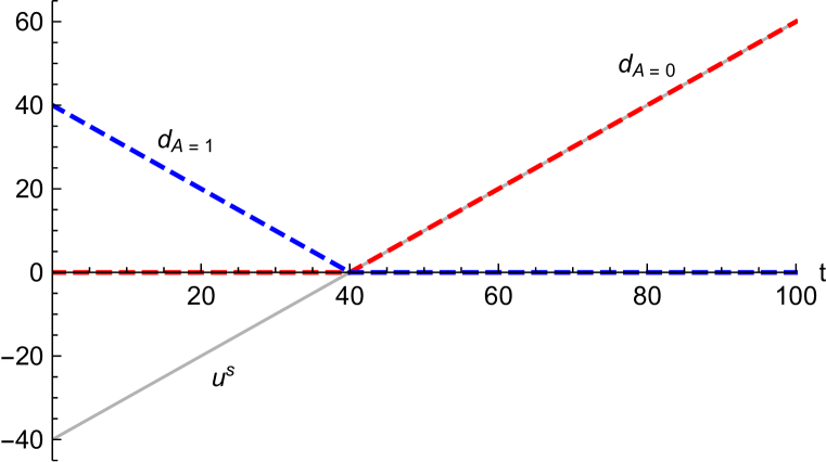
Figure 1: Disagreement cost from accepting ($A=1$) and rejecting ($A=0$) an student.

First consider test mandatory: the student’s test score is observed. If the college chooses to accept regardless of the test score, it bears a disagreement cost of $40-t$ whenever the score is below $40$ (and $0$ otherwise), and so the expected disagreement cost is $\int_{0}^{40}\frac{1}{100}(40-t)\mathrm{d}t=8$. Analogously, if the college instead chooses to reject regardless of test score, it bears an expected disagreement cost of $\int_{40}^{100}\frac{1}{100}(t-40)\mathrm{d}t=18$.

Now consider test blind: the student’s test score is not observed. Here, having no information beyond the uniform prior over the test score, society evaluates the student as if their test score were equal to the expected value $\mathbb{E}[t]=50$. If the college chooses to accept the student, it now faces a disagreement cost of 0: absent test score information, society agrees that the student should be accepted. So if the college were going to accept the student regardless of their test score, then hiding the test score reduces its expected disagreement cost from 8 to 0.

If the test-blind college rejects the student, it does face a disagreement cost: society’s expected utility from admitting the student is $\mathbb{E}[t]-40=10$, and so the college’s disagreement cost from rejection is 10. Nonetheless, hiding the test score reduces the expected disagreement cost of rejecting all applicants from $18$ to $10$.

The upshot is that for either decision the college makes—so long as it is independent of the test score when that is observed—the college can reduce expected disagreement cost by hiding the test score, i.e., going test blind. The fundamental reason is that both disagreement cost curves $d_{A=1}(t)=\max\{40-t,0\}$ and $d_{A=0}(t)=\max\{t-40,0\}$ are convex, as seen in Figure 1. Mathematically, the reduction of expected disagreement cost by going test blind is a consequence of Jensen’s inequality.

Test-optional admissions.

If the college seeks to admit only some students—rather than accepting or rejecting all of them—it might improve upon test blind by going test optional: the student can choose whether to submit their score. For example, consider a college that wants to admit students with test scores above 60, while society’s preferred threshold remains at 40. A test-optional college could commit to treat non-submitters “as if” they have a score of 60, and only accept students with scores (strictly) above 60. If students with scores below 60 (optimally) do not submit their score, this policy implements the college’s desired threshold while resulting in zero disagreement cost. (Society’s expected utility from admitting a non-submitting student is $\mathbb{E}[t|\text{non-submission}]-40=-10$, so society agrees that all the non-submitters should be rejected.)

A tradeoff.

In general, a college faces a tradeoff between using information to make better decisions and not seeing information to reduce disagreement costs. We explore this tradeoff in the rest of the paper. We study how test-optional colleges decide which applicants to admit, how students choose whether to submit test scores, and how the resulting outcomes differ from a test-mandatory benchmark.

4 A Model of Admissions under Social Pressure

We model a student applying to a college, with a broader “society” playing a passive role. The student can be viewed as a representative applicant; we will sometimes use the plural students for exposition. Society represents any external group that might scrutinize admission decisions and has preferences over who ought to be admitted: alumni, parents, local governments, the popular press, and even the judicial branch.

The student is endowed with some publicly observable characteristics and a test score, which is their private information. In a test-mandatory regime, the student mechanically submits their test score, making it public to the college and society. In a test-optional regime, the student chooses whether to submit their score. In either regime, the college chooses whether to admit the student based on their observable characteristics and, if submitted, their test score. Both the college and society have preferences over whether the student should be admitted as a function of their observables and their true test score. The college also places some weight on reducing disagreement between its admission decision and the decision society would want it to make, given all available information.

4.1 Model Primitives

Observables and test scores.

Formally, the student/applicant has a type $(x,t)\in\mathcal{X}\times\mathbb{R}$, where $x$ is an observable (or vector of observables) and $t$ is the test score. The distribution of observables is given by $F_{x}$ and the test score has conditional distribution $F_{t|x}$.

The observable $x$ is public information to all players. The test score $t$ is private information to the student, which may be submitted ($S=1$) or not ($S=0$). Submitting the score makes it observable to all other players. Our primary interest is in two college admission regimes: test mandatory, in which test scores must be submitted, and test optional, in which scores may be submitted. We will also talk about test blind, wherein the score cannot be submitted.

Preferences.

The college decides whether to admit the student (denoted $A=1$) or not ($A=0$), based on observables $x$ and, if submitted, the test score $t$. The student strictly prefers a higher probability of being admitted. Society’s utility and the college’s material or “underlying” utility if the student is accepted are given, respectively, by

$$u^{s}(x,t) :=v^{s}(x)+w^{s}(x)t,$$

$$u^{c}(x,t) :=v^{c}(x)+w^{c}(x)t,$$

where the superscripts have the obvious mnemomic (society and college), and each $w^{i}(\cdot)>0$ for $i=s,c$. We view monotonicity of these preferences in the test score as natural; the affine specifications aid subsequent interpretation and tractability. Both society’s and the college’s underlying utility are normalized to $0$ if the student is not admitted.

In addition to its underlying utility, the college suffers disutility from social pressure on its admission decision. To formalize that disutility, let $t^{s}$ denote the test score society treats the student as having; this will be determined endogenously. Anticipating equilibrium, think of $t^{s}=t$ if the score is submitted, and $t^{s}=\mathbb{E}[t|x,S=0]$ under non-submission. For any $t^{s}$, society’s disagreement with the college’s decision is given by

$$d(x,t^{s},A):=\begin{cases}\max\{u^{s}(x,t^{s}),0\}&\text{if }A=0,\\ \max\{-u^{s}(x,t^{s}),0\}&\text{if }A=1.\end{cases}$$ (1)

The assumed linearity of $u^{s}(x,t)$ in the test score $t$ means that we can interpret $u^{s}(x,t^{s})$ as society’s expected benefit from admitting the student when $t^{s}$ is the expected test score given all available information. Hence, society’s disagreement can be understood as society’s benefit if it were to decide on admissions instead of the college: there is no disagreement if, given the available information, society’s preferred decision is the same as the college’s decision; but when there is a conflict in preferred decisions, then disagreement is linear in the magnitude of society’s expected benefit from its preferred decision. As before, the monotonicity here is natural; linearity is for tractability.

The college’s overall payoff $U^{c}$ is its underlying utility less the (scaled) disagreement:

$$U^{c}(x,t,t^{s},A):=Au^{c}(x,t)-\delta d(x,t^{s},A),$$ (2)

where $\delta>0$ is a parameter capturing the extent of social pressure on the college. We refer to $\delta d(\cdot)$ as the disagreement cost to the college.

Admissions policies.

The college’s admissions policy has two components, one of which—how to treat students who don’t submit test scores—is irrelevant under test mandatory.

First, given the student’s observable $x$, we assume that the college treats non-submission of a test score as equivalent to some specific test score, which we call the imputation. More precisely, there is an imputation rule $\tau:\mathcal{X}\to[-\infty,+\infty]$, with $\tau(x)$ the imputation for observable $x$. We will be interested in two settings: either the college can choose the imputation rule arbitrarily, which we call flexible imputation, or the imputation rule is exogenously given, which we call restricted imputation.

Second, the college chooses an acceptance rule $\alpha:\mathcal{X}\times[-\infty,+\infty]\to[0,1]$, where $\alpha(x,\hat{t})$ is the probability of admitting a student with observable $x$ and imputed/submitted test score $\hat{t}$. We stress that the acceptance rule cannot (directly) condition on the student’s true test score, and it does not distinguish between imputed and submitted scores—this captures our notion that imputing a score means treating a non-submitting student as if they have submitted that imputed score. As in Chan and Eyster (2003), we assume that $\alpha$ must be monotonic in the sense that for any $x$, $\alpha(x,\cdot)$ is weakly increasing.

College’s problem.

Since the college’s acceptance rule is monotonic, there is a simple best response for the student: submit their score if $t>\tau(x)$ and don’t submit if $t\leq\tau(x)$. We restrict attention to the student playing this strategy. Given this student strategy, we assume society is Bayesian in evaluating the student. In particular, if the student submits their test score, then $t^{s}=t$; if the student does not submit, then $t^{s}=L(\tau(x)|x)$, where $L$ (mnemonic for “lower expectation”) is defined by

$$L(t^{\prime}|x):=\mathbb{E}[t|t\leq t^{\prime},x].$$

The college’s problem is to choose—commit to—its imputation rule $\tau$ (under test optional with flexible imputation) and its acceptance rule $\alpha$, to maximize its expected payoff $U^{c}$, anticipating the student’s best response and society’s Bayesian inferences.

4.2 Ex-Post Utility

Observe that when $t^{s}=t$, as will be the case if the student submits their score, Equation 1 and Equation 2 imply that the college’s net benefit from admitting the student is given by

$$U^{c}(x,t,t,1)-U^{c}(x,t,t,0) =u^{c}(x,t)-\delta\left[d(x,t,1)-d(x,t,0)\right]$$

$$=u^{c}(x,t)+\delta u^{s}(x,t)$$

$$\propto\frac{1}{1+\delta}u^{c}(x,t)+\frac{\delta}{1+\delta}u^{s}(x,t)$$

$$=:u^{*}(x,t).$$ (3)

We refer to $u^{*}(x,t)$ as the college’s ex-post utility. For a score-submitting student, our disagreement cost formulation implies that the college’s net benefit from admission is equivalent (i.e., proportional to) to a convex combination of the college’s underlying utility and society’s utility. If the student submits their score, the college’s payoff is maximized by admitting the student if and only if (modulo indifference) $u^{*}(x,t)>0$.

For $i\in\{c,s\}$, we refer to $\underline{t}^{i}(x)$ such that $u^{i}(x,\underline{t}^{i}(x))=0$ as the college/society’s test-score bar for admission: it is the score threshold such that each would—if unencumbered by social pressure—prefer to admit the student with observable $x$ if and only their score is above that threshold. We denote the ex-post utility bar by $\underline{t}^{*}(x)$; it is defined by $u^{*}(x,\underline{t}(x))=0$ and is the threshold above which, accounting for social pressure, the college wants to admit the student. We say that the college is less selective than society at observable $x$ if $\underline{t}^{c}(x)<\underline{t}^{s}(x)$, while it is more selective if $\underline{t}^{c}(x)>\underline{t}^{s}(x)$. In either case, the ex-post utility bar $\underline{t}^{*}(x)$ is in between the two parties’ bars, and it monotonically shifts from $\underline{t}^{c}(x)$ to $\underline{t}^{s}(x)$ as the social-pressure intensity parameter $\delta$ increases.

2(b) illustrates with a leading specification in which $x\in\mathbb{R}$, and for each $i\in\{c,s\}$, $u^{i}(x,t)=a^{i}+x+w^{i}\times t$. In this specification, the college weights test scores more than society when $w^{c}>w^{s}$, and weights test scores less than society when $w^{c}<w^{s}$. The three lines indicate the respective test-score bars at each $x$. When the college weights test scores less, as in the figure’s left panel, at low $x$ it is more selective (has a higher bar) than society, but at high $x$ it is less selective (has a lower bar); and the reverse when the college weights test scores more than society, as in the right panel.

Figure 2: Test score admission bars for society ($\underline{t}^{s}$), the college’s underlying utility ($\underline{t}^{c}$), and ex-post utility ($\underline{t}^{*}$). For this figure, $x\in\mathbb{R}$ and $u^{i}=a^{i}+x+w^{i}\times t$.

(a) College weights tests less than society: $w^{c}<w^{s}$.

(b) College weights tests more than society: $w^{c}>w^{s}$.

4.3 Discussion of the Model

4.3.1 Imputation and acceptance rules

A test-optional admissions policy in our model is an imputation rule paired with a monotonic acceptance rule. We view the framework of imputation as an appealing and versatile way to capture how colleges may actually treat missing test scores. For example, it allows us to discuss cultural or legal norms about how non-submitters should be treated (as elaborated below). Monotonicity of the acceptance rule is without loss if students can “freely dispose” of test scores—a student with test score $t$ can costlessly reduce it to any value less than $t$.

At a theoretical level, however, the natural alternative would be to specify an admissions policy as an arbitrary mapping from observables, whether the student submits their score, and the score if submitted, to an admissions probability. We show in Appendix C that the outcome under this alternative is the same as that under flexible imputation. In this sense, neither imputations nor monotonic acceptance rules are restrictive.

4.3.2 Restricted imputation rules

With flexible imputation, the college can arbitrarily choose how to impute missing test scores. With restricted imputation, we consider the other extreme, in which an imputation rule is exogenously specified. Although our analysis will not have any results tied to particular restricted imputation rules, we allow for them to cover some colleges’ practice of publicly promising not to “penalize” or “disadvantage” students who don’t submit scores. We interpret such promises as mapping to some version of what we call the no adverse inference imputation rule, $\tau(x)=\mathbb{E}[t|x]$. Contrast this expression to the Bayesian imputation rule used by society, in which $t^{s}=\mathbb{E}[t|x,S=0]$: no adverse inference updates based on observables but not on the choice not to submit. That is, the college imputes test scores as if students who did not submit chose to do so non-strategically.

Even when ignoring the submission decision, the college might condition its expectation not on the full vector of observables but on some subset of relevant components. For instance, if the observable vector $x=(x_{0},x_{1})$ has component $x_{1}$ corresponding to “grades” and component $x_{0}$ corresponding to “demographics” (race, gender, family income, neighborhood of residence), the college might impute $\tau(x)=\mathbb{E}[t|x_{1}]$. This gives the expectation of $t$ conditional on grades but not on demographics (and not on the decision to submit). Indeed, certain features such as race or gender may be legally protected categories, in which case it might be forbidden to impute scores differently based on these factors—even if they are in fact predictive of test scores. In the limiting case, a college might deem all observables irrelevant, in which case it would impute $\tau(x)=\mathbb{E}[t]$ identically for all applicants.

4.3.3 Key assumptions

Simplifications.

Our model makes a number of simplifying assumptions in order to focus on the channel of social pressure as an explanation for going test optional. For instance, we abstract away from a student’s decision of how much to study for, or whether to even take, the test. Instead, we endow students with a test score. We then give the college and society a reduced form preference over these test scores rather than microfounding any inference over underlying ability. We also don’t model the student’s application decision.

One other simplifying assumption to flag is that we model the college as having a fixed underlying utility threshold for admission. In particular, even if a switch from test mandatory to test optional leads to a different number of admitted students, the college does not raise or lower its threshold for admission in order to keep its class size constant. We return to this point in the Conclusion.

Student submission behavior.

We assume that students submit a test score if their true score $t$ is strictly above the college’s imputed value $\tau(x)$, and they withhold the score if $t$ is weakly below $\tau(x)$. Higher test scores can only help admission chances.So, as discussed, this strategy guarantees a student the highest chance of admission. While there may be other optimal student strategies (when submitting a test score $t$ would lead to the same acceptance probability as not submitting), a student can safely follow the strategy we focus on even if they do not know which (monotonic) acceptance rule the college is using.

Of course, while the strategy is robust to a student’s uncertainty over the college’s acceptance rule, it is sensitive to the student’s belief about their imputed test score. McManus et al. (2023) show that student submission behavior does appear to vary with the belief about how colleges might impute missing test scores. Admittedly, our model makes the strong “equilibrium assumption” of a correct belief about the imputation.

5 Test-Mandatory Admissions

In a test-mandatory regime, both the college and society always know the student’s score. In light of social pressure, the college simply maximizes its ex-post utility for each $(x,t)$; its admission decision is determined by the ex-post bar.

Proposition 1.

In a test-mandatory regime, the college admits a student with observable $x$ if $u^{*}(x,t)>0$ (equivalently, $t>\underline{t}^{*}(x)$) and rejects the student if $u^{*}(x,t)<0$ (equivalently, $t<\underline{t}^{*}(x)$).

As the social-pressure intensity parameter $\delta$ increases, the college becomes less selective at observable $x$ if, based on its underlying utility, it is more selective than society ($\underline{t}^{c}(x)>\underline{t}^{s}(x)$), and conversely if it is less selective than society. Plainly, the student with observable $x$ benefits in the former case and is harmed in the latter case.

6 Test-Optional Admissions

6.1 Optimal Acceptance Rule

In a test-optional regime, our college has two instruments: the imputation rule and the acceptance rule. Only the imputation rule affects students’ score submission, and in turn the college’s and society’s information. Moreover, the only decision that students make is whether to submit their score. So, no matter the imputation rule, the college’s optimal acceptance rule simply maximizes its ex-post utility given students’ submission behavior. Formally, recalling that $L(\tau(x)|x)$ is the average test score of non-submitters with observable $x$ given the imputation $\tau(x)$:

Lemma 1.

Consider a test-optional regime with any imputation rule $\tau$. The college has an optimal acceptance rule in which a student with observable $x$ and imputed/submitted score $\hat{t}$ is accepted if (i) $\hat{t}>\tau(x)$ and $u^{*}(x,\hat{t})>0$ or if (ii) $\hat{t}=\tau(x)$ and $u^{*}(x,L(\tau(x)|x))>0$, and is rejected otherwise.

Any optimal admission rule must have the college making ex-post optimal decisions on path. The lemma’s acceptance rule also specifies rejecting any student who has a test score below the imputed level but who chooses, off path, to submit. When the non-submitters are accepted, we could replace this behavior with any other monotonic rule and the outcome would be the same. When the non-submitters are rejected, though, monotonicity of the admission rule requires the college to also reject any score submission below the imputed score. In this latter case, commitment to the policy may be necessary: off path, the college may be rejecting students that it ex-post prefers to accept. For example, suppose test scores at some observable $x$ are distributed uniformly between 0 and 100, and the imputation is $\tau(x)=50$. Students with scores between 0 and 50 don’t submit, leading to an average score of 25 for non-submitters. If the college’s ex-post bar for acceptance is in between 25 and 50, say $\underline{t}^{*}(x)=40$, then the college will reject the non-submitters. The college must then reject all off-path submissions of scores below 50, including—ex-post suboptimally—those above its ex-post bar of 40.

6.2 Flexible Imputation

We now turn to studying optimal admission policies under flexible imputation. Clearly, the college can ensure that it is no worse off than under test mandatory: after all, the imputation rule $\tau(\cdot)=-\infty$ ensures that all students submit their scores. But when and how can the college do better?

In choosing its imputation $\tau(x)$ for some observable $x$, the college trades off making better admission decisions with reducing disagreement cost. Raising $\tau(x)$ leads fewer students to submit their test scores. The cost is that the college now has less information with which to make admissions decisions. The benefit is that by pooling together a larger set of test scores (those of the non-submitters), the college can reduce the disagreement cost it bears with society, as we saw in Section 3. In particular, consider two students who are both rejected or both accepted. If their test scores are either both below society’s bar $\underline{t}^{s}(x)$ or both above, the disagreement cost is the same regardless of whether these students submit their scores or are pooled together. But if these students are on opposite sides of society’s bar, then the disagreement cost is lower when the students are pooled together.

When solving for the optimal admissions policy, the college’s problem is separable across observables. That is, we can optimize at each observable $x$ and then “stitch” together the solutions across $x$’s to get the globally optimal admission policy.

Given some fixed $x$, it is useful to consider separately the case in which the college is less selective than society ($\underline{t}^{c}(x)<\underline{t}^{*}(x)<\underline{t}^{s}(x)$) and the case in which it is more selective ($\underline{t}^{s}(x)<\underline{t}^{*}(x)<\underline{t}^{c}(x)$). For both cases, we will assume without loss that the imputation level $\tau(x)$ is set as $\tau(x)\geq\underline{t}^{*}(x)$, and that any submitted score $t>\tau(x)$ is accepted.

College is less selective than society.

When the college is less selective, setting $\tau(x)=\underline{t}^{*}(x)$ and rejecting non-submitters replicates not only the test-mandatory admission decisions, but also the college’s test-mandatory payoff. This is because all of the scores being pooled together are below society’s acceptance threshold $\underline{t}^{s}(x)$. Furthermore, the college does worse if it sets $\tau(x)>\underline{t}^{*}(x)$ and then rejects non-submitters: it is now rejecting students that it preferred to accept even if it had to pay a disagreement cost to do so. Altogether, if the college rejects non-submitters, then it cannot improve on setting $\tau(x)=\underline{t}^{*}(x)$ and replicating the test-mandatory outcome.

The college might improve on test mandatory, however, by accepting non-submitters at some observable. Monotonicity of the acceptance rule means that the college would then accept all students with this observable. With all of these students being accepted, the college would minimize disagreement costs by setting the imputation level to infinity, so that none of these students submit scores. Of course, relative to test mandatory, the college would then be admitting too many low-scoring students. Hence:

Proposition 2.

Consider flexible imputation and some observable $x$. When the college is less selective than society ($\underline{t}^{c}(x)<\underline{t}^{*}(x)<\underline{t}^{s}(x)$), it is optimal for the college to either:

1. Impute $\tau(x)=\infty$ and accept students regardless of imputed/submitted score $\hat{t}$; or

2. Replicate the test-mandatory outcome by imputing $\tau(x)=\underline{t}^{*}(x)$, rejecting students with imputed/submitted score $\hat{t}\leq\underline{t}^{*}(x)$, and accepting students with $\hat{t}>\underline{t}^{*}(x)$.

3(a) and 3(b) illustrate the two possibilities.

Figure 3: College’s test-optional payoff as a function of the imputed test score, when the college is less selective than society.

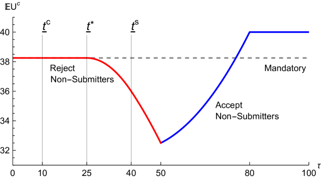
(a) The college’s payoff is maximized by setting $\tau=\infty$ and accepting non-submitters.

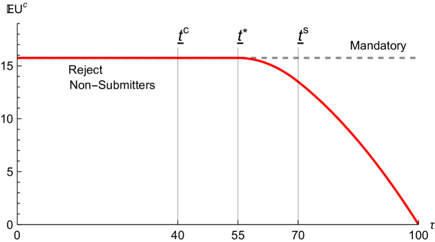
(b) The college’s payoff is maximized by setting $\tau=\underline{t}^{*}$ and rejecting non-submitters.

Fix some observable $x$. The distribution of test scores given $x$ is $t\sim U[0,100]$. Utilities are $u^{c}(x,t)=t-\underline{t}^{c}$, $u^{s}(x,t)=t-\underline{t}^{s}$, and $\delta=1$, implying $\underline{t}^{*}=\frac{1}{2}(\underline{t}^{c}+\underline{t}^{s})$.

College is more selective than society.

Let us turn to observables at which the college is more selective than society. Unlike when the college is less selective, the college can improve on test mandatory by imputing the ex-post optimal bar, rejecting non-submitters, and accepting submitters. Pooling together the scores of all the rejected students now reduces disagreement cost because society prefers to reject some of those students (those with $t<\underline{t}^{s}(x)$) and accept others ($t\in(\underline{t}^{s}(x),\underline{t}^{*}(x)$). In general, the college might do even better by choosing a higher imputation, altering the set of admitted students.

Proposition 3.

Consider flexible imputation and some observable $x$. When the college is more selective than society ($\underline{t}^{s}(x)<\underline{t}^{*}(x)<\underline{t}^{c}(x)$), the college optimally chooses imputation $\tau(x)\in[\underline{t}^{*}(x),\underline{t}^{c}(x)]$; it rejects students with imputed/submitted score $\hat{t}\leq\tau(x)$ and it accepts students with $\hat{t}>\tau(x)$.

The proposition’s proof establishes that the optimal $\tau(x)$ is determined by comparing the function $L(\cdot|x)$, which gives the average test score of non-submitters, with society’s bar $\underline{t}^{s}(x)$. Specifically, letting $t^{\circ}$ be a score at which $L(t^{\circ}|x)=\underline{t}^{s}(x)$, the college sets

$$\tau(x)=\begin{cases}\underline{t}^{*}(x)&\text{ if }t^{\circ}\leq\underline{t}^{*}(x)\\ t^{\circ}&\text{ if }t^{\circ}\in(\underline{t}^{*}(x),\underline{t}^{c}(x))\\ \underline{t}^{c}(x)&\text{ if }t^{\circ}\geq\underline{t}^{c}(x)\end{cases}.$$

For the intuition behind Proposition 3, consider the case in which $t^{\circ}\in(\underline{t}^{*}(x),\underline{t}^{c}(x))$. The optimal admissions policy then involves setting $\tau(x)=t^{\circ}$, rejecting non-submitters, and accepting submitters. This imputation makes society indifferent over whether to accept the pool of non-submitters, as their expected test score is $L(\tau(x)|x)=\underline{t}^{s}(x)$. Moreover, society wants to accept any submitter, since their score is $t\geq\tau(x)>\underline{t}^{s}(x)$. So the disagreement cost is zero. Now consider a marginal change of the imputation level $\tau(x)$ from $t^{\circ}$ to $t^{\prime}$. On the one hand, raising the imputation level $\tau(x)$ to $t^{\prime}>t^{\circ}$ cannot help. Doing so and then rejecting the larger pool yields the same set of admitted students and the same disagreement cost as setting $\tau(x)=t^{\circ}$ and then rejecting students with scores $t\in(t^{\circ},t^{\prime}]$; there is no benefit from pooling the scores of these marginal students with those below $t^{\circ}$ since society does not strictly prefer to reject the pool of non-submitters. But the latter policy is dominated by the originally proposed policy of setting $\tau(x)=t^{\circ}$ and accepting students with scores $t\in(t^{\circ},t^{\prime}]$, as they provide positive ex-post utility. On the other hand, lowering the imputation level to $t^{\prime}<t^{\circ}$ also cannot help. Doing so and then rejecting students with $t\in(t^{\prime},t^{\circ}]$ yields the same set of admitted students but higher disagreement cost, since society strictly prefers to reject the pool of non-submitters when $\tau(x)=t^{\prime}$; doing so and then accepting students with $t\in(t^{\prime},t^{\circ}]$ yields a worse set of admitted students from the college’s perspective, as $t<\underline{t}^{c}(x)$, but identical (zero) disagreement cost.

Figure 4 illustrates two examples of Proposition 3. Panel 4(a) shows a case in which the optimal $\tau(x)$ is in $(\underline{t}^{*}(x),\underline{t}^{c}(x))$. Panel 4(b) shows a case in which the optimal $\tau(x)$ is equal to $\underline{t}^{c}(x)$, and the college achieves its first best: it accepts students if and only if $t>\underline{t}^{c}(x)$, and it incurs no disagreement cost. Although not illustrated in the figure, it is also possible that the optimal $\tau(x)=\underline{t}^{*}(x)$.

Figure 4: College’s test-optional payoff as a function of the imputed test score, when the college is more selective than society.

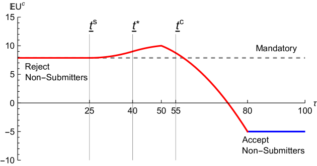
(a) The college’s payoff is maximized by setting $\tau\in(\underline{t}^{*},\underline{t}^{c})$ and rejecting non-submitters.

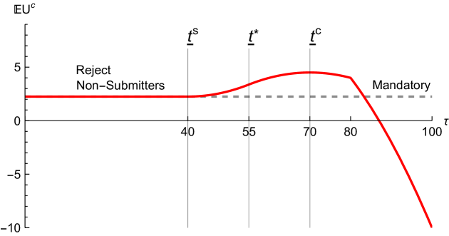
(b) The college achieves its first best by setting $\tau=\underline{t}^{c}$ and rejecting non-submitters.

Fix some observable $x$. The distribution of test scores given $x$ is $t\sim U[0,100]$. Utilities are $u^{c}(x,t)=t-\underline{t}^{c}$, $u^{s}(x,t)=t-\underline{t}^{s}$, and $\delta=1$, implying $\underline{t}^{*}=\frac{1}{2}(\underline{t}^{c}+\underline{t}^{s})$.

How are students affected?

The outcomes of a college-optimal admissions policy under test-optional admissions have clear-cut and intuitive implications for student welfare relative to the outcomes of test-mandatory admissions.

Students benefit from test optional at observables where the college is less selective than society. Specifically, at these observables, Proposition 2 implies that either the college replicates the test-mandatory admissions, or it admits all students. In the latter case, high-scoring students (with $t>\underline{t}^{*}(x)$)) are indifferent between test optional and test mandatory, but low-scoring students ($t<\underline{t}^{*}(x)$) strictly benefit.

By contrast, students are harmed by test optional at observables where the college is more selective than society. Specifically, Proposition 3 implies that when the optimal imputation is $\tau(x)=\underline{t}^{*}(x)$, the test-mandatory outcome is replicated for all students. But when the optimal imputation is $\tau(x)>\underline{t}^{*}(x)$, intermediate-scoring students (with $t\in(\underline{t}^{*}(x),\tau(x)]$) are rejected under test optional while they would have been accepted under test mandatory, whereas the outcomes for low- and high-scoring students ($t<\underline{t}^{*}(x)$ and $t>\tau(x)$, respectively) are unchanged.

6.3 Restricted Imputation

We now turn to test-optional admissions when the imputation rule $\tau(\cdot)$ is exogenously given. The college only optimizes its acceptance rule. As discussed in Subsection 4.3.2, many colleges announce a policy that we interpret as no adverse inference imputation. Restricted imputation also subsumes test-blind admissions, as that is equivalent to $\tau(\cdot)=\infty$.

The optimal acceptance rule.

As with flexible imputation, we can solve for an optimal acceptance rule under restricted imputation separately for each observable $x$. An optimal acceptance rule readily follows from Lemma 1:

Proposition 4.

Consider some observable $x$ and imputation level $\tau(x)$. An optimal acceptance rule for the college is as follows. A student with submitted score $t>\tau(x)$ is accepted if and only if $t>\underline{t}^{*}(x)$; a student with submitted score $t<\tau(x)$ is rejected; and a student with imputed/submitted score $\tau(x)$ is accepted if and only if $L(\tau(x)|x)>\underline{t}^{*}(x)$.

The proposition says that the college’s acceptance rule on path is determined by comparing a student’s expected score—the score if submitted, or $L(\tau(x)|x)$ if not submitted—with the ex-post bar. (Submission of $t\leq\tau(x)$ only occurs off path.) Whether the college is more or less selective than society does not affect the college’s optimal acceptance rule; the distinction matters under flexible imputation (Subsection 6.2) only because it affects the optimal imputation.

To better understand the admissions policy under restricted imputation, we can consider exogenously varying the imputation $\tau(x)$ at a given $x$. In that case, there is a threshold $T(x)$ such that if $\tau(x)<T(x)$, then it is optimal to reject non-submitters, whereas if $\tau(x)>T(x)$, then it is optimal to accept non-submitters. Figure 3 and Figure 4 illustrate, at some fixed observable $x$, how the college’s payoff and its decision of whether to accept non-submitters may depend on the imputation level.

How are students affected?

Whether students at an observable $x$ benefit from test optional under restricted imputation (relative to test mandatory) depends on how the imputation level $\tau(x)$ and the lower expectation $L(\tau(x)|x)$ compare with the ex-post bar $\underline{t}^{*}(x)$. To understand how these vary with observables, we must make further assumptions.

Accordingly, define a path of increasing observables as a parameter $q\in[0,1]$ determining the observable $x(q)$, with the following properties: (i) $u^{c}(x,t)=v^{c}(x)+t$ and $u^{s}(x,t)=v^{s}(x)+t$, with $v^{c}(x(q))$ and $v^{s}(x(q))$ both increasing in $q$; (ii) the distribution of $t|x(q)$ is MLRP-increasing in $q$, and (iii) $\tau(x(q))$ is increasing in $q$. Property (i) guarantees that the ex-post bar $\underline{t}^{*}(x(q))$ is decreasing in $q$, while properties (ii) and (iii) guarantee that the expected test score conditional on not submitting, $L(\tau(x(q))|x(q))$, is increasing in $q$. Note that property (iii) is implied by property (ii) when $\tau$ is the no adverse inference rule defined by $\tau(x)=\mathbb{E}[t|x]$.

A path of increasing observables yields straightforward implications for which students benefit or are harmed by test-optional admissions with restricted imputation, as can be seen using Figure 5. Students with “low” observables (those with $q$ such that $\tau(x(q))<\underline{t}^{*}(x(q))$) are unaffected. Under both test-optional and test-mandatory admissions, these students are accepted if and only if their test score is above the ex-post bar. Students with “medium” observables ($q$ such that $\tau(x(q))>\underline{t}^{*}(x(q))$ but $L(\tau(x(q))|x(q))<\underline{t}^{*}(x)$) are harmed. If their test score is low ($t\leq\underline{t}^{*}(x)$) then they are rejected under both regimes, and if their test score is high ($t>\tau(x)$) then they are admitted either way. But if their score is in between, they are accepted under test mandatory and rejected under test optional. Finally, students with “high” observables ($q$ such that $L(\tau(x(q))|x(q))>\underline{t}^{*}(x)$) benefit. If their test score is high ($t>\underline{t}^{*}(x(q))$) then they are admitted under both regimes. If their score is low ($t\leq\underline{t}^{*}(x(q))$), they are rejected under test mandatory and are accepted without submitting their score under test optional.

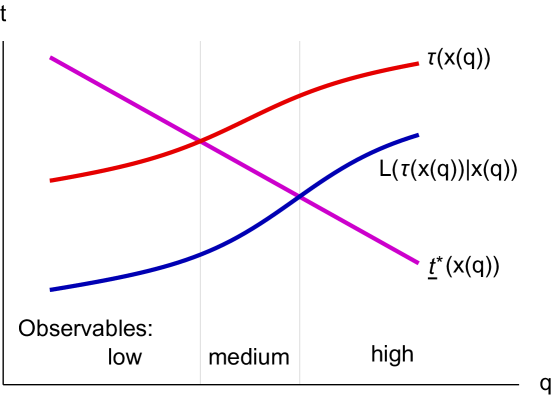
Figure 5: Restricted imputation along a path of increasing observables.

Restricted vs. flexible imputation.

Under restricted imputation, given a path of increasing observables, students with good observables benefit under test optional while students with medium observables are harmed. By contrast, under flexible imputation, it is students with observables at which the college is less selective than society that benefit and those with observables at which the college is more selective that are harmed. Looking back at Figure 2, we see that these predictions may go in the same qualitative direction, or may go in opposite directions. In the figure’s left panel, where the college weights tests less than society, the college is less selective than society at higher observables. Hence, students with higher observables benefit from test optional under both flexible and restricted imputation. In Figure 2’s right panel, where the college weights tests more than society, we have the reverse: the college is more selective at higher observables. In this case, the predictions about which students benefit from test optional flip depending on whether imputation is flexible or restricted.

Under flexible imputation, the college always benefits (at least weakly) from going test optional. Notably, this benefit accrues at every observable $x$. By contrast, under restricted imputation, the college may or may not benefit from going test optional at any specific $x$—it depends on the imputation level $\tau(x)$. Consequently, aggregating across observables, the college may or may not benefit from going test optional.

We now turn to an extended example with specific assumptions that allow us to say more about when a college benefits from not seeing test scores absent flexible imputation. The example is in the context of a college’s response to a ban on affirmative action.

7 Effects of a Ban on Affirmative Action

This section illustrates how, within our framework, banning affirmative action can push a college from test-mandatory admissions to test-blind admissions.

In a nutshell, our idea is as follows. There are two groups of students. Relative to society, the college has a preference for admitting students from the group that has lower test scores on average. When affirmative action is allowed, the college can treat applicants from different groups differently. In that case, the college always prefers test mandatory, since observing test scores lets it determine which applicants to accept from each group. But if affirmative action is banned, the college must use a single admissions rule for both groups. Now the college wants to put less weight on tests than does society, since a low test score is associated with being from the college’s favored group. This disagreement can push the college to want to switch to test blind.

Some commentators have also suggested that banning affirmative action may induce colleges to avoid test score mandates (e.g., New Yorker, January 2022). One rationale is that going test blind can suppress evidence of score differentials across groups, which could have been used in lawsuits alleging that a college makes illegal decisions based on group identity. Our story is somewhat distinct, but complementary. We assume that with a ban on affirmative action, the college cannot directly condition on group identity. But in response, the college wants to put less weight on tests. Hiding test scores allows the college to do so in a way that generates less disagreement with society. This can interpreted as protecting the college from criticism of how much weight it places on different elements of an application.

7.1 A Model of Affirmative Action

There are two potentially observable non-test dimensions, $x=(x_{0},x_{1})$. Dimension $x_{0}$ is binary, with realizations in $\{r,g\}$ (red and green). Dimension $x_{1}$, which may represent some aggregate of GPA and/or extra-curricular achievement, takes continuous values in $\mathbb{R}$. For simplicity, test scores are binary, with values normalized to $0$ and $1$.

The college and society have identical preferences over all factors except for the type dimension $x_{0}$. Society does not care about this dimension, but all else equal, the college wants to admit green types over red types. Specifically, extending our leading linear specification discussed at the end of Subsection 4.2, we assume that

$$u^{s}(x,t) =x_{1}+t,$$

$$u^{c}(x,t) =x_{1}+t+\beta{1}{1}_{x_{0}=g}-c,$$

with $\beta>c>0$, and ${1}{1}_{x_{0}=g}$ an indicator for green types. The parameter $\beta$ is the bonus the college gives to green types over red types. The parameter $c$ is not essential to our analysis, but it allows for the college and society to have different test-score bars for both red and green students. It can be interpreted as the (opportunity) cost for a college of admitting any student. We have normalized the analogous constant in society’s utility to zero. The assumption $\beta>c>0$ implies that the college has a lower test-score bar than society for green types and a higher one for red types. Note that the the college’s ex-post utility is

$$u^{*}(x,t)=x_{1}+t+\frac{\beta}{1+\delta}{1}{1}_{x_{0}=g}-\frac{c}{1+\delta}.$$

Let $x_{0}=g$ with probability $q\in(0,1)$ and $x_{0}=r$ with probability $1-q$. We assume that the distribution of test scores depends on $x$ only through $x_{0}$: $\Pr(t=1|x=(x_{0},x_{1}))=p_{x_{0}}\in(0,1)$. Our primary interest is in the case of $p_{r}>p_{g}$, meaning that green types, which are favored by the college, have a worse distribution of test scores. This may correspond to green students being an underrepresented demographic group, for instance. But we also allow for the opposite case of $p_{r}<p_{g}$, in which the college’s favored group has a better test score distribution. Here, green students may correspond to those from rich families, who have better access to test preparation, and are favored by the college because of donor considerations. If the green students correspond to legacy applicants, it may be that either $p_{r}<p_{g}$ or $p_{r}>p_{g}$.

We take $x_{1}$ to be independent of both $x_{0}$ and $t$. For tractability, we also assume that $x_{1}$ is uniformly distributed over a large enough interval. Specifically, $x_{1}\sim U[\underline{x}_{1},\overline{x}_{1}]$, with $\underline{x}_{1}<c-\beta-1$ and $\overline{x}_{1}>c$. The inequality on $\underline{x}_{1}$ guarantees that there are students with $x_{1}$ low enough that neither the college nor society wants to admit them, even if they are otherwise as desirable as possible ($x_{0}=g$ and $t=1$). The inequality on $\overline{x}_{1}$ guarantees that there are students with $x_{1}$ high enough that the college and society want to admit them even if they are otherwise as undesirable as possible ($x_{0}=r$ and $t=0$).

We will consider the college’s choice over whether to be test mandatory or test blind in two observability regimes. First, we allow both dimensions of $x$ to be observable, which we call affirmative action allowed. Then we consider only $x_{1}$ to be observable, with the dimension $x_{0}$ unobservable; we call this regime affirmative action banned. We interpret the switch from the first to the second regime as a policy change where society—which does not intrinsically care about $x_{0}$—bans the use of that dimension in admissions. This may represent a law or court decision forbidding the use of race or legacy status in admissions.

7.2 Results

Affirmative action allowed.

Consider first the case when affirmative action is allowed.

Under test mandatory, the college can choose a distinct threshold of $x_{1}$ above which to admit students at each $(x_{0},t)$ pair. This threshold is determined by setting the ex-post utility to $0$. Since the college favors green students, its $x_{1}$ threshold will be lower by $\beta/(1+\delta)$ for green students than for red students at each score level $t$. From society’s perspective, the college uses an $x_{1}$ threshold that is too low for green students and too high for red students—but crucially, the gap between society’s preferred threshold and what the college uses does not vary with $t$.

Under test blind, the college chooses an admissions threshold on dimension $x_{1}$ that depends on the student’s type $x_{0}$ but not the test score $t$. However, $x_{0}$ is informative about $t$: the college and society evaluate students of type $x_{0}$ as if they have the expected test score $\mathbb{E}[t|x_{0}]=p_{x_{0}}$. If $p_{r}>p_{g}$, the college’s preference for green students is countered by the fact that green students have lower test scores on average than red students. So the college will now use a lower $x_{1}$ threshold for green students than red students only if its preference parameter $\beta$ is sufficiently large: specifically, if and only if $\beta/(1+\delta)>p_{r}-p_{b}$. Regardless, the gap between the college’s chosen $x_{1}$ threshold and society’s preferred threshold is the same as under test mandatory, for any test score $t$—that gap did not depend on the test score, and utilities are linear in the test score.

We can establish:

Proposition 5.

If affirmative action is allowed, then the college prefers test mandatory to test blind.

The reason is that going test blind leads to a set of students that the college prefers less, but in the current specification there is never a countervailing benefit of reducing disagreement cost. The latter point stems from two sources. First, as noted above, for any given $x_{0}$ type (and test score, under test mandatory), the gap between society’s preferred $x_{1}$ threshold and what the college uses is independent of the regime, even though these thresholds do shift across regimes. Second, our assumption of a uniform distribution of $x_{1}$ means that the total disagreement cost for students of a given $x_{0}$ type (at a given test score, or averaging over test scores) only depends on the size of the gap.

Affirmative action banned.

Now consider the case when affirmative action is banned.

Under test mandatory, the observed test score is informative about a student’s type $x_{0}$. Specifically, since there are a fraction $q$ of green types in the population and the probability of test score $t=0$ for a student of type $x_{0}$ is $1-p_{x_{0}}$, we compute the probability of a student being green conditional on $t=0$ as

$$P_{g}^{0}:=\Pr(x_{0}=g|t=0)=\frac{q}{q+(1-q)\frac{1-p_{r}}{1-p_{g}}}.$$

Analogously, conditional on $t=1$, the probability of a green type is

$$P_{g}^{1}:=\Pr(x_{0}=g|t=1)=\frac{q}{q+(1-q)\frac{p_{r}}{p_{g}}}.$$

Let $\Delta:=P_{g}^{0}-P_{g}^{1}$ be the difference between these two quantities, i.e., a low test score implies a $\Delta$ higher probability of $x_{0}=g$ than a high test score. Note that $\Delta>0$ if $p_{r}>p_{g}$, whereas $\Delta<0$ if $p_{r}<p_{g}$. Based on the inference of $x_{0}$ from $t$, the college’s underlying utility gives a bonus of $\beta\Delta$ to students with low test scores relative to those with high scores. As a result, the college now values a high test score $1-\beta\Delta$ units higher than a low score, whereas society still values it 1 unit higher. That is, unlike when affirmative action is allowed, the gap between society’s preferred $x_{1}$ admissions threshold and what the college chooses now varies with the test score. We impose the assumption that $\beta\Delta<1$, so the college still prefers students with higher test scores.

There is now an avenue for test blind to help the college. Under test blind, since the college evaluates all students as having $\Pr(x_{0}=g)=q$ and $\mathbb{E}[t]=qp_{g}+(1-q)p_{r}$, it is as if the college’s utility from any student is $x_{1}+\mathbb{E}[t]+q\beta-c$. Analogously, it is as if society’s utility from any student is $x_{1}+\mathbb{E}[t]$. If $c=q\beta$, which means the college and the society seek to admit the same number of students overall, then it is as if their utilities agree, and the college implements its preferred admissions policy—subject to being test blind and no affirmative action—at zero disagreement cost. More generally, the disagreement cost is always lower under test blind than test mandatory. Whether the reduced disagreement cost outweighs the allocative loss from being test blind depends on parameters, specifically the intensity of social pressure $\delta$ and the college’s bonus to low-scoring students $\beta\Delta$.

Proposition 6.

Suppose affirmative action is banned. If $(1+\delta)(2\beta\Delta-1)\geq(\beta\Delta)^{2}$, then the college prefers test blind, and otherwise the college prefers test mandatory.

Recall we assume $\beta\Delta<1$. Proposition 6 implies that if $\beta\Delta\leq 1/2$, the college always prefers test mandatory: the allocative losses (“admission mistakes”) from not observing test scores are larger than those from simply implementing society’s preferred decision rule and incurring no disagreement. When $\beta\Delta\in(1/2,1)$, there is a trade-off, and test blind will be preferred if the intensity of social pressure, $\delta$, is sufficiently large. The following corollary develops this and other comparative statics.

Corollary 1.

Suppose that affirmative action is banned ($x_{0}$ is unobservable) and that a low test score is associated with $x_{0}=g$ ($\Delta>0$).

1. There is some $\beta^{*}\in\left(\frac{1}{2\Delta},\frac{1}{\Delta}\right)$ such that the college prefers test mandatory when $\beta<\beta^{*}$ and prefers test blind when $\beta>\beta^{*}$.

2. There is some $\Delta^{*}\in\left(\frac{1}{2\beta},\frac{1}{\beta}\right)$ such that the college prefers test mandatory when $\Delta<\Delta^{*}$ and prefers test blind when $\Delta>\Delta^{*}$.

3. If $\beta\Delta\leq 1/2$, then the college prefers test mandatory for all $\delta$; if $\beta\Delta\in(1/2,1)$, then there is some $\delta^{*}>0$ such that the college prefers test mandatory when $\delta<\delta^{*}$ and prefers test blind when $\delta>\delta^{*}$.

7.3 Society’s Preferences

We now consider society’s payoff under different affirmative action and testing regimes. Society’s realized utility for an individual student is $Au^{s}(x,t)$, where the dummy variable $A$ indicates whether the student is admitted. We assume that society’s objective is to maximize its expected utility across the pool of applicants.

Proposition 7.

Society’s preferences over affirmative action and testing regimes are as follows:

1. Fixing the testing regime as mandatory or blind, society prefers banning affirmative action to allowing affirmative action.

2. Fixing affirmative action as banned or allowed, society prefers test mandatory to test blind.

3. Suppose society chooses the affirmative action regime and then the college chooses the testing regime. Then banning affirmative action can harm society. In particular, if $\beta\Delta\in\left(1/2,1\right)$, there exist thresholds $0<\underline{\delta}\leq\overline{\delta}<\infty$ such that (i) if affirmative action is banned, the college chooses test blind if $\delta>\underline{\delta}$, and (ii) society is harmed by banning affirmative action if $\delta>\overline{\delta}$, while it benefits if $\delta<\overline{\delta}$.

The first two parts of the proposition are intuitive, since society does not want the admission decision to depend on whether a student is red or green (which suggests part 1) but does want the decision to depend on the test score (which suggests part 2). If society could choose both the testing and affirmative action regimes, it would ban affirmative action and choose test mandatory. However, part 3 of the proposition cautions that if society chooses the affirmative action regime and the college subsequently chooses the testing regime, society can be worse off by banning affirmative action. Specifically, when $\delta$ is large enough, banning affirmative action backfires because the college’s response of going test optional results in a student pool that society likes less than under test mandatory and affirmative action allowed. Indeed, as $\delta$ gets arbitrarily large, society’s payoff is arbitrarily close to society’s first best when affirmative action is allowed and there is mandatory testing, while it is bounded away when affirmative is banned and the college goes test blind. But when $\delta$ is intermediate (between the thresholds $\underline{\delta}$ and $\overline{\delta}$ in Proposition 7 part 3), society is better off by banning affirmative even though it results in the college going test blind.

8 Conclusion

Our paper begins by asking why a college would choose to obtain less information about students by using a test-optional (or test-blind) admissions policy. We discuss an impossibility result in Section 2: under a broad set of conditions, a college that can use test scores as it likes does at least as well with test-mandatory admissions. Our main contribution is to offer a resolution to this “puzzle”: going test optional helps a college alleviate social pressure regarding the students it admits. Specifically, we introduce and solve a model of college admissions in which a college faces costs from making admission decisions that an external observer, society, disagrees with. Society has the same information as the college, and society is Bayesian in how it assesses students who don’t submit scores. The college commits to an imputation rule—stipulating, as a function of a student’s observable characteristics, the test score assigned to non-submitters—and an acceptance rule specifying whether a student with any given observables and test score is admitted.

Our results in Subsection 6.2 establish that when a college can flexibly choose its imputation rule, a test-optional regime is always weakly better for the college than a test-mandatory one. Test optional is often strictly better, reducing the college’s cost from social pressure and/or delivering a student body it likes more. In Subsection 6.3, we study restricted imputation rules. Here, we find that going test optional may or may not benefit a college. For both flexible and restricted imputation, we identify which students benefit and which students are hurt by test optional. In Section 7 we explore an extended example of restricted imputation, illustrating that our framework can explain how a ban on affirmative action can result in a college choosing to go test blind.

We close by discussing some alternative modeling assumptions and broader issues.

8.1 Capacity Constraints

Our model assumes that a college admits any student that provides it a utility above some fixed threshold, normalized to zero. This abstracts away from “capacity constraints”: if a college accepts more applicants of one type, it may mechanically have to accept less applicants of other types.

Incorporating a capacity constraint would complicate the analysis because in our model the number of students the college admits need not be the same under test optional as test mandatory. It could be that in our model going test optional benefits students of one group without affecting students in another group (e.g., this happens under flexible imputation if the college is less selective than society for the former group but equally selective for the latter group). But with a capacity constraint, if students from one group benefit from test optional, then students from some other group will necessarily be harmed. This externality could raise important equity concerns in practice.

8.2 Alternative Restricted Imputation Rules

The restricted imputation rule we have highlighted is that of no adverse inference: $\tau(x)=\mathbb{E}[t|x]$. There are at least two other rules that appear salient.

First, colleges’ claims to not punish non-submitters can be interpreted as a promise to impute missing test scores as equal to those of an average submitted score: $\tau(x)=\mathbb{E}[t|x,S=1]$. Notice that for any observable $x$, we cannot have a range of scores being submitted: a student with the lowest such score would, instead, not submit their score. Hence, this form of “equal treatment” effectively unravels to no student submitting their score.

Second, the reason that a college may not be able to flexibly impute missing scores is that it lacks commitment power, and instead it can only impute via Bayes rule: $\tau(x)=\mathbb{E}[t|x,S=0]$. Now, for any $x$, if there is a range of scores not being submitted, a student with the highest such score would instead submit. Hence, this imputation rule effectively unravels to every student submitting their score.

The upshot, then, is that under either of these alternative forms of restricted imputation, test optional would collapse to either test blind or mandatory.

8.3 No Commitment to the Acceptance Rule

Suppose the college cannot commit to its acceptance rule, instead admitting students ex-post optimally given their imputed/submitted scores.

In this case, a college’s acceptance decision is simply determined by whether a student’s imputed/submitted score is above or below the ex-post optimal bar, $\underline{t}^{*}(x)$. Under flexible imputation, it follows from Proposition 2 that the outcome is unchanged at observables at which the college is less restrictive than society. But when the college is more restrictive, the college can no longer set $\tau(x)>\underline{t}^{*}(x)$ and reject non-submitters, which could have been optimal (Proposition 3); the problem now is that the college must accept students who submit scores above $\underline{t}^{*}(x)$. Consequently, the college now optimally sets $\tau(x)=\underline{t}^{*}(x)$ and rejects non-submitters.

This means that a test-optional college now accepts all the students it would under test mandatory, and possibly additional ones (if, for some observable $x$ at which it is less selective than society, it chooses $\tau(x)=\infty$ and accepts all students with observable $x$). Hence, all students benefit, at least weakly, from test optional. Of course, this conclusion relies crucially on the college not having a capacity constraint.

8.4 Non-Bayesian Society

We have assumed that society is Bayesian. This means that if students from certain groups have lower test scores on average than others, society accounts for that in evaluating non-submitters. We view Bayesian updating as a way of tying our hands, showing that our mechanism goes through even when society can’t be systematically misled. In practice, though, society might not take into account all information contained in the observables. For instance, if the observable vector $x=(x_{0},x_{1})$ has component $x_{1}$ corresponding to grades and component $x_{0}$ corresponding to race, society might evaluate non-submitters race-neutrally: $t^{s}=\mathbb{E}[t|x_{1},S=0]$ rather than $t^{s}=\mathbb{E}[t|x_{1},x_{0},S=0]$, where $S=0$ indicates non-submission.

A college that faces such a non-Bayesian society may get an additional benefit from not seeing test scores. In particular, recall that in the specification of Section 7, the college always prefers test mandatory when affirmative action is allowed. If society is instead constrained to race-neutral updating, one can show that there are parameters at which the college benefits from going test blind even when it can condition admissions on race. Intuitively, when red types have higher test scores than green types ($p_{r}>p_{g}$), going test blind effectively makes society value green types more and red types less, on average. This means that going test blind brings the non-Bayesian society’s preferences even closer to the college’s.

8.5 Why Test Scores?

Our paper is silent as to why colleges choose to make test scores, rather than other application components, optional. One reason—outside of our model—may be that standardized test scores are easier for society to evaluate, whereas the personal essay, the GPA at a particular high school, or extra-curricular achievements require more specialized expertise to evaluate. As such, while these other components may be informative of college success, they are subject to less outside scrutiny and generate less disagreement costs. Indeed, every lawsuit opposing affirmative action has used standardized test scores as evidence of discrimination (New Yorker, January 2022).

8.6 Multiple Colleges

Our paper models a single college in isolation. In reality, one college’s decision to go test optional might also depend on the decisions of other colleges: colleges may herd on the same decision to avoid sticking out, or they may want to differentiate themselves through their admissions policies. Such complementarity or substitutability across colleges is an interesting topic for future research.

Appendix

Appendix A The Puzzle and Alternative Explanations

This section of the Appendix formalizes our motivating puzzle: under a broad set of conditions, a college can always do at least well under test mandatory as under test optional. The intuition is simply that more information cannot hurt the college, if it is free to use information as it would like—even though how the college uses information can affect choices students make. By making explicit a set of assumptions behind the result, our formalization also allows us to discuss various reasons why the result may fail.

A.1 An Impossibility Result

A student is considering applying for admission to a college. If the student applies, the college will choose whether to admit this student based on their non-test observables and, if submitted, their test standardized scores.

Prior to taking a standardized test, the student is endowed with publicly observable characteristics $x$; privately observed characteristics $z$; a “holistic” component $h$ that is observed by the college (if the student applies) but not the student; and an underlying ability level $a$ that isn’t directly observed by the student or the college. The exogenous variables $x$, $z$, $h$, and $a$ follow some commonly known joint distribution, which may have arbitrary correlation across variables. The college has some net utility $u^{c}(x,z,h,a)$ for admitting the student, with its preferred admission threshold normalized to $u^{c}=0$.

We think of the public observables $x$ as representing features that the college can see in the student’s application: GPA and other measures of classroom performance, extra-curricular achievements, legacy status, etc. The private characteristics $z$ represent features that the college cannot directly observe: aspects of the student’s interests and upbringing, say. Some features such as race or socioeconomic status might lie in $x$ or in $z$, depending on what information the college collects on its application. The holistic variable $h$ can be anything the college assesses that the student does not know when applying, e.g., match quality, or some unpredictability in how the college evaluates the student’s personal characteristics. Finally, we interpret ability $a$ as representing some aspect of how well a student will perform in college, if admitted.

The college can make inferences about ability $a$ (and the private characteristics $z$) through any correlation it has with $x$ and $h$. The college can also potentially learn additional information from a standardized test score $t$, and from a supplementary cheap-talk message $m$ that the student submits with their application. This supplementary message can represent a component of the student’s personal statement. The game is as follows.

1. One of the test-mandatory, test-optional, or test-blind testing regimes is determined.

2. The college publicly commits to a mapping from $x$, $m$, $h$, and $t$ (if observed), to a probability of admission.

3. The student’s features $x,z,h$, and $a$ are realized, and the student learns $x$ and $z$.

4. The student chooses test-preparation effort $e$ at a cost $\varphi_{\mathrm{effort}}(e|x,z)$ that depends arbitrarily on $e$, $x$, and $z$. This effort choice will not be observable to the college.

5. The student realizes a test score $t$ drawn from a distribution that depends arbitrarily on $x$, $z$, $h$, $a$, and $e$.

6. The student chooses whether to apply to the college at a cost $\varphi_{\mathrm{apply}}(x,z,e)$ that depends arbitrarily on $x$, $z$, and $e$. If the student applies:

   1. In the test-optional regime, the student chooses whether to disclose the test score $t$. The test score is automatically disclosed in the test-mandatory regime, and is not disclosed in the test-blind regime.

   2. The college observes $x$ and $h$. The student may also send an arbitrary supplementary message $m$ at no cost.

7. If the student applies, admission is determined by the college’s admission rule. The student gets a gross payoff $v_{\mathrm{admit}}(x,z,e)$ if admitted, and a gross payoff 0 otherwise. They also incur the costs $\varphi_{\textrm{effort}}$ and, if they applied, $\varphi_{\textrm{apply}}$. So, for example, an admitted student’s net payoff is $v_{\mathrm{admit}}(x,z,e)-\varphi_{\mathrm{effort}}(e|x,z)-\varphi_{\mathrm{apply}}(x,z,e)$.

In this game, we show below that it is impossible for the college to strictly prefer test-optional or test-blind admissions to test-mandatory. To be clear, we do not interpret this impossibility result as implying that colleges in the real world cannot benefit from going test optional or test blind. Rather, the model and result point us to the assumptions that must be violated when a college might in fact benefit from going test-optional.

Proposition 8.

The college prefers test mandatory to test optional, and prefers test optional to test blind. In particular, for any test-optional equilibrium, there is a test-mandatory equilibrium in which the college’s expected payoff is (weakly) higher. For any test-blind equilibrium, there is a test-optional equilibrium in which the college’s expected payoff is (weakly) higher.

We omit a proof of the proposition as it is almost trivial, given the assumptions. Here is how test mandatory can replicate the test-optional outcome. (An analogous argument shows that test optional can replicate test blind.) Take any test-optional equilibrium, which consists of the college’s admission rule and the student’s strategy. Now suppose the college chooses (perhaps sub-optimally) a test-mandatory admissions rule that sets an acceptance probability equal to what a student with the same $x$, $h$, and $t$ would have gotten in the test-optional equilibrium. More precisely, the college asks the student to report in their supplementary message $m$ whether they would have disclosed under test optional, along with any other supplementary information they were previously submitting. If the student would have submitted, the college assigns them the test-optional acceptance probability for a student with that test score (and given everything else the college observes); if not, the college assigns them the acceptance probability for a student who did not submit a score. This college strategy ensures that the incentives for the student to choose test-preparation effort, to apply, and to (report whether they would) submit a test score are identical to those under the test-optional equilibrium. It is thus a best response for the student to act the same as under test optional, and we have replicated that outcome.

The above argument only establishes that the college cannot do worse with test mandatory than test optional, but one would generally expect that observing more information about the test score would allow the college to do strictly better.

A.2 Ways Out of the Puzzle

In light of Proposition 8, we now discuss how breaking some of its underlying assumptions might—or might not—lead the college to prefer test-optional admissions over test mandatory.

College lacks commitment power.

We assumed the college can commit to its admission rule. Suppose the college lacks such commitment power: no matter what the college announces about its admission rule, these claims are unenforceable and students know not to believe them. The college ends up admitting students according to what it finds ex-post optimal given the information provided. We expect that under reasonable monotonicity assumptions, a college without commitment power still cannot do better under test optional than test mandatory. The logic is now quite different from that of Proposition 8, however. The issue now is that the test-optional equilibrium unravels, as in classic voluntary-disclosure models (e.g., Milgrom, 1981). Despite a nominally test-optional policy, all students end up submitting their scores because not submitting will, in equilibrium, be met with the skepticism of a low score and hurt admission. Such unraveling suggests that a lack of college commitment power is unlikely, on its own, to explain why colleges might go test optional.

Additional costs.

We allowed for the students to have arbitrary type-dependent costs of studying for the test and of applying to the college. We did not allow for a direct cost of sitting for the test, however, nor of submitting a test score.

It is easy to see how adding these costs breaks our replication argument and can in fact flip the result. A student who pays a cost of sitting for the test and/or submitting the test score can avoid these costs only if the college is test optional or test blind. In the presence of such costs, colleges potentially face a genuine tradeoff: requiring test scores deters applications while yielding more information about students who do apply (cf.  Garg et al., 2021).

There is, of course, a large cost of sitting for the test during a pandemic—even infinite, when test centers are shut down. But both prior to the Covid-19 pandemic, and after its effects have receded, our view is that this cost is not particularly large (cf. fn. 9). We also note that, if the cost of sitting—as opposed to preparing for—the test or the cost of submitting the score were the main benefits for a college being test optional, then subsidizing test-taking or score-submission for the relevant groups of applicants, as is already done to some extent, would likely be a more efficient way to increase participation. All that said, we acknowledge that students may still perceive these costs as significant.

Non-equilibrium behavior.

A related way that the impossibility result can fail is if students don’t follow our predictions of equilibrium behavior. Students may make different application or test-preparation decisions when facing a test-optional college rather than a test-mandatory college with the same acceptance probabilities. For instance, colleges would certainly want to switch from test mandatory to test optional if many students happened to follow the behavioral rule that they will not apply to test-mandatory colleges. Even a student who plans on taking the test and submitting their score to test-optional colleges might, for reasons of principle, be unwilling to apply to a test-mandatory college.

Signaling.

The impossibility result can also fail if students are uncertain about a college’s preferences (and care about that dimension) or do not trust colleges’ stated admission policies. In these cases a colleges may use a test-optional policy as a credible signal. But some lack of commitment on the college side or non-equilibrium behavior on the student side is necessary for a college to strictly prefer test optional over a replication with test mandatory.

Constraints on the college’s admissions rule.

Our replication argument assumes that the college was able to choose any admission rule it wanted. If the college is constrained in setting this rule, the impossibility result could fail. As an extreme case, imagine that the college has no flexibility at all: it is required to evaluate students with a test score by one rule, and students without a test score by another rule. If the admission rule for students with test scores were to put too much weight on tests, the college might very well prefer not to see tests at all. Such an exogenous admission rule might be prescribed by the government, or it might be that admissions officers make decisions according to their own views and cannot be incentivized to act differently. Our view is that government policies are not a major constraint on colleges, at least as long as a college is private and is not violating civil rights laws. On the organizational side, colleges invest a lot of money into their admission process and presumably can direct their admissions offices to at least approximately follow the rules they want.

Our approach of college decisions under social pressure is a milder form of constraints on admissions. In the limit as our disagreement costs go to infinity, our model effectively converges to one in which the college simply implements society’s preferred admissions.

Appendix B Proofs

B.1 Proof for Section 5

• Under test mandatory, the student’s score is always observed by both the college and society. So the college’s problem for any observed $(x,t)$ is to choose $A\in\{0,1\}$ to maximize

  $$AU^{c}(x,t,t,1)+(1-A)U^{c}(x,t,t,0).$$

  From the definition of the ex-post utility function $u^{*}(x,t)$ in (3), it is equivalent for the college to maximize $Au^{*}(x,t)$, which implies the result. ∎

B.2 Proofs for Section 6

• Fix test optional with some imputation rule $\tau$. Consider a student with observable $x$ and imputed/submitted score $\hat{t}$. Given our assumption that the student submits if they have score $t>\tau(x)$ and does not submit if $t\leq\tau(x)$, whether the imputed/submitted score $\hat{t}$ is on path or off path depends only on the support of the score distribution $F_{t|x}$. If $\hat{t}$ is off path, then any college acceptance decision is optimal. Since any $\hat{t}<\tau(x)$ is necessarily off path, it is optimal to reject such $\hat{t}$. There are two remaining cases:

  1. $\hat{t}>\tau(x)$, and it is on path. Then the student must have submitted $\hat{t}$, and so by the logic of Proposition 1, it is optimal for the college to accept the student if $u^{*}(x,\hat{t})>0$ and reject the student otherwise.

  2. $\hat{t}=\tau(x)$, and it is on path. Then $\hat{t}$ is an imputed score. By similar reasoning to that in Proposition 1, the expected utility gain from accepting these students types is proportional to the ex-post utility $u^{*}(x,L(\tau(x)|x))$, and so it is optimal to accept if that ex-post utility is positive and reject otherwise.

  We note that the resulting acceptance rule is monotonic, as $L(\tau(x)|x)\leq\tau(x)$ and $u^{*}(x,\cdot)$ is increasing. ∎

For clarity and notational ease, in the remainder of this Appendix section we assume that for each $x$, the cumulative distribution of test scores $F_{t|x}$ has a density $f(t|x)$. The proofs of Propositions 2 and 3 can be extended to arbitrary distributions of $t|x$ with additional notational burden.

Lemma 2 below will be used in the proofs of Propositions 2 and 3. In words, the lemma compares the disagreement from pooling (e.g., via non-submission) versus separating (via submission) different groups of students, holding fixed the acceptance decisions. Part 1 says that breaking up one pool into two increases disagreement, at least weakly, which is then further increased by separating the higher pool. Part 2 says that, if one pool is broken into two and society would make the same decision on both of the new pools—either rejecting both when $\mathbb{E}[t|x,t\in(\tau,\tau^{h}]]\leq\underline{t}^{s}(x)$, or accepting both when $\underline{t}^{s}(x)\leq L(\tau|x)\equiv\mathbb{[}t|t\leq\tau]$—then breaking up this pool does not in fact change disagreement costs. Part 3 establishes that turning a pooling region into a separating region doesn’t change disagreement if society would make the same decision for all students in that range. Formally:

Lemma 2.

Fix observables $x$. Given $-\infty\leq\tau^{l}<\tau^{h}$, let $D^{\mathrm{pool}}(\tau^{l},\tau^{h};A)$ and $D^{\mathrm{sep}}(\tau^{l},\tau^{h};A)$ be the disagreement levels from making acceptance decision $A$ for all students with scores $t\in(\tau^{l},\tau^{h}]$ while, respectively, pooling all students together or separating them:

$$D^{\mathrm{pool}}(\tau^{l},\tau^{h};A) :=\int_{\tau^{l}}^{\tau^{h}}d(x,\mathbb{E}\left[t|x,t\in(\tau^{l},\tau^{h}]\right],A)f(t|x)\mathrm{d}t;$$

$$D^{\mathrm{sep}}(\tau^{l},\tau^{h};A) :=\int_{\tau^{l}}^{\tau^{h}}d(x,t,A)f(t|x)\mathrm{d}t.$$

1. Take any $\infty\leq\tau\leq\tau^{h}$. It holds that

   $$D^{\mathrm{pool}}(-\infty,\tau^{h};A) \leq D^{\mathrm{pool}}(-\infty,\tau;A)+D^{\mathrm{pool}}(\tau,\tau^{h};A)$$

   $$\leq D^{\mathrm{pool}}(-\infty,\tau;)+D^{\mathrm{sep}}(\tau,\tau^{h}).$$

2. Take any $\tau<\tau^{h}$. If $\mathbb{E}\left[t|x,t\in(\tau,\tau^{h}]\right]\leq\underline{t}^{s}(x)$ or $\underline{t}^{s}(x)\leq L(\tau|x)$, then

   $$D^{\mathrm{pool}}(-\infty,\tau^{h};A)=D^{\mathrm{pool}}(-\infty,\tau;A)+D^{\mathrm{pool}}(\tau,\tau^{h};A).$$

3. Take any $\tau^{l}<\tau^{h}$. If $\tau^{h}\leq\underline{t}^{s}(x)$ or $\underline{t}^{s}(x)\leq\tau^{l}$, then

   $$D^{\mathrm{pool}}(\tau^{l},\tau^{h};A)=D^{\mathrm{sep}}(\tau^{l},\tau^{h};A).$$

• Part 1 follows from convexity of the disagreement function $d(x,t^{s},A)$ in $t^{s}$. Part 2 and part 3 follow from the linearity of $d(x,t^{s},A)$ on the domain $t^{s}\leq\underline{t}^{s}$ and on the domain $t^{s}\geq\underline{t}^{s}$. For part 2, we also apply the fact that $L(\tau|x)\leq\mathbb{E}[t|x,\tau<t\leq\tau^{h}]$, and hence the assumptions guarantee that $L(\tau|x)$ and $\mathbb{E}[t|x,\tau<t\leq\tau^{h}]$ are both on the same side of $\underline{t}^{s}(x)$. For part 3, the assumptions guarantee that $\tau^{l}$ and $\tau^{h}$ are both on the same side of $\underline{t}^{s}$. ∎

• Fix some observable $x$ at which the college is less selective than society. To reduce notation, the rest of this proof omits the $x$ argument in $\tau$, $\underline{t}^{c}$, $\underline{t}^{*}$, $\underline{t}^{s}$, $f(t)$, and $L(t)$. Note that $L(t)$ is continuous in $t$ under the assumption we have made for this proof that the test score distribution has a density.

  The college’s payoff of imputing $\tau$ is constant over $\tau\in[-\infty,\underline{t}^{*}]$: for any of these imputations, Lemma 1 implies that the college rejects students with scores $t\leq\underline{t}^{*}$ and accepts those with scores $t>\underline{t}^{*}$; since $\underline{t}^{*}<\underline{t}^{s}$, Lemma 2 (parts 2 and 3) implies that the disagreement cost does not change.

  To prove the result, then, it is sufficient to establish that the college’s payoff from imputing $\tau\in[\underline{t}^{*},\infty]$ is decreasing and then increasing. In particular, take $t^{\dagger}\geq\underline{t}^{*}$ such that $L(t^{\dagger})=\underline{t}^{*}$, with $t^{\dagger}=\infty$ if $L(t^{\prime})<\underline{t}^{*}$ for all $t^{\prime}$. We will show that the college’s expected payoff is decreasing in $\tau$ between $\underline{t}^{*}$ and $t^{\dagger}$, then increasing in $\tau$ above $t^{\dagger}$.

To show that the college’s payoff is decreasing in $\tau$ over the domain $\tau\in[\underline{t}^{*},t^{\dagger})$, take some $\tau\in[\underline{t}^{*},t^{\dagger})$. Lemma 1 implies that it is optimal for the college to reject students with imputed/submitted score $\hat{t}\leq\tau$, since $L(\tau)\leq L(t^{\dagger})=\underline{t}^{*}$. That is, non-submitters are rejected. Submitters with $t>\tau$ are admitted, since $\tau\geq\underline{t}^{*}$. We now consider two cases: $\tau<\underline{t}^{s}$ and $\tau\geq\underline{t}^{s}$.

• If $\tau<\underline{t}^{s}$, then the college’s expected payoff $\mathbb{E}[Au^{c}(x,t)-\delta d(x,t^{s},A)|x]$ can be written as

  $$\int_{\tau}^{\infty}u^{c}(x,t)f(t)\mathrm{d}t-\delta\int_{\tau}^{\underline{t}^{s}}-u^{s}(x,t)f(t)\mathrm{d}t$$

  because the college only accepts students with $t>\tau$ and only incurs a disagreement cost for the students it accepts with $\tau<t\leq\underline{t}^{s}$. (There is no disagreement cost for rejecting the non-submission pool, which has $L(\tau)\leq\underline{t}^{*}<\underline{t}^{s}$; and there is no disagreement cost for accepting students with $t\geq\underline{t}^{s}$.) The right-derivative of this expected payoff with respect to $\tau$ is

  $$-(u^{c}(x,\tau)+\delta u^{s}(x,\tau))f(\tau).$$

  This derivative is weakly negative because $u^{c}(x,\tau)+\delta u^{s}(x,\tau)\geq 0$ for any $\tau\geq\underline{t}^{*}$: $\tau\geq\underline{t}^{*}$ implies that $u^{*}(x,\tau)\geq 0$, and $u^{*}(x,\tau)$ has the sign of $u^{c}(x,\tau)+\delta u^{s}(x,\tau)$.

• If $\tau\geq\underline{t}^{s}$, then the college’s expected payoff $\mathbb{E}[Au^{c}(x,t)-\delta d(x,t^{s},A)|x]$ can be written as

  $$\int_{\tau}^{\infty}u^{c}(x,t)f(t)\mathrm{d}t$$

  because the college only accepts students with $t>\tau$ and does not incur a disagreement cost for any student. The right-derivative of this expected payoff with respect to $\tau$ is

  $$-u^{c}(x,\tau)f(\tau),$$

  which is weakly negative because $\tau\geq\underline{t}^{c}$.

Next, we show that the college’s expected payoff is increasing in $\tau$ over the domain $\tau\in[t^{\dagger},\infty]$. Note that when $\tau\in[t^{\dagger},\infty]$, Lemma 1 implies that it is optimal for the college to accept non-submitters (who have expected test score of $L(\tau)>\underline{t}^{*}$) as well as submitters with $t>\tau$. Hence, all students are accepted. Moreover, pooling more students by raising $\tau$ always weakly reduces disagreement costs, if raising $\tau$ does not change acceptance decisions (Lemma 2 part 1). Hence, raising $\tau$ over this domain weakly benefits the college. ∎

• Fix some observable $x$ at which the college is more selective than society. For notational simplicity, the rest of this proof omits the $x$ argument in $\tau$, $\underline{t}^{c}$, $\underline{t}^{*}$, $\underline{t}^{s}$, $f(t)$, and $L(t)$.

  The college’s payoff of imputing $\tau$ is increasing over $\tau\in[-\infty,\underline{t}^{*}]$. To see this, observe that for any imputation in this range, Lemma 1 implies that the college rejects students with scores $t\leq\underline{t}^{*}$ and accepts those with scores $t>\underline{t}^{*}$; Lemma 2 part 1 implies that the disagreement cost over the students with $t\leq\underline{t}^{*}$ decreases in the imputation level. (Increasing the imputation level corresponds to combining a pooling and a separating region into a single pooling region, while continuing to reject all students in that region.) Without loss, then, we can restrict attention to $\tau\geq\underline{t}^{*}$.

  Let $t^{\circ}$ be a test score at which $L(t^{\circ})=\underline{t}^{s}$, with $t^{\circ}=\infty$ if $L(t^{\prime})<\underline{t}^{s}$ for all $t^{\prime}$ and $t^{\circ}=-\infty$ if $L(t^{\prime})>\underline{t}^{s}(x)$ for all $t^{\prime}$. So for $t^{\prime}\leq t^{\circ}$, $L(t^{\prime})\leq\underline{t}^{s}$; and for $t^{\prime}\geq t^{\circ}$, $L(t^{\prime})\geq\underline{t}^{s}$. We will show that it is optimal for the college to set

  $$\tau=\begin{cases}\underline{t}^{*}&\text{ if }t^{\circ}\leq\underline{t}^{*}\\ t^{\circ}&\text{ if }t^{\circ}\in(\underline{t}^{*},\underline{t}^{c})\\ \underline{t}^{c}&\text{ if }t^{\circ}\geq\underline{t}^{c}.\end{cases}$$

• Suppose $t^{\circ}\leq\underline{t}^{*}$. We seek to show that it is optimal to set $\tau=\underline{t}^{*}$.

  Under $\tau=\underline{t}^{*}$, Lemma 1 implies that the college rejects the pool of non-submitters with $t\leq\underline{t}^{*}$ (since $L(\underline{t}^{*})\leq\underline{t}^{*}$) and accepts submitters with $t>\underline{t}^{*}$. The college’s expected payoff at $\tau=\underline{t}^{*}$ can be written in the notation of Lemma 2 as

  $$\int_{\underline{t}^{*}}^{\infty}u^{c}(x,t)f(t)\mathrm{d}t-\delta D^{\mathrm{pool}}(-\infty,\underline{t}^{*};A=0).$$ (4)

  Now consider, instead, $\tau=\tau^{h}>\underline{t}^{*}$. There are two possibilities.

  Case 1: $L(\tau^{h})\leq\underline{t}^{*}$. In this case, the college rejects non-submitters (by Lemma 1), and so (applying Lemma 2 parts 2 and 3) the college’s expected payoff can be written in the notation of Lemma 2 as

  $$\int_{\tau^{h}}^{\infty} u^{c}(x,t)f(t)\mathrm{d}t-\delta D^{\mathrm{pool}}(-\infty,\tau^{h};A=0)$$

  $$=\int_{\tau^{h}}^{\infty}u^{c}(x,t)f(t)\mathrm{d}t-\delta\left(D^{\mathrm{pool}}(-\infty,\underline{t}^{*};A=0)+D^{\mathrm{sep}}(\underline{t}^{*},\tau^{h};A=0)\right)$$ (5)

  The expected payoff of setting $\tau=\underline{t}^{*}$ minus that of setting $\tau=\tau^{h}$ is given by the difference of expressions (4) and (5), which is

  $$\int_{\underline{t}^{*}}^{\tau^{h}}\left(u^{c}(x,t)+\delta u^{s}(x,t)\right)f(t)\mathrm{d}t.$$

  We now observe that $u^{c}(x,t)+\delta u^{s}(x,t)$ has the sign of $u^{*}(x,t)$, which is positive on $t>\underline{t}^{*}$, implying that the college prefers setting $\tau$ to $\underline{t}^{*}$ rather than $\tau^{h}$.

  Case 2: $L(\tau^{h})>\underline{t}^{*}$. In this case, by Lemma 1, the college accepts non-submitters as well as the submitters with $t>\tau^{h}$. That is, it accepts all students. Since $L(\tau^{h})\geq L(\underline{t}^{*})\geq\underline{t}^{s}$, it faces no disagreement costs, and its expected payoff is simply $\mathbb{E}[u^{c}(x,t)|x]$. Subtracting this from (4) yields the expected payoff difference of setting $\tau=\underline{t}^{*}$ and $\tau=\tau^{h}$:

  $$-\int_{-\infty}^{\underline{t}^{*}} u^{c}(x,t)f(t)\mathrm{d}t-\delta\int_{-\infty}^{\underline{t}^{*}}u^{s}(x,L(\underline{t}^{*}))f(t)\mathrm{d}t$$

  $$=-\int_{-\infty}^{\underline{t}^{*}}\left(u^{c}(x,L(\underline{t}^{*}))+\delta u^{s}(x,L(\underline{t}^{*}))\right)f(t)\mathrm{d}t,$$

  where the equality is by the linearity of $u^{c}(x,t)$ in $t$. We now observe that the above payoff difference is weakly positive because $u^{c}(x,t)+\delta u^{s}(x,t)$ is weakly negative for any $t\leq\underline{t}^{*}$, and because $L(\underline{t}^{*})\leq t^{*}$. Hence, the college prefers setting $\tau$ to $\underline{t}^{*}$ rather than $\tau^{h}$.

• Suppose $\underline{t}^{*}<t^{\circ}<\underline{t}^{c}$. We seek to show that it is optimal to set $\tau=t^{\circ}$.

  At $\tau=t^{\circ}$, the college rejects non-submitters and faces no disagreement cost, so the college’s expected payoff $\mathbb{E}[Au^{c}(x,t)-\delta d(x,t^{s},A)|x]$ at $\tau=t^{\circ}$ is

  $$\int_{t^{\circ}}^{\infty}u^{c}(x,t)f(t)\mathrm{d}t.$$ (6)

  At any $\tau=\tau^{l}\in[\underline{t}^{*},t^{\circ})$, the college also rejects non-submitters and faces no disagreement cost, so its expected payoff is

  $$\int_{\tau^{l}}^{\infty}u^{c}(x,t)f(t)\mathrm{d}t,$$ (7)

  which is clearly less than (6) because $u^{c}(x,t)<0$ on $(\tau^{l},t^{\circ})$. Hence the college prefers to set $\tau$ to $t^{\circ}$ over $\tau^{l}$.

  Now consider setting $\tau=\tau^{h}>t^{\circ}$. There are two possibilities.

  Case 1: $L(\tau^{h})\leq\underline{t}^{*}$. In this case, the college rejects the pool of non-submitters, and its expected payoff in the notation of Lemma 2 is

  $$\int_{\tau^{h}}^{\infty} u^{c}(x,t)f(t)\mathrm{d}t-\delta D^{\mathrm{pool}}(-\infty,\tau^{h};A=0)$$

  $$=\int_{\tau^{h}}^{\infty}u^{c}(x,t)f(t)\mathrm{d}t-\delta\left(D^{\mathrm{pool}}(-\infty,t^{\circ};A=0)+D^{\mathrm{sep}}(t^{\circ},\tau^{h};A=0)\right)$$

  $$=\int_{\tau^{h}}^{\infty}u^{c}(x,t)f(t)\mathrm{d}t-\delta D^{\mathrm{sep}}(t^{\circ},\tau^{h};A=0)$$

  $$=\int_{t^{\circ}}^{\infty}u^{c}(x,t)f(t)\mathrm{d}t-\int_{t^{\circ}}^{\tau^{h}}\left(u^{c}(x,t)+\delta u^{s}(x,t)\right)f(x|t)\mathrm{d}t,$$ (8)

  where the first equality applies Lemma 2 parts 2 and 3; the second equality uses $D^{\mathrm{pool}}(-\infty,t^{\circ};A=0)=0$, since $u^{s}(x,L(t^{\circ}))=u^{s}(x,\underline{t}^{s})=0$; and the third equality uses the definition of $D^{\mathrm{sep}}$. Observing that $u^{c}(x,t)+\delta u^{s}(x,t)>0$ on all $t>\underline{t}^{*}$ implies that (8) is less than (6).

  Case 2: $L(\tau^{h})>\underline{t}^{*}$. In this case, the college accepts the pool of non-submitters as well as the submitters and it pays no disagreement costs, so its expected payoff is

  $$\int_{-\infty}^{\infty}u^{c}(x,t)f(t)\mathrm{d}t=\int_{-\infty}^{t^{\circ}}u^{c}(x,t)f(t)\mathrm{d}t+\int_{t^{\circ}}^{\infty}u^{c}(x,t)f(t)\mathrm{d}t.$$

  This payoff is less than (6) since the first term is weakly negative because $t^{\circ}<\underline{t}^{c}$.

• Suppose $t^{\circ}\geq\underline{t}^{c}$. We seek to show that it is optimal to set $\tau=\underline{t}^{c}$.

  The argument is straightforward: setting $\tau=\underline{t}^{c}$ gives the college its first-best payoff. It admits students with $t>\underline{t}^{c}$, and it rejects students with $t\leq\underline{t}^{c}$. The college faces zero disagreement cost for the accepted students, who all have $t\geq\underline{t}^{c}>\underline{t}^{s}$. And the college also faces zero disagreement cost for the rejected pool of non-submitters, since $\underline{t}^{c}\leq t^{\circ}$ and therefore the pool has average test score $L(\underline{t}^{c})\leq\underline{t}^{s}$. ∎

Follows from Lemma 1. ∎

B.3 Proofs for Section 7

As a preliminary observation, we can write the college’s loss relative to first best as its allocative loss plus the cost of social pressure. At a given $(x_{0},t)$ pair of test scores and group memberships, the assumption of a uniform distribution over $x_{1}$ implies that the college’s allocative loss depends only on the difference between the college’s chosen $x_{1}$-cutoff for admission and the college’s ideal $x_{1}$ cutoff. Specifically, let $f:=\frac{1}{\overline{x}_{1}-\underline{x}_{1}}$ be the (constant) density of the $x_{1}$ distribution on its support. If the college’s chosen cutoff is $r$ above its ideal cutoff, then its allocative loss on this $(x_{0},t)$ pair is

$$\int_{0}^{r}fx\mathrm{d}x=\frac{f}{2}r^{2}.$$ (9)

Society’s (allocative) loss is given by the same formula, when the chosen cutoff is $r$ above society’s preferred cutoff.

• Suppose that affirmative action is allowed. Here, there is no interaction between the college’s decisions at different realizations of $x_{0}$. So, it suffices to show that test mandatory would be preferred to test blind for any fixed $x_{0}=x^{\prime}_{0}$ in $\{r,b\}$.

  Fixing $x_{0}=x^{\prime}_{0}$, let $h:=u^{c}(x^{\prime}_{0},x_{1},t)-u^{s}(x^{\prime}_{0},x_{1},t)=\beta{1}{1}_{x^{\prime}_{0}=g}-c$ be the difference between the college’s and society’s utility for admitting a student of type $x_{0}=x^{\prime}_{0}$, which does not depend on $x_{1}$ or $t$. It then holds that $u^{c}(x^{\prime}_{0},x_{1},t)-u^{*}(x^{\prime}_{0},x_{1},t)=\frac{\delta}{1+\delta}h$, and that $u^{*}(x^{\prime}_{0},x_{1},t)-u^{s}(x^{\prime}_{0},x_{1},t)=\frac{1}{1+\delta}h$. Given its information, the college sets $x_{1}$ admissions cutoffs at the value of $x_{1}$ setting the expectation of $u^{*}(x^{\prime}_{0},x_{1},t)$ to $0$. Note that the college’s ideal $x_{1}$-cutoff for students in group $x_{0}=x^{\prime}_{0}$ with test score $t$ is $-t-h$, whereas society’s ideal $x_{1}$-cutoff is $-t$.

The college’s loss under test mandatory.

At $(x^{\prime}_{0},t)$, the college’s chosen $x_{1}$-cutoff for admission is $\frac{\delta}{1+\delta}h$ above its ideal point, yielding allocative loss (from (9)) of

$$\frac{f}{2}\frac{h^{2}\delta^{2}}{(1+\delta)^{2}}.$$ (10)

Similarly, the college’s chosen $x_{1}$-cutoff for admission is $-\frac{1}{1+\delta}h$ above society’s ideal point, leading to an allocative loss for society of $\frac{f}{2}\frac{h^{2}}{(1+\delta)^{2}}$. The college then pays a social pressure cost equal to $\delta$ times that, or

$$\frac{f}{2}\frac{\delta h^{2}}{(1+\delta)^{2}}.$$ (11)

Both of these expressions are independent of $t$, meaning that these expressions also represent the college’s losses averaged over test scores.

The college’s loss under test mandatory, for students with $x_{0}=x^{\prime}_{0}$, is the sum of (10) and (11).

The college’s loss under test blind.

With unobservable test scores, the players evaluate students of type $x_{0}=x^{\prime}_{0}$ as if they have the expected test score of $p_{x^{\prime}_{0}}$. The college’s chosen $x_{1}$ cutoff for students of type $x_{0}=x^{\prime}_{0}$ sets $u^{*}(x^{\prime}_{0},x_{1},p_{x^{\prime}_{0}})$ to $0$, i.e., a cutoff of $x_{1}=-p_{x^{\prime}_{0}}-\frac{h}{1+\delta}$.

To calculate the college’s allocative losses, we compare the college’s chosen (test-independent) $x_{1}$ admissions cutoffs to its (test-dependent) ideal cutoffs. Recall that the college’s ideal cutoff at test score $t$ is $x_{1}=-t-h$. So at $t=1$, the college’s chosen cutoff is $1-p_{x^{\prime}_{0}}+\frac{\delta}{1+\delta}h$ above its ideal point; at $t=0$, the college’s chosen cutoff is $-p_{x^{\prime}_{0}}+\frac{\delta}{1+\delta}h$ above its ideal point. The college’s expected allocative loss over test scores, once again plugging into (9), is therefore given by

$$p_{x^{\prime}_{0}}\frac{f}{2}\left(1-p_{x^{\prime}_{0}}+\frac{\delta}{1+\delta}h\right)^{2}+(1-p_{x^{\prime}_{0}})\frac{f}{2}\left(-p_{x^{\prime}_{0}}+\frac{\delta}{1+\delta}h\right)^{2}$$

$$=\frac{f}{2}\frac{h^{2}\delta^{2}}{(1+\delta)^{2}}+\frac{f}{2}p_{x^{\prime}_{0}}(1-p_{x^{\prime}_{0}}).$$ (12)

To calculate social costs, we compare the college’s chosen $x_{1}$ admissions cutoff not to society’s ideal cutoff, but to society’s preferred cutoff given that test scores are not observed. Society’s preferred $x_{1}$-cutoff is given by $-p_{x^{\prime}_{0}}$. The chosen cutoff is $-\frac{h}{1+\delta}$ above society’s preferred cutoff. We can now plug into (9) to calculate society’s loss relative to its preferred cutoff (given its information) as $\frac{f}{2}\frac{h^{2}}{(1+\delta)^{2}}$. The college’s social pressure cost is $\delta$ times that, or

$$\frac{f}{2}\frac{\delta h^{2}}{(1+\delta)^{2}}.$$ (13)

The college’s loss under test blind, for students with $x_{0}=x^{\prime}_{0}$, is the sum of (12) and (13).

Comparison.

Comparing expressions (11) and (13), the social pressure cost under test blind is identical to that under test mandatory. Comparing expressions (10) and (12), the allocative loss is higher under test blind. Hence, the college prefers test mandatory. ∎

• Suppose that affirmative action is banned. Let $ET:=\mathbb{E}[t]=qp_{r}+(1-q)p_{g}$ be the average test score in the population, i.e., the share with test score $t=1$. Recall that $P_{g}^{t}=Pr(x_{0}=g|t)$. We will now calculate the college’s loss in each testing regime.

  In each case, we will evaluate the college’s allocative loss relative to a benchmark where the college must make decisions independently of the unobservable $x_{0}$ type. The college’s ideal cutoff at test score $t$, given that it must pool together students across the two $x_{0}$ types, is $-t-\beta P_{g}^{t}+c$.

The college’s loss under test mandatory.

Society’s ideal $x_{1}$-cutoff for admitting a student of with test score $t$ is $-t$. The college’s chosen cutoff, setting the expected ex post utility to 0, is $-t-\frac{1}{1+\delta}(\beta P_{g}^{t}-c)$.

To calculate the allocative loss, observe that the college’s chosen cutoff is $\frac{\delta}{1+\delta}(\beta P_{g}^{t}-c)$ above its ideal cutoff at test score $t$. Plugging into (9), its allocative loss across the two test scores is given by

$$(1-ET)\frac{f}{2}\left(\frac{\delta}{1+\delta}(\beta P_{g}^{0}-c)\right)^{2}+ET\frac{f}{2}\left(\frac{\delta}{1+\delta}(\beta P_{g}^{1}-c)\right)^{2}.$$ (14)

To calculate the loss due to social pressure, observe that the chosen $x_{1}$-cutoff is $-\frac{1}{1+\delta}(\beta P_{g}^{t}-c)$ above society’s preferred cutoff. The college’s expected loss due to social pressure (plugging this difference into (9) for each test score, taking expectation over test scores to find society’s loss, and then multiplying by $\delta$) is therefore

$$\delta(1-ET)\frac{f}{2}\left(\frac{1}{1+\delta}(\beta P_{g}^{0}-c)\right)^{2}+\delta ET\frac{f}{2}\left(\frac{1}{1+\delta}(\beta P_{g}^{1}-c)\right)^{2}.$$ (15)

The college’s total loss is (14) plus (15).

The college’s loss under test blind.

The average test score is $ET$, and so society’s preferred $x_{1}$-cutoff is $-ET$. The college’s chosen cutoff, setting the expected ex post utility to 0, is $-ET-\frac{1}{1+\delta}(\beta q-c)$, where $q$ is the probability of $x_{0}=g$.

Again, we calculate the college’s allocative loss relative to its ideal point with observable $t$ but unobservable $x_{0}$. At test score $t$, the chosen cutoff minus the ideal cutoff is

$$t-ET+\beta P_{g}^{t}-\frac{q\beta}{1+\delta}-\frac{c\delta}{1+\delta}$$

Plugging into (9) and taking the expectation across test scores, the college’s allocative loss is given by

$$(1-ET) \frac{f}{2}\left(-ET+\beta P_{g}^{0}-\frac{q\beta}{1+\delta}-\frac{c\delta}{1+\delta}\right)^{2}+ET\frac{f}{2}\left(1-ET+\beta P_{g}^{1}-\frac{q\beta}{1+\delta}-\frac{c\delta}{1+\delta}\right)^{2}.$$ (16)

The difference between the college’s chosen cutoff and society’s preferred cutoff is $-\frac{1}{1+\delta}(\beta q-c)$. Plugging into (9) and multiplying by $\delta$, the college’s loss from social pressure is

$$\frac{f}{2}\frac{\delta(\beta q-c)^{2}}{(1+\delta)^{2}}.$$ (17)

The college’s total loss is (16) plus (17).

Comparison.

The net benefit of choosing test blind rather than test mandatory is given by the loss from test mandatory minus the loss from test blind, i.e.,

$$\eqref{eq:testsnoaaalloc}+\eqref{eq:testsnoaasoc}-\eqref{eq:notestsnoaaalloc}-\eqref{eq:notestsnoaasoc}.$$

Substituting in $q=(ET)P_{g}^{1}+(1-ET)P_{g}^{0}$ and $\Delta=P_{g}^{0}-P_{g}^{1}$ and then simplifying, we can rewrite this net benefit as

$$\frac{f}{2}\frac{ET(1-ET)}{1+\delta}\left((1+\delta)(2\beta\Delta-1)-(\beta\Delta)^{2}\right).$$

The above expression is weakly positive if and only if $(1+\delta)(2\beta\Delta-1)\geq(\beta\Delta)^{2}$. ∎

• Suppose that affirmative action is banned. Proposition 6 establishes that the college prefers test blind to test mandatory if and only if

  $$(1+\delta)(2\beta\Delta-1)\geq(\beta\Delta)^{2}.$$ (18)

  Recall we maintain the assumptions that $\beta>0$, $\beta\Delta<1$, and for this corollary, $\Delta>0$. We prove each part of the corollary in turn:

  1. Rewriting (18), the college prefers test blind if and only if

     $$-\Delta^{2}\beta^{2}+2\Delta(1+\delta)\beta-(1+\delta)\geq 0.$$

     The LHS is a concave quadratic that is negative at $\beta=\frac{1}{2\Delta}$ (equal to $-1/4$) and positive at $\beta=\frac{1}{\Delta}$ (equal to $\delta$). Hence, there exists $\beta^{*}\in(\frac{1}{2\Delta},\frac{1}{\Delta})$ such that the college prefers test blind when $\beta>\beta^{*}$ and test mandatory when $\beta<\beta^{*}$. Using the quadratic formula, $\beta^{*}=\frac{1+\delta-\sqrt{\delta(1+\delta)}}{\Delta}$.

  2. Since (18) is symmetric with respect to $\beta$ and $\Delta$, the argument of the previous part goes through unchanged after swapping $\beta$ and $\Delta$. We get $\Delta^{*}=\frac{1+\delta-\sqrt{\delta(1+\delta)}}{\beta}$.

  3. If $\beta\Delta\in(0,1/2)$, then the LHS of (18) is nonpositive and the RHS is strictly positive, implying that test mandatory is optimal.

     If $\beta\Delta>1/2$, then we can rewrite (18) as $\delta\geq\frac{(1-\beta\Delta)^{2}}{2\beta\Delta-1}$, and hence the result holds for $\delta^{*}=\frac{(1-\beta\Delta)^{2}}{2\beta\Delta-1}>0$. ∎

As in (9), at a given $(x_{0},t)$, society’s loss relative to its first best when the college’s chosen $x_{1}$-cutoff for admission is $r$ above society’s ideal cutoff is $\int_{0}^{r}fx\mathrm{d}x=\frac{f}{2}r^{2}$. Society’s expected loss across all values of $x_{0}$ and $t$ is equal to the expectation of $\frac{f}{2}r^{2}$ over the distribution of $r$, with $r$ the difference between the chosen cutoff (which may depend on $x_{0}$ and $t$) and society’s ideal cutoff (which depends only on $t$). Since the loss $\frac{f}{2}r^{2}$ is convex in $r$, mean-preserving spreads in the distribution of these cutoff differences make society worse off.

Part 1. Fix any testing regime. The distribution of cutoffs at each test score when affirmative action is allowed is a mean-preserving spread of the distribution when affirmative action is banned. Hence, society prefers banning affirmative action.

Part 2. First, suppose that affirmative action is allowed. Fix some type $x_{0}=x^{\prime}_{0}$, at which the college has a utility bonus of $h:=u^{c}(x^{\prime}_{0},x_{1},t)-u^{s}(x^{\prime}_{0},x_{1},t)=\beta{1}{1}_{x^{\prime}_{0}=g}-c$ relative to society. Under test mandatory, at each test score, the chosen $x_{1}$-cutoff is $\frac{h}{1+\delta}$ above society’s ideal cutoff. Under test blind, at $t=1$, the chosen cutoff is $1-p_{x^{\prime}_{0}}+\frac{h}{1+\delta}$ above society’s cutoff; and at $t=0$, the chosen cutoff is $-p_{x^{\prime}_{0}}+\frac{h}{1+\delta}$ above society’s cutoff. Hence, under test blind, at each type $x^{\prime}_{0}$, the distribution of the chosen cutoff minus society’s cutoff is given by

$$\begin{cases}1-p_{x^{\prime}_{0}}+\frac{h}{1+\delta}&\text{with probability }p_{x^{\prime}_{0}}\\ -p_{x^{\prime}_{0}}+\frac{h}{1+\delta}&\text{with probability }1-p_{x^{\prime}_{0}}.\end{cases}$$

This distribution is a mean-preserving spread of the constant $\frac{h}{1+\delta}$. Hence, society is worse off under test blind for each realization $x^{\prime}_{0}$ of $x_{0}$, and so is worse off in expectation.

Next, suppose that affirmative action is banned. As also defined in the proof of Proposition 6, we let $ET:=\mathbb{E}[t]=qp_{r}+(1-q)p_{g}$ denote the average test score in the population, i.e., the share of students with test score $t=1$. At test score $t$, the college’s ideal $x_{1}$-cutoff is $-t-\beta P_{g}^{t}+c$ (recall $P_{g}^{t}=\Pr(x_{0}=g|t)$), and society’s ideal $x_{1}$-cutoff is $-t$.

Under test mandatory with affirmative action banned, the college’s chosen $x_{1}$-cutoff is $-\frac{1}{1+\delta}(\beta P_{g}^{t}-c)$ above society’s ideal point at test score $t$. That is, a share $ET$ of students have cutoffs $-\frac{1}{1+\delta}(\beta P_{g}^{1}-c)$ above society’s ideal point, and a share $1-ET$ have cutoffs $-\frac{1}{1+\delta}(\beta P_{g}^{0}-c)$ above. Plugging in $q=(ET)P_{g}^{1}+(1-ET)P_{g}^{0}$ and $\Delta=P_{g}^{0}-P_{g}^{1}$, some algebra yields that the distribution of chosen cutoffs minus society’s ideal cutoffs is

$$\begin{cases}-\frac{1}{1+\delta}(\beta q-c)+(1-ET)\frac{\beta\Delta}{1+\delta}&\text{with probability }ET\\ -\frac{1}{1+\delta}(\beta q-c)-ET\frac{\beta\Delta}{1+\delta}&\text{with probability }1-ET.\end{cases}$$ (19)

Under test blind with affirmative action banned, the college’s chosen $x_{1}$ cutoff is $-ET-\frac{1}{1+\delta}(\beta q-c)$. This means that for the $ET$ share of students with $t=1$, the chosen $x_{1}$-cutoff is $-\frac{1}{1+\delta}(\beta q-c)+(1-ET)$ above society’s ideal cutoff of $-1$; for the $1-ET$ share with $t=0$, the chosen cutoff is $-\frac{1}{1+\delta}(\beta q-c)-ET$ above society’s ideal cutoff of $0$. That is, the distribution of chosen cutoffs minus society’s ideal cutoffs is

$$\begin{cases}-\frac{1}{1+\delta}(\beta q-c)+(1-ET)&\text{with probability }ET\\ \frac{1}{1+\delta}(\beta q-c)-ET&\text{with probability }1-ET.\end{cases}$$ (20)

Since $\beta\Delta<1$ (by assumption) and $1+\delta>1$, the distribution in (20) is a mean-preserving spread of that in (19). Hence, when affirmative action is banned, society prefers test mandatory to test blind.

Part 3. From Proposition 6, if $(1+\delta)(2\beta\Delta-1)<(\beta\Delta)^{2}$, then the college chooses test mandatory under an affirmative action ban. If $(1+\delta)(2\beta\Delta-1)>(\beta\Delta)^{2}$, which implies $\beta\Delta>1/2$, the college chooses test blind under an affirmative action ban.

So, when $\beta\Delta\in(0,1/2]$, society prefers to ban affirmative action: it prefers test mandatory and no affirmative action to test mandatory with affirmative action (by part 1).

Now suppose that $\beta\Delta>1/2$. Let $\underline{\delta}:=\frac{(\beta\Delta)^{2}}{2\beta\Delta-1}-1$ be the solution to $(1+\delta)(2\beta\Delta-1)=(\beta\Delta)^{2}$. For $\delta<\underline{\delta}$, the college chooses test mandatory, in which case society prefers to ban affirmative action. For $\delta>\underline{\delta}$, the college chooses test blind. In this case, we need to compare society’s payoff of test mandatory with affirmative action versus test blind without affirmative action.

The distribution of chosen $x_{1}$-cutoffs minus society ideal cutoffs under test mandatory with affirmative action is

$$\begin{cases}\frac{\beta-c}{1+\delta}&\text{with probability }q\\ \frac{-c}{1+\delta}&\text{with probability }1-q.\end{cases}$$

Society’s corresponding payoff loss is

$$\frac{f}{2(1+\delta)^{2}}\left(c^{2}-2cq\beta+q\beta^{2}\right).$$ (21)

The distribution of cutoffs minus society ideal points under test blind without affirmative action is given by (20). Society’s payoff loss is correspondingly

$$\frac{f}{2(1+\delta)^{2}}\left((\beta q-c)^{2}+(1-ET)ET(1+\delta)^{2}\right)$$ (22)

with $ET=qp_{g}+(1-q)p_{r}$.

The sign of(22) minus (21) tells us whether society prefers test mandatory with affirmative action or test blind without affirmative action. The sign of that difference is the same as the sign of $ET(1-ET)(1+\delta)^{2}-q(1-q)\beta^{2}$. This expression equals zero when $\delta$ equals

$$\delta^{\prime}:=\beta\sqrt{\frac{q(1-q)}{ET(1-ET)}}-1.$$

When $\delta>\delta^{\prime}$, society prefers test mandatory with affirmative action to test blind without affirmative action; when $\delta<\delta^{\prime}$, the preference is reversed.

Finally, let $\overline{\delta}:=\max\{\underline{\delta},\delta^{\prime}\}$. We now see that (i) when $\delta>\underline{\delta}$, the college chooses test blind if affirmative action is banned; and (ii) taking into account the college’s response in choosing its testing regime, society prefers to ban affirmative action if $\delta<\overline{\delta}$, and prefers to allow affirmative action if $\delta>\overline{\delta}$. ∎

Appendix C Imputation and Monotonic Acceptance Rules

Let $\mathcal{T}:=\mathbb{R}\cup\{ns\}$, where $\mathbb{R}$ is the set of test scores and $ns$ denotes non-submission. A general policy for the college specifying when to admit a student, which we shall refer to as an allocation rule to distinguish it from the admission rules considered in the main text, is a function $\pi:\mathcal{X}\times\mathcal{T}\to[0,1]$, where $\pi(x,t)$ is the probability of admitting a student with observables $x\in\mathcal{X}$ and score (non-)submission $t\in\mathcal{T}$. An outcome under an allocation rule $\pi$ is any function $\mathcal{X}\times\mathbb{R}\mapsto[0,1]$ that obtains from composing $\pi$ with some student best response. Plainly, the outcome from any admission rule—a combination of an imputation rule $\tau$ and monotonic acceptance rule $\alpha$, as defined in Subsection 4.1—is the outcome under some allocation rule $\pi$. Below, we explain why there is no loss of optimality for the college in restricting to admission rules: for any outcome under any allocation rule, there is an admissions rule whose outcome is weakly better for the college.

We start with two observations:

1. Without loss of optimality, the college can restrict to deterministic allocation rules, i.e., choose some $\pi:\mathcal{X}\times\mathcal{T}\to\{0,1\}$. This stems from the college’s expected utility being linear in the admission probability, and the student’s optimal action (submission or non-submission) only depending on the ordinal ranking of probabilities induced by the actions. See Frankel and Kartik (2023) for further intuition and a proof.

2. (a) If $\pi(x,ns)=1$, then the college weakly prefers an outcome in which students with observable $x$ do not submit regardless of test score;
   (b) if $\pi(x,ns)=\pi(x,t)=0$ for some score $t\in\mathbb{R}$, the college weakly prefers that students with observable $x$ and true score $t$ not submit.
   The argument for both cases is that the outcome for the relevant students is unchanged if they don’t submit—noting in part (a) that any outcome has students with observable $x$ admitted regardless of true test score—and the disagreement cost is weakly reduced by having students pool on non-submission.

Now fix any observable $x$. The two observations imply that without loss of optimality, we can restrict to deterministic allocation rules and outcomes such that either (i) non-submitters are accepted and no student submits, or (ii) non-submitters are rejected and a student submits if and only if that leads to acceptance. Case (i) is outcome-equivalent to an admission rule with imputation $\tau(x)=\infty$ and acceptance $\alpha(x,\cdot)=1$, so we can focus on case (ii).

Accordingly, suppose non-submitters are rejected, and a student submits if and only if that leads to acceptance. We will establish the claim that there is no loss of optimality in supposing the allocation rule is monotonic: given $x$ and any $t_{L}<t_{H}$, if $\pi(x,t_{L})=1$ then $\pi(x,t_{H})=1$. Letting $\overline{t}:=\sup\{t:\pi(x,t)=0\}$, a monotonic allocation rule $\pi$ is outcome-equivalent to an admission rule with acceptance $\alpha(x,t)=1$ if and only if $t>\tau(x)$, where the imputation is $\tau(x)=\overline{t}$ if either the test score distribution $F_{t|x}$ is continuous, or $\overline{t}=-\infty$, or $\pi(x,\overline{t})=0$; and $\tau(x)=\overline{t}-\varepsilon$ for sufficiently small $\varepsilon>0$ otherwise (i.e., if $F_{t|x}$ is discrete and $\pi(x,\overline{t})=1$).

To establish the monotonicity claim, first consider the case in which the distribution of test scores (at the fixed observable $x$) is continuous. Suppose there is a positive-probability set of scores that are accepted that are all lower than another positive-probability set of scores that are rejected. For any $t$, let $G_{L}(t)$ be the measure of accepted students with scores below $t$, and $G_{H}(t)$ be the measure of rejected students with scores above $t$. Since these are continuous functions and $\lim_{t\to-\infty}[G_{L}(t)-G_{H}(t)]<0<\lim_{t\to+\infty}[G_{L}(t)-G_{H}(t)]$, there is $t^{\prime}\in\mathbb{R}$ such that $G_{L}(t^{\prime})=G_{H}(t^{\prime})$. Consider a modification of the allocation rule to reject all scores below $t^{\prime}$ and accept all scores above $t^{\prime}$. The new outcome in which students submit if and only if their score is above $t^{\prime}$ is weakly preferred by the college: it improves its underlying utility (because the accepted students are better) while reducing disagreement costs (because the rejected non-submitting students are worse). Therefore, the original allocation rule is improved by a monotonic one.

If the test score distribution is discrete, the same logic applies, except that we may require a public randomization device to allow splitting of the mass of students with a specific test score. Specifically, suppose that both the student’s submission decision and the college’s allocation rule can condition on a public random variable uniformly distributed on $[0,1]$. This allows for an arbitrary fraction of students at a certain test score to submit and be accepted, while the others with that score don’t submit (and will be rejected if they do submit). The same logic as in the previous paragraph then applies.

References

- Abdulkadiroglu (2005) Abdulkadiroglu, A. (2005): “College Admissions with Affirmative Action,” International Journal of Game Theory, 33, 535–549.
- Adda and Ottaviani (2023) Adda, J. and M. Ottaviani (2023): “Grantmaking, Grading on a Curve, and the Paradox of Relative Evaluation in Nonmarkets,” Forthcoming in the Quarterly Journal of Economics.
- Ali and Shorrer (2023) Ali, S. N. and R. I. Shorrer (2023): “Hedging in the College Application Problem,” Unpublished.
- Arrow (1973) Arrow, K. J. (1973): “The Theory of Discrimination,” in Discrimination in Labor Markets, Princeton University Press, 1–33.
- Avery and Levin (2010) Avery, C. and J. Levin (2010): “Early Admissions at Selective Colleges,” American Economic Review, 100, 2125–2156.
- Ball (2023) Ball, I. (2023): “Scoring Strategic Agents,” Unpublished.
- Belasco et al. (2015) Belasco, A. S., K. O. Rosinger, and J. C. Hearn (2015): “The Test-optional Movement at America’s Selective Liberal Arts Colleges: A Boon for Equity or Something Else?” Educational Evaluation and Policy Analysis, 37, 206–223.
- Bennett (2022) Bennett, C. T. (2022): “Untested Admissions: Examining Changes in Application Behaviors and Student Demographics under Test-optional Policies,” American Educational Research Journal, 59, 180–216.
- Bergemann and Morris (2019) Bergemann, D. and S. Morris (2019): “Information Design: A Unified Perspective,” Journal of Economic Literature, 57, 44–95.
- Borghesan (2022) Borghesan, E. (2022): “The Heterogeneous Effects of Changing SAT Requirements in Admissions: An Equilibrium Evaluation,” Unpublished.
- Brotherhood et al. (2022) Brotherhood, L., B. Herskovic, and J. Ramos (2022): “Income-based Affirmative Action in College Admissions,” Unpublished.
- Chade et al. (2014) Chade, H., G. Lewis, and L. Smith (2014): “Student Portfolios and the College Admissions Problem,” Review of Economic Studies, 81, 971–1002.
- Chade and Smith (2006) Chade, H. and L. Smith (2006): “Simultaneous Search,” Econometrica, 74, 1293–1307.
- Chan and Eyster (2003) Chan, J. and E. Eyster (2003): “Does Banning Affirmative Action Lower College Student Quality?” American Economic Review, 93, 858–872.
- Che and Koh (2016) Che, Y.-K. and Y. Koh (2016): “Decentralized College Admissions,” Journal of Political Economy, 124, 1295–1338.
- Dynarski et al. (2022) Dynarski, S., A. Nurshatayeva, L. C. Page, and J. Scott-Clayton (2022): “Addressing Non-financial Barriers to College Access and Success: Evidence and Policy Implications,” NBER Working Paper 30054.
- Fershtman and Pavan (2021) Fershtman, D. and A. Pavan (2021): “‘Soft’ Affirmative Action and Minority Recruitment,” American Economic Review: Insights, 3, 1–18.
- Frankel and Kartik (2019) Frankel, A. and N. Kartik (2019): “Muddled Information,” Journal of Political Economy, 129, 1739–1776.
- Frankel and Kartik (2022) ——— (2022): “Improving Information from Manipulable Data,” Journal of the European Economic Association, 20, 79–115.
- Frankel and Kartik (2023) ——— (2023): “A Result on Optimal Deterministic Allocation Rules,” Unpublished.
- Fu (2014) Fu, C. (2014): “Equilibrium Tuition, Applications, Admissions, and Enrollment in the College Market,” Journal of Political Economy, 122, 225–281.
- Garg et al. (2021) Garg, N., H. Li, and F. Monachou (2021): “Dropping Standardized Testing for Admissions Trades Off Information and Access,” arXiv preprint arXiv:2010.04396.
- Goodman et al. (2020) Goodman, J., O. Gurantz, and J. Smith (2020): “Take two! SAT Retaking and College Enrollment Gaps,” American Economic Journal: Economic Policy, 12, 115–158.
- Goodman (2016) Goodman, S. (2016): “Learning from the Test: Raising Selective College Enrollment by Providing Information,” Review of Economics and Statistics, 98, 671–684.
- Grossman (1981) Grossman, S. J. (1981): “The Informational Role of Warranties and Private Disclosure about Product Quality,” Journal of Law & Economics, 24, 461–483.
- Hancart (2023) Hancart, N. (2023): “Designing the Optimal Menu of Tests,” Unpublished.
- Hoxby and Turner (2013) Hoxby, C. and S. Turner (2013): “Expanding College Opportunities for High-achieving, Low Income Students,” SIEPR Discussion Paper 12-014.
- Hoxby and Avery (2012) Hoxby, C. M. and C. Avery (2012): “The Missing ‘One-offs’: The Hidden Supply of High-achieving, Low Income Students,” Unpublished.
- Hyman (2017) Hyman, J. (2017): “ACT for All: The Effect of Mandatory College Entrance Exams on Postsecondary Attainment and Choice,” Education Finance and Policy, 12, 281–311.
- Kamenica and Gentzkow (2011) Kamenica, E. and M. Gentzkow (2011): “Bayesian Persuasion,” American Economic Review, 101, 2590–2615.
- Krishna et al. (2022) Krishna, K., S. Lychagin, W. Olszewski, R. Siegel, and C. Tergiman (2022): “Pareto Improvements in the Contest for College Admissions,” NBER Working Paper 30220.
- Lee and Suen (2023) Lee, F. X. and W. Suen (2023): “Gaming a Selective Admissions System,” International Economic Review, 413–443.
- Liang et al. (2023) Liang, A., J. Lu, and X. Mu (2023): “Algorithm Design: A Fairness-Accuracy Frontier,” Unpublished.
- McManus et al. (2023) McManus, B., J. Howell, and M. Hurwitz (2023): “Strategic Disclosure of Test Scores: Evidence from US College Admissions,” Unpublished.
- Milgrom (1981) Milgrom, P. R. (1981): “Good News and Bad News: Representation Theorems and Applications,” Bell Journal of Economics, 12, 380–391.
- Phelps (1972) Phelps, E. S. (1972): “The Statistical Theory of Racism and Sexism,” American Economic Review, 62, 659–661.
- Saboe and Terrizzi (2019) Saboe, M. and S. Terrizzi (2019): “SAT Optional Policies: Do they Influence Graduate Quality, Selectivity or Diversity?” Economics Letters, 174, 13–17.
- UC Academic Senate (2020) UC Academic Senate (2020): “Report of the UC Academic Council Standardized Testing Task Force,” https://senate.universityofcalifornia.edu/committees/sttf/reports.html.