Families of periodic delay orbits
Abstract.
We construct and analyze families of periodic delay orbits for a class of delay differential equations in two dimensions depending on two real-valued functions. These families are parametrized by the delay parameter. It is possible to represent the dependency of these periodic delay orbits on the delay parameter by a curve in the plane, without loss of information. It turns out that the singularities of these curves necessarily are cusps in the non-degenerate case. After discussing degenerate situations in general, we explain how to glue different families of periodic delay orbits at degeneracies in the delay parameter.
1. Introduction
Many dynamical systems are modelled on differential equations of the type
| (1) |
where we interpret as a time parameter. Here, is a smooth time-dependent vector field on (or, more generally, on a manifold) and is a differentiable function with derivative . A solution of (1) (which is necessarily smooth by a bootstrapping argument) is called an orbit of the vector field . Periodic orbits, i.e. those that satisfy for some and all , are of particular interest.
In many situations, however, it is natural to consider a delay differential equation of the type
| (2) |
where we have an additional parameter interpreted as the delay between the state of the system and the reaction to it. We call a solution of (2) a -delay orbits and are particularly interested in periodic delay orbits.
Although looking similar to ordinary differential equations, delay differential equations are significantly more difficult to treat. For instance, while an initial condition for (1) is simply a point in , an initial condition for (2) consists of a whole function on an interval of length , called the initial history. This means that, even for formulating an initial value problem, we have to work with infinite-dimensional spaces. Moreover, delay differential equations do not admit a flow, instead one considers a semi-flow or a forward evolutionary system on a suitable function space. In particular, finding periodic orbits – for instance using fixed point theorems for the flow map – is much harder for delay differential equations. Moreover, the shift map is not smooth between suitable function spaces (cf. [FW21]), so that it is not straightforward to consider (2) as a perturbation resp. deformation of (1).
A good overview of the theory of delay differential equations can be found in the book [DGLW95]. The article [AS22] is written more from a symplectic dynamics viewpoint and focuses on periodic delay orbits. It uses sc-smoothness, a part of polyfold theory [HWZ21], and, in particular, the polyfold implicit function theorem to make the idea precise that a delay differential equation (2) can indeed be treated as a perturbation of the ordinary differential equation. This leads to the following persistence result for non-degenerate periodic orbits.
Theorem 1.1 ([AS22, Theorem 1.1]).
Let be a non-degenerate 1-periodic orbit of a smooth time-dependent vector field . Then there exists such that for every delay with there exists a (locally unique) smooth 1-periodic solution of the delay equation . Moreover, the parameterization is smooth.
The -delay orbit from Theorem 1.1 lies near the original orbit in the -topology, i.e. are close as maps with all their derivatives. Also, local uniqueness is to be understood in -topology. For the definition of non-degeneracy, see Section 2 below. The statement from Theorem 1.1 continues to hold for much more general delay equations than (2), see [AS22] and [Sei22].
Theorem 1.1 tells us that every non-degenerate 1-periodic orbit is part of a smooth 1-parameter family of delay orbits, and that periodic delay orbits for small delay look similar to classical periodic orbits. However, Theorem 1.1 is not constructive. Neither does it tell us what the delay orbits look like, nor does it give any quantification of how big the delay parameter can be made for a specific vector field and a specific orbit for its assertion to hold. All this is due to the use of the polyfold implicit function theorem in its proof.
One purpose of this article is to analyze, in detail, examples where Theorem 1.1 applies and try to find the family of delay orbits explicitly – and also look at examples where Theorem 1.1 does not apply, to see how its assertion then fails. More specifically, we present a large class of examples in which, in special cases, first appeared in the doctoral thesis [Sei22] of the third author.
Another purpose is to simply give a fairly large class of examples of delay orbits in with explicit periodic delay orbits. It turns out that we can represent these periodic delay orbits by a single value, i.e. a point in , even though one would expect an entire initial history. This makes it possible to study rather directly the dependence of the periodic delay orbits on the delay parameter. This leads to curves in with the surprising property that their singularities are necessarily cusps, in the non-degenerate case. In the degenerate case the local uniqueness in Theorem 1.1 may fail as we show in examples. Taking advantage of this failure, we can glue various local families of periodic delay orbits. This is discussed in general and then implemented in specific examples. Throughout this article, we illustrate our results by numerical simulations.
Acknowledgements: We thank Lucas Dahinden for the suggestion of the very first idea for these examples. We acknowledge funding by the Deutsche Forschungsgemeinschaft (DFG, German Research Foundation) through Germany’s Excellence Strategy EXC-2181/1 - 390900948 (the Heidelberg STRUCTURES Excellence Cluster), the Transregional Collaborative Research Center CRC/TRR 191 (281071066) and the Research Training Group RTG 2229 (281869850).
2. The main vector field and its 1-periodic orbits
We set . Throughout this article, we fix smooth functions
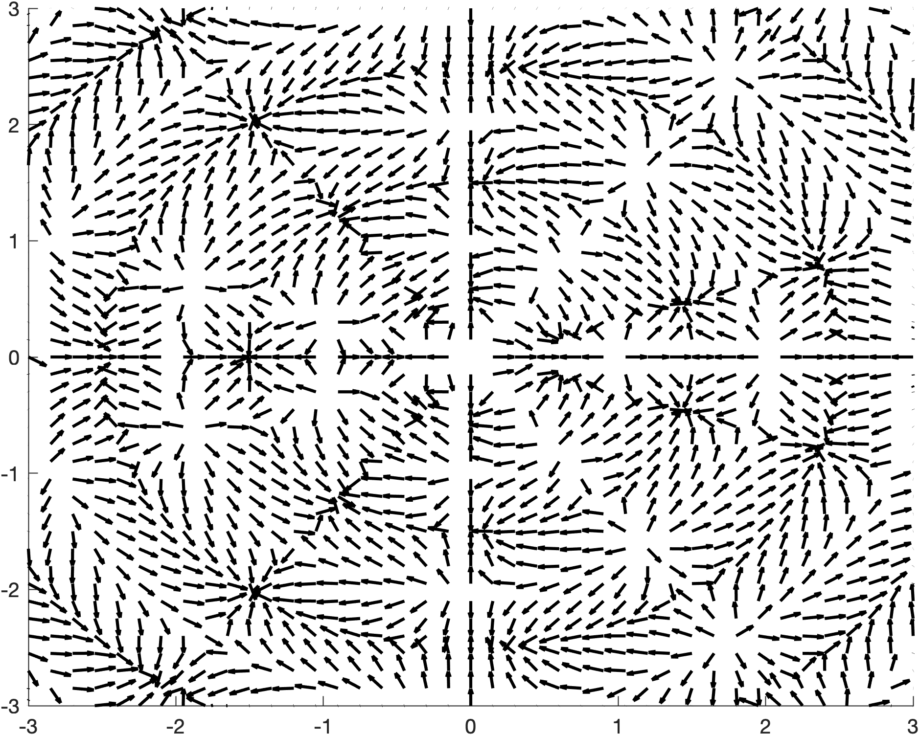
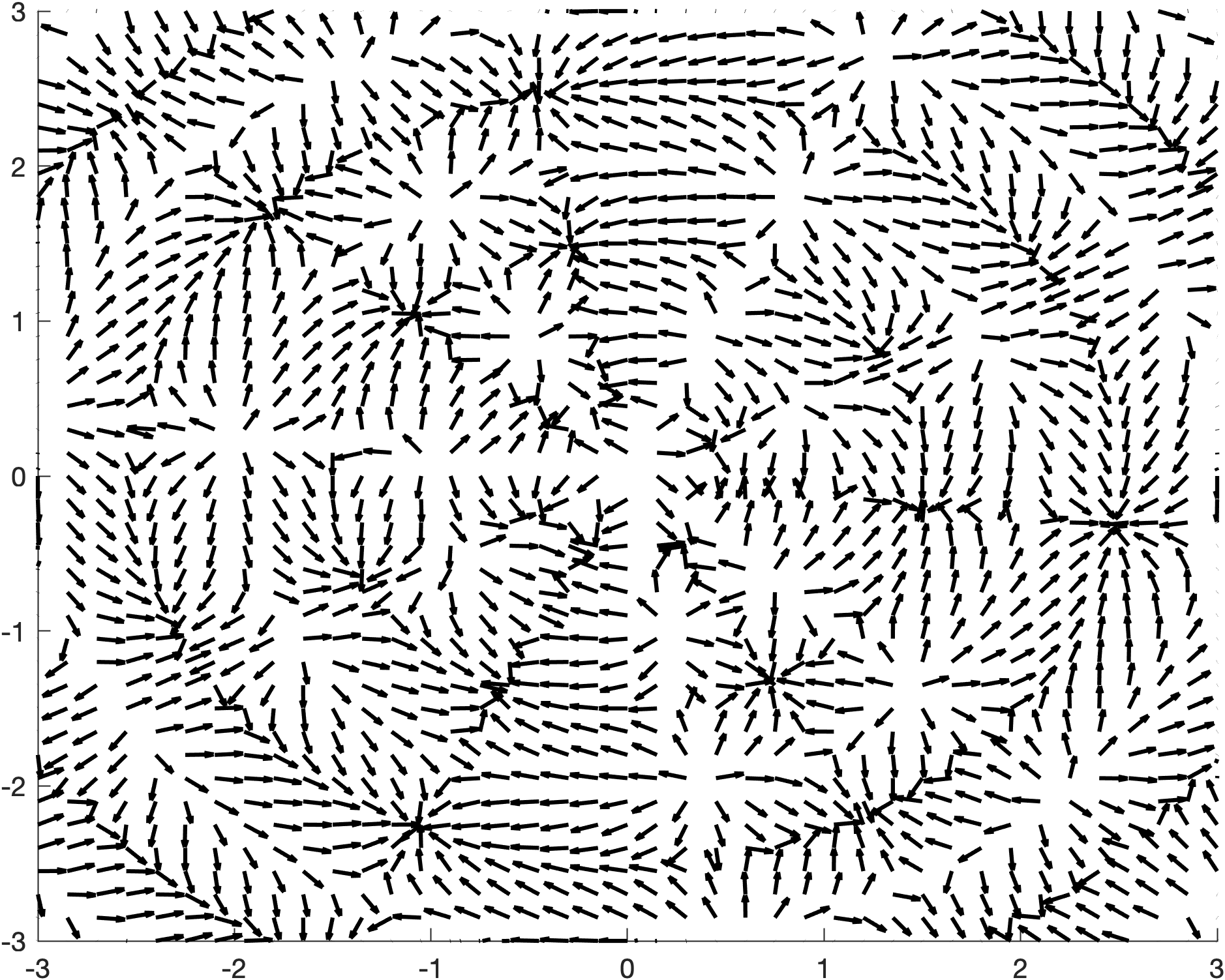
On we then define a time-dependent vector field by
| (3) |
Since the vector field extends continuously to by setting by . We call the radial part and the angular part of . The radial part is time-independent, determined by and radially symmetric, while the angular part is time-dependent, determined by and equivariant with respect to multiplication by real scalars.

We consider -periodic orbits of the vector field , i.e. solutions of . Note that, since for all , the constant map is a 1-periodic orbit of . From now on let us denote
| (4) |
The set may be empty, but by definition of .
In the next two lemmas, we classify all 1-periodic orbits of .
Lemma 2.1.
Proof.
We include the straightforward calculation here for the convenience of the reader. For the map is the constant orbit. Otherwise,
shows the claim. ∎
Lemma 2.2.
Assume . Let be a -periodic orbit for . Then there are and such that is a -fold iteration of , that is
Proof.
We, of course, assume that for all since otherwise is the constant orbit . Thus, it is convenient to use polar coordinates , i.e. . In polar coordinates, the vector field is given by
and transforms into
| (6) |
where the function satisfies for all and some .
Since is -periodic, the first equation in (6) implies by uniqueness of solutions of ODEs that is constant and , that is . In particular, .
It remains to consider the second equation in (6), that is for all . We recall that , , is a solution to the second equation in (6). Therefore, if for some , then for all by uniqueness of solutions of ODEs.
Thus, we now assume that for all . In fact, we may assume that for all and all since otherwise for some which again contradicts uniqueness. Now choose some and consider
| (7) | ||||
By our assumption we know that . Let us assume for now that . Since satisfies and since is a periodic function there exists with for all and we conclude from (7) that the difference grows at least as fast as , i.e. cannot be bounded from above. If we similarly conclude that shrinks at least as fast as and cannot be bounded from below.
We conclude that our assumption is wrong and therefore for some . In particular, , that is and therefore, is the -fold cover of . ∎
To see when Theorem 1.1 applies to the explicit family of 1-periodic orbits we first recall the definition of non-degeneracy.
Definition 2.3.
Let be a -periodic orbit of a (time-dependent) vector field on . Denote by , , the flow of . The periodic orbit is called non-degenerate if the linearized time--map does not have as an eigenvalue.
The following is an alternative characterization of non-degeneracy in terms of the vector field.
Lemma 2.4 ([AS22, Lemma 6.6]).
Let be a 1-periodic orbit of . For we consider the linear map
and denote by the fundamental system for , that is, the solution of
| (8) |
Then
holds and, in particular, is non-degenerate if and only if does not have as an eigenvalue.
Now we can characterize when an orbit is non-degenerate.
Lemma 2.5.
Fix and . The -periodic orbit is non-degenerate if and only if and .
Proof.
We will use the alternative characterization of non-degeneracy from Lemma 2.4. Since the notion of non-degeneracy is coordinate independent we work again in polar coordinates. From together with we conclude
Since is time-independent (and diagonal) its fundamental system is simply given by , i.e.
| (9) |
Therefore, is not an eigenvalue of if and only if and . ∎
3. 1-periodic delay orbits
Now we consider the delay differential equation
| (10) |
where and is as in (3), that is,
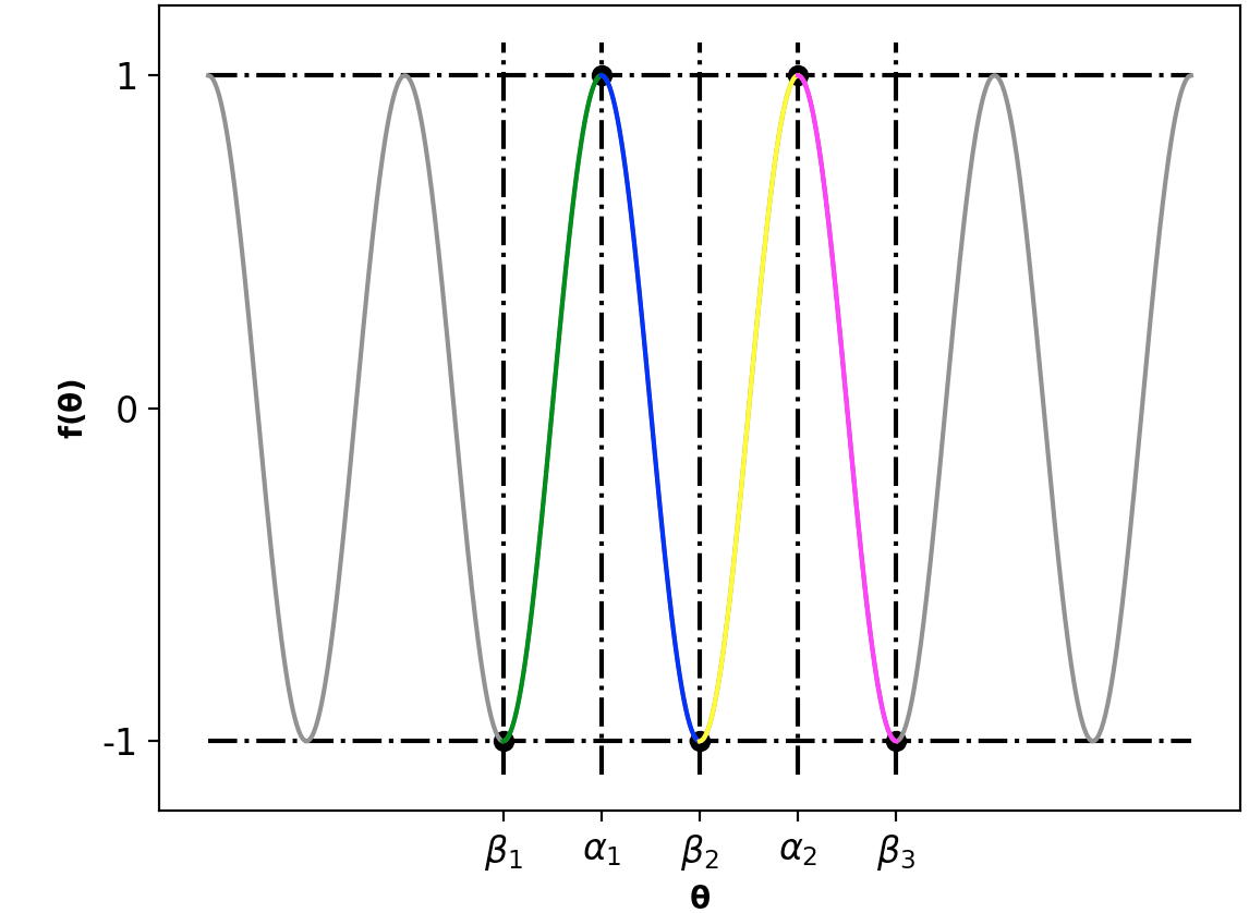
Since we require , the constant orbit also solves (10) for every value of . As opposed to the corresponding ordinary differential equation it is not clear (to us) how to construct or read off (periodic) delay orbits from the portrait of , e.g. Figure 1. We point out that, again opposed to solutions to the ODE, different delay orbits may agree at various times without agreeing globally. In particular, a delay orbit may run into the constant orbit and then out again.
Let us fix and . If and , then the orbit defined in Lemma 2.1 is non-degenerate by Lemma 2.5. Thus, Theorem 1.1 asserts that, for small enough , there is a unique -periodic solution of the delay equation (10) which is -close to the given orbit . At this point, however, we do not know what looks like. Moreover, if or then is a degenerate orbit and we cannot apply Theorem 1.1.
In Lemma 3.1 below we will show that the loop
where and are solutions to
| (11) | ||||
| (12) |
indeed solves the delay equation (10). We point out that for the choice of and recovers the (locally unique) solution to the corresponding ODE. In accordance with Theorem 1.1 we expect to find delay orbits -close to , at least for small delay . This translates into being close to and being close to .
Lemma 3.1.
Remark 3.2.
In Lemma 3.1 we do not require the delay to be small. We point out, however, that, depending on and , solutions of (11) resp. of (12) may neither exist nor be unique. Moreover, as long as and are solutions of (11) and (12) the loop is a -delay orbit. This does not require being close to some or being close to some . In fact, or is allowed in Lemma 3.1.
Proof of Lemma 3.1.
Remark 3.3.
As opposed to Lemma 2.2 we do not expect that there is a similar uniqueness statement for periodic delay orbits of the vector field .
4. Analyzing the family
We will now analyze the delay orbits arising for different choices of and and corresponding solutions of (11) and of (12).
We note that the 1-periodic delay orbit moves with constant angular speed on the circle of radius . In particular, we can recover from a single value, e.g. . Therefore, we choose to represent a family of 1-periodic delay orbits by the curve
| (14) |
From this explicit expression it is clear that is smooth if and smoothly depend on .
4.1. The non-degenerate case
We recall from Lemma 2.5 that the 1-periodic orbit of is non-degenerate if and only if for and for . In fact, non-degeneracy of , i.e. and , allows us to locally uniquely solve equations (11) and (12) as follows. For that first choose a local inverse
from an interval containing onto a neighborhood of . In particular, . Then, for small enough (more precisely, whenever ), we set
| (15) |
By construction, solves (11). Next, we abbreviate
and observe that the assumption for implies
Again, we choose a local inverse
from an interval containing to a neighborhood of , in particular , and set
| (16) |
which, by construction, solves (12).
For convenience let us assume that resp. are the maximal intervals on which the inverses resp. are well-defined.
Remark 4.1.
We collect a few conclusions.
-
(1)
If (not necessarily small) is such that and , we define resp. by (15) resp. (16). In particular, we then obtain a 1-periodic -delay orbit .
Moreover, the so defined maps and are continuous. They are smooth except for with or .
-
(2)
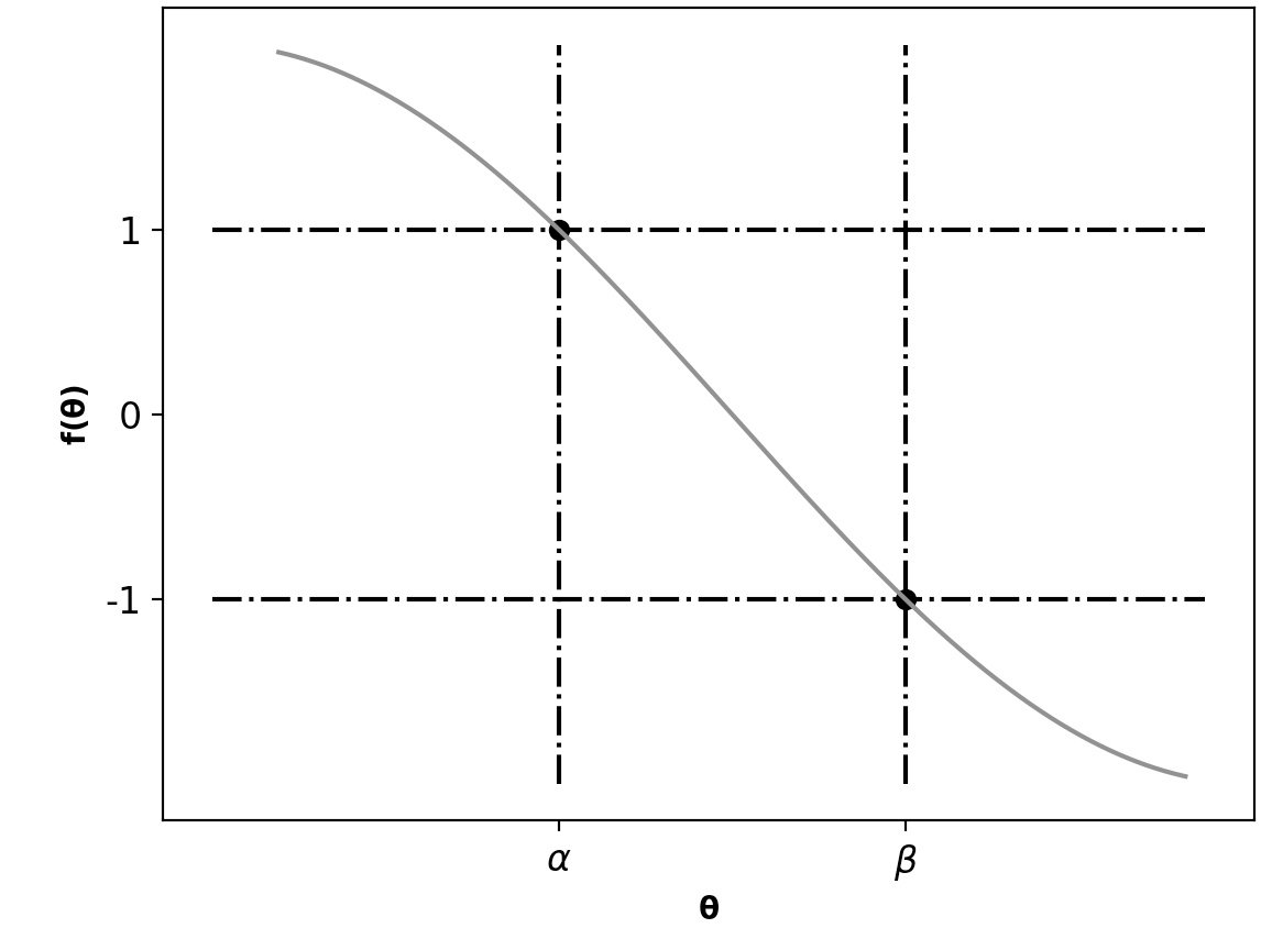
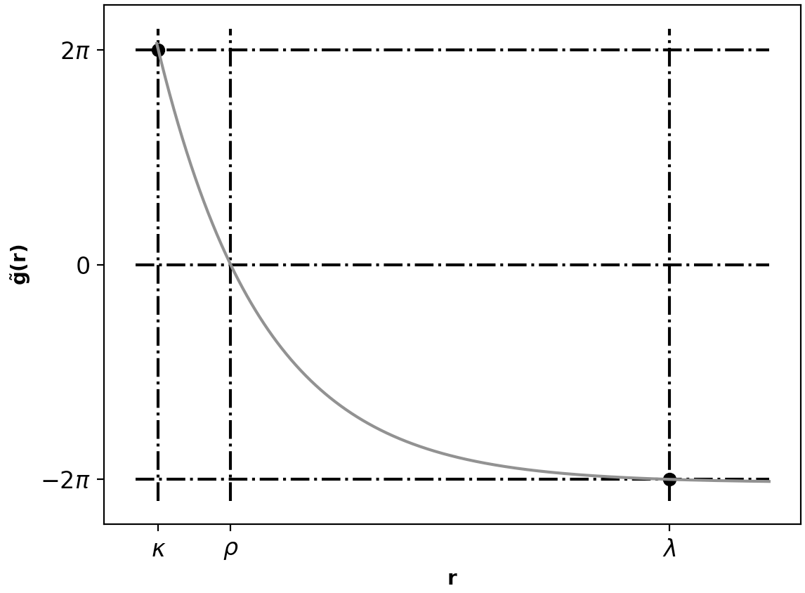
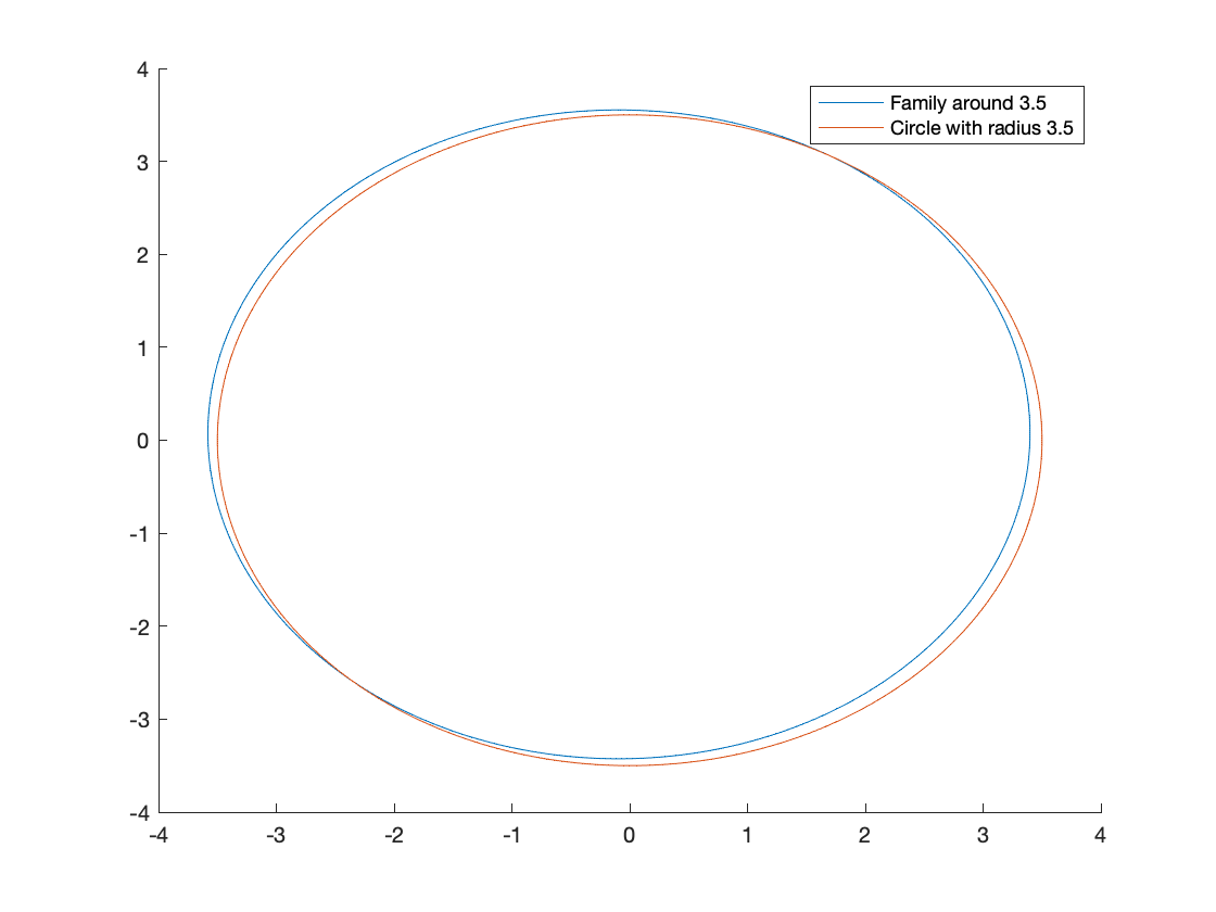
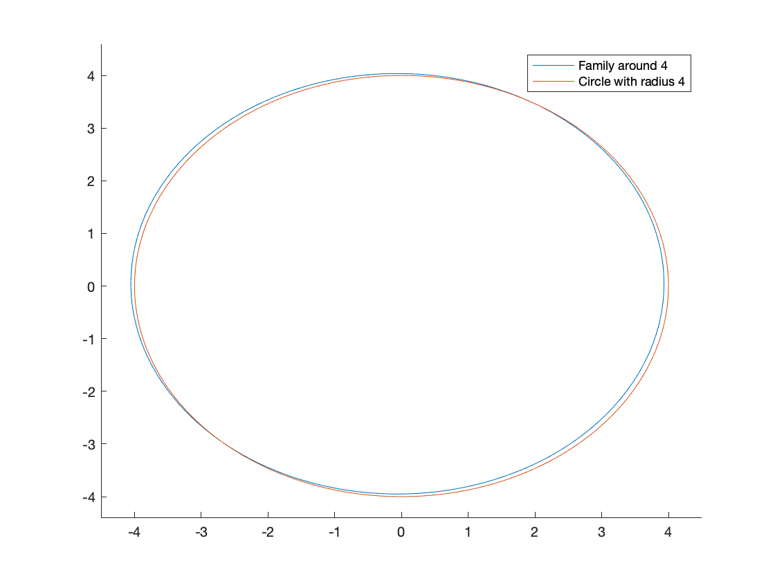
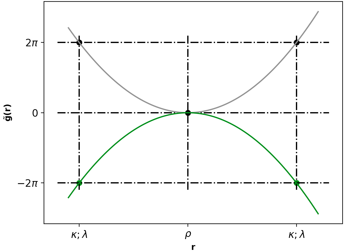
Sometimes and , see Figure (2) and Figure (3) below. In this case the maps and are defined for all . Moreover, they are -periodic in . Hence, in this case the -delay orbits , , actually form an -family.
More precisely, as runs through the value oscillates between , for , and , for , and similarly the value oscillates between , for , and , for .
Let us discuss possible cases a bit further.
-
(a)
We have if and only if there is some with and such that is strictly monotone on a segment in from to . In this case, the set from above is exactly this segment from to .
-
(b)
If we, in addition, know that , then the local inverse is smooth, implying that is smooth as well.
-
(c)
On the other hand, if is a non-degenerate local minimum (i.e. and ) with then we still have and we could proceed as above. On the other hand, we could also choose to continue the map by switching from the local inverse at to the local inverse of on “the other side” of , see Figure (6(a)).
-
(d)
Similarly, we have if and only if there are with , such that either or and is strictly monotone between and . The set is then exactly the interval between and . Again, implies that is smooth and thus so is . A similar discussion as above for is possible.
-
(e)
We call an -family smooth if both local inverse and are smooth functions, i.e. if and holds. This implies, that its associated curve is smooth.
-
(a)
-
(3)
If exists, then we can allow for , and hence may become , namely if or . In this case the family of -delay orbits contains the constant delay orbit at .
Without further assumptions on , it is not clear that extends continuously to and therefore it is also not clear how the local inverse behaves as the values approach . In particular, we can only continue the family beyond if and or if and .
We do point out, however, that, if is in , then admits a extension to , since .
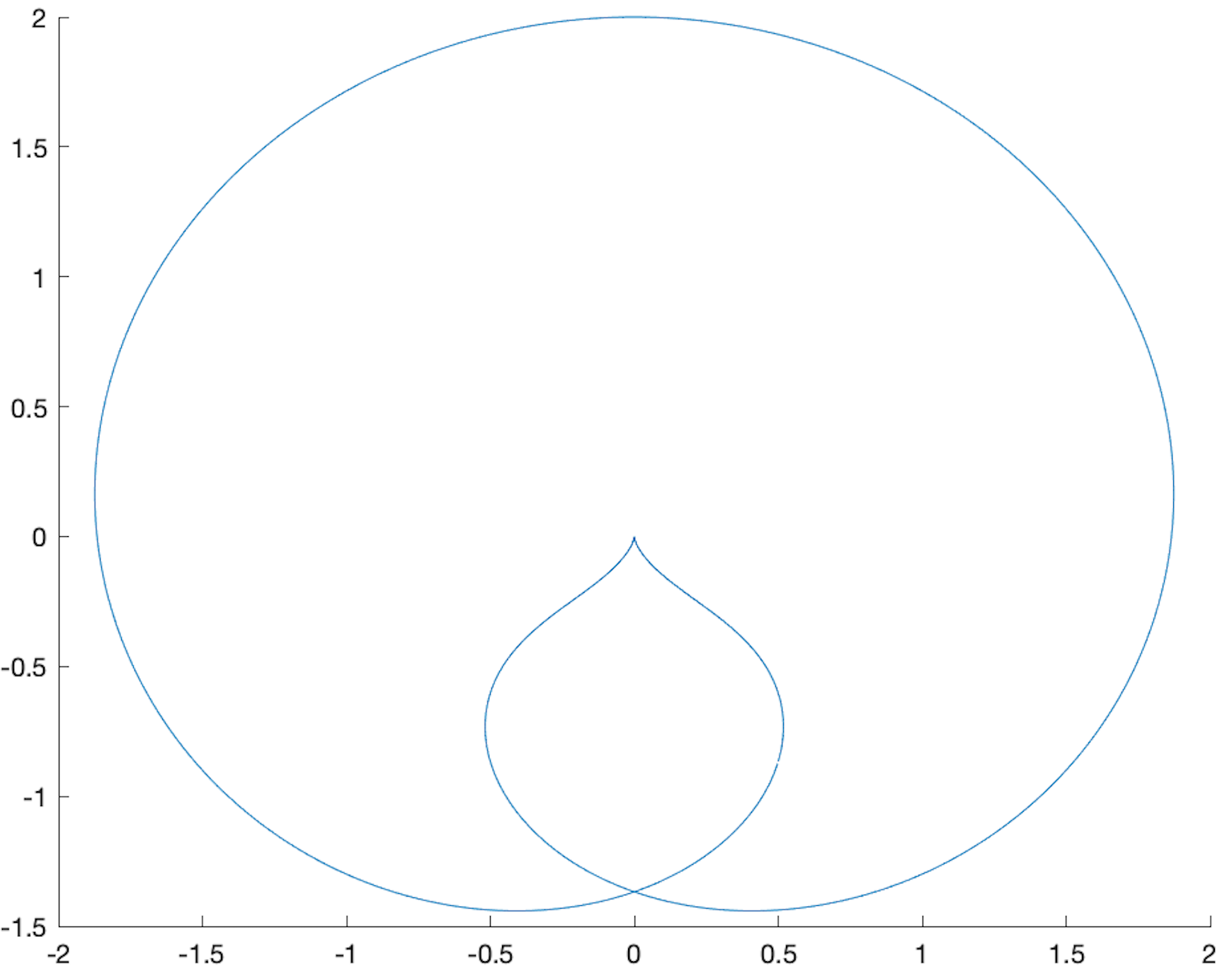
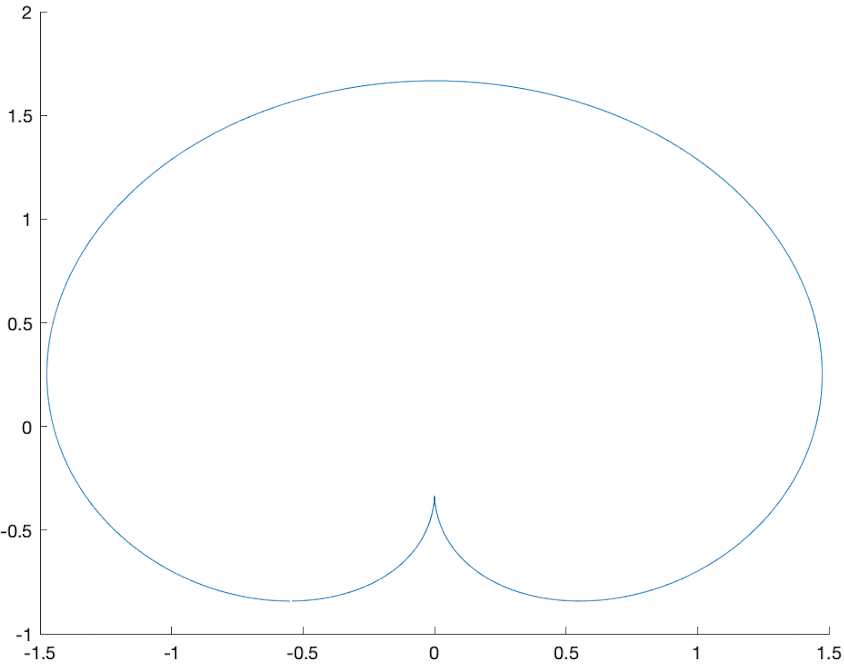
4.2. Cusps
Recall that we represent families of delay orbits by the curve in the plane given by , see (4) for details. In example plots of the curve often exhibit isolated cusps-type singularities, see Figure (4) and (5), meaning that if the derivative of has a zero at some then this is an isolated zero and there necessarily is a switch of direction of the normalized tangent vector to at . We are going to explore this further now. For that, we assume in this section that the maps and both are smooth.
Lemma 4.2.
The curve has only isolated singularities. More precisely, the condition implies that or .
Conversely, assume or . Then if one of the following holds:
-
(i)
,
-
(ii)
in case resp. in case .
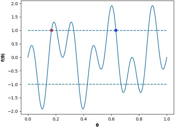
The dots mark the choices for
(red: , blue: ).
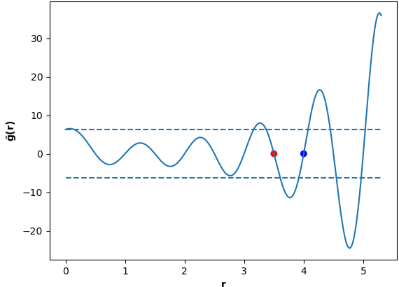
The dots mark the choices for
(red: , blue: ).
Proof.
We first discuss the condition . From
| (17) |
we conclude that is equivalent to
| (18) |
Let us analyze these two equations individually. Recalling the definition (16) of and that is a local inverse for leads to
| (19) |
and we conclude that is equivalent to or . In particular, we see that implies or .
Proposition 4.3.
Assume that . Then the curve necessarily has a cusp at , that is
| (22) |
I.e., the normalized tangent vector switches direction at .
Proof.
Since the maps and are smooth, so is and we use first order Taylor approximation of near , i.e.
| (23) |
for some function with . Therefore, the desired condition (22) holds, if we can show that . For this, we recall from the proof of Lemma 4.2 that
| (24) |
see equation (4.2). In particular, is equivalent to
| (25) |
Therefore, from
| (26) | ||||
we conclude that if and only if
| (27) |
is non-zero. We claim that the first term never vanishes. Indeed, using (16) we obtain
Now, Lemma 4.2 asserts that implies or . In either case the first summand in is non-zero and the second summand vanishes. This proves and therefore the Proposition. ∎
With the analysis from the proof above at hand, we make some simple observations about the occurrence of cusps.
Corollary 4.4.
If the plot shows a cusp then it is always of 180°, meaning that the curve runs in and out of the cusp in opposite directions.
Corollary 4.5.
Proof.
We have seen in Lemma 4.2 that if cusps appear then and condition (i) or (ii) in Lemma 4.2 need to hold. Recall from 2.(e) in Remark 4.1 that, by assumption, we have for all . If at both cusps condition (ii) in Lemma 4.2 is satisfied then clearly for some , a contradiction. On the other hand, if we assume that condition (i) holds for both choices of , that is, , then for some in between and in , another contradiction. See equation (19) for the derivative of . Therefore, for exactly one satisfying condition (i) and the other satisfies condition (ii). ∎
4.3. The degenerate case
Assume now that the 1-periodic orbit (without delay) is degenerate, that is for or for . Note that the latter one implies . Similarly, has a maximum / minimum / saddle in if and only if does.
Next, following the construction of and from Section 4.1 and the ansatz we will point out similarities and difference in the degenerate cases.
- •
-
•
If has a local minimum in then there is no solution of (11) for . Therefore we cannot find delay orbits using the ansatz .
-
•
If has a local maximum in , then there are two different choices for a local inverse of near . This yields one solution for smaller than (and close to) and one solution for larger than (and close to) . For both solutions, is close to . In particular, we obtain two families of delay orbits meeting in for . They are not smooth for .
-
•
Similarly, if attains a local minimum in with then there are two different local inverses of near with values around . This implies that there are two families of delay orbits intersecting in the -delay orbit . We are not aware of a suitable definition of non-degeneracy for delay orbits similar to Definition 2.3, but this observation suggests that should be called degenerate if . Of course, here may be replaced by any element in .
-
•
Combining for with equation (12) we see that, if attains a local minimum resp. local maximum in , then our ansatz works only for resp. for .
-
•
Similar to the case that attains a local minimum in are the cases that attains a local minimum in or a local maximum in . In these cases, there are two different choices for a local inverse of near with values around or near with values around respectively. Hence there are two families of delay orbits meeting in the -delay orbit or in the -delay orbit , respectively. Again, the orbits and should be called degenerate. Also, again we may add to in this discussion.
5. Gluing families
We have seen in Section 4.3 that sometimes two families of delay orbits of the form meet in a degenerate orbit without delay, i.e. modulo or in a (degenerate) -delay orbit with , or modulo . More precisely:
-
•
if attains a local maximum in with .
-
•
if attains a local minimum in with .
-
•
if attains a local minimum in with or a maximum in with .
The two families then correspond to the two different choices of local inverse or “to the left” and or “to the right” of the respective extremum, which result in different solutions , to equations (11) and (12).
In this section, we look at two specific classes of functions and for which explicit computations are possible and which lead to interesting examples. In Section 5.1 we have a closer look at a particularly symmetric degenerate example coming from trigonometric functions where all extrema occur. We will see that it makes sense to glue the resulting families to each other in different ways and that we get very symmetric families of delay orbits from this glueing. After that, in Section 5.2, we repeat the procedure for polynomial functions. The same glueing can of course be performed in examples with less symmetry.
5.1. Trigonometric and
We fix a positive integer and choose and as the following trigonometric functions.
| (28) | ||||
| (29) |
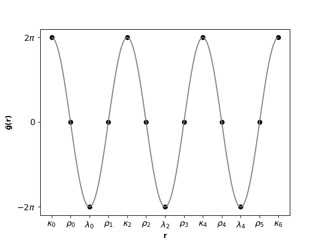
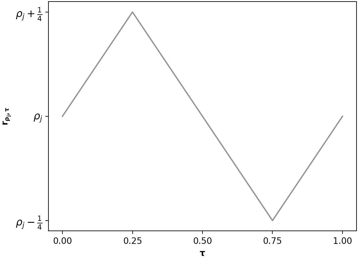
In the notation from above we have with , , and with , . For we have infinite sets of zeroes , maxima and minima , see Figure 7. Note that we label maxima and minima by even numbers only. Then we have the following inequalities for between zeroes, maxima and minima of :
Near each maximum of , we have two choices for the local inverse of . The inverse to the left of
and the inverse to the right of
For we have near each zero a local inverse which is, for even , given by
and for odd by
Near the extrema of we can choose between the local inverse to the left and the local inverse to the right. These are related to the other local inverse by and on the overlap of their respective domain of definition. To the left of a maximum , , we have the local inverse (if ), to the right of we have . To the left of a minimum , , there is , to the right of there is .
All these local inverses are not smooth at the boundaries of the intervals of definition since their derivatives blow up. Therefore, if we use these inverses to define -families of delay orbits via (15), (16) and (13) in Section 4.1, we obtain -families which are not smooth in due to , and not smooth in due to .
However, if we switch at each , , and from the local inverse to the left to the local inverse to the right (or vice versa) as discussed at the beginning of this section we can define smooth families after all. Concretely, let us define solutions resp. ( and indicates “left to right” and vice versa) to (11) by
respectively by
Note that these families no longer form -families but are parametrized over intervals. However, families for and agree in their ends, that is
where . Hence we obtain “bigger” families by glueing the ends of consecutive “small” families. In this way, we obtain two distinct families of solutions for equation (11) given as
and
Both these solutions are -periodic, so we can think of them as parameterized by . This reflects the fact that we started with a periodic function .
Note that the corresponding two families of delay orbits do not depend on a particular choice of anymore, instead, each family runs through every point in consecutively. We arbitrarily chose to start at for for both solutions.
Similarly, we proceed to define smooth families and of solutions to (12). First, use the formula
from (16) for the different , . Since this yields continuous, piecewise affine linear functions with and slope switching between and at , see Figure 8.
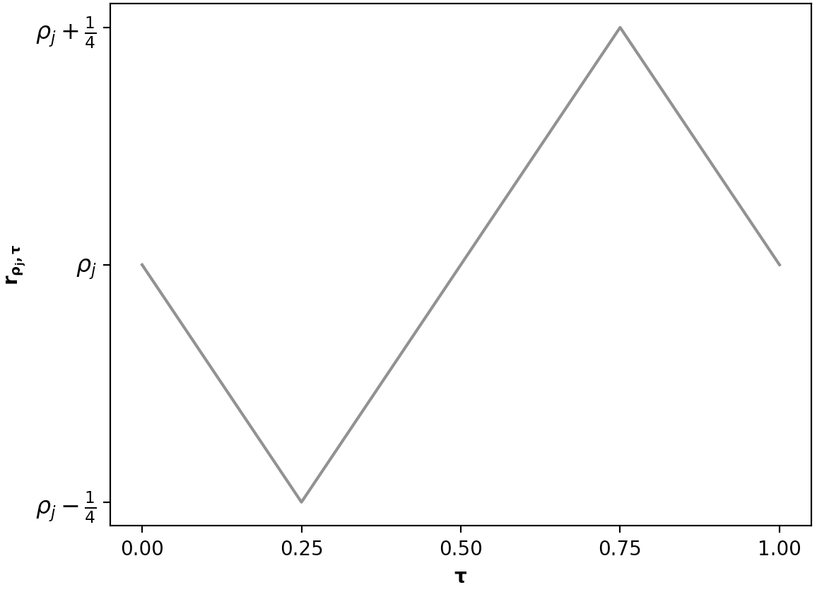
Then we can proceed and patch together the pieces for adjacent . This would yield -many affine linear (in particular, smooth) maps (of slope ) resp. (of slope ). However, the various only differ by a shift from each other, stemming from the choice . Therefore, we prefer to define families and which do not depend on a particular point in but instead run through all points of consecutively again. We arbitrarily choose to let the -family pass through at and the -family through at . This gives the following explicit expressions.
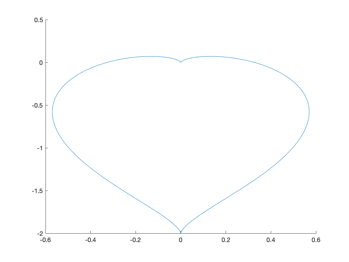
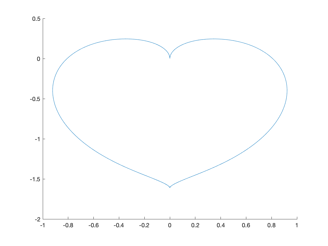
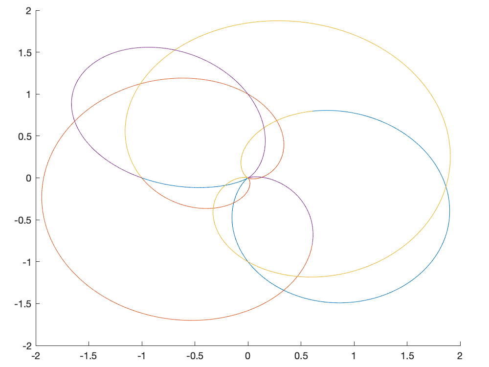
Finally, to define families of periodic delay orbits, we can now combine and with and resulting in four different families , parametrized by or respectively. Figure 9 shows the four curves for . For plotting reasons, we arbitrarily cut off the families of radii at .
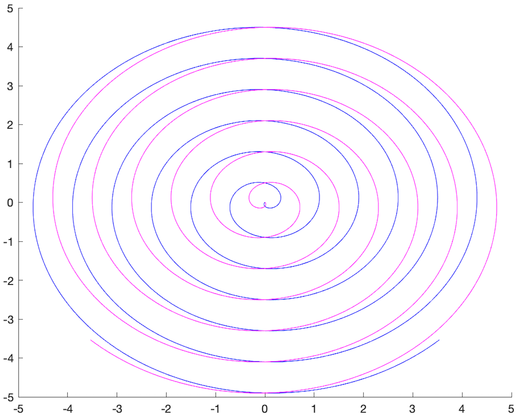
and (magenta) with
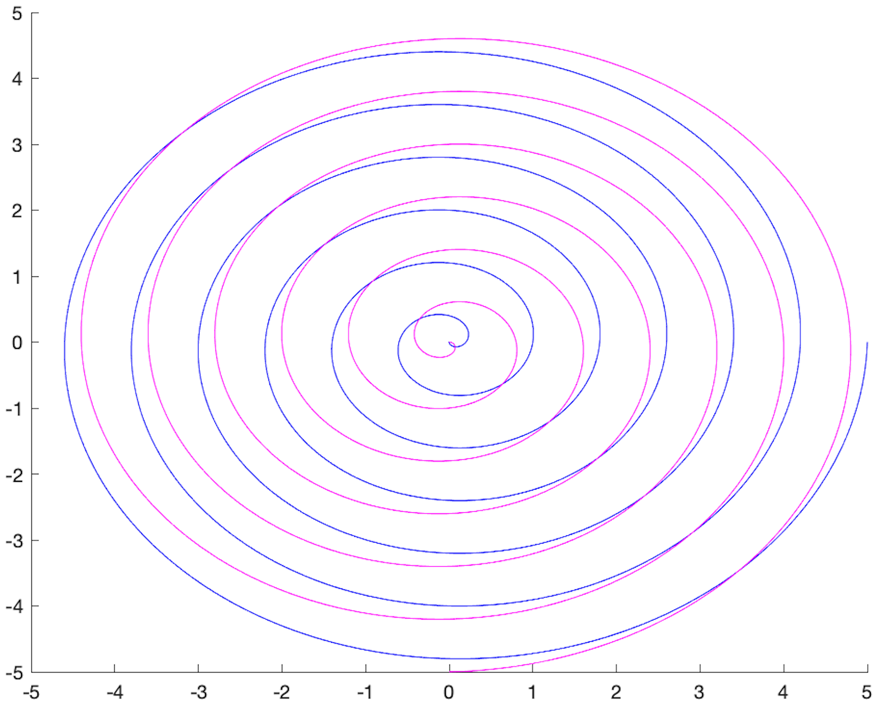
and (magenta) with
5.2. Polynomial and
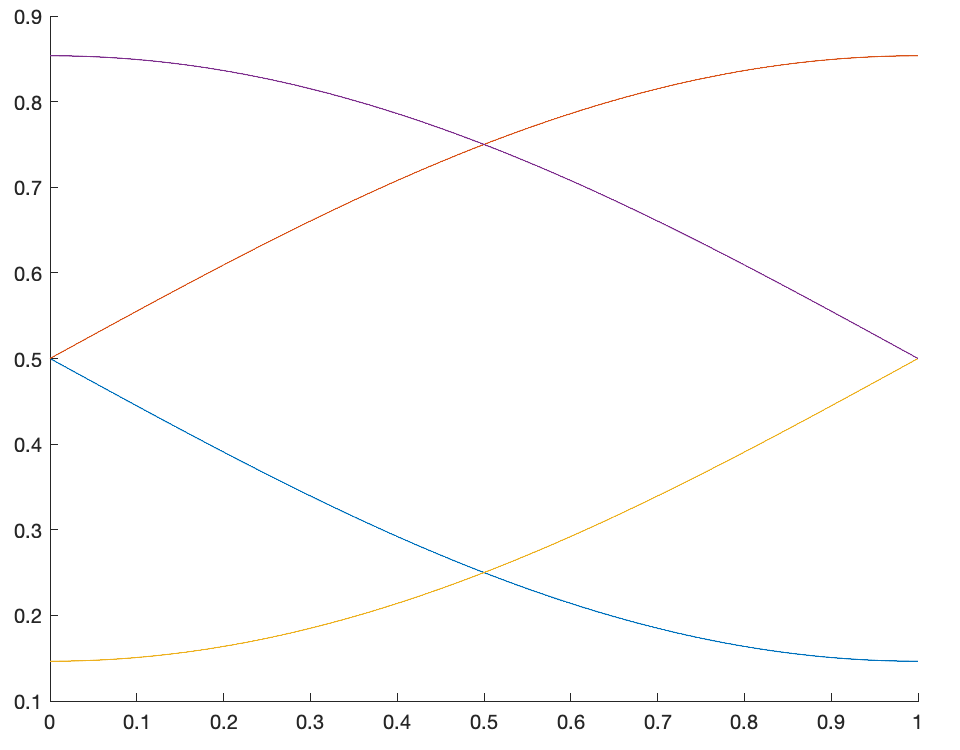
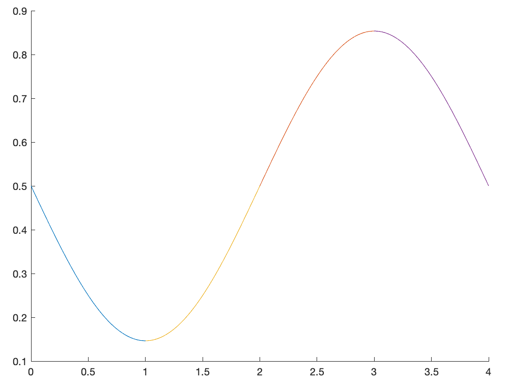
To showcase the above procedure in another example we consider
Clearly, and thus (12) leads to
From the expression for , we see that we will have four distinct local inverses. These local inverses meet at the minima given by and the maximum at . We denote the local inverses relative to their position to the two minima in resp. by
Again, each of these local inverses on its own would not lead to a smoothly parameterized family of delay orbits. This can be seen from the kinks in Figure (10(b)) which appear when switching between the red and violet arcs resp. the yellow and blue arcs at .
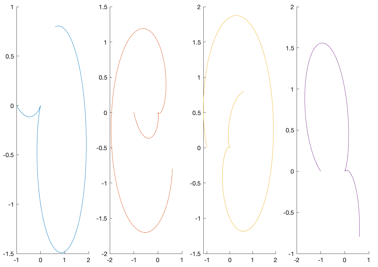
However, this problem can be dealt with in the same manner as before, namely by combining the local inverses appropriately. We define the two left-to-right solutions by
and
The two right-to-left solutions are
and
Since , we can combine these into one smooth -family
Any other cyclic permutation just gives another parameterization of the same family. The resulting is shown in figure (11).
References
- [AS22] Peter Albers and Irene Seifert. Periodic delay orbits and the polyfold implicit function theorem. Comment. Math. Helv., 97(2):383 – 412, 2022.
- [DGLW95] Odo Diekmann, Stephan A.van Gils, Sjoerd M.V. Lunel, and Hans-Otto Walther. Delay Equations. Springer New York, 1995.
- [FW21] Urs Frauenfelder and Joa Weber. The shift map on Floer trajectory spaces. J. Symplectic Geom., 19(2):351 – 397, 2021.
- [HWZ21] Helmut Hofer, Krzysztof Wysocki, and Eduard Zehnder. Polyfold and Fredholm Theory. Ergebnisse der Mathematik und ihrer Grenzgebiete. Springer, 2021.
- [Sei22] Irene Seifert. Polyfold methods for the study of periodic delay orbits. PhD thesis, Universität Heidelberg, 2022.