TagCLIP: Improving Discrimination Ability of Open-Vocabulary Semantic Segmentation

Abstract

Recent success of Contrastive Language-Image Pre-training (CLIP) has shown great promise in pixel-level open-vocabulary learning tasks. A general paradigm utilizes CLIP’s text and patch embeddings to generate semantic masks. However, existing models easily misidentify input pixels from unseen classes, thus confusing novel classes with semantically-similar ones. In our work, we disentangle the ill-posed optimization problem into two parallel processes: one performs semantic matching individually, and the other judges reliability for improving discrimination ability. Motivated by special tokens in language modeling that represents sentence-level embeddings, we design a trusty token that decouples the known and novel category prediction tendency. With almost no extra overhead, we upgrade the pixel-level generalization capacity of existing models effectively. Our TagCLIP (CLIP adapting with Trusty-guidance) boosts the IoU of unseen classes by 7.4% and 1.7% on PASCAL VOC 2012 and COCO-Stuff 164K.

1 Introduction

The long-term and challenging purpose of deep learning [28, 10] is to approach human-level perception. Humans understand scenes in an open-vocabulary manner, typically in multiple ways including vision, language, sound, etc. Following this principle, pioneers proposed open-vocabulary algorithms in multiple computer vision tasks, including classification [25], semantic segmentation [19, 35, 40], object detection [11, 13] etc.

Although the literature of works has achieved remarkable results [22, 27, 3, 4], deep learning models are found easily fail to generalize to novel classes that are unavailable during training. To improve the generalization ability of vision networks, previous researchers leveraged the recent advance in vision-language learning models, e.g., CLIP [26], which learns rich multi-media features from a billion-scale image-text dataset.

With the superior ‘openness’ from web-scale image-text pair, vision-language models have been utilized in various manners [35, 19, 40]. Pioneers proposed two-stage approaches: first generate class-agnostic proposals and then leverage pre-trained vision-language models like CLIP [26] to perform open-vocabulary classification. More recent approaches [40] boost both the performance and speed of open-vocabulary semantic segmentation by proposing one-stage approaches: they adopt a post-CLIP lightweight decoder that matches text prompts and image embeddings to generate segmentation maps.

However, investigating visualization results as shown in Fig. 1, we find that even the current SoTA [40] struggles with pixels from novel classes and overfits them with seen semantics, like ‘cloud’ with ‘sky-other’, and ‘playingfield’ with ‘dirt’, etc. To address this issue, we propose to disentangle the ill-posed optimization problem into two processes: one performs semantic matching individually, and the other determines prediction reliability that discriminates novel classes.

A straightforward solution is to apply outlier detectors [17] before feeding inputs to the downstream networks. Nevertheless, an additional serial outlier detection stage inevitably doubles time and storage costs. In our work, we propose a novel framework, as shown in Fig. 2. Motivated by special tokens in language modeling that represents sentence-level embeddings [12, 31, 8], we design an additional trusty token that denotes the prediction tendency that discriminates known and novel categories.

We concatenate the trusty token with original classes and optimize it with our Trusty Learner on the inter-category relationship, which performs the trustworthy judgment with semantic matching in parallel. With almost no extra overhead, our TagCLIP (CLIP adapting with Trusty-guidance) well discriminates unseen classes from known categories. As shown in Fig. 1, compared with current SoTA, our proposed approach correctly separates the hard unknown classes, including ‘clouds’,‘playing field’, ‘grass’, etc. More visualization results are in Sec. 4.2.

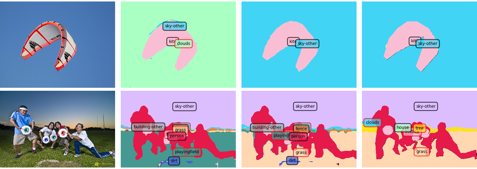
Figure 1: Visualization of segmentation results on COCO-Stuff 164K. Four columns from left to right represent (a) Original testing images; (b) Results of current SOTA [40]; (c) Results of TagCLIP; (d) Ground truth. The tags with borders in black and red denote seen and unseen classes separately.

We perform extensive experiments to evaluate our proposed approach. Our method boosts the Intersection over Union (IoU) of unseen classes by 7.4% on PASCAL VOC 2012 and by 1.7% on COCO-Stuff 164K, as shown in Tab. 2. In the cross-dataset setting, our method improves the SoTA’s performance by 1.4% from COCO-Stuff 164K to PASCAL Context, shown in Fig. 6. We also provide the results trained with full labels in Tab. 5. It illustrates that our method improves the upper bound of open-vocabulary segmentation results by 1.9% on PASCAL VOC 2012 and by 0.4% on COCO-Stuff 164K.

To sum up, the contributions of our method are as follows:

1. We disentangle the ill-posed optimization into two parallel processes: one judges reliability to improve discrimination, and another performs semantic matching individually.

2. We design a trusty token and optimize it with Trusty Learner, which extracts the known and novel category prediction tendency with almost no extra overhead.

3. Our TagCLIP shows competitive performance in extensive open-vocabulary semantic segmentation tasks, including inductive setting, transductive setting, and cross-dataset tasks, etc.

2 Related Works

Pretrained Vision Language Model

Large-scaled pre-trained vision language models [15, 18, 26, 30] combined image representation and text embeddings have achieved impressive performance on multiple downstream tasks, including image retrieval [21], visual question answering [16], visual referring expression [32], dense prediction [39], etc. Among them, CLIP [26] is one of the most widely-used vision-language models. CLIP is trained via contrastive learning on a billion-scale text-image dataset and shows its powerful generalization ability on various tasks [35, 19, 40].

Zero-shot Semantic Segmentation

Semantic segmentation is an essential task in computer vision [22]. Pioneers directly addressed segmentation with per-pixel classification algorithms [22, 29, 34, 37, 38]. Followers improved them by decoupling mask generation with semantic classification [5, 6, 36]. When segmenting pre-defined closed categories, both principles have achieved significant progress. Nevertheless, when inferring novel classes inaccessible from training, normal approaches perform poorly. Thus, zero-shot semantic segmentation has been a challenging task, whose key is to segment unseen categories via training on only known classes. Mainstream works [33, 2, 14, 7, 1, 24] focus on improving the generalization ability from seen to novel categories.

Open-Vocabulary Semantic Segmentation.

Inspired by the powerful generalization ability of CLIP [26], researchers have leveraged it for open-vocabulary semantic segmentation. Early researchers proposed a two-stage paradigm [35, 19]: they first train a proposal generator and then utilize CLIP for pixel-level classification. The latest works [40] simplify this process by proposing a one-stage approach that adds a lightweight transformer after CLIP as a decoder for segmentation. However, existing approaches still struggle with pixels from novel classes and overfit them with seen semantics. In our work, we proposed a novel framework called TagCLIP to improve discrimination ability, as shown in Fig. 2.

3 Method

Our method follows the literature of open-vocabulary semantic segmentation [33]. Its task is to train the model on only part of the classes but learned the capacity of segmenting both known classes and novel classes. During training, the pixel annotations of unseen classes $C_{U}$ are masked and the seen part $C_{S}$ remains. During inference, the model is tested on the raw dataset with $C=C_{U}\cup C_{S}$.

In this section, we first introduce the framework of our proposed method (Sec. 3.2) and then propose the included techniques in training (Sec. 3.3) and testing (Sec. 3.4) stages.

3.1 Preliminary

Recent work [40] has proposed an efficient one-stage open-vocabulary semantic segmentation pipeline. In the one-stage framework, a vanilla light-weight transformer [36] after the CLIP [26] matches class tokens and image embeddings extracted from pre-trained CLIP. To be more specific, the process of the one-stage pipeline is as follows:

Firstly, we leverage deep prompt tuning to adapt CLIP [26] to our target dataset. Then, we extract CLIP’s text tokens as $\mathbf{T}=[\mathbf{t}_{1},\mathbf{t}_{2},\dots,\mathbf{t}_{C}]\in\mathbb{R}^{C\times d}$ and class tokens of CLIP’s image encoder as $\mathbf{H}=[\mathbf{h}_{1},\mathbf{h}_{2},\dots,\mathbf{h}_{C}]\in\mathbb{R}^{N\times d}$, where $C$ is the number of classes and $d$ is CLIP’s feature dimension. Next, the inputs for transformer decoder [36] are:

$$\mathbf{\hat{t}}={\rm concat}[\mathbf{t}\odot\mathbf{h},\mathbf{t}],$$ (1)

where $\odot$ is the Hadamard product. Then linear projections $\phi$ are applied to generate $\mathbf{Q}(query)$, $\mathbf{K}(key)$ and $\mathbf{V}(value)$ as:

$$\mathbf{Q}=\phi_{q}(\mathbf{\hat{T}})\in\mathbb{R}^{C\times d},\mathbf{K}=\phi_{k}(\mathbf{E})\in\mathbb{R}^{N\times d},\mathbf{V}=\phi_{v}(\mathbf{E})\in\mathbb{R}^{N\times d}.$$ (2)

where $\mathbf{E}=[\mathbf{e}_{1},\mathbf{e}_{2},\dots,\mathbf{e}_{N}]\in\mathbb{R}^{N\times d}$ are the patch embeddings of the image encoder. Finally, the semantic masks $\mathbf{M}_{S}$ are calculated by:

$$\mathbf{M}_{S}={\rm Sigmoid}(\frac{\mathbf{Q}\mathbf{K}^{T}}{\sqrt{d}})\in\mathbb{R}^{N\times L},$$ (3)

where $\sqrt{d}$ is the scaling factor. The shape of the $\mathbf{M}_{S}$ is $N\times L$, and it can be further reshaped to $N\times\frac{H}{P}\times\frac{W}{P}$, where $P$ is the patch size.

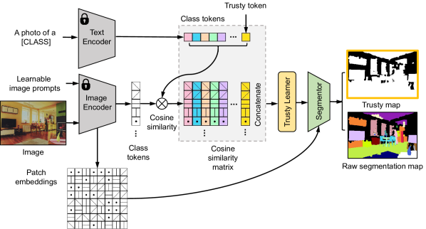
Figure 2: The framework of our TagCLIP. First, we input images and text prompts into CLIP and concatenate a learnable trusty token with CLIP’s text tokens. Then, we match the concatenated tokens with image tokens and input the similarity matrix into our proposed Trusty Learner. Next, we perform a segmentor [36] to generate two maps: the trusty map and the raw segmentation map.

3.2 Our Framework

Learnable Trusty Token.

Starting from the investigations in Fig. 1, existing methods [40, 9, 35] easily misclassify input pixels from unseen classes. To address this issue, we propose to disentangle the ill-posed baseline into two processes: one performs semantic matching individually, and the other simultaneously judges prediction reliability to improve discrimination. We denote an additional trusty token as $\mathbf{t}_{A}\in\mathbb{R}^{1\times d}$ to reflect the known and novel category prediction tendency.

We concatenate $\mathbf{t}_{A}$ with the text tokens $\mathbf{T}=[\mathbf{t}_{1},\mathbf{t}_{2},\dots,\mathbf{t}_{C}]\in\mathbb{R}^{C\times d}$ to get $\mathbf{T}^{\prime}=[\mathbf{t}_{1},\mathbf{t}_{2},\dots,\mathbf{t}_{C},\mathbf{t}_{A}]\in\mathbb{R}^{(C+1)\times d}$, where $C$ is the number of classes and $d$ is the feature dimension of CLIP.

Trusty Learner.

Following [40] on matching the new text tokens $\mathbf{T}^{\prime}$ with class tokens of CLIP’s image encoder as $\mathbf{H}=[\mathbf{h}_{1},\mathbf{h}_{2},\dots,\mathbf{h}_{C}]\in\mathbb{R}^{C\times d}$, we compute their cosine similarity matrix and concatenate it with $\mathbf{T}^{\prime}$:

$$\mathbf{\hat{t}}={\rm concat}[\mathbf{t^{\prime}}\odot\mathbf{h},\mathbf{t}]\in\mathbb{R}^{(C+1)\times 2d},$$ (4)

where $\odot$ is the Hadamard product. To capture the inter-relationship between CLIP’s text tokens and inserted trusty tokens, we propose the Trusty Learner module. It constitutes a linear projection, a multi-head attention block with a shortcut, and a normalization layer, as shown in Fig. 3. The linear transformation firstly aligns the dimension from $2d$ to $d$. Then $\mathbf{\hat{T}}$ is fed into the Trusty Learner and provides the output formulated by:

$$\mathbf{\tilde{T}}={\rm Norm}({\rm Softmax}(\frac{\mathbf{\mathbf{\hat{T}}}\mathbf{\mathbf{\hat{T}}}^{T}}{\sqrt{d}})\mathbf{\mathbf{\hat{T}}}+\mathbf{\hat{T}})\in\mathbb{R}^{(C+1)\times d},$$ (5)

where $d$ is the feature dimension of CLIP. Experiments in Sec. 4.1 shows that our proposed Trusty Learner is effective for instructing the trusty token $\mathbf{t}_{A}$.

Trusty Map Generation.

Inspired by the researches of [36, 40], we leverage the Attention-to-Mask (ATM) block to generate semantic segmentation maps. As the structure shown in Fig. 3, the inputs are projected by $\phi$ to form query ($\mathbf{Q}$), key ($\mathbf{K}$) and values ($\mathbf{V}$) as:

$$\mathbf{Q}=\mathbf{\tilde{T}}\in\mathbb{R}^{(C+1)\times d},\mathbf{K}=\phi_{k}(\mathbf{E})\in\mathbb{R}^{N\times d},\mathbf{V}=\phi_{v}(\mathbf{E})\in\mathbb{R}^{N\times d},$$ (6)

where $\mathbf{E}=[\mathbf{e}_{1},\mathbf{e}_{2},\dots,\mathbf{e}_{N}]\in\mathbb{R}^{N\times d}$ are the patch embeddings of CLIP’s image encoder. The semantic masks and predictions are calculated by:

$$\mathbf{Mask} ={\rm Sigmoid}(\frac{\mathbf{Q}\mathbf{K}^{T}}{\sqrt{d}})\in\mathbb{R}^{N\times L},$$ (7)

$$\mathbf{P} ={\rm Softmax}(\frac{\mathbf{Q}\mathbf{K}^{T}}{\sqrt{d}})\mathbf{V}\in\mathbb{R}^{N\times(C+1)},$$

where $\mathbf{Mask}\in\mathbb{R}^{N\times L}$ can be reshaped to $N\times\frac{H}{P}\times\frac{W}{P}$ and further to $H\times W$. By multiplying $\mathbf{Mask}$ and $\mathbf{P}$, we get the concatenated semantic segmentation maps $\mathbf{M}_{C}$ :

$$\mathbf{M}_{C}=\mathbf{M}_{S}\times\mathbf{P}\in\mathbb{R}^{(C+1)\times H\times W},$$ (8)

Note that we utilize ${\rm Sigmoid}$ as an activation function and the segmentation results of each class are independently generated. Therefore, $\mathbf{M}_{C}\in\mathbb{R}^{(C+1)\times H\times W}$ can be split into the trusty map $\mathbf{M}_{A}\in\mathbb{R}^{C\times H\times W}$ and raw semantic segmentation $\mathbf{M}_{R}\in\mathbb{R}^{1\times H\times W}$. We will introduce how to train and infer the maps next.

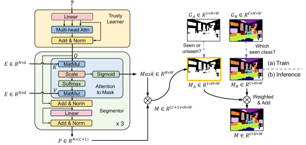
Figure 3: The Trusty Learner contains a linear projection, a multi-head attention block with a shortcut, and a normalization layer. The segmentor contains three layers. Each layer constitutes an Attention-to-Mask block [36] and a linear projection, both with shortcuts and normalization layers. The output of the segmentor is $\mathbf{M}_{C}\in\mathbb{R}^{(C+1)\times H\times W}$, which can be split into the trusty map $\mathbf{M}_{A}\in\mathbb{R}^{C\times H\times W}$ and raw semantic segmentation $\mathbf{M}_{R}\in\mathbb{R}^{1\times H\times W}$. During training, we propose a binary mask $\mathbf{G}_{A}\in\mathbb{R}^{1\times H\times W}$ for the supervision of $\mathbf{M}_{A}$. During inference, the raw semantic segmentation $\mathbf{M}_{R}$ is weighted by $\mathbf{M}_{A}$ to generate the final segmentation map $\mathbf{M}\in\mathbb{R}^{C\times H\times W}$.

3.3 Training Stage

Pseudo Labels.

The training process is illustrated in Fig. 3(a). In order to supervise the learnable token $\mathbf{t}_{A}$, we create a pseudo map $\mathbf{G}_{A}\in\mathbb{R}^{1\times H\times W}$, with each pixel labeled 1 for seen class and 0 for the unseen class as:

$$\mathbf{G}_{A}(i,j)=\left\{\begin{matrix}0{\rm,if\,}\mathbf{G}_{R}(:,i,j)\in C_{U}\\ 1{\rm,if\,}\mathbf{G}_{R}(:,i,j)\in C_{S},\end{matrix}\right.$$ (9)

where $C_{U}$ and $C_{S}$ are unseen and seen classes. $\mathbf{G}_{R}\in\mathbb{R}^{C\times H\times W}$ is the ground truth. In this way, although the model has no idea which unseen category the pixel is from, it discriminates unseen classes from known contexts. It has been experimentally demonstrated in Tab. 1 that our design effectively improve the generalization ability to novel domain.

Losses.

For training the Trusty Learner, the loss $\mathcal{L}_{A}$ is defined as:

$$\mathcal{L}_{A}=\mathcal{L}_{dice}(\mathbf{M}_{A},\mathbf{G}_{A}),$$ (10)

where $\mathcal{L}_{dice}$ is the dice loss [23, 40], $\mathbf{M}_{R}$ is the trusty map, and $\gamma$ is the weight of our loss. Integrated with the parallel branch that conducts semantic matching of open-vocabulary segmentation [40], the overall loss during training is:

$$\mathcal{L} =\mathcal{L}_{cls}+\mathcal{L}_{mask}+\gamma\mathcal{L}_{A},$$ (11)

$$=\mathcal{L}_{cls}+\alpha\mathcal{L}_{focal}(\mathbf{M}_{R},\mathbf{G}_{R})+\beta\mathcal{L}_{dice}(\mathbf{M}_{R},\mathbf{G}_{R})+\gamma\mathcal{L}_{dice}(\mathbf{M}_{A},\mathbf{G}_{A}),$$

where $\{\mathcal{L}_{cls},\mathcal{L}_{focal},\mathcal{L}_{dice}\}$ are the Binary Cross Entropy (BCE) loss, focal loss [20] and dice loss [23] with ${\rm Sigmoid}$ as activation function. $\mathbf{M}_{A}$ and $\mathbf{M}_{R}$ are the trusty map and raw semantic segmentation map. $\{\alpha,\beta,\gamma\}$ are weights of losses. We denote $\{\alpha,\beta,\gamma\}$ as $\{20,1,10\}$. More details are in Sec. 4.1.

3.4 Inference Stage

The inference process is illustrated in Fig. 3(b). To make further use of the trusty map $\mathbf{M}_{A}$, we utilize $\mathbf{M}_{A}$ to weigh the confidence of the raw segmentation map $\mathbf{M}_{R}$. Each value $\mathbf{M}_{A}(i,j)$ in $\mathbf{M}_{A}$ represents the possibility of the pixel $(i,j)$ from seen classes and $(1-\mathbf{M}_{A}(i,j))$ from novel categories. Consequently, we generate our final segmentation map $\mathbf{M}$ by

$$\mathbf{M}(:,i,j)=\left\{\begin{matrix}\mathbf{M}_{A}(:,i,j)(1-\mathbf{M}_{R}(:,i,j)){\rm,if\,}\mathbf{M}_{A}(i,j)\in C_{U},\\ \mathbf{M}_{A}(:,i,j)\mathbf{M}_{R}(:,i,j)){\rm,if\,}\mathbf{M}_{A}(i,j)\in C_{S},\end{matrix}\right.$$ (12)

where $C_{U}$ and $C_{S}$ are unseen and seen classes. Experiments in Sec. 4.1 demonstrate a better performance of the weighted map $\mathbf{M}$ compared with the raw segmentation map $\mathbf{M}_{R}$.

Table 1: Ablation experiment results on PASCAL VOC 2012, including results (a) of one-stage baseline, (b) with trusty token, (c) with attention block, and (d) with weighted map (TagCLIP). $\mathbf{H}$: patch embeddings; $\mathbf{T}$: text tokens; $\mathbf{T}\odot\mathbf{H}$: cosine similarity matrix; $[\mathbf{T},\mathbf{H}]$: concatenation along the dimension. $\mathbf{\hat{T}}$: defined in Eq. 4.

	Trusty	Trusty Learner				Weighted	Metrics
	token	Enabled?	$\mathbf{Q}$	$\mathbf{K}$	$\mathbf{V}$	map	pAcc	mIoU(S)	mIoU(U)	hIoU
(a)	✘	✘	-	-	-	✘	94.6	91.9	77.8	84.3
(b)	✔	✘	-	-	-	✘	90.4	91.6	43.0	58.6
(c)	✔	✔	$\mathbf{H}$	$\mathbf{H}$	$\mathbf{T}$	✘	87.4	89.9	35.0	50.4
	✔	✔	$\mathbf{T}$	$\mathbf{H}$	$\mathbf{H}$	✘	84.5	85.3	30.3	44.7
	✔	✔	$\mathbf{T}$	$\mathbf{H}$	$\mathbf{T}$	✘	82.8	90.2	13.5	23.4
	✔	✔	$\mathbf{T}$	$\mathbf{T}$	$\mathbf{H}$	✘	84.5	84.3	30.8	45.1
	✔	✔	$\mathbf{T}$	$\mathbf{T}$	$\mathbf{T}\odot\mathbf{H}$	✘	82.0	89.2	14.7	25.2
	✔	✔	$[\mathbf{T},\mathbf{H}]$	$[\mathbf{T},\mathbf{H}]$	$[\mathbf{T},\mathbf{H}]$	✘	88.5	90.1	41.5	56.8
	✔	✔	$\mathbf{T}\odot\mathbf{H}$	$\mathbf{H}$	$\mathbf{H}$	✘	85.4	90.4	23.5	37.3
	✔	✔	$\mathbf{T}\odot\mathbf{H}$	$\mathbf{T}$	$\mathbf{T}$	✘	86.5	90.4	30.0	45.0
	✔	✔	$\mathbf{T}\odot\mathbf{H}$	$\mathbf{T}$	$\mathbf{T}\odot\mathbf{H}$	✘	82.5	89.3	13.3	23.2
	✔	✔	$\mathbf{T}\odot\mathbf{H}$	$\mathbf{T}\odot\mathbf{H}$	$\mathbf{H}$	✘	85.2	90.6	23.6	37.5
	✔	✔	$\mathbf{T}\odot\mathbf{H}$	$\mathbf{T}\odot\mathbf{H}$	$\mathbf{T}$	✘	86.2	86.6	38.0	52.8
	✔	✔	$\mathbf{T}\odot\mathbf{H}$	$\mathbf{T}\odot\mathbf{H}$	$\mathbf{T}\odot\mathbf{H}$	✘	83.3	89.9	25.1	39.2
	✔	✔	$\mathbf{\hat{T}}$	$\mathbf{\hat{T}}$	$\mathbf{\hat{T}}$	✘	96.2	93.6	84.9	89.0
(d)	✔	✔	$\mathbf{\hat{T}}$	$\mathbf{\hat{T}}$	$\mathbf{\hat{T}}$	✔	96.1	93.5	85.2	89.2

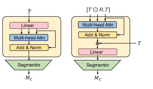
Figure 4: Examples of two Trusty Learner structures. $\oplus$: dimension concatenation.

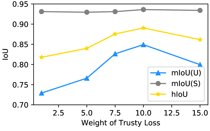
Figure 5: Effect of the weight of trusty loss.

Table 2: Inductive task: Comparison with previous methods.

Methods	PASCAL VOC 2012				COCO-Stuff 164K
	pAcc	mIoU(S)	mIoU(U)	hIoU	pAcc	mIoU(S)	mIoU(U)	hIoU
SPNet [33]	-	78.0	15.6	26.1	-	35.2	8.7	14.0
ZS3 [2]	-	77.3	17.7	28.7	-	34.7	9.5	15.0
GaGNet [14]	80.7	78.4	26.6	39.7	56.6	33.5	12.2	18.2
SIGN [7]	-	75.4	28.9	41.7	-	32.3	15.5	20.9
Joint [1]	-	77.7	32.5	45.9	-	-	-	-
ZegFormer [9]	-	86.4	63.6	73.3	-	36.6	33.2	34.8
zsseg [35]	90.0	83.5	72.5	77.5	60.3	39.3	36.3	37.8
ZegCLIP [40]	94.6	91.9	77.8	84.3	62.0	40.2	41.4	40.8
TagCLIP (Ours)	96.1	93.5	85.2	89.2	63.3	40.7	43.1	41.9

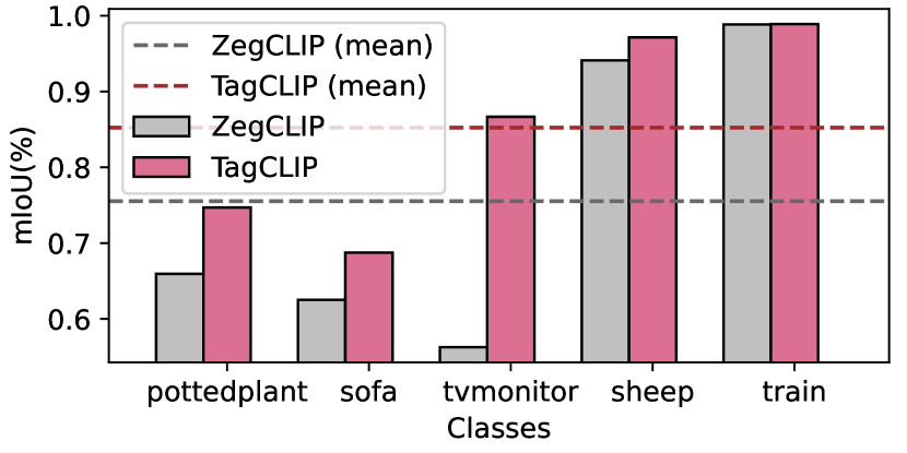
Figure 6: Class-wise performance on unseen classes of PASCAL VOC 2012.

Method	pAcc	mIoU	mAcc
Zegformer [9]	42.3	29.3	56.6
ZegCLIP [40]	60.9	41.2	68.4
TagCLIP (Ours)	63.5	42.6	70.1

Table 3: Generalization performance from COCO-Stuff 164K to PASCAL Context.

Table 4: Transductive task: Comparison with previous methods. ST: Self-Training.

Methods	PASCAL VOC 2012				COCO-Stuff 164K
	pAcc	mIoU(S)	mIoU(U)	hIoU	pAcc	mIoU(S)	mIoU(U)	hIoU
SPNet + ST [33]	-	77.8	25.8	38.8	-	34.6	26.9	30.3
ZS5 [2]	-	78.0	21.2	33.3	-	34.9	10.6	16.2
GaGNet + ST [14]	81.6	78.6	30.3	43.7	56.8	35.6	13.4	19.5
STRICT [24]	-	82.7	35.6	49.8	-	35.3	30.3	34.8
zsseg + ST [35]	88.7	79.2	78.1	79.3	63.8	39.6	43.6	41.5
ZepCLIP + ST [40]	95.1	91.8	82.2	86.7	68.8	40.6	54.8	46.6
DenseCLIP + ST [39]	-	88.8	86.1	87.4	-	38.1	54.7	45.0
ZegCLIP + ST [40]	96.2	92.3	89.9	91.1	69.2	40.6	59.9	48.4
TagCLIP (Ours) + ST	97.2	94.3	92.7	93.5	69.4	40.4	60.0	48.3

Table 5: Supervision task: Comparison with previous methods.

Methods	PASCAL VOC 2012				COCO-Stuff 164K
	pAcc	mIoU(S)	mIoU(U)	hIoU	pAcc	mIoU(S)	mIoU(U)	hIoU
ZegCLIP [40]	96.3	92.4	90.9	91.6	69.9	40.7	63.2	49.6
TagCLIP (Ours)	96.8	93.1	92.8	92.9	69.9	41.3	63.6	50.1

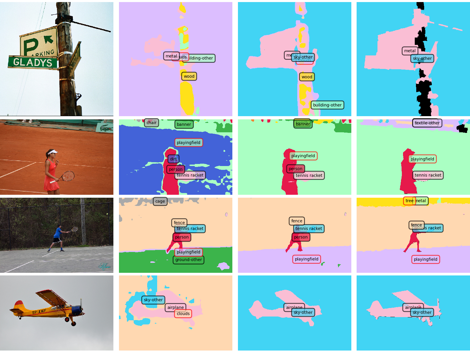
Figure 7: Visualization of segmentation results on COCO-Stuff 164K. Four columns from left to right represent: (a) Original testing images; (b) Results of current SoTA [40]; (c) Results of TagCLIP; (d) Ground truth. The tags with borders in black and red denote seen and unseen classes separately.

4 Experiment

In this section, extensive experiments are conducted to evaluate our proposed TagCLIP.

Datasets.

The experiments are conducted on the following public benchmark datasets: (i) PASCAL VOC 2012 contains 20 classes with 10,582 augmented training and 1,449 testing images. Ignoring the “background” category, we divide the dataset into 15 seen classes and 5 unseen classes. (ii) COCO-Stuff 164K includes 171 categories with 118,287 training and 5,000 testing images. We use 156 and 15 classes as the seen and unseen parts. We also conduct cross-dataset experiments on (iii) PASCAL Context, which contains 60 classes with 4,996 training and 5,104 testing images. We follow the same unseen classes with previous works [9, 14, 35, 39, 40], shown in the Appendix.

Evaluation Metrics.

Following previous works [35, 40], we evaluate pixel-wise classification accuracy (pAcc) and mean of class-wise Intersection over Union (mIoU). We denote mIoU on seen and unseen classes as mIoU(S) and mIoU(U), respectively. We also measure the harmonic mean IoU (hIoU) among seen and unseen classes, which is defined as

$$hIoU=\frac{2\times mIoU(S)\times mIoU(U)}{mIoU(S)+mIoU(U)}$$ (13)

Experimental Setting.

All experiments are based on a pre-trained CLIP ViT-B/16 model. The results of previous works are from [40]. We conduct our experiment on 8 GPUs. The input resolution is set as $512\times 512$ and the batch size is 16. Following previous works [40] for fair comparisons, for inductive zero-shot learning, we train the model with 20K iterations for PASCAL VOC 2012 and 80K for COCO-Stuff 164K. In the transductive setting, we train our proposed model with 10K iterations for PASCAL VOC 2012 and 40K for COCO-Stuff 164K. Then we apply self-training in the rest of the training processes. More details are in the Appendix.

4.1 Ablation Analysis

In this section, we conduct ablation studies to show the effectiveness and respective role of each proposed design.

Ablation of Framework.

Our baseline is the current SoTA one-stage framework [40] of open-vocabulary semantic segmentation, as shown in Tab. 1(a).

Firstly, we directly insert the trusty token into the baseline framework. As shown in Tab. 1(b), the performance on unseen classes falls dramatically due to the poorly-learned token. This gap motivates the design of our Trusty Learner module.

A straightforward way to represent the text-image relation is to concatenate text tokens to the image representation. In our work, we propose two improved variants by respectively concatenating the text tokens $\mathbf{T}$ before and after inputting them into a multi-head attention block. Two examples are shown in Fig. 5. We also experiment with different representations of image features or image-text relation, including patch embeddings $\mathbf{H}$, concatenation $[\mathbf{T},\mathbf{H}]$, similarity matrix $\mathbf{T}\odot\mathbf{H}$, etc. We input them to the Trusty Learner with different $\{\mathbf{Q},\mathbf{K},\mathbf{V}\}$ combinations,

Among the listed experiments, the most impressive performance is achieved by inputting the concatenation ($\mathbf{\hat{T}}$) of the similarity matrix $\mathbf{T}\odot\mathbf{H}$ with text tokens $\mathbf{T}$ into a self-attention block together, as shown in Tab. 1(c). This is understandable because the similarity matrix characterizes the text-image relation and the original text tokens are accessible for the module. With this simple design, the trusty token benefits discrimination and boosts the IoU(U) of the baseline by 7.1%. Furthermore, we weigh the raw segmentation map with the trusty map, which provides an additional 0.3% improvement on novel classes as shown in Tab. 1(d).

Hyper-Parameter $\gamma$.

We follow the weights of losses $\{\alpha,\beta\}=\{20,1\}$ as previous researches [40, 6]. For the weight of our proposed $\mathcal{L}_{A}$ in Sec. 3.3, we conduct experiments in Fig. 5. Results show that $\gamma=10$ reaches the peak of performance, with 93.5% and 85.2% mIoU on seen and unseen classes on PASCAL VOC 2012. Thus, we set $\gamma=10$ in our experimental setting.

4.2 Results

In this section, we compare our proposed TagCLIP with previous approaches.

Inductive Task.

First, we evaluate our method for the inductive open-vocabulary segmentation setting, where both names and images of unseen classes are not accessible during training. Under this setting, our TagCLIP outperforms the mIoU(U) of previous works with significant margins of 7.4% on PASCAL VOC 2012, and of 1.4% on COCO-Stuff 164K. Detailed results are in Tab. 2. The better performance in both unseen and seen classes is consistent with our motivation to improve the model’s discrimination ability.

We illustrate class-wise mIoU in Fig. 6. It shows that TagCLIP beats the current SoTA of every novel category on PASCAL VOC 2012. The margin is especially larger on hard classes, such as the tvmonitor, where TagCLIP outperforms the current SoTA ZegCLIP [40] by 30.4% to 86.7%. The outstanding performance on unseen categories demonstrates the generalization ability of our TagCLIP.

We also illustrate the segmentation visualization results in Fig. 7. Compared with current SoTA, TagCLIP correctly separates the hard unknown classes, like ‘cloud’ with ‘sky-other’, and ‘playingfield’ with ‘dirt’, etc. More visualization results are in the Appendix.

Cross-Dataset Task.

To further explore the cross-domain generalization ability of our approach, we conduct extra experiments in Fig. 6. We train the model on seen classes of COCO-Stuff 164K and evaluate it on PASCAL Context. Outperforming the current SoTA by 1.4%, TagCLIP shows better cross-dataset generalization capability.

Transductive Task.

Besides, we evaluate our method for another setting called transductive zero-shot learning [14, 39]. It allows access to unseen category names during training, but their ground truth masks remained unavailable. TagCLIP is not designed for transductive setting because self-supervision training on accessible unseen names [40, 39, 33] serves the same role. Despite it, TagCLIP still excels the mIoU(U) of current SoTA [40] by 2.8% on PASCAL VOC 2012 and reaches comparative performance on COCO-Stuff 164K. Results are in Tab. 4. It demonstrates TagCLIP’s superior generalization ability to different tasks.

Fully Supervised Task.

We also provide the results trained with full labels in Tab. 5. It demonstrates that TagCLIP improves the upper bound of open-vocabulary segmentation results by 1.9% on PASCAL VOC 2012 and by 0.4% on COCO-Stuff 164K.

5 Conclusion

In this work, we aim to boost open-vocabulary semantic segmentation, particularly toward the long-standing issue of recognizing unseen classes. We propose a novel framework that disentangles the ill-posed baseline into two parallel processes: one performs semantic matching individually, and the other learns to discriminate prediction reliability. Motivated by sentence-level embedding tokens in language modeling, we design a trusty token that captures the known and novel category prediction tendency. With almost no extra overhead from the disentangled objectives, we upgrade the pixel-level generalization capacity of existing models effectively. Our TagCLIP (CLIP adapting with Trusty-guidance) boosts the IoU of unseen classes by 7.4% and 1.7% on PASCAL VOC 2012 and COCO-Stuff 164K.

References

- [1] Donghyeon Baek, Youngmin Oh, and Bumsub Ham. Exploiting a joint embedding space for generalized zero-shot semantic segmentation. In Proceedings of the IEEE/CVF international conference on computer vision, pages 9536–9545, 2021.
- [2] Maxime Bucher, Tuan-Hung Vu, Matthieu Cord, and Patrick Pérez. Zero-shot semantic segmentation. Advances in Neural Information Processing Systems, 32, 2019.
- [3] Liang-Chieh Chen, George Papandreou, Iasonas Kokkinos, Kevin Murphy, and Alan L Yuille. Semantic image segmentation with deep convolutional nets and fully connected crfs. arXiv preprint arXiv:1412.7062, 2014.
- [4] Liang-Chieh Chen, George Papandreou, Florian Schroff, and Hartwig Adam. Rethinking atrous convolution for semantic image segmentation. arXiv preprint arXiv:1706.05587, 2017.
- [5] Bowen Cheng, Ishan Misra, Alexander G Schwing, Alexander Kirillov, and Rohit Girdhar. Masked-attention mask transformer for universal image segmentation. In Proceedings of the IEEE/CVF Conference on Computer Vision and Pattern Recognition, pages 1290–1299, 2022.
- [6] Bowen Cheng, Alex Schwing, and Alexander Kirillov. Per-pixel classification is not all you need for semantic segmentation. Advances in Neural Information Processing Systems, 34:17864–17875, 2021.
- [7] Jiaxin Cheng, Soumyaroop Nandi, Prem Natarajan, and Wael Abd-Almageed. Sign: Spatial-information incorporated generative network for generalized zero-shot semantic segmentation. In Proceedings of the IEEE/CVF International Conference on Computer Vision, pages 9556–9566, 2021.
- [8] Jacob Devlin, Ming-Wei Chang, Kenton Lee, and Kristina Toutanova. Bert: Pre-training of deep bidirectional transformers for language understanding, 2019.
- [9] Jian Ding, Nan Xue, Gui-Song Xia, and Dengxin Dai. Decoupling zero-shot semantic segmentation. In Proceedings of the IEEE/CVF Conference on Computer Vision and Pattern Recognition, pages 11583–11592, 2022.
- [10] Alexey Dosovitskiy, Lucas Beyer, Alexander Kolesnikov, Dirk Weissenborn, Xiaohua Zhai, Thomas Unterthiner, Mostafa Dehghani, Matthias Minderer, Georg Heigold, Sylvain Gelly, Jakob Uszkoreit, and Neil Houlsby. An image is worth 16x16 words: Transformers for image recognition at scale. CoRR, abs/2010.11929, 2020.
- [11] Yu Du, Fangyun Wei, Zihe Zhang, Miaojing Shi, Yue Gao, and Guoqi Li. Learning to prompt for open-vocabulary object detection with vision-language model. In Proceedings of the IEEE/CVF Conference on Computer Vision and Pattern Recognition, pages 14084–14093, 2022.
- [12] Fangxiaoyu Feng, Yinfei Yang, Daniel Cer, Naveen Arivazhagan, and Wei Wang. Language-agnostic bert sentence embedding. arXiv preprint arXiv:2007.01852, 2020.
- [13] Xiuye Gu, Tsung-Yi Lin, Weicheng Kuo, and Yin Cui. Open-vocabulary object detection via vision and language knowledge distillation. arXiv preprint arXiv:2104.13921, 2021.
- [14] Zhangxuan Gu, Siyuan Zhou, Li Niu, Zihan Zhao, and Liqing Zhang. Context-aware feature generation for zero-shot semantic segmentation. In Proceedings of the 28th ACM International Conference on Multimedia, pages 1921–1929, 2020.
- [15] Chao Jia, Yinfei Yang, Ye Xia, Yi-Ting Chen, Zarana Parekh, Hieu Pham, Quoc Le, Yun-Hsuan Sung, Zhen Li, and Tom Duerig. Scaling up visual and vision-language representation learning with noisy text supervision. In International Conference on Machine Learning, pages 4904–4916. PMLR, 2021.
- [16] Jingjing Jiang, Ziyi Liu, and Nanning Zheng. Finetuning pretrained vision-language models with correlation information bottleneck for robust visual question answering. arXiv preprint arXiv:2209.06954, 2022.
- [17] Jingyao Li, Pengguang Chen, Shaozuo Yu, Zexin He, Shu Liu, and Jiaya Jia. Rethinking out-of-distribution (ood) detection: Masked image modeling is all you need. arXiv preprint arXiv:2302.02615, 2023.
- [18] Liunian Harold Li, Mark Yatskar, Da Yin, Cho-Jui Hsieh, and Kai-Wei Chang. Visualbert: A simple and performant baseline for vision and language. arXiv preprint arXiv:1908.03557, 2019.
- [19] Feng Liang, Bichen Wu, Xiaoliang Dai, Kunpeng Li, Yinan Zhao, Hang Zhang, Peizhao Zhang, Peter Vajda, and Diana Marculescu. Open-vocabulary semantic segmentation with mask-adapted clip. arXiv preprint arXiv:2210.04150, 2022.
- [20] Tsung-Yi Lin, Priya Goyal, Ross Girshick, Kaiming He, and Piotr Dollár. Focal loss for dense object detection. In Proceedings of the IEEE international conference on computer vision, pages 2980–2988, 2017.
- [21] Zheyuan Liu, Cristian Rodriguez-Opazo, Damien Teney, and Stephen Gould. Image retrieval on real-life images with pre-trained vision-and-language models. In Proceedings of the IEEE/CVF International Conference on Computer Vision, pages 2125–2134, 2021.
- [22] Jonathan Long, Evan Shelhamer, and Trevor Darrell. Fully convolutional networks for semantic segmentation. In Proceedings of the IEEE conference on computer vision and pattern recognition, pages 3431–3440, 2015.
- [23] Fausto Milletari, Nassir Navab, and Seyed-Ahmad Ahmadi. V-net: Fully convolutional neural networks for volumetric medical image segmentation. In 2016 fourth international conference on 3D vision (3DV), pages 565–571. Ieee, 2016.
- [24] Giuseppe Pastore, Fabio Cermelli, Yongqin Xian, Massimiliano Mancini, Zeynep Akata, and Barbara Caputo. A closer look at self-training for zero-label semantic segmentation. In Proceedings of the IEEE/CVF Conference on Computer Vision and Pattern Recognition, pages 2693–2702, 2021.
- [25] Hieu Pham, Zihang Dai, Golnaz Ghiasi, Kenji Kawaguchi, Hanxiao Liu, Adams Wei Yu, Jiahui Yu, Yi-Ting Chen, Minh-Thang Luong, Yonghui Wu, et al. Combined scaling for open-vocabulary image classification. arXiv e-prints, pages arXiv–2111, 2021.
- [26] Alec Radford, Jong Wook Kim, Chris Hallacy, Aditya Ramesh, Gabriel Goh, Sandhini Agarwal, Girish Sastry, Amanda Askell, Pamela Mishkin, Jack Clark, et al. Learning transferable visual models from natural language supervision. In International conference on machine learning, pages 8748–8763. PMLR, 2021.
- [27] Olaf Ronneberger, Philipp Fischer, and Thomas Brox. U-net: Convolutional networks for biomedical image segmentation. In Medical Image Computing and Computer-Assisted Intervention–MICCAI 2015: 18th International Conference, Munich, Germany, October 5-9, 2015, Proceedings, Part III 18, pages 234–241. Springer, 2015.
- [28] Karen Simonyan and Andrew Zisserman. Very deep convolutional networks for large-scale image recognition. arXiv preprint arXiv:1409.1556, 2014.
- [29] Robin Strudel, Ricardo Garcia, Ivan Laptev, and Cordelia Schmid. Segmenter: Transformer for semantic segmentation. In Proceedings of the IEEE/CVF international conference on computer vision, pages 7262–7272, 2021.
- [30] Weijie Su, Xizhou Zhu, Yue Cao, Bin Li, Lewei Lu, Furu Wei, and Jifeng Dai. Vl-bert: Pre-training of generic visual-linguistic representations. arXiv preprint arXiv:1908.08530, 2019.
- [31] Keigo Takahashi and Danushka Bollegala. Unsupervised attention-based sentence-level meta-embeddings from contextualised language models. arXiv preprint arXiv:2204.07746, 2022.
- [32] Zhaoqing Wang, Yu Lu, Qiang Li, Xunqiang Tao, Yandong Guo, Mingming Gong, and Tongliang Liu. Cris: Clip-driven referring image segmentation. In Proceedings of the IEEE/CVF conference on computer vision and pattern recognition, pages 11686–11695, 2022.
- [33] Yongqin Xian, Subhabrata Choudhury, Yang He, Bernt Schiele, and Zeynep Akata. Semantic projection network for zero-and few-label semantic segmentation. In Proceedings of the IEEE/CVF Conference on Computer Vision and Pattern Recognition, pages 8256–8265, 2019.
- [34] Enze Xie, Wenhai Wang, Zhiding Yu, Anima Anandkumar, Jose M Alvarez, and Ping Luo. Segformer: Simple and efficient design for semantic segmentation with transformers. Advances in Neural Information Processing Systems, 34:12077–12090, 2021.
- [35] Mengde Xu, Zheng Zhang, Fangyun Wei, Yutong Lin, Yue Cao, Han Hu, and Xiang Bai. A simple baseline for zero-shot semantic segmentation with pre-trained vision-language model. arXiv preprint arXiv:2112.14757, 2021.
- [36] Bowen Zhang, Zhi Tian, Quan Tang, Xiangxiang Chu, Xiaolin Wei, Chunhua Shen, et al. Segvit: Semantic segmentation with plain vision transformers. Advances in Neural Information Processing Systems, 35:4971–4982, 2022.
- [37] Hang Zhang, Kristin Dana, Jianping Shi, Zhongyue Zhang, Xiaogang Wang, Ambrish Tyagi, and Amit Agrawal. Context encoding for semantic segmentation. In Proceedings of the IEEE conference on Computer Vision and Pattern Recognition, pages 7151–7160, 2018.
- [38] Sixiao Zheng, Jiachen Lu, Hengshuang Zhao, Xiatian Zhu, Zekun Luo, Yabiao Wang, Yanwei Fu, Jianfeng Feng, Tao Xiang, Philip HS Torr, et al. Rethinking semantic segmentation from a sequence-to-sequence perspective with transformers. In Proceedings of the IEEE/CVF conference on computer vision and pattern recognition, pages 6881–6890, 2021.
- [39] Chong Zhou, Chen Change Loy, and Bo Dai. Denseclip: Extract free dense labels from clip. arXiv preprint arXiv:2112.01071, 2021.
- [40] Ziqin Zhou, Bowen Zhang, Yinjie Lei, Lingqiao Liu, and Yifan Liu. Zegclip: Towards adapting clip for zero-shot semantic segmentation. arXiv preprint arXiv:2212.03588, 2022.