Tests for ultrahigh-dimensional partially linear regression models

Abstract

In this paper, we consider tests for ultrahigh-dimensional partially linear regression models. The presence of ultrahigh-dimensional nuisance covariates and unknown nuisance function makes the inference problem very challenging. We adopt machine learning methods to estimate the unknown nuisance function and introduce quadratic-form test statistics. Interestingly, though the machine learning methods can be very complex, under suitable conditions, we establish the asymptotic normality of our introduced test statistics under the null hypothesis and local alternative hypotheses. We further propose a power-enhanced procedure to improve the test statistics’ performance. Two thresholding determination methods are provided for the power-enhanced procedure. We show that the power-enhanced procedure is powerful to detect signals under either sparse or dense alternatives and it can still control the type-I error asymptotically under the null hypothesis. Numerical studies are carried out to illustrate the empirical performance of our introduced procedures.

Keywords: Machine learning; Partially linear model; Power enhancement; Significance testing; Ultrahigh dimensionality.

1 Introduction

Let $Y\in\mathbb{R}$ be the response along with covariates $\mathbf{X}=(X_{1},\ldots,X_{p_{1}})^{\top}\in\mathbb{R}^{p_{1}}$ and $\mathbf{Z}=(Z_{1},\ldots,Z_{p_{2}})^{\top}\in\mathbb{R}^{p_{2}}$. We consider the following ultrahigh-dimensional partially linear model,

$$Y=\mathbf{X}^{\top}\bm{\beta}+g(\mathbf{Z})+\epsilon\quad\mathrm{with}\quad\epsilon\bot\!\!\!\bot\mathbf{X}.$$ (1.1)

Here $\bm{\beta}\in\mathbb{R}^{p_{1}}$ is an unknown regression coefficient, $g(\cdot):\mathbb{R}^{p_{2}}\rightarrow\mathbb{R}$ is an unknown smooth function, and $\epsilon$ is a random error term with $\mathbb{E}(\epsilon)=0$ and $\mbox{Var}(\epsilon)=\sigma^{2}$. Due to its flexibility and interpretability, the partially linear model (Härdle et al.,, 2000) is widely used. In this paper, we aim to test whether the covariates of primary interest $\mathbf{X}$ contribute to the response $Y$ given the other nuisance covariates $\mathbf{Z}$. Under the above model (1.1), this problem can be formulated as the following hypothesis testing problem,

$$\mathbb{H}_{0}:\bm{\beta}=\bm{0},\qquad\mathrm{versus}\qquad\mathbb{H}_{1}:\bm{\beta}\neq\bm{0}.$$ (1.2)

The above testing problem is of great importance in practice. For instance, in association analysis, researchers usually test the significance of a gene pathway consisting of ultrahigh-dimensional genes for the same biological function, given the other ultrahigh-dimensional genes. To address these kinds of problems, in this paper, we allow both the covariates of primary interest $\mathbf{X}$ and the nuisance covariates $\mathbf{Z}$ to be ultrahigh-dimensional, that is, $p_{1}$ and $p_{2}$ both can be exponential order of the sample size.

Under the high-dimensional linear or generalized linear models, many authors considered the above testing problem. Actually, Zhang and Cheng, (2017) and Dezeure et al., (2017) introduced coordinate-based maximum tests. They first obtained debiased/desparsified Lasso estimators (Zhang and Zhang,, 2014; Van de Geer et al.,, 2014; Javanmard and Montanari,, 2014) for each component and then used the maximum of these estimators as test statistics. This idea was also considered by many other authors. See for instance Ning and Liu, (2017) and Ma et al., (2021). These maximum-type methods are computationally expensive and generally are not powerful in the presence of dense alternatives. When the alternatives are really dense, which means the parametric vector contains many non-zero small regression coefficients, the quadratic-form test procedure introduced by Zhong and Chen, (2011) is a powerful approach. The procedures in Zhong and Chen, (2011) are further extended by Guo and Chen, (2016) to the generalized linear model. However, the procedures in Zhong and Chen, (2011) and Guo and Chen, (2016) can not deal with ultrahigh-dimensional nuisance covariates. To solve this critical issue, Chen et al., (2023) introduced penalized estimators to the original procedure in Guo and Chen, (2016). Theoretically, the dimension of the parametric vector of interest can only grow polynomially with the sample size to guarantee nontrivial power. Yang et al., (2022) made a deep theoretical investigation of the test procedure in Chen et al., (2023). They developed new techniques and obtained the limiting distributions under the null and local alternative hypotheses. Their results allow both $\mathbf{X}$ and $\mathbf{Z}$ to be ultrahigh-dimensional. However, all these papers focus on high-dimensional parametric models and can not be directly extended to the above partially linear model (1.1).

There are also some studies about (1.2) under the partially linear model. See for instance Wang and Cui, (2017, 2020), Liu et al., (2020) and Zhao et al., (2023). However, these studies only focus on low-dimensional nuisance covariates. The low-dimension nature of the nuisance covariates $\mathbf{Z}$ in these papers enables the authors to estimate the unknown smooth function $g(\mathbf{Z})$ using classical nonparametric methods, such as the kernel method. However, it is widely recognized that the kernel method can fail when the dimension of $\mathbf{Z}$ is relatively high. Thus these procedures can not handle the testing problem (1.2) when both the covariates of interest and the nuisance covariates are ultrahigh-dimensional.

The existing works motivate the investigation of the current paper. Different from existing papers, we allow the covariates of primary interest and the nuisance covariates to be ultrahigh-dimensional and also allow the smooth function $g(\cdot)$ to be unknown. To estimate the smooth function $g(\cdot)$ efficiently, some flexible machine learning (ML) methods are adopted. However, a direct application would make the theoretical analysis very difficult due to the complex and even black-box nature of ML methods. To this end, sample-splitting is adopted. Actually, we first randomly split the data into two parts. We use one part to estimate the smooth function $g(\cdot)$ by some ML methods. We then use the other part to construct quadratic-form test statistics. Under mild conditions, we obtain the limiting distributions of the constructed test statistics under the null and local alternative hypotheses even though we estimate the smooth function $g(\cdot)$ by some black-box ML methods.

In this paper, we further propose power-enhanced test procedures to achieve good power performance under general alternatives. Actually, when the parametric vector of interest is extremely sparse, which means only a very small subset of covariates contribute to the response, the power of quadratic-form test statistics can be low (Xu et al.,, 2016; Chen et al.,, 2019; Yu et al.,, 2022). Although the coordinate-based maximum tests are powerful in detecting sparse alternatives, they perform poorly when the parametric vector of interest is dense. In practice, the sparsity of the parametric vector is typically unknown, making it challenging to choose a powerful test. To overcome this issue, we are inspired by the original paper of Fan et al., (2015) and introduce power-enhanced test statistics. Fan et al., (2015) considered a quadratic-form OLS-based statistic with asymptotically normal marginal distributions. However, in contrast to Fan et al., (2015), the distributions of our marginal test statistics being degenerate $U$-statistics are no longer asymptotically normal under the null hypothesis. We need to construct power-enhanced test statistics based on degenerate $U$-statistics. For the power-enhanced procedures, one hard thresholding level and one soft thresholding level are given by investigating the tail probabilities of our marginal test statistics. We demonstrate that the enhanced test has no size distortion asymptotically, and the power is indeed enhanced under more general alternatives.

The remainder of the paper is organized as follows. In Section 2, we introduce our testing procedures and derive their limiting distributions. In Section 3, we propose power-enhanced tests and investigate their theoretical properties. Section 4 presents simulation studies. Real data example is analyzed in Section 5. Section 6 offers some discussions and conclusions. All the technical proofs and additional simulation results are relegated to the Supplementary Material.

Notations. The following notation is adopted throughout this paper. For a $d$-dimensional vector $\mathbf{U}=(U_{1},\ldots,U_{d})^{\top}\in\mathbb{R}^{d}$, we define $\|\mathbf{U}\|_{l}=(\sum_{j=1}^{d}|U_{j}|^{l})^{1/l}$ with $1\leq l<\infty$ and $\|\mathbf{U}\|_{\infty}=\max_{1\leq j\leq d}|U_{j}|$ to denote $L_{q}$ and $L_{\infty}$ norms of $\mathbf{U}$. A random variable $X$ is sub-Gaussian if the moment generating function (MGF) of $X^{2}$ is bounded at some point, namely $\mathbb{E}\exp(X^{2}/K^{2})\leq 2$, where $K$ is a positive constant. A random variable $Y$ is $\operatorname{\mathit{sub-Exponential}}$ if the MGF of $\lvert Y\rvert$ is bounded at some point, namely $\mathbb{E}\exp(\lvert Y\rvert/K^{\prime})\leq 2$, where $K^{\prime}$ is a positive constant. The sub-Gaussian norm of a sub-Gaussian random variable $X$ is defined as $\|X\|_{\psi_{2}}=\inf\{t>0:\mathbb{E}\exp(X^{2}/t^{2})\leq 2\}$. For $q_{1}\times q_{2}$-dimensional matrix $\mathbf{A}$, we define $\|\mathbf{A}\|_{\infty}=\max_{ij}|A_{ij}|$, where $A_{ij}$ is the $(i,j)$-th element of $\mathbf{A}$. For notational simplicity, we let $c$ and $C$ be generic constants.

2 Quadratic-form test statistics and their properties

Suppose that $\mathcal{D}=(\mathbf{X}_{i},\mathbf{Z}_{i},Y_{i})_{i=1}^{N}$ with $N=2n$ is an independent and identically distributed random sample from the population $(\mathbf{X},\mathbf{Z},Y)$. Denote $S(\mathbf{Z})=\{Y-g(\mathbf{Z})\}\mathbf{X}$. Under the null hypothesis, $\mathbb{E}[S(\mathbf{Z})]^{\top}\mathbb{E}[S(\mathbf{Z})]=0$, while under the alternative hypothesis, $\mathbb{E}[S(\mathbf{Z})]^{\top}\mathbb{E}[S(\mathbf{Z})]>0$. This then implies that we can construct test statistics based on sample versions of $\mathbb{E}[S(\mathbf{Z})]^{\top}\mathbb{E}[S(\mathbf{Z})]$. Inspired by Zhong and Chen, (2011), Guo and Chen, (2016), Chen et al., (2023) and Yang et al., (2022), we may consider the following quadratic-form test statistic,

$$T_{N}=\frac{1}{N}\sum_{i\neq j}\{Y_{i}-\widehat{g}(\mathbf{Z}_{i})\}\{Y_{j}-\widehat{g}(\mathbf{Z}_{j})\}\mathbf{X}_{i}^{\top}\mathbf{X}_{j}.$$ (2.1)

Here $\widehat{g}(\cdot)$ is a suitable estimator of $g(\cdot)$ obtained from $(\mathbf{Z}_{i},Y_{i})_{i=1}^{N}$. The advantage of not using $\mathbf{X}_{i},i=1,\cdots,N$ for estimation is that we can sufficiently exploit the model structure under the null hypothesis and avoid imposing strong assumptions on the dimension and sparsity of $\bm{\beta}$.

Since the dimension of $\mathbf{Z}$ is very high, classical nonparametric methods such as the kernel method fail. To handle this issue, we use some flexible machine learning (ML) methods such as Lasso, Random Forest, and Neural Nets to obtain the estimator $\widehat{g}(\cdot)$. However, a direct involvement of $\widehat{g}(\cdot)$ in the above $T_{N}$ makes it very difficult to analyze the properties of the test statistic $T_{N}$ due to the possible over-fitting/high-complexity phenomena that commonly occur in ML estimates. To this end, the sample-splitting idea is adopted to separate the estimation of the nuisance function from the construction of test statistics. The sample-splitting idea is a powerful approach that has been employed by many authors in different problems. See for instance Fan et al., (2012), Chernozhukov et al., (2018), Du et al., (2021) and Cai et al., (2023).

To be precise, we first randomly split data $\mathcal{D}$ into two parts: $\mathcal{D}_{1}$ and $\mathcal{D}_{2}$ with equal size, $|\mathcal{D}_{k}|=n,k=1,2$. We estimate $g(\cdot)$ by some ML algorithms based on the data $\mathcal{D}_{k}$ and denote the estimator as $\widehat{g}_{k}(\cdot)$. We then construct test statistics based on the other part $\mathcal{D}_{3-k}$. That is, we consider the following test statistics,

$$T_{nk}=\frac{1}{n}\sum_{i\neq j,i,j\in\mathcal{D}_{3-k}}\{Y_{i}-\widehat{g}_{k}(\mathbf{Z}_{i})\}\{Y_{j}-\widehat{g}_{k}(\mathbf{Z}_{j})\}\mathbf{X}_{i}^{\top}\mathbf{X}_{j},\quad k=1,2.$$ (2.2)

The above test statistics $T_{nk}$ are also inspired by the elegant double machine learning framework in Chernozhukov et al., (2018). In Chernozhukov et al., (2018), the dimension of interested covariates $\mathbf{X}$ is fixed. While here we focus on the situation that $\mathbf{X}$ is ultrahigh-dimensional. One may extend the approach of Chernozhukov et al., (2018) by adopting the coordinate-based maximum tests. That is, for each element of $\mathbf{X}$, use the double machine learning approach to construct element-wise test statistics and then consider the maximum of these element-wise test statistics. Compared with coordinate-based maximum tests, here we only need to estimate $g(\cdot)$ twice, and thus the computational cost is significantly reduced. Further as discussed in the Introduction, coordinate-based maximum tests are not powerful for dense alternatives.

In the following, we will show that the above constructed test statistics $T_{nk}$ are asymptotically normal under the null hypothesis even if we estimate the smooth function $g(\cdot)$ by black-box ML techniques.

2.1 Asymptotic null distribution

Let $\mathbf{V}=(\mathbf{X}^{\top},\mathbf{Z}^{\top})^{\top}$, $\bm{\Sigma}_{\mathbf{X}}=\mathbb{E}(\mathbf{X}\mathbf{X}^{\top})$, $\bm{\Sigma}_{\mathbf{X}\mathbf{Z}}=\mathbb{E}(\mathbf{X}\mathbf{Z}^{\top})$, $\bm{\Sigma}_{\mathbf{Z}\mathbf{X}}=\mathbb{E}(\mathbf{Z}\mathbf{X}^{\top})$ and $p=p_{1}+p_{2}$. Denote $\bm{\mu}_{gk}=\mathbb{E}[\{g(\mathbf{Z})-\widehat{g}_{k}(\mathbf{Z})\}\mathbf{X}]$ and $\Lambda_{\mathbf{X}}=2\sigma^{4}\mathrm{tr}(\bm{\Sigma}_{\mathbf{X}}^{2})$. We impose the following technical assumptions to study the asymptotic null distributions of the test statistics $T_{nk}\ (k=1,2)$.

Assumption 2.1.

Assume that $\mathrm{tr}(\bm{\Sigma}^{4}_{\mathbf{X}})=o(\mathrm{tr}^{2}(\bm{\Sigma}_{\mathbf{X}}^{2}))$ and $\mathrm{tr}(\bm{\Sigma}_{\mathbf{X}}^{2})\rightarrow\infty$ as $(n,p_{1})\rightarrow\infty$.

Assumption 2.2.

Let $\mathbf{A}_{1}$ and $\mathbf{A}_{2}$ be two $p_{1}\times p_{1}$ semi-positive matrices. Assume that $\mathbb{E}\biggl{(}\prod_{i=1}^{2}\mathbf{X}^{\top}\mathbf{A}_{i}\mathbf{X}\biggr{)}\leq C\prod_{i=1}^{2}\mathrm{tr}(\mathbf{A}_{i}\bm{\Sigma}_{\mathbf{X}})$.

Assumption 2.3.

Assume that $n\bm{\mu}_{gk}^{\top}\bm{\mu}_{gk}=o(\sqrt{\Lambda_{\mathbf{X}}})$.

Assumption 2.4.

Assume that $c<\mathbb{E}(\epsilon^{2})$ and $\mathbb{E}(\epsilon^{4})<C$ for some positive constants $c,C$.

Assumption 2.5.

Assume that $\mathbb{E}[\{g(\mathbf{Z})-\widehat{g}_{k}(\mathbf{Z})\}^{4}]=o(1)$.

Assumption 2.1 is a mild condition that is commonly imposed in the literature (Zhong and Chen,, 2011; Guo and Chen,, 2016; Cui et al.,, 2018). Note that if all the eigenvalues of $\bm{\Sigma}_{\mathbf{X}}$ are bounded, then $\mathrm{tr}(\bm{\Sigma}^{4}_{\mathbf{X}})=o(\mathrm{tr}^{2}(\bm{\Sigma}_{\mathbf{X}}^{2}))$ holds trivially. In Assumption 2.2, we only make a very mild moment condition and make no distribution assumption on $\mathbf{X}$ nor $\mathbf{Z}$. Note that this assumption is weaker than the pseudo-independence assumption and the elliptical distribution assumption, which are commonly assumed in the literature (Zhong and Chen,, 2011; Guo and Chen,, 2016; Cui et al.,, 2018). Assumption 2.3 is imposed to control the impact of the bias from $\widehat{g}_{k}(\mathbf{Z})$ on the asymptotic distributions of $T_{nk}$. In the following Remark 2.1, we make further discussions about this assumption. In Assumption 2.4, mild moment conditions for the error term are imposed. Assumption 2.5 is a mild condition on the rate of estimating the nuisance function $g(\cdot)$, which is available for many ML methods. In the above assumptions, the covariates of primary interest $\mathbf{X}$ and the nuisance covariates $\mathbf{Z}$ are both allowed to be ultrahigh-dimensional.

Remark 2.1.

Suppose that the model (1.1) is linear with $g(\mathbf{Z})=\mathbf{Z}^{\top}\bm{\gamma}$, where $\bm{\gamma}$ is a $p_{2}$-dimensional regression coefficient. Further let $\widehat{\bm{\gamma}}_{k}$ be a penalized estimator of $\bm{\gamma}$. By Hölder’s inequality, we have

$$n\bm{\mu}_{gk}^{\top}\bm{\mu}_{gk}=n(\bm{\gamma}-\widehat{\bm{\gamma}}_{k})^{\top}\mathbb{E}(\mathbf{Z}\mathbf{X}^{\top})\mathbb{E}(\mathbf{X}\mathbf{Z}^{\top})(\bm{\gamma}-\widehat{\bm{\gamma}}_{k})\leq n\|\bm{\gamma}-\widehat{\bm{\gamma}}_{k}\|_{1}^{2}\|\bm{\Sigma}_{\mathbf{Z}\mathbf{X}}\bm{\Sigma}_{\mathbf{X}\mathbf{Z}}\|_{\infty}.$$

Note that

$$(\bm{\Sigma}_{\mathbf{Z}\mathbf{X}}\bm{\Sigma}_{\mathbf{X}\mathbf{Z}})_{ij}=\sum_{l}\mathbb{E}(Z_{i}X_{l})\mathbb{E}(X_{l}Z_{j})\leq\frac{1}{2}\sum_{l}\mathbb{E}^{2}(Z_{i}X_{l})+\mathbb{E}^{2}(X_{l}Z_{j})\leq\varrho^{2}.$$

Here $\varrho^{2}=\max_{1\leq h\leq p_{2}}\|\mathbb{E}(Z_{h}\mathbf{X})\|_{2}^{2}$. Generally, it holds that $\|\bm{\gamma}-\widehat{\bm{\gamma}}_{k}\|_{1}=O_{p}(s_{2}\sqrt{\log p_{2}/n})$, where $s_{2}$ is the sparsity level of $\bm{\gamma}$. Many penalized estimators, such as Lasso, SCAD and MCP, can achieve this $L_{1}$ error bound of $\widehat{\bm{\gamma}}_{k}$. See for instance Fan et al., (2020). A sufficient condition for Assumption 2.3 thereby is $s_{2}^{2}\log p_{2}\varrho^{2}=o(\sqrt{\Lambda_{\mathbf{X}}})$. When the eigenvalues of the variance matrix of $\mathbf{V}$ are all bounded, $\varrho^{2}$ is bounded and $\Lambda_{\mathbf{X}}$ is in the order of $p_{1}$. Then the condition $s_{2}^{2}\log p_{2}\varrho^{2}=o(\sqrt{\Lambda_{\mathbf{X}}})$ can be simplified as $s^{2}_{2}\log p_{2}=o(\sqrt{p_{1}}).$ When $p_{1}\geq cn^{2}$, this condition is then even weaker than $s_{2}^{2}\log p_{2}=o(n)$. In other words, Assumption 2.3 holds when the covariates $\mathbf{X}$ and $\mathbf{Z}$ are both ultrahigh-dimensional, reaching the exponential order of the sample size.

Theorem 2.1.

Under $\mathbb{H}_{0}$, if Assumptions 2.1-2.5 hold, we have

$$\frac{T_{nk}}{\sqrt{\Lambda_{\mathbf{X}}}}\stackrel{{\scriptstyle d}}{{\rightarrow}}N(0,1)\quad\text{as}\ (n,p_{1},p_{2})\rightarrow\infty,$$ (2.3)

where $T_{nk}$ is defined in (2.2) and $\Lambda_{\mathbf{X}}=2\sigma^{4}\mathrm{tr}(\bm{\Sigma}_{\mathbf{X}}^{2})$.

In the above Theorem, we establish the limiting null distribution of the proposed test statistics $T_{nk}\ (k=1,2)$. Notably, our test statistics allow very flexible and complex ML methods.

For inference, we need an estimate of $\Lambda_{\mathbf{X}}$ involved in Theorem 2.1. We define

$$\widehat{\Lambda}_{\mathbf{X},k}=2\widehat{\sigma}_{k}^{4}\widehat{\mathrm{tr}(\bm{\Sigma}_{\mathbf{X}}^{2})}_{k}.$$ (2.4)

Here we use the ratio consistent estimator of $\mathrm{tr}(\bm{\Sigma}^{2}_{\mathbf{X}})$ following Zhong and Chen, (2011), that is

$$\widehat{\mathrm{tr}(\bm{\Sigma}^{2}_{\mathbf{X}})}_{k}=\frac{1}{2\binom{n}{4}}\sum_{i_{1}<i_{2}<i_{3}<i_{4}\in\mathcal{D}_{3-k}}(\mathbf{X}_{i_{1}}-\mathbf{X}_{i_{2}})^{\top}(\mathbf{X}_{i_{3}}-\mathbf{X}_{i_{4}})(\mathbf{X}_{i_{2}}-\mathbf{X}_{i_{3}})^{\top}(\mathbf{X}_{i_{4}}-\mathbf{X}_{i_{1}}).$$

While for the variance $\sigma^{2}$, we can estimate it as follows,

$$\widehat{\sigma}^{2}_{k}=\frac{1}{n}\sum_{i\in\mathcal{D}_{3-k}}\{Y_{i}-\widehat{g}_{k}(\mathbf{Z}_{i})\}^{2}.$$

Next we obtain the normalized test statistics $\widetilde{T}_{nk}\ (k=1,2)$ by plugging the estimator of $\Lambda_{\mathbf{X}}$ into (2.3). From Theorem 2.1 and the Slutsky Theorem, we further conclude that

$$\widetilde{T}_{nk}=\frac{T_{nk}}{\sqrt{\widehat{\Lambda}_{\mathbf{X},k}}}\stackrel{{\scriptstyle d}}{{\rightarrow}}N(0,1)\quad\text{as}\ (n,p_{1},p_{2})\rightarrow\infty.$$ (2.5)

It is noteworthy that the data-splitting statistics given above have the drawback that only the information from half of the data is exploited to make inference, which can lead to a significant power loss. To deal with this issue, we can utilize cross-fitting to achieve further improvement. See for instance Fan et al., (2012), Chernozhukov et al., (2018) and Cai et al., (2023). As above, we can construct two test statistics $\widetilde{T}_{n1}$ and $\widetilde{T}_{n2}$. Further note that they are asymptotically independent. From Theorem 2.1 and by averaging the two resulting statistics, we have the following limiting distribution,

$$\widetilde{T}_{n}=\frac{1}{\sqrt{2}}(\widetilde{T}_{n1}+\widetilde{T}_{n2})\stackrel{{\scriptstyle d}}{{\rightarrow}}N(0,1),\quad\text{as}\ (n,p_{1},p_{2})\rightarrow\infty.$$ (2.6)

Hence an asymptotic $\alpha$-level test rejects $\mathbb{H}_{0}$ if

$$\widetilde{T}_{n}\geq z_{\alpha}.$$

Here $z_{\alpha}$ is the upper-$\alpha$ quantile of the standard normal distribution, and $\alpha$ is the significance level. For the sake of clarity, the detailed algorithm for making inference on $\bm{\beta}$ is provided in Algorithm 1.

Algorithm 1 Inference procedure for $\mathbb{H}_{0}$

0:  Data $\mathcal{D}=(\mathbf{X}_{i},\mathbf{Z}_{i},Y_{i})_{i=1}^{N}$ with $N=2n$.

0:  $p$-value for $\mathbb{H}_{0}:\bm{\beta}=\bm{0}$.

  Step 1. Randomly split the data $\mathcal{D}$ into two parts $\mathcal{D}_{1}$ and $\mathcal{D}_{2}$ with equal sample size $n$.

  Step 2. Estimate the nuisance function $g(\cdot)$ by some ML algorithms on the data $\mathcal{D}_{k}$, and denote the estimator as $\widehat{g}_{k}(\cdot)$.

  Step 3. Construct the test statistic $T_{nk}$ as shown in (2.2) based on the data $\mathcal{D}_{3-k}$. Calculate the test statistic $\widetilde{T}_{nk}$ using the formulas (2.4) and (2.5).

  Step 4. Let $k=1,2$ and repeat Step 2 and Step 3 to obtain the test statistics $\widetilde{T}_{n1}$ and $\widetilde{T}_{n2}$. Further calculate $\widetilde{T}_{n}=(\widetilde{T}_{n1}+\widetilde{T}_{n2})/\sqrt{2}$.

  Step 5. Calculate the $p$-value by $1-\Phi(\widetilde{T}_{n})$, where $\Phi(\cdot)$ is the cumulative distribution function of the standard normal distribution. The null hypothesis $\mathbb{H}_{0}$ is rejected if $1-\Phi(\widetilde{T}_{n})\leq\alpha$.

To reduce the randomness induced by data splitting, we further consider an ensemble testing procedure based on multiple data splitting. This is an adoption of the procedure in Meinshausen et al., (2009). The detailed algorithm is presented in the Supplementary Material. With this ensemble testing procedure, the type-I error can still be asymptotically controlled.

2.2 Power analysis

In this subsection, we present power analysis for the proposed test statistics. Consider the following family of local alternatives,

$$\mathscr{L}(\bm{\beta})=\left\{\bm{\beta}\in\mathbb{R}^{p_{1}}\bigg{|}\bm{\beta}^{\top}\bm{\Sigma}_{\mathbf{X}}\bm{\beta}=o(1),\ \bm{\beta}^{\top}\bm{\Sigma}_{\mathbf{X}}^{2}\bm{\beta}=o\left(\frac{\Lambda_{\mathbf{X}}}{n^{2}\bm{\mu}_{gk}^{\top}\bm{\mu}_{gk}}\right)\ \text{and}\ \bm{\beta}^{\top}\bm{\Sigma}_{\mathbf{X}}^{3}\bm{\beta}=o\left(\frac{\Lambda_{\mathbf{X}}}{n}\right)\right\}.$$

The following theorem gives the asymptotic behaviour of the proposed test statistics $T_{nk}\ (k=1,2)$ under the above local alternative hypotheses.

Theorem 2.2.

Under conditions in Theorem 2.1, and for $\bm{\beta}\in\mathscr{L}(\bm{\beta})$, we have

$$\frac{T_{nk}-n\bm{\beta}^{\top}\bm{\Sigma}_{\mathbf{X}}^{2}\bm{\beta}}{\sqrt{\Lambda_{\mathbf{X}}}}\stackrel{{\scriptstyle d}}{{\rightarrow}}N(0,1)\quad\text{as}\ (n,p_{1},p_{2})\rightarrow\infty.$$

Regard $n\bm{\beta}^{\top}\bm{\Sigma}_{\mathbf{X}}^{2}\bm{\beta}$ as the signal strength and the power is largely determined by the following signal-to-noise ratio,

$$\mathrm{SNR}=\frac{n\bm{\beta}^{\top}\bm{\Sigma}_{\mathbf{X}}^{2}\bm{\beta}}{\sqrt{\Lambda_{\mathbf{X}}}}.$$

Thus when the signal-to-noise ratio is large, our proposed test statistics can have large powers for the alternative hypotheses $\mathscr{L}(\bm{\beta})$.

In above theorems, we assume $n\bm{\mu}_{gk}^{\top}\bm{\mu}_{gk}=o(\sqrt{\Lambda_{\mathbf{X}}})$ in Assumption 2.3. However, this assumption may not hold under certain alternative hypotheses. In the following, we investigate the performance of $T_{nk}$ when we can not estimate $g(\cdot)$ very well.

Assumption 2.6.

Assume that $\mathbb{E}[\{g(\mathbf{Z})-\widehat{g}_{k}(\mathbf{Z})\}^{4}]=O(1)$.

In Assumption 2.5, we require that $\mathbb{E}[\{g(\mathbf{Z})-\widehat{g}_{k}(\mathbf{Z})\}^{4}]=o(1)$. But in above Assumption 2.6, we allow $\widehat{g}_{k}(\mathbf{Z})$ estimate $g(\mathbf{Z})$ even inconsistently. Actually since we obtain $\widehat{g}_{k}(\mathbf{Z})$ from $(\mathbf{Z}_{i},Y_{i}),i\in\mathcal{D}_{k}$, $\widehat{g}_{k}(\mathbf{Z})$ aims to estimate $g^{*}(\mathbf{Z})=\mathbb{E}(Y|\mathbf{Z})=g(\mathbf{Z})+\mathbb{E}(\mathbf{X}|\mathbf{Z})^{\top}\bm{\beta}$, which is different from $g(\mathbf{Z})$ under alternative hypothesis.

We consider the following family of alternative hypotheses,

$$\mathscr{L}^{\text{A}}(\bm{\beta})=\left\{\bm{\beta}\in\mathbb{R}^{p_{1}}\Big{|}\sqrt{\Lambda_{\mathbf{X}}}=o\big{(}n\|\bm{\Sigma}_{\mathbf{X}}\bm{\beta}+\bm{\mu}_{gk}\|_{2}^{2}\big{)},\bm{\beta}^{\top}\bm{\Sigma}_{\mathbf{X}}\bm{\beta}=O(1)\right\}.$$

The above alternative hypotheses correspond to the situation that either the signal-to-noise ratio, ${n\bm{\beta}^{\top}\bm{\Sigma}_{\mathbf{X}}^{2}\bm{\beta}}/{\sqrt{\Lambda_{\mathbf{X}}}}$ is very large or the bias term $n\bm{\mu}_{gk}^{\top}\bm{\mu}_{gk}$ from $\widehat{g}_{k}(\cdot)$ relative to $\sqrt{\Lambda_{\mathbf{X}}}$ is large. The following theorem shows that under the above alternatives, the power of our proposed test statistics can be asymptotically 1.

Theorem 2.3.

If Assumptions 2.2, 2.4 and 2.6 hold, and for $\bm{\beta}\in\mathscr{L}^{\text{A}}(\bm{\beta})$, we have

$$\frac{T_{nk}}{\sqrt{\Lambda_{\mathbf{X}}}}{\rightarrow}\infty\quad\text{as}\ (n,p_{1},p_{2})\rightarrow\infty.$$

This theorem implies that even if we can not estimate the function $g(\cdot)$ well under alternative hypotheses, we can still have high detection power. Further note that in the above theorem, Assumption 2.1 is not required. From the theoretical analysis, it is known that Assumption 2.1 is adopted to establish the asymptotic normality of our proposed test statistics by applying the martingale central limit theorems, while in the above theorem, we only need to show that the variance of $T_{nk}$ is dominated by the expectation of $T_{nk}$.

3 Power-enhanced tests

This section discusses power-enhanced tests and presents the theoretical properties of power-enhanced statistics. Two techniques to determine the threshold are also provided.

In Section 2, we establish some promising asymptotic properties for the quadratic-form test statistics $T_{nk}$, such quadratic-form statistics work powerfully against dense alternatives. However, they generally perform poorly against sparse alternatives. For relevant discussions, see Xu et al., (2016), Chen et al., (2019) and Yu et al., (2022). One typical approach to achieve high detection power against sparse alternatives is to use maximum-form statistics. However, as discussed in the Introduction, coordinate-based maximum tests generally have heavy computation burdens. Further, in practice, the sparsity of alternative hypotheses is unknown. We aim to improve the power performance of the quadratic-form test statistics $T_{nk}$ for sparse alternative hypotheses.

Recently, Fan et al., (2015) introduced a very elegant power enhancement procedure. Actually, they achieved power enhancement by adding a constructed component to an asymptotically pivotal statistic. As long as the constructed component is positive, the power is boosted. However, a reasonable component should have no size distortion. To achieve this goal, the construction of the power enhancement component relies on screening over the marginal test statistics. In Fan et al., (2015), their marginal test statistics are asymptotically normal. Nevertheless, in our paper, the marginal test statistics are degenerate $U$-statistics, and thus the distributions of our marginal test statistics are no longer asymptotically normal under the null hypothesis. We need more efforts in the design of power enhancement components based on degenerate $U$-statistics.

Now we define the marginal test statistic as

$$T_{lk}=\frac{1}{n(n-1)}\sum_{i\neq j,i,j\in\mathcal{D}_{3-k}}\{Y_{i}-\widehat{g}_{k}(\mathbf{Z}_{i})\}\{Y_{j}-\widehat{g}_{k}(\mathbf{Z}_{j})\}X_{il}X_{jl},$$ (3.1)

for $k=1,2$ and $l=1,\ldots,p_{1}$. Here $X_{il}$ is the $l$-th component of $\mathbf{X}_{i}$. Further, let

$$T_{0k}=a_{n,p}\sum_{l=1}^{p_{1}}|T_{lk}|I(|T_{lk}|>\delta_{k})\geq 0,$$ (3.2)

where $\delta_{k}>0$ is a critical thresholding level to strike a balance between removing non-signal $T_{lk}$’s and keeping those with signals. While $a_{n,p}>0$ is a user-specific value. The determination of the threshold $\delta_{k}$ is discussed in the next subsection. The choice of such threshold is straightforward for test statistics which asymptotically follow well-known normal distributions but requires additional efforts for degenerate $U$-statistics which follow non-normal distributions. The determination of threshold relies on the tail probabilities of marginal test statistics $T_{lk}$’s. We control the tail probabilities of $T_{lk}$ by the Hanson-Wright inequality to quadratic forms in random variables with $\alpha$-sub-exponential tail decay (Götze et al.,, 2021). The techniques developed in this paper can be useful in other inference problems.

The power-enhanced test statistic is then defined as

$$T_{\mathrm{PE},k}=\widetilde{T}_{nk}+T_{0k}=\frac{T_{nk}}{\sqrt{2\widehat{\sigma}_{k}^{4}\widehat{\mathrm{tr}(\bm{\Sigma}_{\mathbf{X}}^{2})}_{k}}}+T_{0k},\quad k=1,2.$$ (3.3)

Here the non-negativeness of $T_{0k}$ ensures that $T_{\mathrm{PE},k}$ is at least as powerful as $\widetilde{T}_{nk}$. Same to (2.6), we can also adopt the idea of cross-fitting and further construct

$$T_{\mathrm{PE}}=\frac{1}{\sqrt{2}}(T_{\mathrm{PE},1}+T_{\mathrm{PE},2}).$$ (3.4)

3.1 Theoretical properties

We denote $\mu_{gk,l}=\mathbb{E}[\{g(\mathbf{Z})-\widehat{g}_{k}(\mathbf{Z})\}X_{l}]$ and present the following assumptions to establish the theoretical properties regarding the power enhancement component $T_{0k}$.

Assumption 3.1.

Assume that $\epsilon_{i}$, $X_{il}$’s and given $\mathcal{D}_{k}$, $g(\mathbf{Z}_{i})-\widehat{g}_{k}(\mathbf{Z}_{i})$ are all sub-Gaussian with uniformly bounded sub-Gaussian norm.

Assumption 3.2.

Assume that $\max_{l}\mu_{gk,l}^{2}=o(\delta_{k})$.

The sub-Gaussian assumption in Assumption 3.1 is imposed to control the tail probabilities of marginal statistics, ensuring the power enhancement component $T_{0k}$ equal to zero asymptotically under the null hypothesis. This sub-Gaussian assumption is standard in high-dimensional analysis (Wainwright,, 2019). By Cauchy-Schwarz inequality, $\max_{l}\mu_{gk,l}^{2}\leq\mathbb{E}[\{g(\mathbf{Z})-\widehat{g}_{k}(\mathbf{Z})\}^{2}]\max_{l}\mathbb{E}[X^{2}_{l}]\leq C\mathbb{E}[\{g(\mathbf{Z})-\widehat{g}_{k}(\mathbf{Z})\}^{2}]$. From Chernozhukov et al., (2018) and Vansteelandt and Dukes, (2022), $\mathbb{E}[\{g(\mathbf{Z})-\widehat{g}_{k}(\mathbf{Z})\}^{2}]=o(n^{-1/2})$ for many ML methods. While from the tail probabilities of $T_{lk}$, we can set $\delta_{k}$ in the order of $(\log p_{1})^{2}/n$. Thus when $\log p_{1}$ is larger than the order of $n^{1/4}$, this assumption holds. Further under linear model $g(\mathbf{Z})=\mathbf{Z}^{\top}\bm{\gamma}$, $\mathbb{E}[\{g(\mathbf{Z})-\widehat{g}_{k}(\mathbf{Z})\}^{2}]=o(s_{2}\log p_{2}/n)$. Then a sufficient condition for Assumption 3.2 is $s_{2}\log p_{2}=o((\log p_{1})^{2})$. When $p_{1}$ is larger than $p_{2}$ and the sparsity level $s_{2}$ is relatively small, Assumption 3.2 also holds.

In the following theoretical properties of $T_{0k}$, we set $\delta_{k}={(\log p_{1})^{2}}/{n}$, which is determined by the tail probability of marginal test statistics $T_{lk}$’s.

Theorem 3.1.

Under Assumptions 3.1 and 3.2, we have

$$\Pr(T_{0k}=0|\mathbb{H}_{0})\rightarrow 1.$$

Theorem 3.1 proves that $T_{0k}=0$ holds under $\mathbb{H}_{0}$ with probability tending to 1. Thus, adding $T_{0k}$ to the test statistic $\widetilde{T}_{nk}$ will not affect its limiting null distribution. The proposed power-enhanced test statistic rejects $\mathbb{H}_{0}$ with the significance level $\alpha$ if $T_{\mathrm{PE}}>z_{\alpha}$.

To establish the power enhancement property for $T_{\mathrm{PE},k}$, we impose the following moment assumption.

Assumption 3.3.

Assume that $\mathbb{E}[\{Y-\widehat{g}_{k}(\mathbf{Z})\}^{2}\mathbf{X}^{\top}\mathbf{X}]\leq C\mathrm{tr}(\bm{\Sigma}_{\mathbf{X}})$.

Clearly from Cauchy-Schwarz inequality, a sufficient condition for this assumption is that $\mathbb{E}\{Y-\widehat{g}_{k}(\mathbf{Z})\}^{4}<C$ and $\mathbb{E}[(\mathbf{X}^{\top}\mathbf{X})^{2}]\leq C\mathrm{tr}^{2}(\bm{\Sigma}_{\mathbf{X}})$. In what follows, we consider the parameter spaces $\mathscr{L}_{s}(\bm{\beta})$ for the sparse local alternatives,

$$\mathscr{L}_{s}(\bm{\beta})=\left\{\bm{\beta}\in\mathbb{R}^{p_{1}}\bigg{|}\Delta^{2}>64\delta_{k}\right\},$$

where $\Delta=\max_{l}|\mu_{gk,l}+\mathbb{E}(X_{l}\mathbf{X})^{\top}\bm{\beta}|$, $l=1,\ldots,p_{1}$.

Theorem 3.2.

Under Assumption 3.1 and 3.3, with $a_{n,p}\delta_{k}/\sqrt{p_{1}}\rightarrow\infty$, we have

$$\inf_{\bm{\beta}\in\mathscr{L}_{s}(\bm{\beta})}\Pr(T_{\mathrm{PE},k}>z_{\alpha})\rightarrow 1.$$

Since $T_{0k}\geq 0$, we always have $\Pr(T_{\mathrm{PE},k}>z_{\alpha}|\mathbb{H}_{1})\geq\Pr(\widetilde{T}_{nk}>z_{\alpha}|\mathbb{H}_{1})$. That is, $T_{\mathrm{PE},k}$ is always more powerful than $\widetilde{T}_{nk}$ for any alternative hypothesis. Further, the power-enhanced test $T_{\mathrm{PE},k}$ is also powerful to detect sparse alternative hypotheses in $\mathscr{L}_{s}(\bm{\beta})$.

We make some discussions about the alternative hypotheses in $\mathscr{L}_{s}(\bm{\beta})$. The $\Delta$ is the largest signal brought from our marginal test statistics $T_{lk}$’s. If $\max_{l}\mu_{gk,l}^{2}$ is obviously larger than $\delta_{k}=(\log p_{1})^{2}/n$, the power-enhanced test $T_{\mathrm{PE},k}$ can reject the null hypothesis. This can occur under alternative hypotheses. On the other hand, if Assumption 3.2 still holds, $\Delta$ is determined by $\max_{l}|\mathbb{E}(X_{l}\mathbf{X})^{\top}\bm{\beta}|$. Consider an extremely sparse situation, that is, $\bm{\beta}=(\beta_{1},0,\cdots,0)^{\top}$. We then have $\max_{l}|\mathbb{E}(X_{l}\mathbf{X})^{\top}\bm{\beta}|=\max_{l}|\mathbb{E}(X_{l}X_{1})\beta_{1}|\geq\mathbb{E}(X_{1}^{2})\beta_{1}$. Thus in this toy example, as long as $\mathbb{E}(X_{1}^{2})\beta_{1}$ is larger than $64\delta_{k}$, we can detect the alternative.

3.2 Determination of threshold

It is important to note that the power of $T_{\mathrm{PE},k}$ is enhanced without inflating the size asymptotically. Actually, the key to boosting the power while controlling the size asymptotically is to select a proper threshold $\delta_{k}$ in (3.2). In practice, a small threshold may fail to control the type-I error, whereas a large threshold would cause no power enhancement at all. In this subsection, we introduce two innovative methods for determining the threshold: hard threshold and soft threshold.

At first, we use a thresholding level $\delta_{k}^{\mathrm{hard}}=\lambda_{k}\log\log n\frac{(\log p_{1})^{2}}{n}$ where $\lambda_{k}\in(0,1]$ and a slightly larger $\log\log n$ is multiplied for the purpose of mitigating finite-sample biases (Fan et al.,, 2015), namely hard threshold. This choice is simple to implement in practice but depends on user-specific $\lambda_{k}$. To address this limitation, we further suggest a data-driven technique to determine the threshold, namely soft threshold, which can accommodate different data structures. Actually, we provide a bootstrap calibration for the marginal statistic $T_{lk}$ as shown in (3.1) under $\mathbb{H}_{0}$. Now denote

$$T_{lk}^{*}=\frac{1}{n(n-1)}\sum_{i\neq j,i,j\in\mathcal{D}_{3-k}}\{Y_{i}-\widehat{g}_{k}(\mathbf{Z}_{i})\}\{Y_{j}-\widehat{g}_{k}(\mathbf{Z}_{j})\}X_{il}X_{jl}e^{*}_{i}e^{*}_{j}$$ (3.5)

for $k=1,2$ and $l=1,\ldots,p_{1}$. Here $(e_{i}^{*})_{i=1}^{n}$ is a sequence of independent standard normal random variables that is independent of $(\mathbf{X}_{i},\mathbf{Z}_{i},Y_{i})_{i=1}^{N}$. We then compute the maximum among the bootstrap calibrations of all marginal statistics as

$$\delta_{k}^{*}=\max_{1\leq l\leq p_{1}}|T_{lk}^{*}|,\quad k=1,2.$$

Next, we repeat many times to obtain lots of $\delta_{k}^{*}$, denoted as $\{\delta_{k(1)}^{*},\delta_{k(2)}^{*},\ldots,\delta_{k(R)}^{*}\}$ where $R$ is the number of replicates. Finally, we set the soft threshold as

$$\delta_{k}^{\mathrm{soft}}=\max_{1\leq r\leq R}\delta_{k(r)}^{*}.$$

As a rule of thumb, we suggest $R=30$. The detailed procedure is described in Algorithm 2.

Algorithm 2 The determination of soft threshold $\delta_{k}^{\mathrm{soft}}$

0:  Data $\mathcal{D}=(\mathbf{X}_{i},\mathbf{Z}_{i},Y_{i})_{i=1}^{N}$ with $N=2n$.

0:  The soft threshold $\delta_{k}^{\mathrm{soft}}$ in (3.2).

  Step 1. Randomly split the data $\mathcal{D}$ into two parts $\mathcal{D}_{1}$ and $\mathcal{D}_{2}$ with equal sample size $n$.

  Step 2. Estimate the nuisance function $g(\cdot)$ by some ML methods on the data $\mathcal{D}_{k}$, and denote the estimator as $\widehat{g}_{k}(\cdot)$.

  Step 3. Generate a vector of $n$ random errors $(e_{i}^{*})_{i=1}^{n}$ from the standard normal distribution. Then construct the bootstrap calibration $T_{lk}^{*}$ based on the data $\mathcal{D}_{3-k}$ for each covariate $X_{l}$ with $l=1,\ldots,p_{1}$. See (3.5) for the formula.

  Step 4. Compute the maximum of $T_{lk}^{*}$ with $l=1,\ldots,p_{1}$, denoted as $\delta_{k}^{*}=\max_{1\leq l\leq p_{1}}|T_{lk}^{*}|$.

  Step 5. Repeat Step 4 $R$ times to obtain a set of $\delta_{k}^{*}$, denoted as $\{\delta_{k(1)}^{*},\delta_{k(2)}^{*},\ldots,\delta_{k(R)}^{*}\}$. Then calculate the maximum of all $\delta_{k(\cdot)}^{*}$ to derive the soft threshold as $\delta_{k}^{\mathrm{soft}}=\max_{1\leq r\leq R}\delta_{k(r)}^{*}$.

4 Numerical studies

In this section, we present some simulation experiments to illustrate the performance of our proposed inference procedures. To implement the methods in our article, R code can be downloaded in https://github.com/havanashw/TestPLM.

4.1 Basic setups

Throughout the simulation study, we generate the data from the model (1.1),

$$Y_{i}=\bm{\beta}^{\top}\mathbf{X}_{i}+g(\mathbf{Z}_{i})+\epsilon_{i},$$

where the predictors $(\mathbf{X}_{i}\in\mathbb{R}^{p_{1}},\mathbf{Z}_{i}\in\mathbb{R}^{p_{2}})$ with $p_{1}+p_{2}=p$ are simulated from the multivariate normal distribution $N_{p}(\bm{0}_{p},\bm{\Sigma})$. Here the covariance matrix $\bm{\Sigma}$ is a $p\times p$-dimensional covariance matrix following the Toeplitz structure, $(\bm{\Sigma})_{ij}=\rho^{|i-j|}$ for $i,j=1,\ldots,p$. Furthermore, the random error term $\epsilon_{i}$ being independent with $(\mathbf{X}_{i},\mathbf{Z}_{i})$, is generated according to the standard normal distribution $N(0,1)$. For considerations of $g(\mathbf{Z}_{i})$, the following three forms are set up,

$$\textbf{Model 1: }g(\mathbf{Z}_{i})=\mathbf{Z}_{i}^{\top}\bm{\gamma}/3;$$

$$\textbf{Model 2: }g(\mathbf{Z}_{i})=\cos(\mathbf{Z}_{i}^{\top}\bm{\gamma}/2)\log(|\mathbf{Z}_{i}^{\top}\bm{\gamma}|+1);$$

$$\textbf{Model 3: }g(\mathbf{Z}_{i})=\frac{Z_{i1}+Z_{i2}+Z_{i3}}{1+\exp(Z_{i4}+Z_{i5}+Z_{i6})}.$$

Here $Z_{ij}$ is the $j$-th element of $\mathbf{Z}_{i}$. Note that Model 1 corresponds to a linear model, while Models 2 and 3 are nonlinear models. The coefficients of interested predictors $\bm{\beta}$ are generated from $\beta_{j}=c_{1}$ for $1\leq j\leq s_{1}$ and $\beta_{j}=0$ otherwise. Without loss of generality, we also generate the coefficients of nuisance parameters $\bm{\gamma}$ in Models 1 and 2 from the same structure as $\bm{\beta}$, that is $\bm{\gamma}$ has $s_{2}$ equal nonzero elements, denoted as $c_{2}$. Denote $s_{1}$ and $s_{2}$ be the sparsity levels of $\bm{\beta}$ and $\bm{\gamma}$, respectively.

Our goal is to test the hypothesis (1.2) under different circumstances by applying the proposed methods. In all simulations, we evaluate the empirical type-I error and power of test statistics at the significance level $\alpha=0.05$. The results are calculated with 500 simulation runs. We set sample size $N=200,300$ and vary the dimension over $p=1000,1500,2000$ with $p_{1}=p_{2}$. We also consider $\rho=0.3$, $\rho=0.5$, and $\rho=0.7$ to examine the impact of correlation on the tests, representing a weak, moderate, and high correlation, respectively.

4.2 Study 1. Testing with Lasso and Random Forest

To demonstrate the performance of our proposed quadratic-form test statistic $\widetilde{T}_{n}$ described in (2.6), we present three scenarios for the values of $\bm{\beta}$.

Scenario 1.

We consider $s_{1}=0$ and $c_{1}=0$ to assess the empirical type-I error.

Scenario 2.

Let $s_{1}=1,3,5$ and $c_{1}=1/s_{1}^{2/3}$ to assess the empirical power with sparse alternatives.

Scenario 3.

We set $s_{1}=\lfloor 30\%p_{1}\rfloor,\lfloor 50\%p_{1}\rfloor,\lfloor 70\%p_{1}\rfloor$ and $c_{1}=1/\sqrt{s_{1}}$ (such that $\|\bm{\beta}\|_{2}=1$) to assess the empirical power with dense alternatives.

Note that these scenarios with various alternatives are very challenging cases. Actually, Scenario 2 contains extremely sparse nonzero coefficients, and Scenario 3 includes fairly weak signals. For the setting of the nuisance parameters $\bm{\gamma}$ in Models 2 and 3, we take $s_{2}=20$ and $c_{2}=0.5$. For the estimation of nuisance functions, we apply the Lasso and the Random Forest (RF). Here the optimal tuning parameter of the Lasso is selected by 10-fold cross-validations using the R-package glmnet, and we exploit the R-package randomForest to implement the RF algorithm.

Empirical rejection rates (ERR) of the proposed test statistic $\widetilde{T}_{n}$ for different models in various settings are summarized in Tables 1 and 2 (subject to $\rho=0.5$), where ERR is the proportion of rejected hypotheses among the total 500 Monte Carlo replications. Results based on the settings where $\rho=0.3$ or $\rho=0.7$ are similar and thus moved to the Supplementary Material due to space limitations. See Tables S1 and S2.

We have the following important findings from the simulation results for all scenarios. Firstly, the results of columns “Size” in Tables 1 and 2 clearly indicate that the proposed test statistic $\widetilde{T}_{n}$ controls the type-I error very well. Secondly, we observe that $\widetilde{T}_{n}$ suffers from low power against some sparse alternatives as shown in columns “Power (Sparse)”. More specifically, the testing power strongly relies on the sample size, dimension, and number of active elements. For instance, the power is only 0.376 for Model 1 under the settings of $(N,p,s_{1})=(200,2000,1)$ in Table 1. However, when we have a relatively large sample size of $N=300$, a smaller dimension of $p=1000$, and more active predictors $s_{1}=5$, the power is increased to 1. Thirdly, $\widetilde{T}_{n}$ has power close to 1 against dense alternatives in linear models. See the results of Model 1 in columns “Power (Dense)” of Tables 1 and 2. It is worth pointing out that $\widetilde{T}_{n}$ still achieves high empirical powers among complex nonlinear structures against dense alternatives. This reflects the merits of tests based on quadratic forms and ML estimation.

Table 1: The empirical reject rates of $\widetilde{T}_{n}$ using Lasso under $\rho=0.5$.

		Size	Power (Sparse)			Power (Dense)
$N$	$p$	$s_{10}$	$s_{11}$	$s_{12}$	$s_{13}$	$s_{14}$	$s_{15}$	$s_{16}$
Model 1
200	1000	0.052	0.576	0.926	0.984	1.000	1.000	1.000
	1500	0.046	0.424	0.806	0.894	1.000	1.000	1.000
	2000	0.054	0.376	0.712	0.854	0.998	0.994	0.996
300	1000	0.060	0.902	0.996	1.000	1.000	1.000	1.000
	1500	0.048	0.784	0.980	0.992	1.000	1.000	1.000
	2000	0.052	0.676	0.966	0.986	1.000	1.000	1.000
Model 2
200	1000	0.046	0.474	0.820	0.916	1.000	1.000	1.000
	1500	0.046	0.356	0.702	0.814	1.000	0.998	0.996
	2000	0.040	0.296	0.624	0.736	0.996	0.990	0.992
300	1000	0.042	0.704	0.988	0.998	1.000	1.000	1.000
	1500	0.040	0.586	0.946	0.984	1.000	1.000	1.000
	2000	0.046	0.512	0.882	0.932	1.000	1.000	1.000
Model 3
200	1000	0.050	0.460	0.832	0.936	1.000	1.000	1.000
	1500	0.050	0.374	0.714	0.812	0.998	0.998	0.998
	2000	0.052	0.308	0.632	0.734	0.994	0.992	0.988
300	1000	0.052	0.756	0.988	1.000	1.000	1.000	1.000
	1500	0.046	0.644	0.952	0.986	1.000	1.000	1.000
	2000	0.058	0.520	0.898	0.958	1.000	1.000	1.000

• Note. “Size” corresponds to the empirical type-I errors. “Power (Sparse)” and “Power (Dense)” correspond to the empirical powers with sparse and dense alternatives, respectively. $s_{10}$ represents $s_{1}=0$ (Scenario 1). $s_{11}$, $s_{12}$ and $s_{13}$ correspond to $s_{1}=1,3,5$ (Scenario 2). $s_{14}$, $s_{15}$ and $s_{16}$ correspond to $s_{1}=\lfloor 30\%p_{1}\rfloor,\lfloor 50\%p_{1}\rfloor,\lfloor 70\%p_{1}\rfloor$ (Scenario 3).

Table 2: The empirical reject rates of $\widetilde{T}_{n}$ using Random Forest under $\rho=0.5$.

		Size	Power (Sparse)			Power (Dense)
$N$	$p$	$s_{10}$	$s_{11}$	$s_{12}$	$s_{13}$	$s_{14}$	$s_{15}$	$s_{16}$
Model 1
200	1000	0.048	0.550	0.890	0.968	1.000	1.000	1.000
	1500	0.042	0.404	0.784	0.892	1.000	0.998	1.000
	2000	0.060	0.332	0.684	0.800	0.996	0.996	1.000
300	1000	0.072	0.888	0.996	1.000	1.000	1.000	1.000
	1500	0.074	0.716	0.978	0.994	1.000	1.000	1.000
	2000	0.046	0.626	0.936	0.972	1.000	1.000	1.000
Model 2
200	1000	0.044	0.484	0.832	0.904	1.000	1.000	1.000
	1500	0.054	0.348	0.692	0.806	1.000	0.996	0.994
	2000	0.044	0.296	0.606	0.712	0.994	0.992	0.992
300	1000	0.040	0.728	0.992	0.998	1.000	1.000	1.000
	1500	0.056	0.610	0.936	0.984	1.000	1.000	1.000
	2000	0.050	0.524	0.860	0.934	1.000	1.000	1.000
Model 3
200	1000	0.046	0.498	0.862	0.948	1.000	1.000	1.000
	1500	0.052	0.400	0.770	0.834	0.996	1.000	1.000
	2000	0.054	0.316	0.676	0.780	0.996	0.988	0.994
300	1000	0.056	0.818	0.992	1.000	1.000	1.000	1.000
	1500	0.052	0.730	0.976	0.996	1.000	1.000	1.000
	2000	0.054	0.570	0.928	0.974	1.000	1.000	1.000

• Note. “Size” corresponds to the empirical type-I errors. “Power (Sparse)” and “Power (Dense)” correspond to the empirical powers with sparse and dense alternatives, respectively. $s_{10}$ represents $s_{1}=0$ (Scenario 1); $s_{11}$, $s_{12}$ and $s_{13}$ correspond to $s_{1}=1,3,5$ (Scenario 2); $s_{14}$, $s_{15}$ and $s_{16}$ correspond to $s_{1}=\lfloor 30\%p_{1}\rfloor,\lfloor 50\%p_{1}\rfloor,\lfloor 70\%p_{1}\rfloor$ (Scenario 3).

4.3 Study 2. Power-enhanced tests

In the most challenging case that small $N$, large $p$ and extremely sparse alternatives, our proposed test statistic $\widetilde{T}_{n}$ suffers from low power. To this end, we further investigate the finite sample performance of the power-enhanced testing procedures described in Section 3.

We consider three inference procedures in this part: the quadratic-form test statistic $\widetilde{T}_{n}$ as well as the power-enhanced test statistics $T_{\mathrm{PE}}$ with two thresholds $\delta_{k}^{\mathrm{hard}}$ and $\delta_{k}^{\mathrm{soft}}$, denoted as $T_{\mathrm{PE}}^{\mathrm{hard}}$ and $T_{\mathrm{PE}}^{\mathrm{soft}}$, respectively. Note that we only examine the power enhancement for sparse alternatives. We use the same settings as Scenarios 1 and 2. Besides, we suggest $\lambda_{k}=0.9$ to obtain the hard threshold parameter $\delta_{k}^{\mathrm{hard}}$ and $(a_{n,p},R)=(5,30)$ to estimate the soft threshold parameter $\delta_{k}^{\mathrm{soft}}$. The comparison results for Model 2 with $\rho=0.5$ are displayed in Figure 1. Results for Models 1 and 3 are similar and have been moved to the Supplementary Material. See Figures S1 and S2.

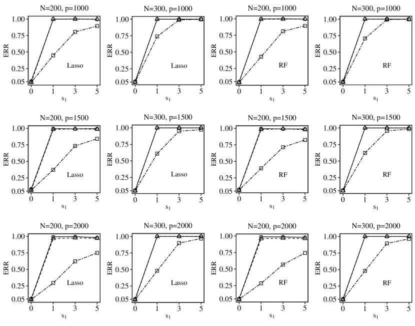
Figure 1: The empirical rejection rates of $\widetilde{T}_{n}$ ($\square$ with a two-dashed line), $T_{\mathrm{PE}}^{\mathrm{hard}}$ ($\triangle$ with a dashed line) and $T_{\mathrm{PE}}^{\mathrm{soft}}$ ($\circ$ with a solid line) against the sparsity level $s_{1}$ for Model 2 under different sample sizes and dimensions. “Lasso” and “RF” in figures represent that $\widehat{g}(\mathbf{Z}_{i})$ is obtained by Lasso and Random Forest, respectively.

In sum, our proposed power-enhanced test statistics have satisfactory performance. Firstly, $T_{\mathrm{PE}}^{\mathrm{hard}}$ and $T_{\mathrm{PE}}^{\mathrm{soft}}$ do not inflate the empirical size under $\mathbb{H}_{0}$, and still control the type-I error very well, which coincides with the theoretical result in Theorem 3.1. Secondly, the power-enhanced tests $T_{\mathrm{PE}}^{\mathrm{hard}}$ and $T_{\mathrm{PE}}^{\mathrm{soft}}$ substantially promote the testing power of $\widetilde{T}_{n}$, which echoes with the power enhancement property described in Theorem 3.2. Thirdly, the soft threshold $\delta_{k}^{\mathrm{soft}}$ prevails with higher power enhancement compared with the hard threshold $\delta_{k}^{\mathrm{hard}}$ in some cases. Further, the overall patterns for $\rho=0.3$ and $\rho=0.7$ are similar to those in Figure 1, and we thereby do not present these results to save space.

4.4 Study 3. Comparison with the maximum-type statistic

In this part, we compare our test statistics $\widetilde{T}_{n}$, $T_{\mathrm{PE}}^{\mathrm{hard}}$ and $T_{\mathrm{PE}}^{\mathrm{soft}}$ with the three-step testing procedure based on the studentized statistic in Zhang and Cheng, (2017), denoted as $T_{\mathrm{ST}}$. Here, we implement $T_{\mathrm{ST}}$ using R-package SILM, set the number of bootstrap replications as 500 and choose the splitting proportion of 30% for screening.

The computational expense of $T_{\mathrm{ST}}$ is high since it involves many penalized optimization implementations. Considering the computational limits, we only study Model 2 and set $(N,p,\rho)=(200,2000,0.5)$ under Scenarios 1-3. Additionally, we extend $s_{1}=\{1,3,5,7,9,11\}$ in Scenario 2 and $s_{1}=\{200,300,400,500,600,700\}$ in Scenario 3. From the aforementioned simulation results, it can be seen that Lasso and RF have similar performance, we thus just use Lasso in this part.

The comparison results for Model 2 is provided in Figure 2, which shows how the empirical reject rates of $\widetilde{T}_{n}$, $T_{\mathrm{PE}}^{\mathrm{hard}}$ and $T_{\mathrm{PE}}^{\mathrm{soft}}$ compare with $T_{\mathrm{ST}}$ at seven values of the sparsity level $s_{1}$. Note that the signal strength $c_{1}$ decreases with increasing $s_{1}$ since we set $c_{1}=1/s_{1}^{2/3}$ and $c_{1}=1/\sqrt{s_{1}}$ for sparse and dense alternatives, respectively. There are some findings. Firstly, the right panel in Figure 2 reveals that our proposed quadratic-form statistic achieves high testing power against dense alternatives. In contrast, the maximum-type method $T_{\mathrm{ST}}$ loses the detection of dense signals. Secondly, $\widetilde{T}_{n}$ lacks the ability to test sparse alternatives, especially $T_{\mathrm{ST}}$ has better performance than $\widetilde{T}_{n}$ when the sparsity level $s_{1}$ is small. However, the test performance of $T_{\mathrm{ST}}$ gradually decreases as the sparsity level $s_{1}$ increases (the signal strength $c_{1}$ decreases), even inferior to the quadratic-form statistic $\widetilde{T}_{n}$, because of weak signals. Thirdly, it is satisfactory that the proposed power-enhanced tests $T_{\mathrm{PE}}^{\mathrm{hard}}$ and $T_{\mathrm{PE}}^{\mathrm{soft}}$ substantially boost the power of $\widetilde{T}_{n}$ under sparse alternatives and remain high power for dense alternatives. Besides, the proposed power-enhanced tests always have higher power than $T_{\mathrm{ST}}$ in these settings.

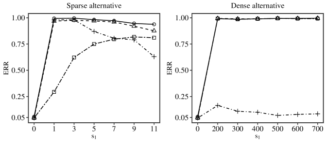
Figure 2: The empirical rejection rates of $\widetilde{T}_{n}$ ($\square$ with a two-dashed line), $T_{\mathrm{PE}}^{\mathrm{hard}}$ ($\triangle$ with a dashed line), $T_{\mathrm{PE}}^{\mathrm{soft}}$ ($\circ$ with a solid line) and $T_{\mathrm{ST}}$ ($+$ with a dot-dashed line) against the sparsity level $s_{1}$ for Model 2 under the sparse (left panel) and dense (right panel) case. Due to the computation limit, the results of $T_{\mathrm{ST}}$ are based on 200 replicates.

Overall, our simulation results demonstrate that the proposed procedures achieve controlled type-I errors and high powers, even when the testing and nuisance covariates are both ultrahigh-dimensional. When the signals are sparse, the power-enhanced test $T_{\mathrm{PE}}$ can greatly improve the performance of the quadratic-form test $\widetilde{T}_{n}$. The power-enhanced test $T_{\mathrm{PE}}$ then provides an innovative and straightforward approach suitable for sparse and dense cases simultaneously. Moreover, ML estimation is an effective tool for handling complex data structures.

5 Real data analysis

We analyze a dataset about riboflavin (vitamin B2) production rate with Bacillus Subtilis, which is a high-dimensional data set made publicly by Bühlmann et al., (2014). This data set attracts considerable attention and has been systematically analyzed by many authors, for instance, Meinshausen et al., (2009), Van de Geer et al., (2014), Javanmard and Montanari, (2014) and Yang et al., (2022). The dataset riboflavin can be obtained from the R-package hdi. It consists of $n=71$ observations of strains of Bacillus Subtilis. The predictors are the log-expression levels of $p=4088$ genes, and the response is the logarithm of the riboflavin production rate. Same to previous research papers, we standardize the predictors and response to be zero mean and unit variance.

Firstly, we use the sure independence screening procedure based on the distance correlation (DC-SIS, Li et al.,, 2012) to select genes that possibly impact the response. DC-SIS is implemented here using R-package VariableScreening. The genes selected are denoted as $\mathbf{X}$, and the other genes are denoted as $\mathbf{Z}$. Then two natural questions arise: (a) whether the selected genes $\mathbf{X}$ affect the response $Y$ given the other genes $\mathbf{Z}$; (b) whether the eliminated genes $\mathbf{Z}$ by the screening methods are indeed irrelevant to the response $Y$ given the other genes $\mathbf{X}$. Without loss of generality, we assume that the data set has the same structure as model (1.1). More specifically, we consider the following regression models,

$$Y=\mathbf{X}^{\top}\bm{\beta}_{\mathbf{X}}+g(\mathbf{Z})+\epsilon\quad\text{and}\quad Y=\mathbf{Z}^{\top}\bm{\beta}_{\mathbf{Z}}+g(\mathbf{X})+\epsilon,$$

for questions (a) and (b), respectively. We thereby consider two null hypotheses $\mathbb{H}_{0}:\bm{\beta}_{\mathbf{X}}=0$ and $\mathbb{H}_{0}^{\prime}:\bm{\beta}_{\mathbf{Z}}=0$ to check whether the chosen genes $\mathbf{X}$ contribute to the response and whether any significant genes remain in $\mathbf{Z}$.

Here we pick out the most important 200 genes ($\mathbf{X}$) by DC-SIS procedure. Since the sample size $n=71$ is small and the result of single data splitting may be unstable, we adopt $\widetilde{T}_{n}$, $T_{\mathrm{PE}}^{\mathrm{hard}}$ and $T_{\mathrm{PE}}^{\mathrm{soft}}$ for testing $\mathbb{H}_{0}$ and $\mathbb{H}_{0}^{\prime}$ with multiple data splitting illustrated in Section S2 in the Supplementary Material. We consider Lasso estimation in our methods. For comparison, we also apply $T_{\mathrm{ST}}$ to make significance tests. Table 3 shows the $p$-values for the considered hypotheses. For the test of $\mathbb{H}_{0}$, our three proposed tests reject the null hypothesis at the level of $\alpha=0.01$, while $T_{\mathrm{ST}}$ fails to reject it. The results for $\mathbb{H}_{0}^{\prime}$ suggest that the eliminated genes $\mathbf{Z}$ do not contain any genes that are significantly associated with the response.

Table 3: $p$-values of each test for riboflavin

	Method
Test	$\widetilde{T}_{n}$	$T_{\mathrm{PE}}^{\mathrm{hard}}$	$T_{\mathrm{PE}}^{\mathrm{soft}}$	$T_{\mathrm{ST}}$
$\mathbb{H}_{0}$	$<$0.001	$<$0.001	$<$0.001	0.056
$\mathbb{H}_{0}^{\prime}$	0.330	0.330	0.330	0.174

• Note. We adopt the multiple data splitting procedure with $M=30$ times splits.

6 Discussions and conclusions

In this paper, we develop testing procedures for ultrahigh-dimensional partially linear models. Our procedures allow the testing covariates and nuisance covariates to be both ultrahigh-dimensional and also allow unknown smooth function. To estimate the unknown smooth function, ML methods are used. We construct quadratic-form test statistics by adopting sample-splitting and cross-fitting. We establish the proposed test statistics’ asymptotic distributions under the null and local alternative hypotheses. To further improve the performance of proposed test statistics, we introduce power-enhanced tests. Two thresholding rules are introduced for the power-enhanced tests. We prove that the power-enhanced tests can still control the type-I error well, and have larger powers for either sparse or dense alternatives.

In this paper, we model the relationship between $\mathbf{X}$ and $Y$ linearly while allowing a flexible relationship between $\mathbf{Z}$ and $Y$. In near future, we aim to allow both flexible modelling of the relationships between $\mathbf{X}$ and $Y$ and between $\mathbf{Z}$ and $Y$. New theories and methods are required for this more general model.

Funding

The research is supported by National Natural Science Foundation of China (12071038) and Beijing Natural Science Foundation (1212004).

References

- Bühlmann et al., (2014) Bühlmann, P., Kalisch, M., and Meier, L. (2014). High-dimensional statistics with a view toward applications in biology. Annual Review of Statistics and Its Application, 1:255–278.
- Cai et al., (2023) Cai, L., Guo, X., Li, G., and Tan, F. (2023). Tests for high-dimensional single-index models. Electronic Journal of Statistics, 17(1):429–463.
- Chen et al., (2023) Chen, J., Li, Q., and Chen, H. Y. (2023). Testing generalized linear models with high-dimensional nuisance parameters. Biometrika, 110(1):83–99.
- Chen et al., (2019) Chen, S. X., Li, J., and Zhong, P.-S. (2019). Two-sample and ANOVA tests for high dimensional means. Annals of Statistics, 47(3):1443–1474.
- Chernozhukov et al., (2018) Chernozhukov, V., Chetverikov, D., Demirer, M., Duflo, E., Hansen, C., Newey, W., and Robins, J. (2018). Double/debiased machine learning for treatment and structural parameters. The Econometrics Journal, 21(1):C1–C68.
- Cui et al., (2018) Cui, H., Guo, W., and Zhong, W. (2018). Test for high-dimensional regression coefficients using refitted cross-validation variance estimation. Annals of Statistics, 46(3):958–988.
- Dezeure et al., (2017) Dezeure, R., Bühlmann, P., and Zhang, C.-H. (2017). High-dimensional simultaneous inference with the bootstrap. Test, 26(4):685–719.
- Du et al., (2021) Du, L., Guo, X., Sun, W., and Zou, C. (2021). False discovery rate control under general dependence by symmetrized data aggregation. Journal of the American Statistical Association, pages 1–15.
- Fan et al., (2012) Fan, J., Guo, S., and Hao, N. (2012). Variance estimation using refitted cross-validation in ultrahigh dimensional regression. Journal of the Royal Statistical Society: Series B (Statistical Methodology), 74(1):37–65.
- Fan et al., (2020) Fan, J., Li, R., Zhang, C.-H., and Zou, H. (2020). Statistical foundations of data science. Chapman & Hall.
- Fan et al., (2015) Fan, J., Liao, Y., and Yao, J. (2015). Power enhancement in high-dimensional cross-sectional tests. Econometrica, 83(4):1497–1541.
- Götze et al., (2021) Götze, F., Sambale, H., and Sinulis, A. (2021). Concentration inequalities for polynomials in -sub-exponential random variables. Electronic Journal of Probability, 26:1–22.
- Guo and Chen, (2016) Guo, B. and Chen, S. X. (2016). Tests for high dimensional generalized linear models. Journal of the Royal Statistical Society: Series B (Statistical Methodology), 78(5):1079–1102.
- Härdle et al., (2000) Härdle, W., Liang, H., and Gao, J. (2000). Partially linear models. Physica Heidelberg.
- Javanmard and Montanari, (2014) Javanmard, A. and Montanari, A. (2014). Confidence intervals and hypothesis testing for high-dimensional regression. Journal of Machine Learning Research, 15(82):2869–2909.
- Li et al., (2012) Li, R., Zhong, W., and Zhu, L. (2012). Feature screening via distance correlation learning. Journal of the American Statistical Association, 107(499):1129–1139.
- Liu et al., (2020) Liu, Y., Zhang, S., Ma, S., and Zhang, Q. (2020). Tests for regression coefficients in high dimensional partially linear models. Statistics and Probability Letters, 163:108772.
- Ma et al., (2021) Ma, R., Cai, T., and Li, H. (2021). Global and simultaneous hypothesis testing for high-dimensional logistic regression models. Journal of the American Statistical Association, 116(534):984–998.
- Meinshausen et al., (2009) Meinshausen, N., Meier, L., and Bühlmann, P. (2009). P-values for high-dimensional regression. Journal of the American Statistical Association, 104(488):1671–1681.
- Ning and Liu, (2017) Ning, Y. and Liu, H. (2017). A general theory of hypothesis tests and confidence regions for sparse high dimensional models. Annals of Statistics, 45(1):158–195.
- Van de Geer et al., (2014) Van de Geer, S., Bühlmann, P., Ritov, Y., and Dezeure, R. (2014). On asymptotically optimal confidence regions and tests for high-dimensional models. Annals of Statistics, 42(3):1166–1202.
- Vansteelandt and Dukes, (2022) Vansteelandt, S. and Dukes, O. (2022). Assumption-lean inference for generalised linear model parameters. Journal of the Royal Statistical Society: Series B (Statistical Methodology), 84(3):657–685.
- Wainwright, (2019) Wainwright, M. J. (2019). High-dimensional statistics: A non-asymptotic viewpoint. Cambridge University Press.
- Wang and Cui, (2017) Wang, S. and Cui, H. (2017). Generalized F-test for high dimensional regression coefficients of partially linear models. Journal of Systems Science and Complexity, 30(5):1206–1226.
- Wang and Cui, (2020) Wang, S. and Cui, H. (2020). Test for high dimensional regression coefficients of partially linear models. Communications in Statistics - Theory and Methods, 49(17):4091–4116.
- Xu et al., (2016) Xu, G., Lin, L., Wei, P., and Pan, W. (2016). An adaptive two-sample test for high-dimensional means. Biometrika, 103(3):609–624.
- Yang et al., (2022) Yang, W., Guo, X., and Zhu, L. (2022). Score function-based tests for ultrahigh-dimensional linear models. arXiv preprint arXiv:2212.08446.
- Yu et al., (2022) Yu, X., Li, D., Xue, L., and Li, R. (2022). Power-enhanced simultaneous test of high-dimensional mean vectors and covariance matrices with application to gene-set testing. Journal of the American Statistical Association, pages 1–14.
- Zhang and Zhang, (2014) Zhang, C.-H. and Zhang, S. S. (2014). Confidence intervals for low dimensional parameters in high dimensional linear models. Journal of the Royal Statistical Society: Series B (Statistical Methodology), 76(1):217–242.
- Zhang and Cheng, (2017) Zhang, X. and Cheng, G. (2017). Simultaneous inference for high-dimensional linear models. Journal of the American Statistical Association, 112(518):757–768.
- Zhao et al., (2023) Zhao, F., Lin, N., and Zhang, B. (2023). A new test for high-dimensional regression coefficients in partially linear models. Canadian Journal of Statistics, 51(1):5–18.
- Zhong and Chen, (2011) Zhong, P.-S. and Chen, S. X. (2011). Tests for high-dimensional regression coefficients with factorial designs. Journal of the American Statistical Association, 106(493):260–274.