The power spectrum of extended [C $\scriptstyle\rm II$] halos around high redshift galaxies

Abstract

ALMA observations have detected extended ($\simeq 10$ kpc) [C $\scriptstyle\rm II$] halos around high-redshift ($z\lower 2.15277pt\hbox{$\;\buildrel>\over{\sim}\;$}5$) star-forming galaxies. If such extended structures are common, they may have an impact on the line intensity mapping (LIM) signal. We compute the LIM power spectrum including both the central galaxy and the [C $\scriptstyle\rm II$] halo, and study the detectability of such signal in an ALMA LIM survey. We model the central galaxy and the [C $\scriptstyle\rm II$] halo brightness with a $\rm S\acute{e}rsic$+exponential profile. The model has two free parameters: the effective radius ratio $f_{R_{\rm e}}$, and the central surface brightness ratio, $f_{\Sigma}$, between the two components. [C $\scriptstyle\rm II$] halos can significantly boost the LIM power spectrum signal. For example, for relatively compact [C $\scriptstyle\rm II$] halos ($f_{\Sigma}=0.4$, $f_{R_{\rm e}}=2.0$), the signal is boosted by $\simeq 20$ times; for more extended and diffuse halos ($f_{\Sigma}=0.1,f_{R_{\rm e}}=6.0$), the signal is boosted by $\simeq 100$ times. For the ALMA ASPECS survey (resolution $\theta_{\rm beam}=1.13^{\prime\prime}$, survey area $\Omega_{\rm survey}=2.9\,\rm arcmin^{2}$) the [C $\scriptstyle\rm II$] power spectrum is detectable only if the deL14d [C $\scriptstyle\rm II$] - SFR relation holds. However, with an optimized survey ($\theta_{\rm beam}=0.232^{\prime\prime}$, $\Omega_{\rm survey}=2.0\,\rm deg^{2}$), the power spectrum is detectable for all the [C $\scriptstyle\rm II$] - SFR relations considered in this paper. Such a survey can constrain $f_{\Sigma}$ ($f_{R_{\rm e}}$) with a relative uncertainty of $\sim 15\%$ ($\sim 10\%$). A successful LIM experiment will provide unique constraints on the nature, origin, and frequency of extended [C $\scriptstyle\rm II$] halos, and the [C $\scriptstyle\rm II$] - SFR relation at early times.

1 Introduction

Cosmic reionization, as the last major phase transition of the Universe, is a direct consequence of the formation of the first luminous objects. Determining the properties of galaxies in the Epoch of Reionization (EoR) is crucial to understand structure formation and evolution (Dayal & Ferrara, 2018). However, our progress is hampered by the limited number of EoR sources that can be directly accessed via targeted observations. Such limitation is particularly severe for faint galaxies, which are thought to be the primary sources of ionizing photons (Robertson et al., 2015; Mitra et al., 2015; Castellano et al., 2016) but are far below the detection limits of the current surveys (Salvaterra et al., 2013).

Line intensity mapping (LIM) is emerging as an efficient tool to detect these faint galaxies. LIM measures the integrated emission of spectral lines from all galaxies and the intergalactic medium (IGM) (see a review by Kovetz et al., 2017). By measuring fluctuations in the line emission from early galaxies, one could expect to obtain valuable physical insights about the properties of these sources and their role in reionization. Finally, LIM can also be used to put stringent constraints on cosmological models (Kovetz et al., 2019; Schaan & White, 2021; Karkare et al., 2022; Bernal & Kovetz, 2022). For example, Gong et al. (2020) proposed to use the multipole moments of the redshift-space LIM power spectrum to constrain the cosmological and astrophysical parameters.

There are several spectral lines of interest for intensity mapping including HI 21 cm line (Chang et al., 2010; Salvaterra et al., 2013), CO rotational lines (Breysse et al., 2014; Mashian et al., 2015; Li et al., 2016), bright optical emission lines such as $\rm Ly\alpha$ and $\rm H\alpha$ (Salvaterra et al., 2013; Pullen et al., 2014; Comaschi & Ferrara, 2016; Gong et al., 2017; Silva et al., 2018) and the far-infrared (FIR) fine-structure lines (Gong et al., 2012; Uzgil et al., 2014; Silva et al., 2015; Yue et al., 2015; Serra et al., 2016; Yue & Ferrara, 2019).

Among these, the [C $\scriptstyle\rm II$] emission line with wavelength 157.7 $\mu$m, corresponding to the ${}^{2}P_{3/2}\rightarrow^{2}P_{1/2}$ forbidden transition of singly ionized carbon, is the brightest one in the FIR (Stacey et al., 1991), and a dominant coolant of the neutral ISM (Stacey et al., 1991; Wolfire et al., 2003) and dense photo-dissociation regions (PDR, Hollenbach & Tielens, 1999). Therefore, the [C $\scriptstyle\rm II$] line can be used to probe the properties of the ISM at high redshift (Capak et al., 2015; Pentericci et al., 2016; Knudsen et al., 2016; Carniani et al., 2017; Bakx et al., 2020; Matthee et al., 2020).

Notably, a tight relation between [C $\scriptstyle\rm II$] luminosity and star formation rate (SFR) is found from both observations (De Looze et al., 2014; Herrera-Camus et al., 2015; Schaerer et al., 2020) and simulations (Vallini et al., 2015; Olsen et al., 2017; Leung et al., 2020). Therefore, the [C $\scriptstyle\rm II$] emission lines can be used to trace the star formation across cosmic time, albeit at high redshift the scatter around the local relation increases (Carniani et al., 2018). Conveniently, at early epochs, the line is shifted into the (sub-)mm wavelength range, which is accessible to ground-based telescopes such as the Atacama Large Millimeter/sub-millimeter Array (ALMA).

With the advent of ALMA, a large number of galaxies with [C $\scriptstyle\rm II$] emission line at $z>4$ have been detected, boosting the studies of the obscured star formation at high redshift (Hodge & da Cunha, 2020). Among these, a stacking analysis of ALMA observed galaxies (Fujimoto et al., 2019) discovered extended, 10 kpc scale [C $\scriptstyle\rm II$] halos around high redshift galaxies, whose size is $\simeq 5$ times larger than the UV size of the central galaxy. Similar results have been reported in the following studies both in subsequent stacking analysis (Ginolfi et al., 2020; Fudamoto et al., 2022) and individual galaxies (Fujimoto et al., 2020; Herrera-Camus et al., 2021; Akins et al., 2022; Lambert et al., 2022; Fudamoto et al., 2023).

The existence of extended [C $\scriptstyle\rm II$] halos around normal star-forming galaxies opens new perspectives for early metal enrichment. However, the physical origin of [C $\scriptstyle\rm II$] halos is still not clear. Possible scenarios include satellite galaxies, extended PDR or HII regions, cold streams, and outflows. These are discussed in Fujimoto et al. (2019). Indeed, the supernova-driven cooling outflow model explored by Pizzati et al. (2020); Pizzati et al. (2023) successfully produces the extended [C $\scriptstyle\rm II$] halo, their model also indicates that outflows are widespread phenomena in high-z galaxies, but the extended [C $\scriptstyle\rm II$] halos for low-mass galaxies are likely too faint to be detected with present levels of sensitivity. The outflow scenario is also supported by Ginolfi et al. (2020), who found outflow signatures in the stacking analysis of [C $\scriptstyle\rm II$] emission detected by ALMA in 50 main sequence star-forming galaxies at $4<z<6$. Fujimoto et al. (2020) also suggested that the star-formation-driven outflow is the most likely origin of the [C $\scriptstyle\rm II$] halos. Finally, Herrera-Camus et al. (2021) found evidence of outflowing gas, which may be responsible for the production of extended [C $\scriptstyle\rm II$] halos. On the other hand, Heintz et al. (2023) use [C $\scriptstyle\rm II$] emission as a proxy to infer the metal mass in the interstellar medium (ISM) of galaxies, and find that the majority of metals produced at $z\gtrsim 5$ are confined to the ISM, disfavour efficient outflow processes at these redshifts, they claim extended [C $\scriptstyle\rm II$] halos trace the extended neutral gas reservoirs of high-z galaxies. In any case, if [C $\scriptstyle\rm II$] halos are common in high redshift normal star-forming galaxies, they could leave a distinct imprint in LIM experiments.

In this paper, we aim to investigate the effects of extended [C $\scriptstyle\rm II$] halos on the LIM signal and their detectability. We first construct the [C $\scriptstyle\rm II$] halo model and compute the intensity mapping power spectrum of high redshift galaxy systems when both the central galaxy and extended [C $\scriptstyle\rm II$] halo are considered. Then we analyze the detectability of the signal in the ALMA intensity mapping survey and a proposed optimized survey. The paper is organized as follows: We outline our method in Section 2. Results, including the power spectrum signal and its signal-to-noise ratio (S/N) estimation, are presented in Section 3. We finally summarize the results and give a discussion in Section 4.

2 Method

In the following, we describe our model to derive the LIM signal when both central galaxies and [C $\scriptstyle\rm II$] halos are considered. We start by constructing the extended [C $\scriptstyle\rm II$] halo model, and the relations between central galaxy [C $\scriptstyle\rm II$] luminosity, extended [C $\scriptstyle\rm II$] halo luminosity, and dark matter halo mass. We then compute the intensity mapping power spectrum, including one-halo and two-halo terms, and the shot noise term. Finally, we introduce the method to estimate the signal-to-noise ratio of the [C $\scriptstyle\rm II$] power spectrum, given the LIM survey parameters.

2.1 [C $\scriptstyle\rm II$] halo model

To compute the clustering term of the power spectrum, the first step is to model the [C $\scriptstyle\rm II$] radial surface brightness of the central galaxy and the extended halo. For this, we use a combined $\rm S\acute{e}rsic$+exponential model, where the central galaxy is described by the $\rm S\acute{e}rsic$ model (Sérsic, 1963; Sersic, 1968) while the extended [C $\scriptstyle\rm II$] halo is described by the exponential function (Fujimoto et al., 2019; Akins et al., 2022).

The [C $\scriptstyle\rm II$] radial surface brightness of the central galaxy writes

$$\Sigma_{\rm CII,g}(R)=C_{\rm g}\exp\left[-b_{n}\left(\frac{R}{R_{\rm e,g}}\right)^{1/n}\right],$$ (1)

where $C_{\rm g}$ is the central surface brightness, $R$ is the projected distance to the source centre in the plane-of-sky, $n$ is the $\rm S\acute{e}rsic$ index, and $R_{\rm e,g}$ is the effective radius containing half of the integrated brightness. The term $b_{n}$ is a function of $n$. It is obtained by solving the equation $\Gamma(2n)=2\gamma(2n,b_{n})$, where $\Gamma(2n)$ is the Gamma function, $\gamma(2n,b_{n})=\int^{b_{n}}_{0}t^{2n-1}e^{-t}dt$ is the lower incomplete gamma function.

In the stacking analysis by Fujimoto et al. (2019), the central galaxies are well fitted by $\rm S\acute{e}rsic$ model with $n=1.2$ and $R_{\rm e,g}=1.1\,\rm kpc$. This is consistent with the rest-frame optical and UV sizes measured by Shibuya et al. (2015), who obtain a nearly constant value of $R_{\rm e,g}/R_{\rm vir}=1.0\%-3.5\%$ for $z=0-8$, where $R_{\rm vir}$ is the dark matter halo virial radius. Following these results, we adopt $n=1.2$ and fix $R_{\rm e,g}=0.03R_{\rm vir}$.

For the extended [C $\scriptstyle\rm II$] halo, the surface brightness has the exponential form

$$\Sigma_{\rm CII,h}(R)=C_{\rm h}\exp\left[-b_{1}\frac{R}{R_{\rm e,h}}\right],$$ (2)

where $b_{1}$ is the $b_{n}$ for $n=1$, $C_{\rm h}$ is the surface brightness at the center and the $R_{\rm e,h}$ is the effective radius of the [C $\scriptstyle\rm II$] halo. We further assume $C_{\rm h}=f_{\Sigma}C_{\rm g}$ and $R_{\rm e,h}=f_{R_{\rm e}}R_{\rm e,g}$, where the ratios $f_{\Sigma}$ and $f_{R_{\rm e}}$ are two free parameters in our work.

With the above surface brightness profiles, the [C $\scriptstyle\rm II$] luminosity for the central galaxy

$$L_{\rm CII,g} =\int 2\pi R\Sigma_{\rm CII,g}(R)dR$$

$$=2\pi C_{\rm g}\frac{n\Gamma(2n)}{(b_{n})^{2n}}R_{\rm e,g}^{2},$$ (3)

and for the extended [C $\scriptstyle\rm II$] halo

$$L_{\rm CII,h} =\int 2\pi R\Sigma_{\rm CII,h}(R)dR$$

$$=2\pi C_{\rm h}\frac{\Gamma(2)}{(b_{1})^{2}}R_{\rm e,h}^{2}.$$ (4)

Since restricted by the sensitivity of the telescope in previous observations, the observed [C $\scriptstyle\rm II$] luminosity in deriving the [C $\scriptstyle\rm II$] - SFR relation is likely dominated by central galaxies. Moreover, as noted by Fujimoto et al. (2019), to fully capture the extended [C $\scriptstyle\rm II$] halos, additional mechanisms not involved in previous simulations are required. Therefore, we consider the previously predicted [C $\scriptstyle\rm II$] - SFR relations (both by observations and by simulations ) do not account for (or at least significantly underestimate) the extended [C $\scriptstyle\rm II$] halo contribution. For clarification, we shall use $L_{\rm CII,SFR}-{\rm SFR}$ to denote the relations in the following of this work, where $L_{\rm CII,SFR}$ is the [C $\scriptstyle\rm II$] luminosity derived from the previously [C $\scriptstyle\rm II$] - SFR relations, see next subsection. We find the normalization by assigning $L_{\rm CII,g}\approx L_{\rm CII,SFR}$. Then

$$C_{\rm g}=\frac{(b_{n})^{2n}}{2\pi n\Gamma(2n)R_{\rm e,g}^{2}}L_{\rm CII,SFR}.$$ (5)

Then the [C $\scriptstyle\rm II$] halo luminosity is also derived from the $L_{\rm CII,SFR}$ via

$$L_{\rm CII,h}=f_{\Sigma}f_{R_{\rm e}}^{2}\frac{(b_{n})^{2n}}{(b_{1})^{2}}\frac{\Gamma(2)}{n\Gamma(2n)}L_{\rm CII,SFR},$$ (6)

and when $n=1.2$ it is reduced to

$$L_{\rm CII,h}\simeq 2.24f_{\Sigma}f_{R_{\rm e}}^{2}L_{\rm CII,SFR}.$$ (7)

We further assume that the profile is spherically symmetric, and perform a deprojection of the above surface density to obtain the 3D brightness profiles for the two components, $\rho_{\rm CII,g}(r)$ and $\rho_{\rm CII,h}(r)$. This is given in Appendix A. The total 3D brightness profile is the sum of the two components

$$\rho_{\rm CII}(r)=\rho_{\rm CII,g}(r)+\rho_{\rm CII,h}(r),$$ (8)

and we truncate it at $R_{\rm vir}$. Then, the normalized Fourier transform of the profile in a dark matter halo of mass $M_{\rm vir}$,

$$u_{\rm CII}(k|M_{\rm vir})=\frac{\int^{R_{\rm vir}}_{0}dr\,4\pi r^{2}\frac{\sin{kr}}{kr}\rho_{\rm CII}(r)}{\int^{R_{\rm vir}}_{0}dr\,4\pi r^{2}\rho_{\rm CII}(r)},$$ (9)

which is used to compute the one-halo and two-halo terms of the power spectrum. The luminosity density profiles of the central galaxy and [C $\scriptstyle\rm II$] halo are shown in the left panel of Fig. 1. We take $M_{\rm vir}=10^{12}~{}M_{\odot}$ at $z=6$, $f_{\Sigma}=0.4$ and $f_{R_{\rm e}}=2.0,6.0,10.0$. In the right panel of Fig. 1 we show the Fourier transform of the profiles for different $f_{R_{\rm e}}$.

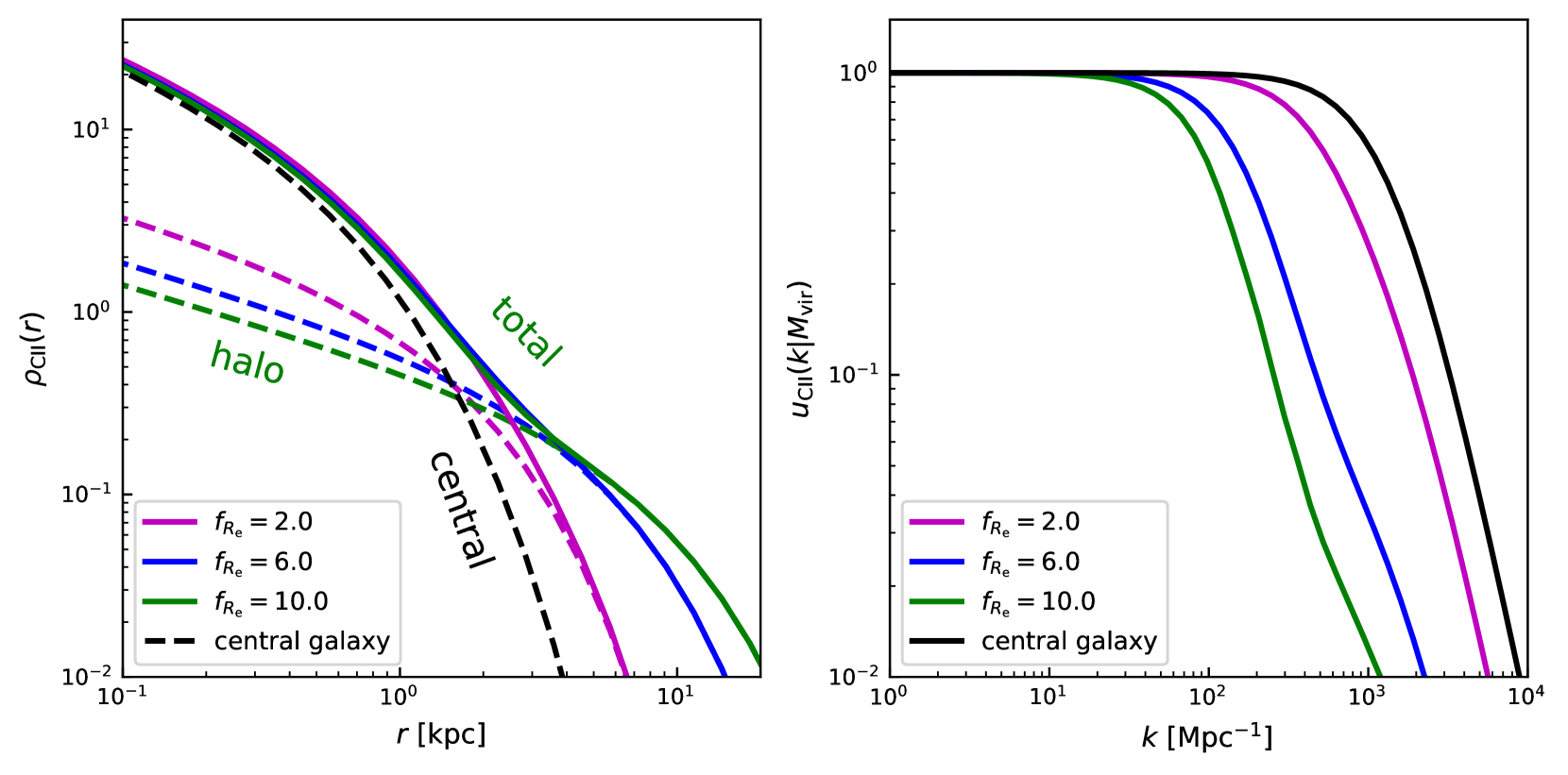
Figure 1: Left: The radial profile of a [C $\scriptstyle\rm II$] halo in dark matter halo with mass $M_{\rm vir}=10^{12}\,\rm M_{\odot}$. We fix [C $\scriptstyle\rm II$] halo parameter $f_{\Sigma}=0.4$ and vary the effective radius ratios $f_{R_{\rm e}}$. The black dashed line is the profile of the central galaxy. The green, blue, and magenta dashed lines are the profiles of the [C $\scriptstyle\rm II$] halo part with $f_{R_{\rm e}}=[2.0,6.0,10.0]$ respectively. The solid lines represent the sum of the central galaxy and [C $\scriptstyle\rm II$] halo components. Right: The corresponding normalized Fourier transform of the [C $\scriptstyle\rm II$] halo profile with different effective radius ratios $f_{R_{\rm e}}$.

2.2 The [C $\scriptstyle\rm II$] - dark matter halo mass relation

To derive the $L_{\rm CII,SFR}-M_{\rm vir}$ relation, we first use the abundance matching method to get $\rm SFR-M_{\rm vir}$ relation. Following Yue et al. (2015), we start from the observed (dust-attenuated) galaxy UV luminosity function (LF), which can be described by a Schechter function (Schechter, 1976)

$$\frac{dn}{dM_{\rm UV}^{\rm obs}} =0.4\ln(10)\Phi^{*}10^{-0.4(M_{\rm UV}^{\rm obs}-M_{\rm UV}^{*})(\alpha+1)}$$ (10)

$$\times\exp{[-10^{-0.4(M_{\rm UV}^{\rm obs}-M_{\rm UV}^{*})}]},$$

where the $M_{\rm UV}^{\rm obs}$ is the dust-attenuated absolute UV magnitude, and the redshift-dependent parameters are taken from Bouwens et al. (2015),

$$M_{\rm UV}^{*} =-20.95+0.01(z-6),$$ (11)

$$\Phi^{*} =0.47\times 10^{-3-0.27(z-6)},$$

$$\alpha =-1.87-0.10(z-6).$$

Considering dust attenuation, the intrinsic absolute UV magnitude becomes

$$M_{\rm UV}=M_{\rm UV}^{\rm obs}-A_{\rm UV},$$ (12)

where the UV dust attenuation is parameterized as

$$A_{\rm UV}=C_{1}+C_{0}\beta\ (A_{\rm UV}\geq 0);$$ (13)

we set the coefficients $C_{0}=2.10$ and $C_{1}=4.85$, following Koprowski et al. (2018). Finally, the UV spectral slope $\beta$ is fitted by Bouwens et al. (2015)

$$\beta=\beta_{\rm 0}+\frac{d\beta}{dM_{\rm 0}}(M_{\rm UV}^{\rm obs}-M_{\rm 0}),$$ (14)

with a redshift dependence given by

$$\beta_{0}=-1.97-0.06(z-6),$$ (15)

$$\frac{d\beta}{dM_{\rm UV}}=-0.18-0.03(z-6).$$

The intrinsic UV LF is related to the observed UV LF by

$$\frac{dn}{dM_{\rm UV}}=\frac{dn}{dM_{\rm UV}^{\rm obs}}\frac{dM_{\rm UV}^{\rm obs}}{dM_{\rm UV}}.$$ (16)

By assuming that the most massive galaxies occupy the most massive dark matter halos, we use the abundance matching method

$$\int_{M_{\rm UV}}\frac{dn}{dM_{\rm UV}}dM_{\rm UV}=\int_{M_{\rm vir}}\frac{dn}{dM_{\rm vir}}dM_{\rm vir},$$ (17)

to derive the intrinsic absolute UV magnitude and dark matter halo mass relation. To get the ${\rm SFR}-M_{\rm vir}$ relation, we assume that the intrinsic UV luminosity scales with the SFR (Kennicutt, 1998)

$${\rm SFR}=K_{\rm UV}L_{\rm UV},$$ (18)

where $K_{\rm UV}=0.7\times 10^{-28}\,\rm M_{\odot}\ yr^{-1}/(erg\ s^{-1}\ Hz^{-1})$ (Bruzual & Charlot, 2003) for a Chabrier (2003) stellar initial mass function (IMF), metallicity in the range $0.005-0.4\ Z_{\odot}$, and stellar age $>100\,\rm Myr$; we ignore the scatter on $K_{\rm UV}$ as discussed by Yue & Ferrara (2019).

The final step to get the $L_{\rm CII,SFR}-M_{\rm vir}$ relation involves the $L_{\rm CII,SFR}-\rm SFR$ relation. This can be parameterized as

$$\log L_{\rm CII,SFR} =\log\bar{L}_{\rm CII,SFR}\pm\sigma_{\rm L}$$ (19)

$$=\log A+\gamma\log\rm{SFR}\pm\sigma_{L},$$

where SFR is in units of $\rm M_{\rm\odot}\ {\rm yr}^{-1}$, and $L_{\rm CII,SFR}$ in units of $\rm L_{\odot}$. We adopt six different $L_{\rm CII,SFR}-\rm SFR$ relations to compute the power spectrum in our model. These relations are described in the following.

By combining a semi-analytical model of galaxy formation with the photo-ionisation code CLOUDY (Ferland et al., 2013, 2017) to compute the [C $\scriptstyle\rm II$] luminosity for a large number of galaxies at $z\geq 4$, Lagache et al. (2018, hereafter L18) reproduced the $L_{\rm CII,SFR}-\rm SFR$ relation observed in high-$z$ star-forming galaxies. They found a mild evolution of the $L_{\rm CII,SFR}-\rm SFR$ relation with redshift from $z=4$ to $z=7.6$,

$$\log L_{\rm CII,SFR}=(7.1-0.07z)+(1.4-0.07z)\log(\rm SFR),\rm$$ (20)

with a scatter of about 0.5 dex.

De Looze et al. (2014) analysed the $L_{\rm CII,SFR}-\rm SFR$ relation for low-metallicity dwarf galaxies based on Herschel observations (Madden et al., 2013) and found a local relation with $\log A=7.16$, $\gamma=1.25$ and 0.5 dex scatter (hereafter deL14d), i.e.

$$\log L_{\rm CII,SFR}=7.16+1.25\log\rm SFR,$$ (21)

De Looze et al. (2014) also obtained $\log A=7.22$, $\gamma=0.85$ and 0.3 dex scatter (hereafter deL14$z$) for high-$z$ samples with $z=0.59-6.60$.

$$\log L_{\rm CII,SFR}=7.22+0.85\log\rm SFR$$ (22)

Olsen et al. (2017) obtained $\log A=6.69$ and $\gamma=0.58$, with a scatter of $\sim 0.15$ dex (here after O17) by combining cosmological zoom simulations of galaxies with SÍGAME (Olsen et al., 2015) to model [C $\scriptstyle\rm II$] emissions from 30 main-sequence galaxies at $z\sim 6$,

$$\log L_{\rm CII,SFR}=(6.69\pm 0.10)+(0.58\pm 0.11)\log\rm SFR.$$ (23)

This is consistent with Leung et al. (2020) who predict $\log A=6.82$ and $\gamma=0.66$, based on cosmological hydrodynamics simulations using the SIMBA suite plus radiative transfer calculations via an updated version of SÍGAME.

Vallini et al. (2015) combined high-resolution, radiative transfer cosmological simulations with a subgrid multiphase model of the ISM to model the [C $\scriptstyle\rm II$] emissions from diffuse neutral gas and PDRs. By considering a physically-motivated metallicity, they found $L_{\rm CII,SFR}-\rm SFR$ relation both depends on the SFR and metallicity and can be fitted by

$$\log{L}_{\rm CII,SFR} =7.0+1.2\log(\rm SFR)+0.021\log(Z)$$ (24)

$$+0.012\log(\rm SFR)\log(Z)-0.74\log^{2}(Z).$$

For $Z=0.2\,\rm Z_{\odot}$, we obtain $\log A=6.62$ and $\gamma=1.19$ (here after V15).

Schaerer et al. (2020), using 118 galaxies at $4.4<z<5.9$ from the ALMA ALPINE Large Program (Le Fèvre et al., 2020), obtain

$$\log L_{\rm CII,SFR}=\left(6.61\pm 0.2\right)+\left(1.17\pm 0.12\right)\log\rm SFR,$$ (25)

with a scatter of $\sim 0.28$ dex (here after S20).

The parameters of the six $L_{\rm CII,SFR}-{\rm SFR}$ relations adopted are summarized in Tab. 1. Since the observed $\sigma_{\rm L}$ involves both the observational uncertainties and the intrinsic scatters, and the simulated $\sigma_{\rm L}$ might be limited by the method of modelling the input physical properties scattering, for simplicity in this work we ignore the $\sigma_{\rm L}$ and simply use $\log L_{\rm CII,SFR}=\log A+\gamma\log{\rm SFR}$ in the following. We plot the corresponding $L_{\rm CII,SFR}-M_{\rm vir}$ relations in Fig. 2.

Table 1: Summary of $L_{\rm CII,SFR}-\rm SFR$ relation parameters adopted in our model.

model	$\log\ A$	$\gamma$	$\sigma_{\rm L}$	Redshift	References
L18	6.68	0.98	0.60	6	Lagache et al. (2018)
deL14d	7.16	1.25	0.5	Local	De Looze et al. (2014)
deL14z	7.22	0.85	0.3	6.6	De Looze et al. (2014)
O17	6.69	0.58	0.15	6	Olsen et al. (2017)
V15	6.62	1.19	0.4	6.6	Vallini et al. (2015)
S20	6.61	1.17	0.28	4.4-5.9	Schaerer et al. (2020)

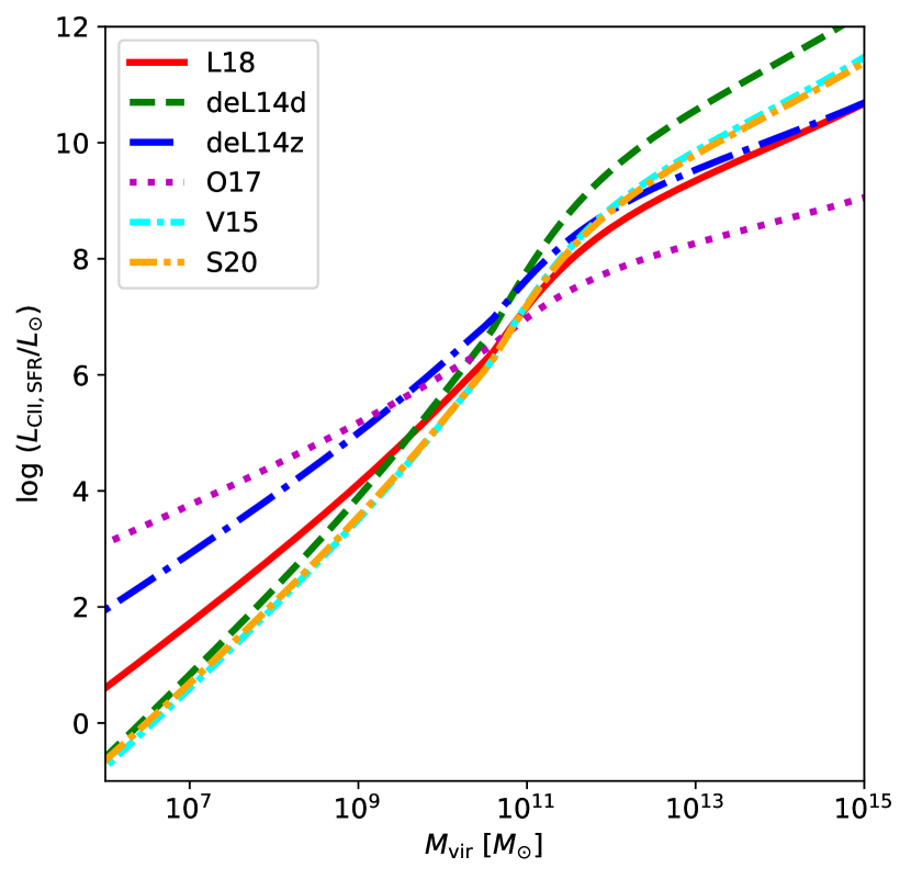
Figure 2: The $L_{\rm CII,SFR}-M_{\rm vir}$ relation obtained from Abundance Matching method for six $L_{\rm CII,SFR}-\rm SFR$ relations.

2.3 Modeling the power spectrum

Since galaxies are biased and discrete tracers of the dark matter density fluctuations, basically the LIM power spectrum comprises clustering and shot noise components (Kovetz et al., 2017). The clustering term describes the large-scale clustering nature of galaxies and the shot noise term originates from the Poisson fluctuations of galaxy numbers. In the halo model framework (Cooray & Sheth, 2002), the clustering term can be split into one-halo term and two-halo term, which arise from the correlation within halos and between halos, respectively (Moradinezhad Dizgah et al., 2022). The LIM power spectrum writes:

$$P_{\rm CII}(k,z) =P_{\rm CII}^{\rm CL}(k,z)+P_{\rm CII}^{\rm SN}(z)$$ (26)

$$=P_{\rm CII}^{\rm 1h}(k,z)+P_{\rm CII}^{\rm 2h}(k,z)+P_{\rm CII}^{\rm SN}(z),,$$

where the shot noise $P_{\rm CII}^{\rm SN}(z)$ is generally independent of $k$. The one-halo term $P_{\rm CII}^{\rm 1h}(k,z)$ and the two-halo term $P_{\rm CII}^{\rm 2h}(k,z)$ depend on the large-scale structure, the normalized Fourier transform of the [C $\scriptstyle\rm II$] halo profile and the $L_{\rm CII,SFR}-M_{\rm vir}$ relation.

Analogous to the halo model (Cooray & Sheth, 2002) which assumes the correlation is tightly related to the (density or light) distribution profile within dark matter halos, the one-halo term (Moradinezhad Dizgah et al., 2022) is

$$P_{\rm CII}^{\rm 1h}(k,z)=\int dM_{\rm vir}\frac{dn}{dM_{\rm vir}}u_{\rm CII}(k|M_{\rm vir})^{2}\left[\frac{L_{\rm CII}(M_{\rm vir},z)}{4\pi D^{2}_{\rm L}}y(z)D_{\rm c}^{2}\right]^{2}$$ (27)

$$=\left(\frac{c}{4\pi\nu_{\rm CII}H(z)}\right)^{2}\int dM_{\rm vir}\frac{dn}{dM_{\rm vir}}[L_{\rm CII}(M_{\rm vir},z)u_{\rm CII}(k|M_{\rm vir})]^{2},$$

and two-halo term (Moradinezhad Dizgah et al., 2022) is

$$P_{\rm CII}^{\rm 2h}(k,z) =\left(\int dM_{\rm vir}\frac{dn}{dM_{\rm vir}}u_{\rm CII}(k|M_{\rm vir})\right)^{2}\left[\frac{L_{\rm CII}(M_{\rm vir},z)}{4\pi D^{2}_{\rm L}}y(z)D_{\rm c}^{2}\right]^{2}$$ (28)

$$=\left(\int dM_{\rm vir}\frac{dn}{dM_{\rm vir}}L_{\rm CII}(M_{\rm vir},z)u_{\rm CII}(k|M_{\rm vir})b_{\rm SMT}(M_{\rm vir},z)\right)^{2}$$

$$\times\left(\frac{c}{4\pi\nu_{\rm CII}H(z)}\right)^{2}P(k,z).$$

$D_{\rm L}$ is the luminosity distance and $D_{\rm c}$ is the comoving distance to redshift $z$. $y(z)=c(1+z)/[\nu_{0}H(z)]$ is the derivative of the comoving radial distance with respect to the observed frequency $\nu_{0}$, which is related to the rest-frame frequency of [C $\scriptstyle\rm II$] line as $\nu_{0}=\nu_{\rm CII}/(1+z)$; $c$ is the light speed and $H(z)$ is the Hubble parameter. We adopt the Sheth-Tormen form (Sheth & Tormen, 1999) of the halo mass function $dn/dM_{\rm vir}$, the Eisenstein & Hu (1999) form of the linear matter power spectrum $P(k,z)$, and the Sheth et al. (2001) form of dark matter halo bias $b_{\rm SMT}(M_{\rm vir},z)$. $L_{\rm CII}(M_{\rm vir},z)=L_{\rm CII,g}+L_{\rm CII,h}$ is the [C $\scriptstyle\rm II$] luminosity of the dark matter halo with mass $M_{\rm vir}$, including the central galaxy and the extended [C $\scriptstyle\rm II$] halo.

Finally, the Poissonian shot noise, arising from the discrete nature of dark matter halos, can be computed as (Uzgil et al., 2014)

$$P_{\rm CII}^{\rm SN}(z)=\left(\frac{c}{4\pi\nu_{\rm CII}H(z)}\right)^{2}\int dM_{\rm vir}\frac{dn}{dM_{\rm vir}}L_{\rm CII}^{2}(M_{\rm vir},z)$$ (29)

The integration of Eqs. (27, 28 & 29) is performed between $M_{\rm min}$ and $M_{\rm max}$. We set $M_{\rm min}=10^{8}\,\rm M_{\odot}$, which is roughly the atomic cooling threshold (the virial mass corresponding to virial temperature $10^{4}$ K) at redshift 6. This is the minimum mass that can sustain persistent star formation activity. Generally, the number density of dark matter halos with mass $M_{\rm vir}$ can be approximated as $\bar{n}\sim M_{\rm vir}\frac{dn}{dM_{\rm vir}}=\frac{dn}{d\ln M_{\rm vir}}$. Suppose the survey volume is $V_{\rm survey}$, then in such volume the mean number of dark matter halos with mass $M_{\rm vir}$ is just

$$\bar{n}V_{\rm survey}\sim\frac{dn}{d\ln M_{\rm vir}}V_{\rm survey}.$$ (30)

In $V_{\rm survey}$, the probability to find at least one dark matter halo with mass $\sim M_{\rm vir}$ is $G(\geq 1|\bar{n}V_{\rm survey})$, where $G$ is the cumulative Poisson probability with mean value $\bar{n}V_{\rm survey}$. We obtain $M_{\rm max}$ by solving the equation $G(\geq 1|\bar{n}V_{\rm survey})=0.5$, which means in the volume $V_{\rm survey}$ the contribution from dark matter halos whose existence probability smaller than $50\%$ is excluded. This is to avoid such bright and rare objects biasing our results. When $V_{\rm survey}=10^{6}~{}$Mpc³, $M_{\rm max}\sim 2.2\times 10^{12}\,\rm M_{\rm\odot}$ at redshift 6.

Let’s interpret the one-halo term, two-halo term, and shot noise of the [C $\scriptstyle\rm II$] power spectrum more physically. Since the mean [C $\scriptstyle\rm II$] specific intensity is (Gong et al., 2011)

$$\bar{I}_{\rm CII}(z)=\int dM_{\rm vir}\frac{dn}{dM_{\rm vir}}\left[\frac{L_{\rm CII}(M_{\rm vir},z)}{4\pi D^{2}_{\rm L}}y(z)D_{\rm c}^{2}\right],$$ (31)

so the one-halo term can be interpreted as the auto-correlations of the [C $\scriptstyle\rm II$] light distribution within dark matter halos, weighed by the square of their contribution to the mean [C $\scriptstyle\rm II$] specific intensity. On the other hand, at scales much larger than the dark matter halo size, the two-halo term has the approximation form

$$P_{\rm CII}^{\rm 2h}(k,z)\approx\bar{I}_{\rm CII}^{2}(z)\bar{b}_{\rm SMT}^{2}P(k,z),$$ (32)

where $\bar{b}_{\rm SMT}$ is the mean halo bias. So the two-halo term actually describes the large-scale power spectrum of the dark matter halos weighted by the square of mean [C $\scriptstyle\rm II$] specific intensity. Regarding the shot noise, it has the approximation

$$P_{\rm CII}^{\rm SN}(z)\approx\bar{I}^{2}_{\rm CII}(z)\frac{1}{\bar{n}},$$ (33)

where $\bar{n}$ is the number density of dark matter halos that have a dominant contribution in the shot noise. Clearly, this approximation shows that shot noise is actually the Poisson fluctuations of the dark matter halos, weighted by the square of the mean [C $\scriptstyle\rm II$] specific intensity.

2.4 The signal-to-noise ratio estimation

For a LIM survey, the smallest and largest accessible $k$ modes for probing the fluctuations are determined by the survey volume and the resolution (angular resolution $\delta\theta$ and frequency resolution $\delta\nu_{0}$). The survey volume is determined by the redshift of the target, the survey area $\Omega_{\rm survey}$, and the bandwidth coverage $\Delta\nu_{0}$.

Along the line of sight, the spatial resolution corresponds to the frequency resolution (Bull et al., 2015),

$$\Delta r_{\rm\parallel,min}\approx\frac{c(1+z)}{H(z)}\frac{\delta\nu_{0}}{\nu_{0}};$$ (34)

while the largest spatial across corresponds to the bandwidth,

$$\Delta r_{\rm\parallel,max}\approx\frac{c(1+z)}{H(z)}\frac{\Delta\nu_{0}}{\nu_{0}}.$$ (35)

The tangential spatial resolution corresponds to the synthesized beam size $\Omega_{\rm beam}$

$$\Delta r_{\rm\perp,min}\approx D_{\rm c}(z)\sqrt{\Omega_{\rm beam}},$$ (36)

and the largest spatial across corresponds to the survey area $\Omega_{\rm survey}$

$$\Delta r_{\rm\perp,max}\approx D_{\rm c}(z)\sqrt{\Omega_{\rm survey}}.$$ (37)

Then, along and perpendicular to the line of sight, the smallest and largest $k$ modes that can be detected by the survey are (Uzgil et al., 2019),

$$k_{\rm\parallel,min}=\frac{2\pi}{\Delta r_{\rm\parallel,max}}\ {\rm and}\ k_{\rm\parallel,max}=\frac{1}{2}\frac{2\pi}{\Delta r_{\rm\parallel,min}},$$ (38)

$$k_{\rm\perp,min}=\frac{2\pi}{\Delta r_{\rm\perp,max}}\ {\rm and}\ k_{\rm\perp,max}=\frac{1}{2}\frac{2\pi}{\Delta r_{\rm\perp,min}}.$$ (39)

Finally, the survey detects the isotropic power spectrum in the range $k_{\rm min}<k<k_{\rm max}$, for which $k_{\rm min}\approx\sqrt{k^{2}_{\parallel,\rm min}+k^{2}_{\perp,\rm min}}$ and $k_{\rm max}\approx\sqrt{k^{2}_{\parallel,\rm max}+k^{2}_{\perp,\rm max}}$.

The variance of the power spectrum measured in the above LIM survey is

$$\sigma_{P}^{2}(k)=\frac{1}{N_{\rm m}(k)}\left[P_{\rm CII}(k,z)+P_{\rm N}W^{-2}_{\rm res}(k)\right]^{2},$$ (40)

where $W_{\rm res}(k)$ is the window function that denotes the rapid decline of the measured power spectrum below the resolution (Lidz et al., 2011; Lidz & Taylor, 2016; Seo et al., 2010; Battye et al., 2013; Bernal et al., 2019). In principle $\Delta r_{\parallel,\rm min}$ can be very different from $\Delta r_{\perp,\rm min}$, so the window function for $k_{\parallel}$ and $k_{\perp}$ should be different (Lidz et al., 2011; Lidz & Taylor, 2016; Bernal et al., 2019; Bernal & Kovetz, 2022). In that case, at the small scale, the power spectrum is no longer isotropic and the cylinder power spectrum should be used. However, in this paper, we only investigate the isotropic power spectrum, we implicitly assume that the $\Delta r_{\parallel,\rm min}$ are comparable to the $\Delta r_{\perp,\rm min}$. For this reason, we adopt the approximation (Battye et al., 2013)

$$W_{\rm res}(k)\approx\exp\left[-\frac{1}{2}k^{2}D^{2}_{\rm c}(z)\frac{\Omega_{\rm beam}}{4}\right].$$ (41)

In principle, there is another window function that describes the power spectrum decline beyond the finite survey volume (Bernal et al., 2019). In our calculations we do not consider such a window function, instead, we consider the power spectrum at $k>k_{\rm min}$ is fully measured and at $k<k_{\rm min}$ is fully missed, for which $k_{\rm min}$ is set by the survey volume. This is equivalent to adopting a sharp $k$ cutoff step function as the window function. Although this may not be the real case, it will just have quite limited effects on the results, because the contributions to signal-to-noise ratio and parameter constraints from $k$ modes close to $k_{\rm min}$ are small, see the results in Sec. 3.2.

In Eq. (40), $P_{\rm N}$ is the instrumental noise power spectrum. $N_{\rm m}(k)$ is the number of $k$ modes sampled by a survey in the $k$-bin, which is estimated (Chung et al., 2020) by

$$N_{\rm m}(k)\approx 2\pi k^{3}d\ln{k}\frac{V_{\rm survey}}{(2\pi)^{3}},$$ (42)

where $d\ln k$ is the relative width of the selected $k$-bin, and $V_{\rm survey}$ is the survey volume,

$$V_{\rm survey}\approx D_{\rm c}^{2}(z)\Omega_{\rm survey}\left[\frac{c(1+z)}{H(z)}\frac{\Delta\nu_{0}}{\nu_{\rm 0}}\right].$$ (43)

Throughout this paper, we adopt bin width $d\ln k=0.2$.

Then the signal-to-noise ratio (S/N) of each $k$-bin

$${\rm S/N} =\frac{P_{\rm CII}(k,z)}{\sigma_{P}(k)}$$

$$=\sqrt{N_{m}(k)}\frac{P_{\rm CII}(k,z)}{P_{\rm CII}(k,z)+P_{\rm N}W_{\rm res}^{-2}(k)},$$ (44)

and the total signal-to-noise is

$$(S/N)_{\rm tot}=\left(\sum_{i}\frac{P_{\rm CII}^{2}(k_{i})}{\sigma_{P}^{2}(k_{i})}\right)^{1/2},$$ (45)

where the sum is performed for all $k$-bins.

If the instrumental noise flux is $\sigma_{\rm N}$, the instrumental noise power spectrum is

$$P_{\rm N}=\left(\frac{\sigma_{\rm N}}{\Omega_{\rm beam}}\right)^{2}V_{\rm vox},$$ (46)

where

$$V_{\rm vox}\approx D_{\rm c}^{2}(z)\Omega_{\rm beam}\Big{[}\frac{c(1+z)}{H(z)}\frac{\delta\nu_{0}}{\nu_{0}}\Big{]}.$$ (47)

is the comoving volume of the real space voxel.

Suppose the survey is carried out by an interferometer array with $N_{\rm an}$ antennas, each antenna has diameter $d$ and system temperature $T_{\rm sys}$, then the instrumental noise flux

$$\sigma_{\rm N}=\frac{2k_{\rm B}T_{\rm sys}}{d^{2}\sqrt{N_{\rm an}(N_{\rm an}-1)/2\delta\nu_{0}t_{\rm int}}},$$ (48)

where $t_{\rm int}$ is the integration time on source. Suppose each antenna has a primary beam

$$\Omega_{\rm primary}\sim\left(\frac{\lambda_{\rm obs}}{d}\right)^{2},$$ (49)

and $N_{\rm chn}$ frequency channels. Then for each instantaneous pointing the array can survey a fraction $f_{\rm survey}=\frac{\Omega_{\rm primary}}{\Omega_{\rm survey}}\frac{N_{\rm chn}\delta\nu_{0}}{\Delta\nu_{0}}$  ($N_{\rm chn}\delta\nu_{0}\leq\Delta\nu_{0}$) of the target volume. Therefore

$$t_{\rm int} =t_{\rm obs}f_{\rm survey}$$

$$=t_{\rm obs}\frac{\Omega_{\rm primary}}{\Omega_{\rm survey}}\frac{N_{\rm chn}\delta\nu_{0}}{\Delta\nu_{0}}~{}~{}~{}~{}~{}(N_{\rm chn}\delta\nu_{0}\leq\Delta\nu_{0}),$$ (50)

where $t_{\rm obs}$ is the total observation time.

If the interferometer has maximum baseline length $b_{\rm max}$, then the Full Width at Half Maximum (FWHM) of the beam is $\theta_{\rm FWHM}=1.2\lambda_{\rm obs}/b_{\rm max}$, for Gaussian profile $\theta_{\rm beam}=\theta_{\rm FWHM}/\sqrt{2\ln 2}$, hence $\Omega_{\rm beam}=(\theta_{\rm beam})^{2}=(\theta_{\rm FWHM}/\sqrt{2\ln 2})^{2}$.

3 Results

3.1 [C $\scriptstyle\rm II$] power spectrum

In Fig. 3, we plot the intensity mapping power spectrum at $z\sim 6$ for the six $L_{\rm SFR,CII}-\rm SFR$ relations with effective radius ratio values $f_{R_{\rm e}}=[2.0,6.0,10.0]$, representing conservative, moderate, and extreme cases, respectively. We fix $f_{\Sigma}=0.4$, i.e. the central surface brightness of the halo represents $\sim 30\%$ of the total, which is a reasonable guess from the fitting results of the observational data (Akins et al., 2022). It clearly shows that [C $\scriptstyle\rm II$] halos largely boost the intensity of the power spectrum. Compared with the power spectrum of central galaxies, the signal is boosted by $\sim 20,10^{3},10^{4}$ times when $f_{R_{\rm e}}=2.0,6.0,10.0$ independently on the specific form of $L_{\rm CII,SFR}-\rm SFR$ relations. Moreover, [C $\scriptstyle\rm II$] halos imprint a specific signature in the one-halo term at small scales. Since the central galaxy is more compact, the typical turnover scale of the one-halo term is $\sim 10^{3}$ Mpc^-1. However, the [C $\scriptstyle\rm II$] halo is more extended and the typical turnover scale is shifted to $\sim 100$ Mpc^-1. However, this feature is generally buried in the shot noise, which is the generally dominant component at the smallest scales. Fig. 4 illustrates instead the power spectrum dependence on $f_{\Sigma}$ at a fixed value of $f_{R_{\rm e}}=6.0$. We show the results for $f_{\Sigma}=0.1,0.4$, where the signal is strengthened by $\sim 10^{2},10^{3}$ times, respectively.

We also explore the results in the $f_{R_{\rm e}}-f_{\Sigma}$ parameter space, as shown in Fig. 5. We plot the values of the total power spectrum, $P_{\rm CII}$, at $k=0.3\,{\rm Mpc}^{-1}$ by varying $f_{\Sigma}$ and $f_{R_{\rm e}}$ simultaneously. To avoid repetition, we only show the result for the L18 relation. As we can see, $P_{\rm CII}$ is sensitive to both changes in $f_{R_{\rm e}}$ and in $f_{\Sigma}$.

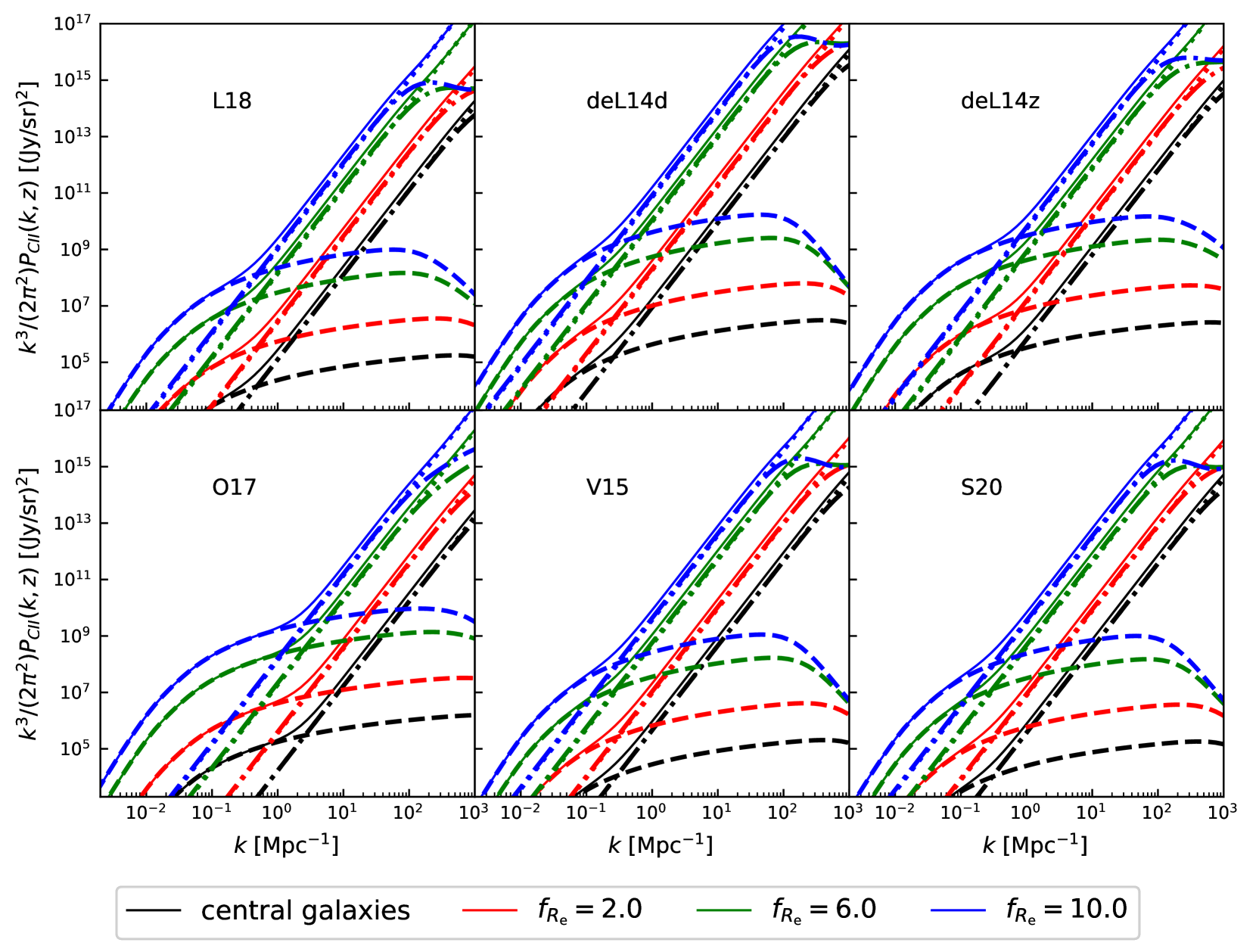
Figure 3: Predicted [C $\scriptstyle\rm II$] power spectrum for six [C $\scriptstyle\rm II$] -SFR relations. The dash-dotted line, dashed line, dotted line, and thin solid line denote the one-halo, two-halo, shot noise terms, and the sum of them respectively, in both panels. The dotted line (shot noise) overlaps with the dash-dotted line (one-halo term) at a large scale. The black line represents the [C $\scriptstyle\rm II$] power spectrum for the central galaxy, i.e. without [C $\scriptstyle\rm II$] halo considered. Red, green, and blue lines corresponding to $f_{R_{\rm e}}=[2.0,6.0,10.0]$, with fixed $f_{\Sigma}\sim 0.4$.

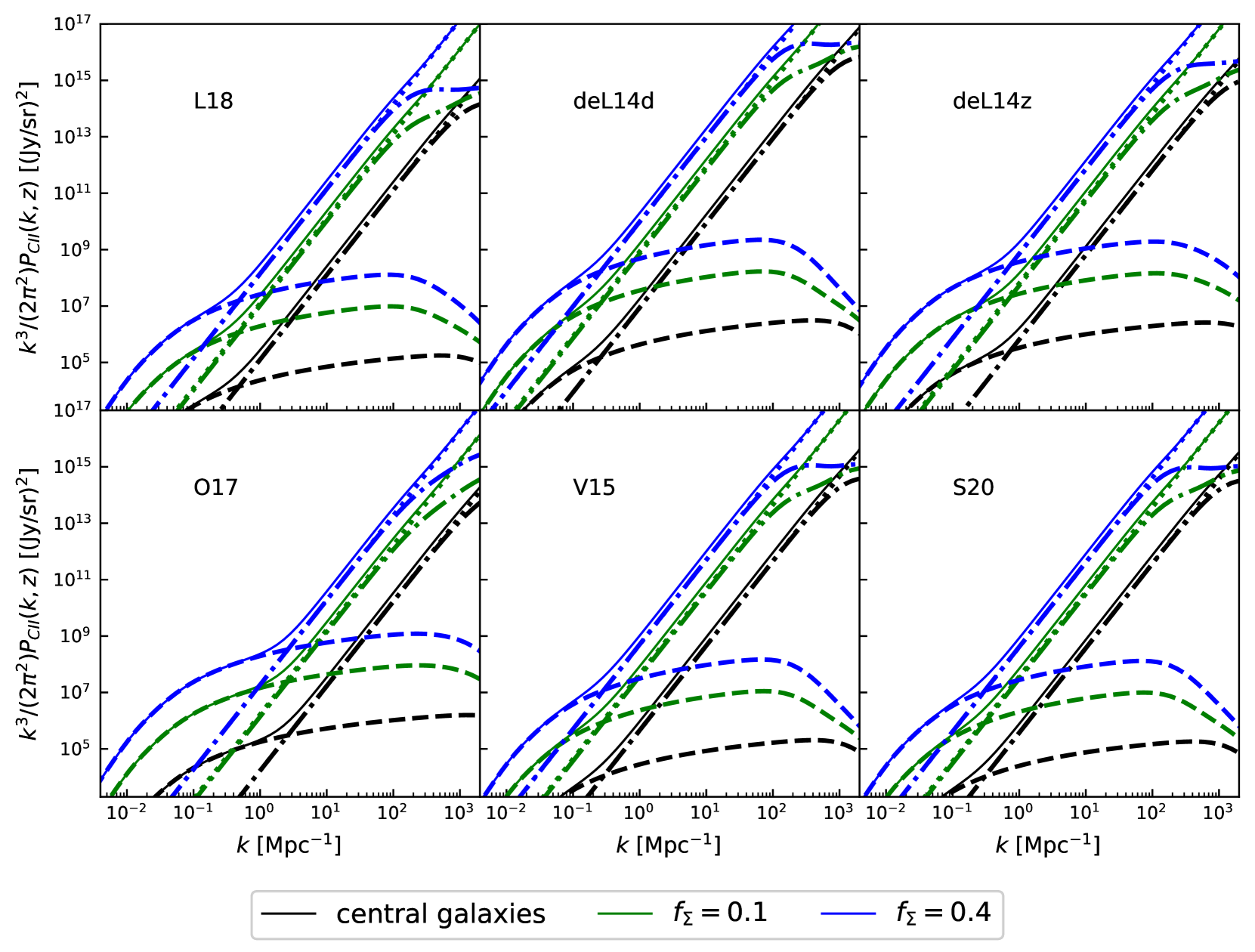
Figure 4: As in Fig. 3 for different values of $f_{\Sigma}$ and for the six different [C $\scriptstyle\rm II$] -SFR relations considered (see Tab. 1); we fix $f_{R_{\rm e}}=6.0$ here.

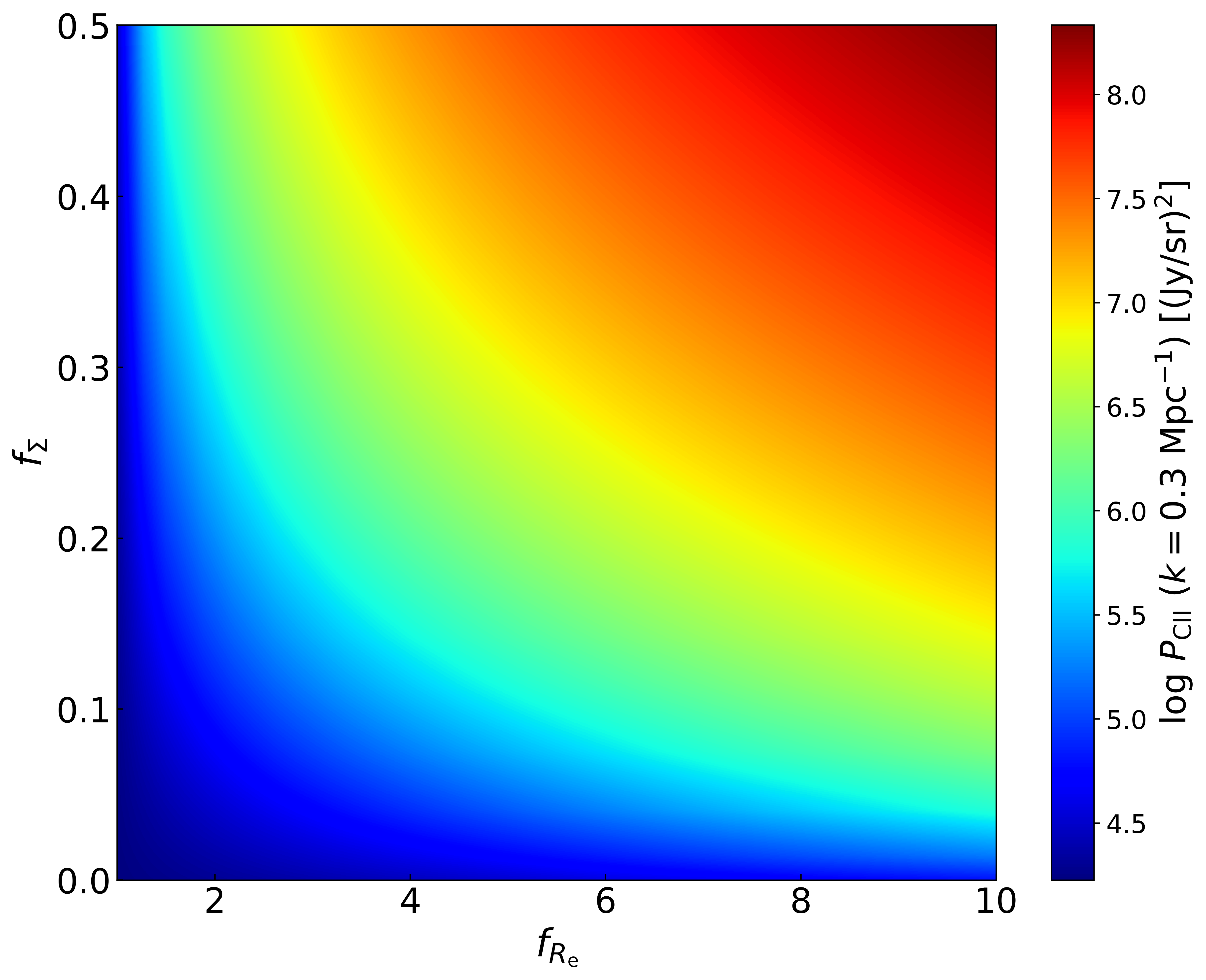
Figure 5: The total [C $\scriptstyle\rm II$] halo power spectrum at $k=0.3\ {\rm Mpc}^{-1}$ as a function of $f_{\Sigma}$ and $f_{R_{\rm e}}$, to avoid repetition we only show the result for L18 [C $\scriptstyle\rm II$] -SFR relation.

3.2 Detectability of the [C $\scriptstyle\rm II$] halo signal

We now turn the discussion to the detectability of the predicted [C $\scriptstyle\rm II$] power spectrum signal in a LIM survey.

3.2.1 Detectability in ALMA ASPECS Survey

The ALMA Large Program ASPECS (Aravena et al., 2020) surveying the Hubble Ultra Deep Field (HUDF) provides the first full frequency scan in Band 6, corresponding to the frequency window for [C $\scriptstyle\rm II$] emission from $6<z<8$ galaxies, we first consider the detectability of [C $\scriptstyle\rm II$] power spectrum signal by such an experiment.

The ASPECS Band 6 data covers a total area of $4.2\ \rm arcmin^{2}$ in the HUDF, with $2.9\ \rm arcmin^{2}$ area within the 50% primary beam response (Decarli et al., 2020). The observed frequency range is $212-272\ \rm GHz$, corresponding to the redshift range $z=5.99-7.97$ for the [C $\scriptstyle\rm II$] line. If we rebin the frequency channels by a factor of 8, as suggested by Uzgil et al. (2021), the spectral resolution is $\delta\nu_{0}=62.5\,\rm MHz$. The synthesized beam size (the FWHMs of the pixel ellipse along its major and minor axes, see Uzgil et al. 2019) in the image cube is $\Delta\theta_{\rm b,maj}\times\Delta\theta_{\rm b,min}=1.6^{\prime\prime}\times 1.1^{\prime\prime}$ (Uzgil et al., 2021). Then

$$\Omega_{\rm beam}=\frac{\theta_{\rm b,maj}\times\theta_{\rm b,min}}{2\ln 2}.$$ (51)

From these survey parameters, we derive $k_{\parallel,\rm min}=0.009\,\rm Mpc^{-1}$, $k_{\parallel,\rm max}=4.551\,\rm Mpc^{-1}$, $k_{\perp,\rm min}=1.503\,\rm Mpc^{-1}$, and $k_{\perp,\rm max}=68.147\,\rm Mpc^{-1}$, and we finally have $k_{\rm min}=1.503\,\rm Mpc^{-1}$, $k_{\rm max}=68.299\,\rm Mpc^{-1}$. We summarize the ASPECS survey parameters derived for the [C $\scriptstyle\rm II$] power spectrum analysis in Tab. 2.

Next, we compute the S/N of the [C $\scriptstyle\rm II$] power spectrum for an ASPECS-like survey. The survey has noise flux $\sigma_{\rm N}=0.30\,\rm mJy\,\rm beam^{-1}$ (Uzgil et al., 2021), which yields a surface brightness intensity sensitivity $\sigma_{\rm N}/\Omega_{\rm beam}=1.01\times 10^{7}\,\rm Jy\ sr^{-1}$, and a noise power spectrum $P_{\rm N}=1.48\times 10^{11}\ \rm(Jr/sr)^{2}\ \,{{\rm Mpc}}^{3}$ using Eq. (46).

We show the results of S/N for various $L_{\rm CII,SFR}-{\rm SFR}$ relations with $f_{\Sigma}=0.4$, $f_{R_{\rm e}}=2.0$ (left panel, represents a relatively compact [C $\scriptstyle\rm II$] halo) and $f_{\Sigma}=0.1$, $f_{R_{\rm e}}=6.0$ (right panel, represents a relatively diffuse [C $\scriptstyle\rm II$] halo) respectively in Fig. 6. In the left panel, only the signal of the deL14d [C $\scriptstyle\rm II$] - SFR model is detectable (with ${\rm S/N}\gtrsim 3$) in the range $10\,\rm Mpc^{-1}\lesssim k\lesssim 70\,\rm Mpc^{-1}$. In the right panel, the model deL14d is detectable in $4\,\rm Mpc^{-1}\lesssim k\lesssim 70\,\rm Mpc^{-1}$, while the model deL14$z$ is detectable in $10\,\rm Mpc^{-1}\lesssim k\lesssim 70\,\rm Mpc^{-1}$. This is because although the surface brightness of the [C $\scriptstyle\rm II$] halo is lower in the right panel, the total luminosity is larger as it scales with $f_{R_{\rm e}}^{2}$. We additionally demonstrate the impact of the shot noise on S/N by dotted lines. When shot noise is excluded, the resulting S/N is reduced by a factor of $\sim 2$. This is because the ASPECS has a small area. The detected power spectrum is basically the one-halo clustering term plus the shot noise, the two-halo clustering term is almost negligible. While the shot noise is comparable to the one-halo clustering term, excluding it will reduce the shot noise by a factor $\sim 2$.

Table 2: The ASPECS survey parameters for S/N analysis.

[$\nu_{0}-\Delta\nu_{0},\nu_{0}$]	[212—272] GHz
$z$	[5.99, 7.97]
$\delta\nu_{0}$	62.5 MHz
$\Omega_{\rm survey}$	$2.9\,\rm arcmin^{2}$
$\Omega_{\rm beam}$	$1.6^{\prime\prime}\times 1.1^{\prime\prime}$
$\sigma_{\rm N}$	0.30 mJy beam-1
$V_{\rm survey}$	13260 Mpc3
$\Delta r_{\parallel,\rm min}$	0.690 Mpc
$\Delta r_{\parallel,\rm max}$	662.701 Mpc
$\Delta r_{\perp,\rm min}$	0.046 Mpc
$\Delta r_{\perp,\rm max}$	4.180 Mpc
$k_{\parallel,\rm min}$	0.009 Mpc-1
$k_{\parallel,\rm max}$	4.551 Mpc-1
$k_{\perp,\rm min}$	1.503 Mpc-1
$k_{\perp,\rm max}$	68.299 Mpc-1
$k_{\rm min}$	1.503 Mpc-1
$k_{\rm max}$	68.299 Mpc-1
$P_{\rm N}$	$1.48\times 10^{11}$ (Jy/sr)2 Mpc3

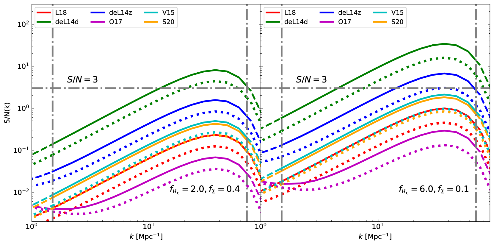
Figure 6: S/N for six different $L_{\rm CII,SFR}-\rm SFR$ relations for the ALMA ASPECS Survey. The solid lines represent the S/N for the total power spectrum (including contributions from one-halo and two-halo terms as well as shot noise), while the dotted lines illustrate the S/N when the shot noise is excluded. The $k_{\rm min}$ and $k_{\rm max}$ are shown as grey dashed-dotted vertical lines. Left panel: case with $f_{R_{\rm e}}=2.0,f_{\Sigma}=0.4$. Right panel: same for $f_{R_{\rm e}}=6.0,f_{\Sigma}=0.1$.

3.2.2 Optimal survey strategy

To optimally probe the extended [C $\scriptstyle\rm II$] halo signal, an ideal survey should be able to detect the signal with a resolution up to scale comparable to the extended [C $\scriptstyle\rm II$] halo size. On the other hand, to enhance the statistical significance of the signal, the survey should cover a sky area much larger than the ASPECS. Here we propose, by using ALMA 12-m antennas in an extended configuration with $\sim 1000$ m baseline, $N_{\rm an}=500$, and $N_{\rm chn}=1000$, to survey a total area of $\Omega_{\rm survey}\sim 2\,\rm deg^{2}$ in frequency band [212-272] GHz with total observing time $t_{\rm obs}\sim 1000\,\rm hr$. The frequency resolution $\delta\nu_{0}=\Delta\nu_{0}/N_{\rm chn}=60$ MHz.

The system temperature of ALMA at observing frequency $\nu_{0}=272\,\rm GHz$ is $T_{\rm sys}\sim 115\,\rm K$. Following the procedures in Section 2.4, we calculate the S/N and show them in Fig. 7. A summary of the parameters for this designed survey is given in Tab. 3.

For this optimized survey, when $f_{\Sigma}=0.4$ and $f_{R_{\rm e}}=2.0$ (see the left panel of Fig. 7), the [C $\scriptstyle\rm II$] power spectra of the six $L_{\rm CII,SFR}-\rm SFR$ relations all detectable with total signal-to-noise ratio $\gtrsim 10$. For the more extended [C $\scriptstyle\rm II$] halo model with $f_{\Sigma}=0.1$ and $f_{R_{\rm e}}=6.0$ (see the right panel of Fig. 7), the total signal-to-noise ratios of the power spectral are even higher. Similar to Fig. 6, we show the S/N if the shot noise is not involved by dotted lines. Different from the Fig. 6, when shot noise is excluded, the S/N does not change at $k\lesssim 0.1$ Mpc^-1. However, at $k\gtrsim 0.1$ Mpc^-1 where the shot noise dominates over the clustering term, the S/N is reduced by a factor $\sim 2$, similar to Fig. 6. This is natural since at $k\gtrsim 0.1$ Mpc^-1, the shot noise term is comparable to the one-halo clustering term.

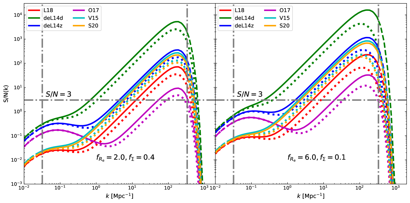
Figure 7: As in Fig. 6 but for the optimal survey strategy by using ALMA. With $1000\,\rm m$ baseline, the largest $k$ mode can be probed is $k_{\rm max}=331.43\,{\rm Mpc}^{-1}$. The signal for the six $L_{\rm CII,SFR}-\rm SFR$ relations can be detected by this configuration in both two cases.

Table 3: Parameters of a designed optimal survey

$d$	12 m
$T_{\rm sys}$	115 K
$N_{\rm an}$	500
$N_{\rm chn}$	1000
$b_{\rm max}$	1000 m
$\theta_{\rm beam}$	0.232′′
$[\nu_{0}-\Delta\nu_{0},\nu_{0}]$	[212,272] GHz
Redshift range	[6.0-8.0]
$\delta\nu_{0}$	60 MHz
$t_{\rm obs}$	1000 hr
$\Omega_{\rm survey}$	2 $\rm deg^{2}$
$V_{\rm survey}$	$2.88\times 10^{7}$ $\rm Mpc^{3}$
$V_{\rm vox}$	$5.96\times 10^{-5}$ $\rm Mpc^{3}$
$P_{\rm N}$	$4.87\times 10^{11}$ $\rm(Jy\ sr^{-1})^{2}\ Mpc^{3}$
$k_{\rm min}$	0.032 $\rm Mpc^{-1}$
$k_{\rm max}$	331.43 $\rm Mpc^{-1}$

3.3 Constraining the [C $\scriptstyle\rm II$]  halo parameters

We have shown that when the contribution from extended [C $\scriptstyle\rm II$] halos is considered, the [C $\scriptstyle\rm II$] power spectrum is boosted. However, this is mainly because the total [C $\scriptstyle\rm II$] luminosity of the system (central galaxy + [C $\scriptstyle\rm II$] halo) is larger. So there is a degeneracy between the [C $\scriptstyle\rm II$] halo contribution and the [C $\scriptstyle\rm II$] - SFR relation. [C $\scriptstyle\rm II$] halos also change the shape of the [C $\scriptstyle\rm II$] power spectrum (one-halo term) at scales comparable to their size. However, the scales are so small, that generally, the shot noise is much larger than the one-halo term. Here we investigate whether our designed optimal survey is able to put some conclusive constraints on the [C $\scriptstyle\rm II$] halo properties.

We first generate the mock observed power spectrum $P_{\rm CII}^{\rm obs}$ for our designed optimal survey from Eq. (26), by adopting $\log A=6.5$, $\gamma=1.2$, $f_{\Sigma}=0.1$ and $f_{R_{\rm e}}=6.0$ as the input [C $\scriptstyle\rm II$] halo parameters. Since in this paper we focus on constraining the [C $\scriptstyle\rm II$] halo parameters, we fix the cosmological parameters to reduce the freedoms. We adopt the cosmological parameters Planck Collaboration et al. 2016. The mock uncertainties are from Eq. (40). We then obtain the forecast on constraining the [C $\scriptstyle\rm II$] halo parameters by minimizing

$$\chi^{2}(\Theta)=\sum_{i=1}^{N_{\rm bin}}\frac{\left[P_{\rm CII}(k_{i},\Theta)-P_{\rm CII}^{\rm obs}(k_{i})\right]^{2}}{\sigma_{P}^{2}(k_{i})}$$ (52)

using the MCMC procedure (Goodman & Weare, 2010), where $\Theta=\{\log A,\gamma,f_{\Sigma},f_{R_{\rm e}}\}$ represents the $L_{\rm CII,SFR}-{\rm SFR}$ relation and extended [C $\scriptstyle\rm II$] halo parameters; $N_{\rm bin}$ is the number of $k$ bins between $k_{\rm min}$ and $k_{\rm max}$, with width $d\ln k=0.2$. When performing the MCMC procedure, we set flat priors $\log A\in[5.0,9.0],\gamma\in[0.1,2.0],f_{\Sigma}\in[0.0,0.5],f_{R_{\rm e}}\in[1.0,10.0]$.

In Fig. 8, we show the mock observed power spectrum with uncertainties and the best-fitting cure obtained from our MCMC fitting. The forecast on the constraints of [C $\scriptstyle\rm II$] halo parameters for our designed optimal survey is shown in Fig. 9. The marginalized parameters for [C $\scriptstyle\rm II$] halo are: $f_{\Sigma}=0.102^{+0.015}_{-0.018}$, $f_{R_{\rm e}}=5.894^{+0.912}_{-0.693}$. Indeed, it is feasible to distinguish the extended [C $\scriptstyle\rm II$] halo contribution to the power spectrum in this designed optimal survey. However, we also check that the ASPECS survey is still hard to give conclusive constraints, because of the smaller S/N and lower resolution.

We also perform a MCMC fitting for which we set the shot noise as an independent free parameter, instead of a function of $\Theta$. We obtain $f_{\Sigma}=0.216^{+0.152}_{-0.109}$ and $f_{R_{\rm e}}=5.917_{-0.686}^{+0.683}$. The constraints become looser. This is not surprising, because treating the shot noise as an independent parameter increases the degree of freedom. Moreover, in our case, the one-halo term contributes most to the constraints on [C $\scriptstyle\rm II$] halo parameters because it contains the information of [C $\scriptstyle\rm II$] luminosity profile. However, the shot noise, if expressed as a function of $\Theta$, also provides some constraints on $\Theta$. Shot noise is also a kind of useful signal, although using this term solely will suffer from heavy parameter degeneracy.

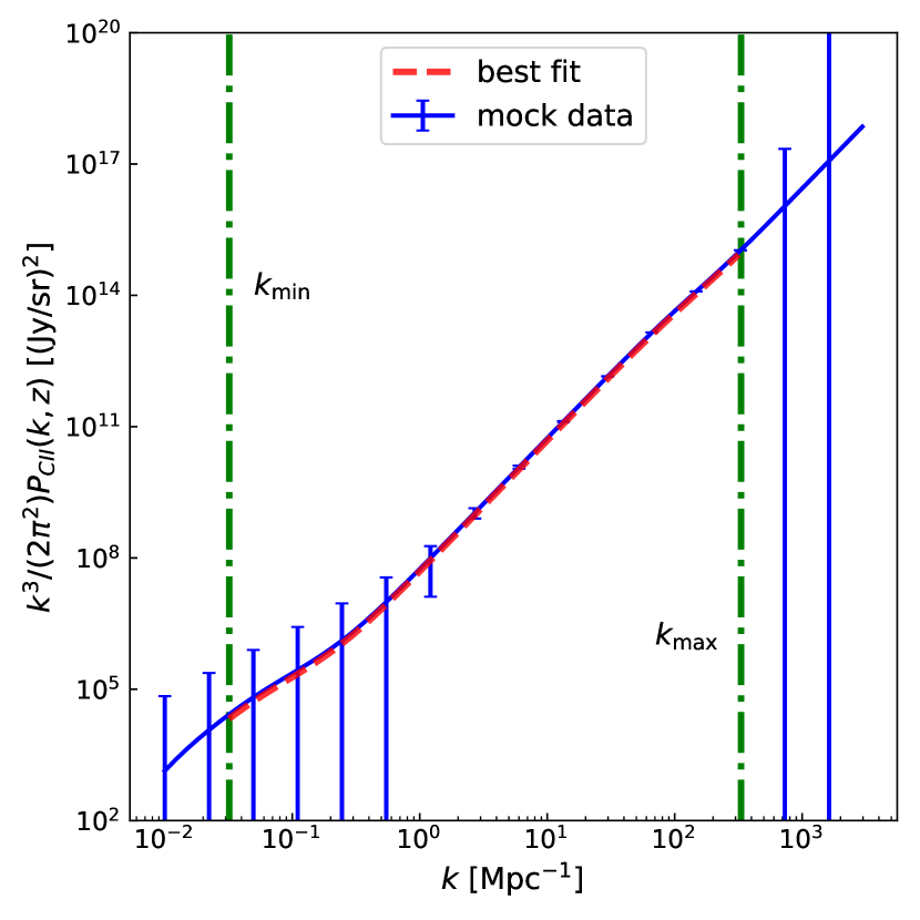
Figure 8: The mock observed power spectrum $P_{\rm CII}^{\rm obs}(k)$ (solid line with errorbars) and the best fitting power spectrum in $k_{\rm min}<k<k_{\rm max}$ (dashed line). We mark $k_{\rm min}$ and $k_{\rm max}$ by two vertical dashed-dotted lines.

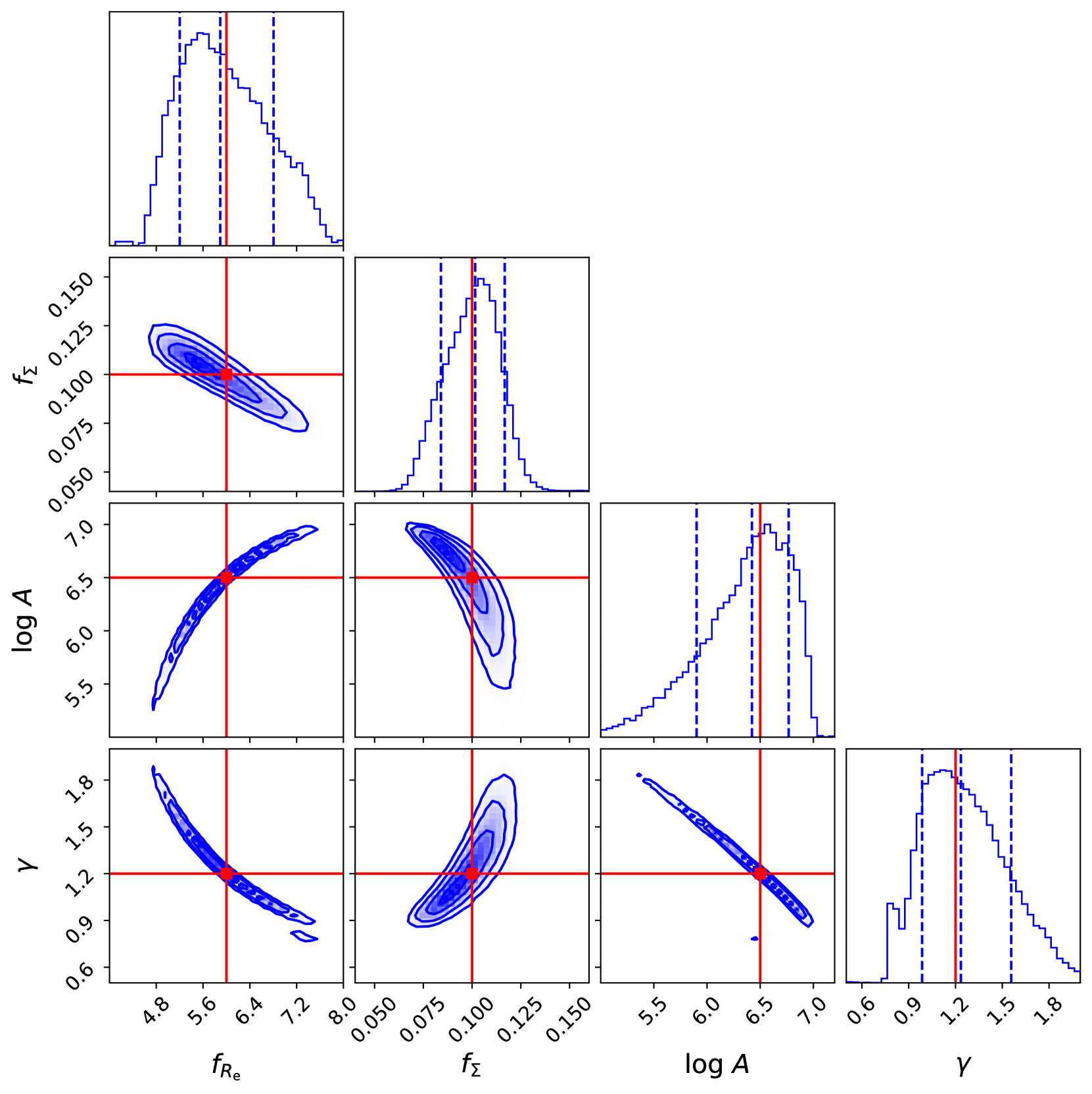
Figure 9: The forecast of confidence levels of the $L_{\rm CII,SFR}-{\rm SFR}$ relation and [C $\scriptstyle\rm II$] halo parameters obtained by the optimized survey. We mark the input parameters by the crosses of vertical and horizontal lines.

4 Conclusions

In this paper, we predicted the foreground- and contamination-cleaned [C $\scriptstyle\rm II$] power spectrum signal at $z\approx 6$, when both central galaxies and extended [C $\scriptstyle\rm II$] halos are considered, and investigate the detectability of such signal using ALMA ASPECS survey and a designed optimized survey. We modelled the [C $\scriptstyle\rm II$] luminosity profiles of the central galaxy and extended [C $\scriptstyle\rm II$] halo by a $\rm S\acute{e}rsic$+exponential profile, and derive the [C $\scriptstyle\rm II$] - dark matter halo mass relation by matching the dark matter halo mass function with dust-corrected UV luminosity function of high-redshift galaxies. The main results are:

• The extended [C $\scriptstyle\rm II$] halos around high redshift galaxies can significantly enhance the LIM signal compared with the signal produced by central galaxies alone, both in terms of the clustering signal and shot noise.

• Our [C $\scriptstyle\rm II$] halo model has two free parameters: the effective [C $\scriptstyle\rm II$] halo/galaxy radius ratio, $f_{R_{\rm e}}$, and the central surface brightness ratio, $f_{\Sigma}$. The luminosity of extended [C $\scriptstyle\rm II$] halos is $\sim 2.24f_{\Sigma}f_{R_{\rm e}}^{2}$ times the central galaxies. When the [C $\scriptstyle\rm II$] halo contribution is included, compared with the power spectrum from central galaxies only, the signal is boosted by a factor from $\sim 20$ to $\sim 10^{3}$ when $f_{R_{\rm e}}$ varies between $2.0$ to $6.0$, if $f_{\Sigma}=0.4$. Given $f_{R_{\rm e}}=6.0$, the power spectrum is enhanced by $\sim 100$ to $\sim 10^{3}$ times when $f_{\Sigma}$ changes from 0.1 to 0.4.

• For a LIM experiment configured as the ALMA ASPECS Large Program (with resolution $\theta_{\rm beam}=1.13^{\prime\prime}$ and survey area $\Omega_{\rm survey}=2.9\,\rm arcmin^{2}$), the [C $\scriptstyle\rm II$] power spectrum signal is detectable (S/N$\gtrsim 3$) for the deL14d $L_{\rm CII,SFR}-{\rm SFR}$ relation with $f_{\Sigma}=0.4$ and $f_{R_{\rm e}}=2.0$, and for the deL14d, deL14$z$ relations with $f_{\Sigma}=0.1$ and $f_{R_{\rm e}}=6.0$. So for a LIM experiment, the signal of more extended, low surface brightness [C $\scriptstyle\rm II$] halos is more easily detected.

• To optimally detect the signal, we proposed an optimized survey using more ALMA antennas and longer baselines. The survey has a higher resolution ($\theta_{\rm beam}\sim 0.232^{\prime\prime}$) and larger survey area ($\Omega_{\rm survey}\sim 2\,\rm deg^{2}$). The resulting signal-to-noise ratio is large enough so that the signal from six $L_{\rm CII,SFR}-{\rm SFR}$ relations is detectable. We also predicted the confidence levels of the constraints on the $L_{\rm CII,SFR}-{\rm SFR}$ relation and [C $\scriptstyle\rm II$] halo parameters by this optimized survey. These two halo parameters are degenerate, but we still expect to obtain meaningful constraints, with uncertainties of $\sim 15\%$ on $f_{\Sigma}$ and $\sim 10\%$ on $f_{R_{\rm e}}$.

In this work, we ignored the continuum foreground and the interloping lines, assuming they could be ideally removed and a clean [C $\scriptstyle\rm II$] signal plus pure instrumental white noise is obtained. In practice, however, this is quite a challenge. The IR continuum foreground from dust emission of extragalactic star-forming galaxies can be $\gtrsim 10^{3}$ times higher than the [C $\scriptstyle\rm II$] LIM signal (e.g. Yue et al. 2015; Béthermin et al. 2022; Van Cuyck et al. 2023), while the interloping lines (for example the CO and [C$\scriptstyle\rm I$] lines from low redshift galaxies) can also be much higher than the [C $\scriptstyle\rm II$] line signal (e.g. Yue & Ferrara 2019; Béthermin et al. 2022; Van Cuyck et al. 2023). The Galactic dust emission and CMB also play a crucial role (Yue & Ferrara, 2019). In our model, the [C $\scriptstyle\rm II$] LIM signal is enhanced because of the contribution from [C $\scriptstyle\rm II$] halos. However, it is still far from enough to overcome the foreground/intervening lines. Many methods have been proposed to remove the foreground and interloping lines. We list some of them in Appendix B. We refer interested readers to the references therein.

To show the influence of foreground and interloping lines, one can make mock observations by simulations, and then apply the removal algorithms. However, it is beyond the scope of this work. Generally, if there are some residual foreground/interloping lines, particularly at a small scale, our constraints on the [C $\scriptstyle\rm II$] halo parameters will be biased.

Our predictions depend on the effective radius ratio, the central surface brightness ratio, and the choice of the $L_{\rm CII,SFR}-\rm SFR$ relation. Therefore, detection of the [C $\scriptstyle\rm II$] halo signal in the LIM power spectrum can be used to verify whether [C $\scriptstyle\rm II$] halos are ubiquitous in high-redshift galaxies, and provide information about [C $\scriptstyle\rm II$] halo size, and their possible relation with outflows carrying the emitting material out of the main galaxy body. Finally, it can be potentially used to constrain the $L_{\rm CII,SFR}-\rm SFR$ relation at high-$z$ as the amplitude of the power spectrum is sensitive to such quantity.

Data Availability

The data produced in this study are available from the corresponding author upon reasonable request.

Appendix A Profile deprojection

The deprojection of the 2D surface density profile $\Sigma(R)$ is the inversion of the Abel integral (Binney & Mamon, 1982; Binney & Tremaine, 1987)

$$\rho(r)=-\frac{1}{\pi}\int_{r}^{+\infty}\frac{d\Sigma}{dR}\frac{dR}{\sqrt{R^{2}-r^{2}}},$$ (53)

where $r$ is the 3D radius, $\rho(r)$ is the 3D density profile. For the $\rm S\acute{e}rsic$ model of $\Sigma(R)$, the exact analytical expression of the above integral involves the Meijer G special function (Mazure & Capelato, 2002; Baes & Gentile, 2011) or Fox H function (Baes & Gentile, 2011), both of them are complicated. Therefore, several analytical approximations are also proposed. They are described in detail in Vitral & Mamon (2020) and references therein. Here we choose to use the analytical approximation given by Prugniel & Simien (1997). In this model, one writes the dimensionless 3D density profile as

$$\tilde{\rho}(x)=\frac{b_{n}^{(3-p_{\rm n})n}}{n\Gamma[(3-p_{\rm n})n]}x^{-p_{\rm n}}\exp\left[-b_{\rm n}x^{1/n}\right]$$ (54)

where $x=r/R_{\rm e}$, $p_{\rm n}$ is a function depending on the index $n$,

$$p_{\rm n}=1-\frac{0.594}{n}+\frac{0.055}{n^{2}}.$$ (55)

Therefore, in our model, the 3D luminosity density profile for the central galaxies can be written as

$$\rho_{\rm CII,g}(r) =\frac{L_{\rm CII,g}}{4\pi R_{\rm e,g}^{3}}\tilde{\rho}(x)$$ (56)

$$=\frac{L_{\rm CII,SFR}}{4\pi R_{\rm e,g}^{3}}\frac{(b_{n})^{(3-p_{\rm n})n}}{n\Gamma[(3-p_{\rm n})n]}x^{-p_{\rm n}}\exp\left[-b_{n}x^{1/n}\right].$$

For the extended [C $\scriptstyle\rm II$] halo, since the exponential profile corresponds to the $\rm S\acute{e}rsic$ model with $n=1$, one can easily derive $\rho_{\rm CII,h}(r)$ by analogizing to Eq. (56) and replacing $L_{\rm CII,g}$ with $L_{\rm CII,h}$,

$$\rho_{\rm CII,h}(r) =\frac{L_{\rm CII,h}}{4\pi R_{\rm e,h}^{3}}\frac{(b_{1})^{(3-p_{\rm 1})}}{\Gamma[(3-p_{\rm 1})]}x^{-p_{\rm 1}}\exp\left[-b_{1}x\right]$$ (57)

$$=\frac{L_{\rm CII,SFR}}{4\pi R_{\rm e,g}^{3}}\frac{f_{\Sigma}}{f_{R_{\rm e}}}\frac{1}{n}\frac{\Gamma(2)}{\Gamma(2n)}\frac{(b_{n})^{2n}(b_{1})^{(1-p_{\rm 1})}}{\Gamma[(3-p_{\rm 1})]}$$

$$\times x^{-p_{\rm 1}}\exp\left[-b_{1}x\right].$$

Appendix B Contamination removal

Here we briefly introduce some foreground/interloping line removal methods for LIM in literature.

By taking the advantage that the foreground is generally smooth in frequency space (Wang et al., 2006), the most popular way is to fit the IR continuum of each line of sight by a polynomial, then subtract it from the line of sight spectrum to get the residual LIM signal (Yue et al., 2015).

Moreover, one can also separate the smooth continuum foreground and the fluctuating LIM signal through the standard principal component analysis (PCA) (Yue et al., 2015; Bigot-Sazy et al., 2015; Van Cuyck et al., 2023) or the asymmetric re-weighted penalized least-squares (arPLS) method (Van Cuyck et al., 2023).

Recently, it has been demonstrated that deep learning has the potential to be a powerful tool for removing continuum foreground, interloping lines, and noise and finally reconstructing the 3D distribution of the target emission line (Moriwaki et al., 2020, 2021; Moriwaki & Yoshida, 2021; Makinen et al., 2021; Zhou et al., 2023).

If the LIM survey area overlaps with a galaxy survey, to migrate the foreground and interloping lines, one can also simply mask the voxels occupied by bright low redshift galaxies that are suspected contamination sources (Yue et al., 2015; Silva et al., 2015; Sun et al., 2018; Yue & Ferrara, 2019; Béthermin et al., 2022; Van Cuyck et al., 2023), or blindly mask a small fraction of bright voxels (Breysse et al., 2015).

For removing the interloping lines from low redshift galaxies, one can also take the advantage that their cylinder power spectrum is asymmetry if they are incorrectly identified as the target emission line (Lidz & Taylor, 2016; Cheng et al., 2016; Yue & Ferrara, 2019; Gong et al., 2020).

Breysse et al. (2016); Breysse et al. (2019) also proposed that the one-point statistics can migrate the continuum foreground and the interloping lines, and get the luminosity function of the target emission line.

Cheng et al. (2020) proposed that, if multiple lines of sources are observed at multiple frequencies, then the target signal can be extracted by fitting the observations to a set of spectrum templates.

Finally, the cross-correlation between [C $\scriptstyle\rm II$] line and the 21 cm line can be used to distinguish the signal and contaminations (Gong et al., 2011; Silva et al., 2015), while the cross-correlation between foreground lines and galaxy surveys are also explored in Silva et al. (2015) in order to probe the intensity of the foregrounds.

References

- Akins et al. (2022) Akins H. B., et al., 2022, ApJ, 934, 64
- Aravena et al. (2020) Aravena M., Carilli C., Decarli R., Walter F., ASPECS Collaboration 2020, The Messenger, 179, 17
- Baes & Gentile (2011) Baes M., Gentile G., 2011, A&A, 525, A136
- Bakx et al. (2020) Bakx T. J. L. C., et al., 2020, MNRAS, 493, 4294
- Baldauf et al. (2013) Baldauf T., Seljak U., Smith R. E., Hamaus N., Desjacques V., 2013, Phys. Rev. D, 88, 083507
- Battye et al. (2013) Battye R. A., Browne I. W. A., Dickinson C., Heron G., Maffei B., Pourtsidou A., 2013, MNRAS, 434, 1239
- Bernal & Kovetz (2022) Bernal J. L., Kovetz E. D., 2022, A&ARv, 30, 5
- Bernal et al. (2019) Bernal J. L., Breysse P. C., Gil-Marín H., Kovetz E. D., 2019, Phys. Rev. D, 100, 123522
- Béthermin et al. (2022) Béthermin M., et al., 2022, A&A, 667, A156
- Bigot-Sazy et al. (2015) Bigot-Sazy M. A., et al., 2015, MNRAS, 454, 3240
- Binney & Mamon (1982) Binney J., Mamon G. A., 1982, MNRAS, 200, 361
- Binney & Tremaine (1987) Binney J., Tremaine S., 1987, Galactic dynamics
- Bouwens et al. (2015) Bouwens R. J., et al., 2015, ApJ, 803, 34
- Breysse et al. (2014) Breysse P. C., Kovetz E. D., Kamionkowski M., 2014, MNRAS, 443, 3506
- Breysse et al. (2015) Breysse P. C., Kovetz E. D., Kamionkowski M., 2015, MNRAS, 452, 3408