Label Dependencies-aware Set Prediction Networks for Multi-label Text Classification

Abstract

Multi-label text classification aims to extract all the related labels from a sentence, which can be viewed as a sequence generation problem. However, the labels in training dataset are unordered. We propose to treat it as a direct set prediction problem and don’t need to consider the order of labels. Besides, in order to model the correlation between labels, the adjacency matrix is constructed through the statistical relations between labels and GCN is employed to learn the label information. Based on the learned label information, the set prediction networks can both utilize the sentence information and label information for multi-label text classification simultaneously. Furthermore, the Bhattacharyya distance is imposed on the output probability distributions of the set prediction networks to increase the recall ability. Experimental results on four multi-label datasets show the effectiveness of the proposed method and it outperforms previous method a substantial margin.

1 Introduction

Text classification is a crucial aspect of text mining, consisting of multi-class and multi-label classification. Traditional single-label text classification, it can offer more detailed and nuanced information, as well as a better reflection of the complexity and diversity of the real world by classifying a given document into different topics. Multi-label text classification aims to assign text data to multiple predefined categories, which may overlap. Thus, the overall semantics of the whole document can be formed by multiple components. In this paper, our focus is on multi-label text classification (MLTC), since it has become a core task in natural language processing, and has found extensive applications in various fields, including topic recognition[1], question answering[2], sentimental analysis[3], intent detection[4] and so on.

There are four types of methods for the MLC task[5]: problem transformation methods[6, 7], algorithm adaption methods[8], ensemble methods[9, 10] and neural network models[11, 12]. Till now, in the community of machine learning and natural language processing, researchers have paid tremendous efforts on developing MLTC methods in each facet. Among them, deep learning-based methods such as CNN[13][14], RNN[15],combination of CNN and RNN[16, 17], attention mechanism [1, 18, 19]and etc., have achieved great success in document representation. However, most of them only focus on document representation but ignore the correlation among labels. Recently, some methods including DXML[20], EXAM[21], SGM[5],GILE[22] are proposed to capture the label correlations by exploiting label structure or label content. Although they obtained promising results in some cases, they still cannot work well when there is no big difference between label texts (e.g., the categories Management vs Management moves in Reuters News), which makes them hard to distinguish.

However, taking the multi-label text classification as sequence to sequence problem, we should consider the order of the labels. Inspired by the set prediction networks for joint entity and relation extraction[23], we formulate the MLTC task as a set prediction problem and propose a novel Label Dependencies-aware Set Prediction Networks model(LD-SPN) for multi-label classification. In detail, there are three parts in the proposed method: set prediction networks for label generation, graph convolutional network to model label dependencies and Bhattacharyya distance module to make the output labels more diverse to elevate recall ability. The set prediction networks include encoder and decoder and the BERT model[24] is adopted as the encoder to represent the sentence, then we leverage the transformer-based non-autoregressive decoder[25] as the set generator to generate labels in parallel and speed up inference. Since such set prediction networks ignore the relevance of the labels, we model the label dependencies via a graph and use graph convolutional network to learn node representations by propagating information between neighboring nodes based on the adjacency matrix. Finally, the output distributions of the queries may overlap, which deteriorate the recall performance for label generation. In order to improve the recall ability of the model, we use the Bhattacharyya distance to calculate the distance between the output label distribution, making the distribution more diverse and uniform[26].

We summarize the main contributions as follows:

• We propose to view the multi-label text classification as a sequence to sequence generation problem and treat multi-label extraction through direct set prediction, the network featured by transformers with non-autoregressive parallel decoding is used to solve the set prediction problem.

• We design an adjacency matrix to model the label dependencies, which is constructed by mining the statistical relations between labels and a graph convolutional network (GCN) is employed to learn node representations by propagating information between neighboring nodes.

• We present a feature extraction method by utilizing an error estimation equation based on the Bhattacharyya distance between output distribution to improve the recall ability.

• Extensive experimental results show that our model consistently outperforms the strong baselines, and further experiments to demonstrate the effectiveness of the components of our model.

2 Related Work

2.1 Multi-label Classification

Compared with multi-class Classification, which assigns one label for each sample, several number of labels will be assigned in multi-label classification(MLC). Assume all the labels consist of $\mathcal{Y}=\{y_{1},y_{2},...,y_{m}\}$, the multi-class task studies the classification problem where each single instance is associated with a set of labels simultaneously. Assume $\mathcal{X}$ denotes the instance space, then multi-label task learns a function $f(.):\mathcal{X}\to 2^{\mathcal{Y}}$ from a multi-label training data $D=\{\textbf{x}_{i},Y_{i}\}_{i}^{N}$, where $N$ is the number of training sample and each $Y_{i}\subset\mathcal{Y}$. While for a multi-class task, the learned classification function is $f(.):\mathcal{X}\to\mathcal{Y}$ and training data $D=\{\textbf{x}_{i},y_{i}\}_{i}^{N}$ where each label $y_{i}$ satisfies $Y_{i}\in\mathcal{Y}$.

There are several methods are used for the MLTC task. Binary relevance(BR)[6] and Label Powerset(LP)[7] transform the MLTC task as a single label classification problem. SGM[5] takes multi-label classification as a sequence generation problem and considers the correlations between labels. Other methods like AGIF [27] adopt a joint model with Stack-Propagation[28] to capture the intent semantic knowledge and perform the token level intent detection for multi-label classification. Our work is in line with sequence to sequence based methods and treat multi-label classification as a set prediction problem.

2.2 Set Prediction Networks

Set prediction networks are used to solve the seq2seq problem when to avoid considering the order of the generation process and it is employed to extract entity and relation[23]. The architecture of the set prediction networks are featured by transformers with non-autoregressive parallel decoding[29] bipartite matching loss. In detail, there are three parts in set prediction networks: a sentence encoder, a set generator, and a set based loss function. Traditional neural networks such as LSTM[30] or pretraining language model BERT[24] are usually severed as the encoder. Since an autoregressive decoder is not suitable for generating unordered sets, the transformer-based non-autoregressive decoder[29] is acted as the set generator. In order to assign a predicted label to a unique ground truth label, bipartite matching loss function inspired by the assigning problem in operation research[31] is proposed. Apart from information extraction, set prediction networks are applied to object detection[32, 33].

3 Proposed Method

In this section, we will present the overview of our proposed method and is demonstrated in Figure 1. It consists of three parts: set prediction networks, GCN module, Bhattacharyya distance module. The set prediction networks predict the multi-labels simultaneously by combining a BERT encoder for sentence representation and the label dependencies learned by GCN with a non-augoregressive decoder. Bhattacharyya distance is imposed on the output distribution of the set prediction networks and bipartite matching loss between the ground truths and predictions is optimized to obtain the predicted labels. Each module of the framework will be detailed in the following.

3.1 Overview

The goal of multi-label classification is to identify all possible label from a given sentence and similar to[34], we take it as a sequence to sequence problem. Formally, given a sentence $X$, the conditional probability of the corresponding multi-label set $Y=\{y_{1},y_{2},...,y_{n}\}$ is formulated as:

$$P(Y|X,\theta)=\prod_{i=1}^{n}p(y_{i}|X,y_{j<i};\theta)$$ (1)

the autoregressive factorization predicted the labels in sequential which prevents architectures like the Transformer from fully realizing their training-time performance advantage during inference. Non-autoregressive decoding [29] is proposed to remove the autoregressive connection from the existing encoder-decoder model. Assuming the number of the predicted labels $n$ can be modeled with a separated conditional distribution $p_{N}$, then the conditional probability distribution for multi-label classification using non-autoregressive becomes:

$$P(Y|X,\theta)=p_{N}(n|X;\theta)\prod_{i=1}^{n}p(y_{i}|X;\theta)$$ (2)

In the following, similar to the non-autoregressive loss function used for triple extraction in[23], the conditional probability $p(Y_{i}|X;\theta)$ in (2) is parameterized by a non-autoregressive transformer network and the multi-label classification is viewed as a direct set prediction problem.

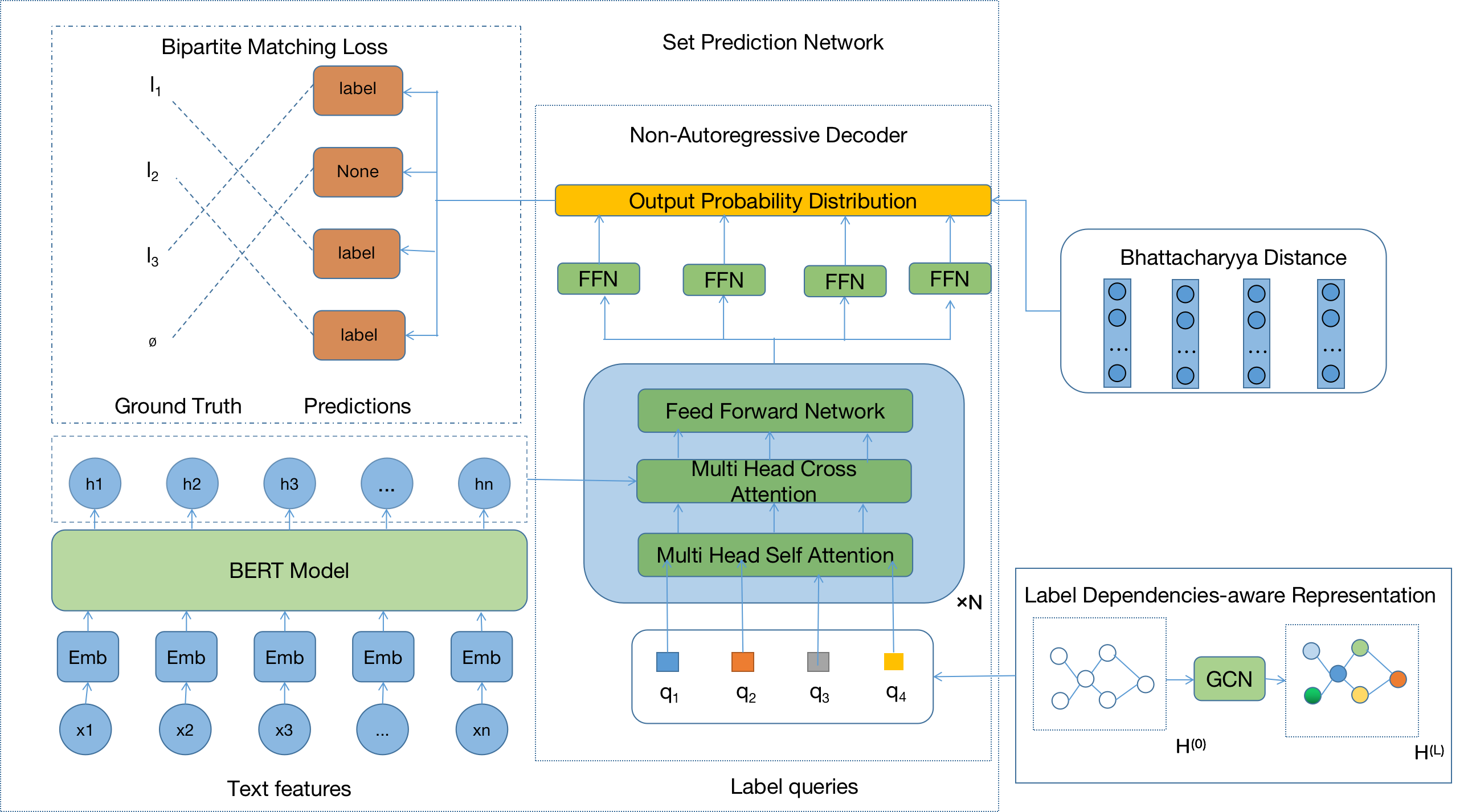
Figure 1: Overall architecture of our LD-SPN model. The set prediction networks predict the multi-labels simultaneously by combining a BERT encoder for sentence representation and the label dependencies learned by GCN with a non-augoregressive decoder. Bhattacharyya distance is imposed on the output distribution of the set prediction networks and bipartite matching loss between the ground truth and predictions is optimized to obtain the predicted labels.

3.2 Multi-Label Generation

Sentence Encoder

BERT has achieved impressive performance in many natural language processing task, it is used as our sentence encoder. The input sentence is segmented with tokens and each sentence is represented through its token ids, token type ids and attention mask. Then through a multi-layer Transformer[35] block, the output of the BERT model is the context aware embedding of tokens and denoted as $\textbf{H}\in\mathbf{R}^{l\times d}$. where $l$ is the length of the sentence with two special token [CLS] and [SEP], $d$ is the dimension of the output of the last hidden states.

Non-Autoregressive Decoder

In multi-label classification, each instance may have different number of labels. Instead of computing the probability $p_{N}(n|X)$ of the number of labels for each sentence $X$, we treat it as a fixed constant number $m$ which is larger than the typical number of labels in sentences appeared in the training data.

We regard the multi-label classification as a set prediction problem and the decoder process follows as the standard architecture of the transformer. In order to predict the $m$ labels simultaneously, the input embeddings for the decoder are the $m$ learned label embeddings which is referred as label queries and the embeddings of the sentence through the pre-trained language model BERT. In order to make the query label embeddings independent, they are usually initialized with an orthogonal matrix.

Set Prediction Loss

Since the predicted labels are unordered and loss function should be invariant to any permutation of predictions, we adopt bipartite matching loss to measure the distance between the ground truths and predictions. Let $\mathbf{Y}=\{Y_{i}\}_{i=1}^{n}$ denote the set of ground truth labels and $\mathbf{\hat{Y}}=\{\hat{Y}_{i}\}_{i=1}^{m}$ the set of predicated labels for one sample, where $m$ is larger than $n$. Here we extend the number of each ground truth label to $m$ labels which padded with the empty label type $\emptyset$. Each $Y_{i}=(l_{t})$ is the index of the label and $l_{t}$ can be $\emptyset$, $t\in\{1,2,...,m\}$. Each element of the predicted labels $\hat{Y}_{i}=\{\mathbf{p}_{i}^{l}\}$, which is computed via softmax function.

To compute the bipartite matching loss, we should first solve the optimal matching between the ground truth labels $\mathbf{Y}$ and the predicted labels $\mathbf{\hat{Y}}$. The matching solution can be derived from the following optimization:

$$\pi^{*}=\arg min_{\pi\in\Pi(m)}\sum_{i=1}^{m}\mathcal{C}_{match}(Y_{i},\hat{Y}_{\pi(i)})$$ (3)

where $\Pi(m)$ is the space of all $m$-length permutations. Each element in the summation of the equation is defined as:

$$\mathcal{C}_{match}(Y_{i},\hat{Y}_{j})=-I_{\{l_{i}\neq\emptyset\}}[\mathbf{p}_{j}^{l}(l_{i})]$$ (4)

After getting the optimal correspondence $\pi^{*}$ between the ground truth labels and the predicted labels, the bipartite matching loss is computed as follows:

$$\mathcal{L}(\mathbf{Y},\mathbf{\hat{Y}})=\sum_{i=1}^{m}-\log\mathbf{p}_{\pi^{*}(i)}^{l}(l_{i})$$ (5)

3.3 Label Dependencies-aware Representation

For the naive set prediction networks used for multi-label text classification, the queries used to generate the predicted labels don’t consider the dependencies of the labels, which are usually initialized as random orthogonal matrix. Since labels are correlated, we model the label dependency via a graph, which is effective in capturing the relationship among labels[36] and GCN is employed to learn the label dependencies. First, we count the number of occurance of label pairs in the training data and get a matrix $C\in R^{K\times K}$, where $K$ is the number of distinct labels in the training set, $C_{ij}$ denotes the co-occurance times of the label $l_{i}$ and $l_{j}$. Then a conditional probability matrix $P\in R^{K\times K}$ is obtained through:

$$P_{ij}=X_{ij}/X_{i.}$$ (6)

where $P_{ij}$ denotes the conditional probability of label $l_{j}$ occurs when label $l_{i}$ appears, $X_{i.}$ denotes the occurrence times of label $l_{i}$ in the training set.

In order to avoid the over-fitting of the training data[37], a threshold $\tau$ is utilized to truncate the small conditional probability and we get a weighted adjacency matrix $A$.

$$A_{ij}=\left\{\begin{aligned} 0\quad P_{ij}<\tau\\ P_{ij}\quad P_{ij}\geq\tau\\ \end{aligned}\right.$$ (7)

Since many 0s maybe appear in adjacency matrix $A$, which cause over-smoothing, i.e. the node features maybe indistinguishable from different clusters as the GCN layer deepens[38]. Therefore, we adopt an re-weighted schema for adjacency matrix as[39] for node information propagation in GCN.

$$A_{ij}^{{}^{\prime}}=\left\{\begin{aligned} pA_{ij}/\sum_{i=1,i\neq j}^{N}A_{ij}\quad i\neq j\\ 1-p\quad i=j\\ \end{aligned}\right.$$ (8)

where the parameter $p$ determine the weight assigned to itself and its neighbor. When $p$ approaches 1, the information of the node itself will not considered, as $p$ tends to 0, the information of its neighbor will be weakened.

Given the adjacency matrix $A^{{}^{\prime}}$, each GCN layer takes the node information $H^{(l)}\in\mathbb{R}^{K\times c_{l}}$ in the $l-$th layer as inputs and outputs the node representation $H^{(l+1)}\in\mathbb{R}^{K\times c_{l+1}}$, where $c_{l}$ and $c_{l+1}$ denotes the dimension the node representation in the $l-$th and $(l+1)-$th layer respectively. The multi-layer GCN follows the layer-wise propagation rule between the nodes[39]:

$$H^{(l+1)}=h(\tilde{D}^{-\frac{1}{2}}\tilde{A}\tilde{D}^{-\frac{1}{2}}H^{(l)}W^{(l)})$$ (9)

Here $\tilde{D}^{-\frac{1}{2}}\tilde{A}\tilde{D}^{-\frac{1}{2}}$ is the normalized symmetric adjacency matrix, $\tilde{A}=A^{{}^{\prime}}+I_{K}$ is the adjacency matrix with self-connections, $I_{K}$ is the identity matrix. $\tilde{D}$ is a diagonal matrix with $\tilde{D}_{ii}=\sum_{j=1}^{N}\tilde{A}_{ij}$ in its diagonal, $W^{(l)}\in\mathbb{R}^{c_{l}\times c_{l+1}}$ is a training matrix in the $l-$th layer, $h(.)$ is an activation function in GCN.

According (9), each GCN layer takes the previous layer node representation $H^{(l)}$ as input and outputs $H^{(l+1)}$. The first layer node representation $H^{(0)}\in\mathbb{R}^{K\times c_{0}}$ is initialized as an orthogonal matrix. Assuming the number of layers of the GCN is $L$, the final node representation $H^{(L)}\in\mathbb{R}^{K\times c_{L}}$ is taken as the input as the query matrix in the set prediction networks for multi-label classification.

$$Q=W^{q}H^{(L)}$$ (10)

Here $W^{q}\in\mathbb{R}^{m\times K}$ transforms the labels representations from GCN to the input label queries embeddings for SPN, $m$ denotes the number of generated labels in set prediction networks.

3.4 Bhattacharyya Distance

The output distributions of the queries may overlap, which deteriorate the recall performance of set prediction networks. In order to make the output distribution more diverse, Bhattacharyya distance between the output distribution is imposed. Bhattacharyya distance measures the distance between two probability distributions[26],but it is not a metric since it does not obey the triangle inequality.

Suppose the $m$ output probability distribution are denoted as $\mathcal{P}=\{\textbf{p}_{1}^{l},\textbf{p}_{2}^{l},...,\textbf{p}_{m}^{l}\}$, the Bhattacharyya distance of this set of distribution is:

$$D_{B}(\mathcal{P})=\sum_{\textbf{p}^{l},\textbf{q}^{l}\in\mathcal{P}}-\log\sqrt{\sum_{i}\textbf{p}^{l}[i]\textbf{q}^{l}[i]}$$ (11)

Since the maximization of the Bhattacharyya distance results in the output probability distribution more dissimilar, while the optimization of the bipartite matching loss is minimization, we adopt minimize the Bhattacharyya coefficients to maximize the Bhattacharyya distance as follows:

$$BC(\mathcal{P})=\sum_{\textbf{p}^{l},\textbf{q}^{l}\in\mathcal{P}}\sqrt{\sum_{i}\textbf{p}^{l}[i]\textbf{q}^{l}[i]}$$ (12)

Finally, the loss function for LD-SPN is:

$$\mathcal{L}(Y,\hat{Y})=\sum_{i=1}^{m}-\log\mathbf{p}_{\pi^{*}(i)}^{l}(l_{i})+\lambda BC(\mathcal{P})$$ (13)

where $\lambda$ is a trade off between the diversity of output probability distribution (recall) and the precision of the set prediction networks for multi-label classification.

4 Experiments

In this section, four multi-label datasets will be used to evaluate our method . First we will give the description of each dataset, evaluation metrics, baseline methods and experimental settings. Then we compare the experimental results of our method with the baseline methods. Finally, we provide the analysis and discussions of experimental results.

4.1 Datasets

MixSNIPS: This dataset is collected from the Snips personal voice assistant[40] by using conjunctions, e.g., “and”, to connect sentences with different intents and ensure that the ratio of sentences has 1-3 intents is [0.3, 0.5, 0.2] [27]. Finally, they get the 45,000 utterances for training, 2,500 utterances for validation and 2500 utterances for testing on the MixSNIPS dataset.
MixATIS: This dataset is similar to MixSNIPS and created in [27], which is from the ATIS dataset [41]. There are 18,000 utterances for training, 1,000 utterances for validation and 1,000 utterances for testing.
Arxiv Academic Paper Dataset (AAPD): This dataset is collected from a English academic website in the computer science field. Each sample contains an abstract and the corresponding subjects. 54 labels are defined and 55,840 samples are included. which is used in [5] to test the performance of sequence generation model for multi-Label Classification. Reuters Corpus Volume I (RCV1-V2): This dataset is provided by [42]. It consists of over 800,000 manually categorized newswire stories made available by Reuters Ltd for research purposes. Multiple topics can be assigned to each newswire story and there are 103 topics in total.
Each datasets is split into train,valid and test dataset, the statistics of the datasets are show in Table 1.

Datasets	Train Samples	Valid Samples	Test Samples	Label Sets	W/S	L/S
MixSNIPS	45000	2500	2500	7	18.45	1.90
MixATIS	18000	1000	1000	18	20.23	1.90
AAPD	53840	1000	1000	54	163.42	2.41
RCV1-V2	775220	21510	7684	103	123.94	3.24

Table 1: Summary of dataset. Train Samples, Valid Samples, Test Samples and Label Sets denote the number of train, valid, test samples and labels, respectively. W/S is the number of words per sample and L/S is the number of labels per sample.

4.2 Evaluation Metrics

Following the previous work[5], we adopt hamming loss, micro-F1 score as our main evaluation metrics. besides, the micro-precision and micro-recall are also reported.

• Hamming-loss In multi-class classification, the Hamming loss corresponds to the Hamming distance between the ground true and predicted, which is equivalent to the subset zero-one loss function. In multi-label classification, the Hamming loss is different from the subset zero-one loss, it is more forgiving in that it penalizes only the individual labels and evaluates the fraction of misclassified instance-label pairs, where a relevant label is missed or an irrelevant is predicted[43].

• Micro-F1 It is a balance between the precision and recall and computed as a weighted average of the precision and recall[44]. It is calculated globally by counting the total true positives, false negatives, and false positives.

4.3 Baselines

Several multi-label classification methods are used to compare with our proposed model.
Binary Relevance(BR). [6] transforms the multi-label problem into several single label classification problems and ignore the correlation between labels.
Label Powerset(LP). [7] transforms the multi-label problem to a multi-class problem with one multi-class classifier trained on all unique label.
SGM. [5] takes multi-label classification as a sequence generation problem. To model the correlation between labels, a novel decode structure is used and a weighted global embedding based on all labels is computed as opposed to just the top one at each timestep.
AGIF. [27] adopts a joint model with Stack-Propagation[28] to capture the intent semantic knowledge and perform the token level intent detection to further alleviate the error propagation. In this paper, its variation is used to solve mult-label classification.
BERT-BCE. The pretraining language model BERT[24] is utilized to encode the input sentence and Binary Cross Entropy loss is employed to multi-label classification.

4.4 Experimental Settings

For text sequence encoding, we use the cased base version of BERT[24] in our experiments, which contains 110M parameters. The number of stacked bidirectional transformer blocks in non-autoregressive decoder is set to 2 for MixSNIPS and MixATIS dataset, 3 for AAPD and RCV1-V2 dataset. The threshold $\tau$ for the adjacency matrix in GCN is 0.1 and the smoothing parameter $p$ is set to 0.2, the hyperparameter $\lambda$ in (13) is chosen by grid search in $\{0.1,0.2,0.3,0.5,0.8\}$. The set prediction networks are trained by minimizing the loss function through stochastic gradient descent over shuffled mini batch with the AdamW update rule[45], the batch size is set to 16 for all datasets. All experiments are conducted with an NVIDIA A100 PCIE.

4.5 Main Results

Following SGM[5], we evaluate the performance of LD-SPN using F1 score and hamming-loss. We present the results of our implementations of our model as well as the baselines on four datasets on Table 2 and Table 3, respectively. Table 2 shows the experiment results of the proposed models on the MixATIS and MixSNIPS datasets. Table 3 shows the experiment results of the proposed models on the AAPD and RCV1-v2 datasets. Overall,our proposed model outperforms baselines on these datasets, BERT-BCE uses the pretrain language model to encode input sentence and get the second best performance. On the MixATIS dataset, the proposed LD-SPN model achieves $1.39\%$ improvement on F1 score and a reduction of 0.25% hamming-loss. On the MixSNIPS dataset,the proposed LD-SPN model achieves $0.5\%$ improvement on F1 score and a reduction of $0.28\%$ hamming-loss. On the AAPD dataset,the proposed LD-SPN model achieves $1.8\%$ improvement on F1 score and a reduction of $0.05\%$ hamming-loss. On the RCV1-v2 dataset,the proposed LD-SPN model achieves $2.9\%$ improvement on F1 score and a reduction of $0.22\%$ hamming-loss. We attribute this to the fact that our label dependency-aware set prediction networks can better help grasp the correlations between labels and improve overall contextual understanding, the Bhattacharyya distance imposed on output distribution to increase the recall ability.

Model	MixATIS
	F1(+)	P(+)	R(+)	HL(-)
BR	0.746	0.757	0.736	0.0537
LP	0.721	0.733	0.713	0.0648
SGM	0.84	0.844	0.837	0.0336
AGIF	0.767	0.813	0.754	0.0294
BERT-BCE	0.892	0.915	0.869	0.0223
LD-SPN	0.906	0.912	0.899	0.0198

(a) Performance on the MixATIS test set.

Model	MixSNIPS
	F1(+)	P(+)	R(+)	HL(-)
BR	0.843	0.855	0.831	0.0124
LP	0.815	0.813	0.817	0.0137
SGM	0.981	0.979	0.983	0.0098
AGIF	0.971	0.975	0.969	0.0152
BERT-BCE	0.978	0.978	0.979	0.0119
LD-SPN	0.983	0.984	0.982	0.0091

(b) Performance on the MixSNIPS test set.

Table 2: Comparison between our method and all baselines on MixATIS and MixSNIPS datasets. F1, P and R denote the F1 score, Precision and Recall, respectively. HL denotes the Hamming Loss,"-" means the smaller of the number the better, while "+" means the bigger of the number the better.

Model	AAPD
	F1(+)	P(+)	R(+)	HL(-)
BR	0.646	0.675	0.619	0.0316
LP	0.634	0.662	0.608	0.0343
SGM	0.710	0.748	0.675	0.0245
AGIF	0.683	0.726	0.644	0.0287
BERT-BCE	0.716	0.831	0.630	0.0224
LD-SPN	0.734	0.755	0.714	0.0229

(a) Performance on AAPD test set.

Model	RCV1-V2
	F1(+)	P(+)	R(+)	HL(-)
BR	0.415	0.364	0.483	0.0183
LP	0.503	0.481	0.526	0.0156
SGM	0.878	0.860	0.897	0.0075
AGIF	0.558	0.517	0.605	0.0107
BERT-BCE	0.862	0.825	0.903	0.0089
LD-SPN	0.891	0.871	0.912	0.0067

(b) Performance on RCV1-V2 test set.

Table 3: Comparison between our method and all baselines on AAPD and RCV1-V2 datasets. F1, P and R denote the F1 score, Precision and Recall, respectively. HL denotes the Hamming Loss,"-" means the smaller of the number the better, while "+" means the bigger of the number the better.

4.6 Ablation Study

In this section, we discuss how the classification loss function, label dependencies and the diversity of the query output probability distribution influence the performance. Besides, hyperparameters like the number of decoder layers in the non-autoregressive decoder, the number of query ]abels for decoding, the adjacency matrix smoothing thresholding parameter $\tau$ to model label dependencies, the coefficient $\lambda$ trade offs the precision and recall of the LD-SPN are taken into consideration. Since the the number of total labels for MixSNIPS and MixATIS datasets are relatively smaller than that of the AAPD and RCV1-V2 datasets, MixATIS and AAPD are chosen for different scene. Detailed results on these two dataset are shown in Table 4-7 and Figure 2, respectively.

Model	MixATIS
	F1(+)	P(+)	R(+)	HL(-)
BERT-BCE	0.892	0.915	0.869	0.0223
SPN	0.895	0.897	0.893	0.0218
LD-SPN	0.906	0.912	0.899	0.0198
wo/GCN	0.898	0.899	0.897	0.0215
wo/BC	0.902	0.909	0.895	0.0205

(a) Ablation study for LD-SPN on MixATIS test set.

Model	AAPD
	F1(+)	P(+)	R(+)	HL(-)
BERT-BCE	0.716	0.831	0.630	0.0234
SPN	0.724	0.784	0.673	0.0233
LD-SPN	0.734	0.755	0.714	0.0229
wo/GCN	0.726	0.745	0.707	0.0232
wo/BC	0.731	0.773	0.693	0.0231

(b) Ablation study for LD-SPN on AAPD test set.

Table 4: Ablation study on MixATIS and AAPD test set. SPN denotes the set prediction networks for multi-label classification while the query embedding is initialized as orthogonal matrix. wo/GCN denotes the LD-SPN model without GCN module for query embedding initialization. wo/BC denotes the LD-SPN without the module imposing Bhattacharyya distance for output distribution.

Exploration of the Classification Loss Function

Methods such as BERT-BCE and SPN both take the BERT model to encode the input sequence, while the former one use the Binary Cross Entropy loss for optimization, the second one take a number of query to decode the labels and utilize the Binary Matching Loss for optimization. From the first two rows in Table 4, we can see SPN obtain better results in F1 score and Hamming Loss, which show that compared to Binary Cross Entropy Loss, Binary Matching Loss may be a better choice for multi-label Classification.

Impact of the Label Dependencies-aware Representation

As show in the third row and fifth row from Table 4, through modeling the dependencies of labels, the proposed LD-SPN model shows better performance than the original SPN method for multi-label classification, and compared to the constraint imposed on the output distribution, the label dependencies have greater influence on the final performance of our proposed model.

Effectiveness of the Bhattacharyya Distance between Output Distribution

Comparing with the model without processing of the output distribution, the model with it show desired result in the recall performance. For MixATIS dataset, the recall performance is superior than the SPN model. while for the AAPD dataset,the recall of LD-SPN has increased about $3.0\%$ compared the model without it.

From Figure 2 we can see that the performance of LD-SPN on AAPD test set improves at first and then decrease as $\lambda$ increases, the best results have obtained when $\lambda$ equals to 0.2. Comparing with the SPN model just utilize the label dependencies, we find increasing the Bhattacharyya distance between Output Distribution can always achieve better recall score.

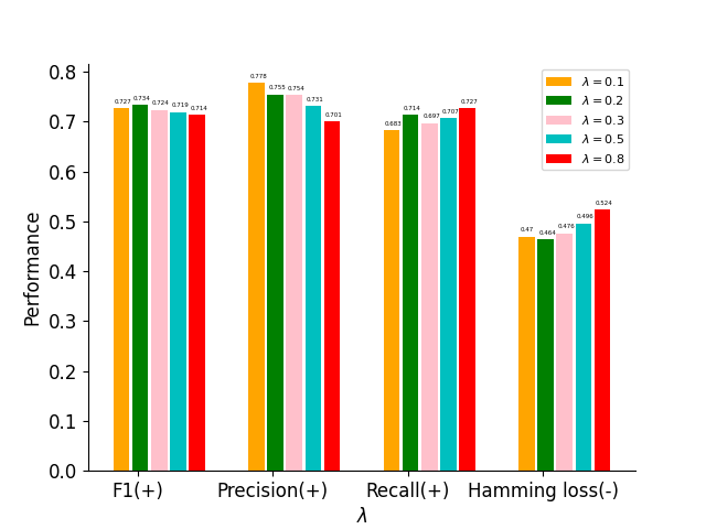
Figure 2: The performance of LD-SPN model on AAPD test set when using different $\lambda$. The Hamming loss is multiplied by 20. The symbol "+" indicates that the higer th value is, the better the model performs. The symbol "-" is the opposite.

Analysis of the Number of Decoder Layers

To evaluate the importance of the non-autoregressive decoder, we change the number of the decoder layers for MixATIS and AAPD datasets. As shown in Table 5, when the number of the decoder layers is set to 2 and 3, the better result of MixATIS dataset is obtained when the number of the decoder layers is 2 while for the AAPD dataset is 3. Since the number of labels in MixATIS is much less than that of the AAPD dataset, the more of the number of decoder layers may result in overfitting.

Dataset	LD-SPN
	#Decoder Layers	F1(+)	P(+)	R(+)	HL(-)
MixATIS	2	0.906	0.912	0.899	0.0198
	3	0.885	0.892	0.878	0.0241
AAPD	2	0.719	0.777	0.669	0.0234
	3	0.734	0.755	0.714	0.0229

Table 5: Ablation study for LD-SPN on the MixATIS and AAPD datasets. The number of decoder layers in the non-autoregressive decoder are set to 2 and 3, respectively.

Analysis of the Number of Query Labels

From the architecture of SPN for multilabel classification, we can see the number of output labels is equal to the number of query labels. The maximum number of labels in MixATIS and AAPD datasets are 3 and 8, respectively. We set the number of query for each dataset less than, equal and more than the maximum number of labels in them. Table 6 shows the results. We can see that increasing the number of query labels can achieve better or competitive results, which may be due to the bipartite matching loss function to measure the difference between the predicted and ground truth labels, it’s insensitive to the number of output labels. In reality, we should consider to choose a proper number for the query labels to computation efficiency and performance.

Dataset	LD-SPN
	#Query Labels	F1(+)	P(+)	R(+)	HL(-)
MixATIS	2	0.846	0.901	0.797	0.0307
	3	0.890	0.907	0.874	0.0227
	5	0.906	0.912	0.899	0.0198
AAPD	5	0.728	0.769	0.691	0.0232
	8	0.727	0.795	0.670	0.0231
	10	0.734	0.755	0.714	0.0229

Table 6: Ablation study for LD-SPN on the MixATIS and AAPD datasets. The maximum number of labels in MixATIS and AAPD datasets are 3 and 8, respectively.

Analysis of the Smoothing Thresholding Parameter for Adjacency Matrix

In order to show how the smoothing thresholding parameter of the adjacency matrix influence the model performance, we conduct experiments on MixATIS and AAPD datasets. From Table 7 we find that better result can be obtained through smoothing the adjacency matrix appropriately. Since each sample of the AAPD dataset has more labels than that of the MixATIS dataset, each label seems more sparse, it is suitable to set a bigger smoothing parameter.

Dataset	LD-SPN
	$\tau$	F1(+)	P(+)	R(+)	HL(-)
MixATIS	0	0.892	0.904	0.881	0.0224
	0.1	0.906	0.912	0.899	0.0198
	0.2	0.887	0.897	0.877	0.0236
AAPD	0	0.723	0.784	0.673	0.0232
	0.1	0.719	0.773	0.672	0.0236
	0.2	0.734	0.755	0.714	0.0229

Table 7: Ablation study for LD-SPN on the MixATIS and AAPD datasets. The adjacency matrix smoothing thresholding parameter $\tau$ is set to 0, 0.1 and 0.2, respectively.

5 Conclusion

In this paper we propose to employ the set prediction networks to solve the multi-label text classification, which can get rid of predicting the order of labels. Since the sentence and the label dependencies both influence the prediction results, a pretrained language model is used to encode the sentence, an adjacency matrix composed of the conditional probabilities between labels is computed to model the label correlation and GCN is utilized to propagation the information between labels. Then a non-autoregressive decoder takes both the sentence representation and label dependencies information as input and output the distributions of predicted labels. With the purpose of elevating the recall ability, the Bhattacharyya distance between the output distributions is optimized simultaneously with the bipartite matching loss function in set prediction. Experimental results show that our method can obtain beneficial performance with the baselines. Compared with the binary cross entropy loss and naive set prediction networks for multi-label text classification, ablation analyses show that the bipartite matching loss function used in set prediction, the combination of label dependencies information with sentence representation, the Bhattacharyya distance exerted on output distribution in our method all demonstrate its effectiveness.

References

- [1] Zichao Yang, Diyi Yang, Chris Dyer, Xiaodong He, Alex Smola, and Eduard Hovy. Hierarchical attention networks for document classification. In Proceedings of the 2016 conference of the North American chapter of the association for computational linguistics: human language technologies, pages 1480–1489, 2016.
- [2] Ankit Kumar, Ozan Irsoy, Peter Ondruska, Mohit Iyyer, James Bradbury, Ishaan Gulrajani, Victor Zhong, Romain Paulus, and Richard Socher. Ask me anything: Dynamic memory networks for natural language processing. In International conference on machine learning, pages 1378–1387. PMLR, 2016.
- [3] Erik Cambria, Daniel Olsher, and Dheeraj Rajagopal. Senticnet 3: a common and common-sense knowledge base for cognition-driven sentiment analysis. In Proceedings of the AAAI conference on artificial intelligence, volume 28, 2014.
- [4] Libo Qin, Xiao Xu, Wanxiang Che, and Ting Liu. Agif: An adaptive graph-interactive framework for joint multiple intent detection and slot filling. arXiv preprint arXiv:2004.10087, 2020.
- [5] Pengcheng Yang, Xu Sun, Wei Li, Shuming Ma, Wei Wu, and Houfeng Wang. Sgm: Sequence generation model for multi-label classification. In International Conference on Computational Linguistics, 2018.
- [6] M. R. Boutell, J. Luo, X. Shen, and C. M. Brown. Learning multi-label scene classification. Pattern Recognition, 37(9):1757–1771, 2004.
- [7] G. Tsoumakas and I. Katakis. Multi-label classification: An overview. International Journal of Data Warehousing and Mining, 3(3):1–13, 2009.
- [8] Li Li, Houfeng Wang, Xu Sun, Baobao Chang, Shi Zhao, and Lei Sha. Multi-label text categorization with joint learning predictions-as-features method. In Conference on Empirical Methods in Natural Language Processing, 2015.
- [9] Grigorios Tsoumakas and Ioannis P. Vlahavas. Random k -labelsets: An ensemble method for multilabel classification. In European Conference on Machine Learning, 2007.
- [10] S. Piotr, K. Tomasz, and K. Kristian. How is a data-driven approach better than random choice in label space division for multi-label classification? Entropy, 18(8), 2016.
- [11] Guibin Chen, Deheng Ye, Zhenchang Xing, Jieshan Chen, and E. Cambria. Ensemble application of convolutional and recurrent neural networks for multi-label text categorization. 2017 International Joint Conference on Neural Networks (IJCNN), pages 2377–2383, 2017.
- [12] Simon Baker and Anna Korhonen. Initializing neural networks for hierarchical multi-label text classification. In Workshop on Biomedical Natural Language Processing, 2017.
- [13] Jingzhou Liu, Wei-Cheng Chang, Yuexin Wu, and Yiming Yang. Deep learning for extreme multi-label text classification. In Proceedings of the 40th international ACM SIGIR conference on research and development in information retrieval, pages 115–124, 2017.
- [14] Gakuto Kurata, Bing Xiang, and Bowen Zhou. Improved neural network-based multi-label classification with better initialization leveraging label co-occurrence. In Proceedings of the 2016 Conference of the North American Chapter of the Association for Computational Linguistics: Human Language Technologies, pages 521–526, 2016.
- [15] Pengfei Liu, Xipeng Qiu, and Xuanjing Huang. Recurrent neural network for text classification with multi-task learning. arXiv preprint arXiv:1605.05101, 2016.
- [16] Siwei Lai, Liheng Xu, Kang Liu, and Jun Zhao. Recurrent convolutional neural networks for text classification. In Proceedings of the AAAI conference on artificial intelligence, volume 29, 2015.
- [17] Guibin Chen, Deheng Ye, Zhenchang Xing, Jieshan Chen, and Erik Cambria. Ensemble application of convolutional and recurrent neural networks for multi-label text categorization. In 2017 International joint conference on neural networks (IJCNN), pages 2377–2383. IEEE, 2017.
- [18] Ronghui You, Suyang Dai, Zihan Zhang, Hiroshi Mamitsuka, and Shanfeng Zhu. Attentionxml: Extreme multi-label text classification with multi-label attention based recurrent neural networks. arXiv preprint arXiv:1811.01727, 137:138–187, 2018.
- [19] Ashutosh Adhikari, Achyudh Ram, Raphael Tang, and Jimmy Lin. Docbert: Bert for document classification. arXiv preprint arXiv:1904.08398, 2019.
- [20] Wenjie Zhang, Junchi Yan, Xiangfeng Wang, and Hongyuan Zha. Deep extreme multi-label learning. In Proceedings of the 2018 ACM on international conference on multimedia retrieval, pages 100–107, 2018.
- [21] Cunxiao Du, Zhaozheng Chen, Fuli Feng, Lei Zhu, Tian Gan, and Liqiang Nie. Explicit interaction model towards text classification. In Proceedings of the AAAI conference on artificial intelligence, volume 33, pages 6359–6366, 2019.
- [22] Nikolaos Pappas and James Henderson. Gile: A generalized input-label embedding for text classification. Transactions of the Association for Computational Linguistics, 7:139–155, 2019.
- [23] Dianbo Sui, Yubo Chen, Kang Liu, Jun Zhao, Xiangrong Zeng, and Shengping Liu. Joint entity and relation extraction with set prediction networks. arXiv preprint arXiv:2011.01675, 2020.
- [24] Jacob Devlin, Ming-Wei Chang, Kenton Lee, and Kristina Toutanova. Bert: Pre-training of deep bidirectional transformers for language understanding. ArXiv, abs/1810.04805, 2019.
- [25] Jiatao Gu, James Bradbury, Caiming Xiong, Victor OK Li, and Richard Socher. Non-autoregressive neural machine translation. arXiv preprint arXiv:1711.02281, 2017.
- [26] A. Bhattacharyya. On a measure of divergence between two statistical populations defined by their probability distributions. volume 35, 1943.
- [27] Libo Qin, Xiao Xu, Wanxiang Che, and Ting Liu. Agif: An adaptive graph-interactive framework for joint multiple intent detection and slot filling. arXiv: Computation and Language, 2020.
- [28] Libo Qin, Wanxiang Che, Yangming Li, Haoyang Wen, and Ting Liu. A stack-propagation framework with token-level intent detection for spoken language understanding. ArXiv, abs/1909.02188, 2019.
- [29] Jiatao Gu, James Bradbury, Caiming Xiong, Victor O. K. Li, and Richard Socher. Non-autoregressive neural machine translation. ArXiv, abs/1711.02281, 2017.
- [30] Sepp Hochreiter and Jürgen Schmidhuber. Long short-term memory. Neural Computation, 9:1735–1780, 1997.
- [31] Jack Edmonds and Richard M. Karp. Theoretical improvements in algorithmic efficiency for network flow problems. Journal of the ACM (JACM), 19:248 – 264, 1972.
- [32] Nicolas Carion, Francisco Massa, Gabriel Synnaeve, Nicolas Usunier, Alexander Kirillov, and Sergey Zagoruyko. End-to-end object detection with transformers. ArXiv, abs/2005.12872, 2020.
- [33] Georg Hess, Christoffer Petersson, and Lennart Svensson. Object detection as probabilistic set prediction. ArXiv, abs/2203.07980, 2022.
- [34] P. Yang, S. Xu, L. Wei, S. Ma, and W. Wei. Sgm: Sequence generation model for multi-label classification. 2018.
- [35] Ashish Vaswani, Noam M. Shazeer, Niki Parmar, Jakob Uszkoreit, Llion Jones, Aidan N. Gomez, Lukasz Kaiser, and Illia Polosukhin. Attention is all you need. ArXiv, abs/1706.03762, 2017.
- [36] X. Li, F. Zhao, and Y. Guo. Multi-label image classification with a probabilistic label enhancement model. In Thirtieth Conference on Uncertainty in Artificial Intelligence, 2014.
- [37] Z. M. Chen, X. S. Wei, P. Wang, and Y. Guo. Multi-label image recognition with graph convolutional networks. In 2019 IEEE/CVF Conference on Computer Vision and Pattern Recognition (CVPR), 2019.
- [38] Z. Wu, S. Pan, F. Chen, G. Long, C. Zhang, and P. S. Yu. A comprehensive survey on graph neural networks. IEEE transactions on neural networks and learning systems, (1):32, 2021.
- [39] H. Wang, Y. Zou, D. Chong, and W. Wang. Modeling label dependencies for audio tagging with graph convolutional network. IEEE Signal Processing Letters, PP(99):1–1, 2020.
- [40] Alice Coucke, Alaa Saade, Adrien Ball, Théodore Bluche, Alexandre Caulier, David Leroy, Clément Doumouro, Thibault Gisselbrecht, Francesco Caltagirone, Thibaut Lavril, Maël Primet, and Joseph Dureau. Snips voice platform: an embedded spoken language understanding system for private-by-design voice interfaces. ArXiv, abs/1805.10190, 2018.
- [41] Charles T. Hemphill, John J. Godfrey, and George R. Doddington. The atis spoken language systems pilot corpus. In Human Language Technology - The Baltic Perspectiv, 1990.
- [42] David D. Lewis, Yiming Yang, Tony G. Rose, and Fan Li. Rcv1: A new benchmark collection for text categorization research. J. Mach. Learn. Res., 5:361–397, 2004.
- [43] Robert E. Schapire and Yoram Singer. Improved boosting algorithms using confidence-rated predictions. Machine Learning, 37:297–336, 1998.
- [44] Christopher D. Manning, Prabhakar Raghavan, and Hinrich Schütze. Introduction to information retrieval. 2008.
- [45] Diederik P. Kingma and Jimmy Ba. Adam: A method for stochastic optimization. CoRR, abs/1412.6980, 2014.