Estimating Conditional Average Treatment Effects with Heteroscedasticity by Model Averaging and Matching

Abstract

Causal inference is indispensable in many fields of empirical research, such as marketing, economic policy, medicine and so on. The estimation of treatment effects is the most important in causal inference. In this paper, we propose a model averaging approach, combined with a partition and matching method to estimate the conditional average treatment effect under heteroskedastic error settings. In our methods, we use the partition and matching method to approximate the true treatment effects and choose the weights by minimizing a leave-one-out cross validation criterion, which is also known as jackknife method. We prove that the model averaging estimator with weights determined by our criterion has asymptotic optimality, which achieves the lowest possible squared error. When there exist correct models in the candidate model set, we have proved that the sum of weights of the correct models converge to 1 as the sample size increases but with a finite number of baseline covariates. A Monte Carlo simulation study shows that our method has good performance in finite sample cases. We apply this approach to a National Supported Work Demonstration data set.

1 Introduction

Causal inference is essential to empirical investigations, in which the estimation of treatment effects on the outcome is a key point. For example, in the field of medicine, we can estimate the treatment effects to investigate whether a new drug is effective. Furthermore, a treatment effect on the outcome can be heterogeneous with respect to some baseline covariates, that is we should derive a conditional treatment effects given some certain covariates. For the previous example, we can study different treatment effects of the new drug for person with different body qualifications, where the body qualifications are called “baseline covariates” in this case. There is a lot of literature on the estimation of treatment effects. For example, Ashenfelter, (1978), LaLonde, (1986), Abadie and Imbens, (2011), Cai et al., (2011), Fan et al., (2022) and many others. Several approaches and several models for estimating treatment effects have been developed. Naturally, to deal model uncertainty in estimating treatment effect, Rolling and Yang, (2014) proposed a treatment effect cross validation (TECV) method to select the model within a candidate model set that is globally the most accurate for estimating the treatment effects. Different from traditional cross validation, of which the goal is prediction, this approach aims to estimate the treatment effects.

Instead of selecting one specific model, we consider a model averaging approach, which incorporates model uncertainty into the estimation process. One of the biggest benefits is that model averaging estimator can reduce the risk in estimation because it provides a kind of insurance against selecting a poor model. Model averaging includes Bayesian model averaging (BMA) and frequentist model averaging (FMA). Hoeting et al., (1999) provided a very detailed introduction for the Bayesian model averaging and we focus on the latter. Weight choice is the key point for frequentist model averaging. On the one hand, several approaches determine the weights based on some measures so that there exists explicit expression. For example, Buckland et al., (1997) choosed weights based on information scores and proposed Smoothed AIC. On the other hand, there are lots of literature to select the weights towards some form of optimality. Hansen, (2007) and Wan et al., (2010) proposed least squares model averaging by Mallow’s criterion. Hansen and Racine, (2012) and Zhang et al., (2013) developed jackknife model averaging, which chooses weights based on a cross validation criterion. Lu and Su, (2015) utilized the idea of jackknife model averaging in quantile regressions. Zhang et al., (2015) proposed Kullback-Leibler type measures. Zhang et al., (2016) extended the model averaging to generalized linear models. In addition, Yang, (2001) and Yuan and Yang, (2005) proposed adaptive regression by mixing (ARM). There are also studies aiming at inference after model averaging (Hjort and Claeskens, (2003); Liu, (2015); Zhang and Liu, (2019)).

All the above model averaging approaches are to improve the accuracy of prediction. There are few studies for the estimation of treatment effects. Kitagawa and Muris, (2016) minimised the approximated mean squared error of a semiparametric estimator in terms of treatment effects based on a model averaging method. They proved that this approach is Bayes optimal given a certain prior. Antonelli and Cefalu, (2020) proposed averaging causal estimators in high dimensions which merges multiple models in different frameworks. However, they did not give theoretical proofs about the effects of their estimators. Rolling et al., (2019) developed a method of model combination that targets accurate estimation of the treatment effect conditional on some certain covariates, which is also known as treatment effect estimation by mixing (TEEM). They provided a risk bound for their estimator under squared error loss but there is no asymptotic optimality. Zhao et al., (2021) developed a weight choice method based on minimization of the approximate risk under squared error loss and proved this estimator has an optimal asymptotic property. However, their study is constructed on the homoskedastic error settings and they only consider the cases, where all the candidate models are misspecified, that is, they didn’t derive the properties when there exist correct candidate models in the candidate model set.

In this paper, we consider the problem of estimating treatment effects on the response variable under heteroskedastic error settings, which is often encountered. The approach proposed by Zhao et al., (2021) chooses weights by a criterion similar to the Mallow’s Cp criterion, which can only solve the problem under homoskedastic error settings. In reality, the data set may exist heteroscedasticity, that is, not all the noises of the observations have the same variance. In our weight choice criterion, we firstly use the partition and matching method introduced by Rolling and Yang, (2014) to approximate the true treatment effects, then minimize the mean squared error of leave-one-out cross validation, which is also known as the jackknife method. Allen, (1974), Stone, (1974) and Wahba and Wold, (1975) developed selection of regression models based on leave-one-out cross validation criterion. Li, (1987) proved the optimality for homoskedastic regression and Andrews, (1991) proved optimality for heteroskedastic regression. Based on the theory developed in Li, (1987) and Wan et al., (2010), we derived the asymptotic optimality under heteroskedastic error settings. Furthermore, we also derived the asymptotic property of weights, which has not been studied in the aforementioned articles on estimating treatments effect using model averaging. On the one hand, when all the candidate models are misspecified, the model averaging estimators with weight choosed by our cross validation criterion has the asymptotic optimality, that is, it achieves the lowest possible squared error among all the combination of these candidate models. On the other hand, when there exist correct models, the sum of the weights assigned to these correct models converges to 1 as the sample size increases. These two properties insure that our model averaging estimator can perform the best no matter what the candidate models are.

The remainder of this paper is organized as follows. The model framework is presented in Section 2. Section 3 introduces the model averaging estimator, our weight choice criterion. The asymptotic properties are presented in Section 4. A Monto Carlo simulation study is presented in Section 5 to show the finite sample performance of our approach. Section 6 is a real data example, which applies our approach to a National Supported Work Demonstration data set. The results of simulation and the technical proofs are given in the Appendix.

2 Model Framework

We consider a general regression framework in which the response $Y$ is dependent on a binary treatment variable $T\in\{t,c\}$, where $T=t$ and $T=c$ represent the individual being under treatment and under control, respectively and some baseline covariates $\mathbf{u}\in\mathbb{R}^{p}$. The data generating process can be written as follows:

$$Y_{i}=[f_{t}(\mathbf{u}_{i})+\zeta_{i}]I(T_{i}=t)+[f_{c}(\mathbf{u}_{i})+\nu_{i}]I(T_{i}=c),$$ (2.1)

where $\mathbf{u}_{i}$ are independent and identically distributed (IID) from some unknown distribution $P_{\mathbf{U}}$ with support $\mathcal{U}\subset\mathbb{R}^{p}$. The random errors under treatment are denoted as $\zeta_{i}$, and $\nu_{i}$ are the random errors under control, where we assume a heteroskedastic error setting, hence

$$\operatorname*{E}(\zeta_{i}\mid\mathbf{u}_{i})=\operatorname*{E}(\nu_{i}\mid\mathbf{u}_{i})=0,~{}~{}~{}\zeta_{i}\perp\nu_{i}\text{ for }i=1,2,...$$ (2.2)

and

$$\operatorname*{E}(\zeta_{i}^{2}\mid\mathbf{u}_{i})=\sigma_{i,t}^{2},~{}~{}~{}\operatorname*{E}(\nu_{i}^{2}\mid\mathbf{u}_{i})=\sigma_{i,c}^{2}\text{ for }i=1,2,...,$$ (2.3)

which allows that the errors under treatment and control have different variances over different units.

Our goal is to estimate $\Delta(\mathbf{u}):=f_{t}(\mathbf{u})-f_{c}(\mathbf{u})$, the difference in the regression functions between the treatment group and control group since several literatures interpret $\Delta(\mathbf{u})$ as the causal effect under some conditions (Imbens and Wooldridge, 2009 and Rolling and Yang, 2014). Let $Y_{i,t}$ and $Y_{i,c}$ be the potential outcomes under treatment and control, respectively, then the causal effect of the treatment $T$ on the unit $i$ is $Y_{i,t}-Y_{i,c}$, but we can not obesrve both $Y_{i,t}$ and $Y_{i,c}$ simultaneously. Typically, treatment effects are heterogeneous with respect to the baseline covariates, thus we define the conditional average treatment effect (CATE) as follows:

$$\text{CATE}(\mathbf{u}):=\operatorname*{E}[(Y_{i,t}-Y_{i,c})\mid\mathbf{u}_{i}=\mathbf{u}].$$ (2.4)

Note that $\Delta(\mathbf{u})=\operatorname*{E}(Y_{i}\mid T_{i}=t,\mathbf{u}_{i}=\mathbf{u})-\operatorname*{E}(Y_{i}\mid T_{i}=c,\mathbf{u}_{i}=\mathbf{u})$, which represents the conditional average treatment difference (CATD). To connect CATE with CATD, we then assume the following condition:

Condition 2.1 (Unconfounded assignment).

$\{Y_{i,t},Y_{i,c}\}\perp T_{i}\mid\mathbf{u}_{i}$.

This condition means that given the baseline covariates, the potential outcomes are independent with the treatment variable, that is all the confounding information are required to be contained in the baseline covariates. Under the unconfounded assignment, we have that

$$\text{CATE}(\mathbf{u})=f_{t}(\operatorname*{\mathbf{u}})-f_{c}(\operatorname*{\mathbf{u}}):=\Delta(\operatorname*{\mathbf{u}}).$$ (2.5)

Therefore, $\Delta(\mathbf{u})$ represents the average causal effect of treatment $T$ given some certain covariates value $\mathbf{u}$. This condition is always valid in randomized experiments but it is typically unknown whether this condition holds in observational studies. Rolling and Yang (2014) remarked that it is more plausible as the number of the baseline covariates increases. In this work, we focus on estimating $\Delta(\mathbf{u})$ because it is identifiable in most experiments and observational studies and we will refer to $\Delta(\mathbf{u})$ as the treatment effect during the remainder of this paper.

3 Model Averaging Estimation

3.1 Model averaging estimator

We consider $K$ candidate models, which utilize different $K$ subsets of $\mathbf{u}_{i}$. Denote the $i$-th vector of the covariates matrix in the $k$-th candidate model as $\mathbf{u}_{i}^{k}=(u_{1i}^{k},...,u_{p_{k}i}^{k})^{T}$, where $p_{k}$ is the number of covariates used in the $k$-th candidate model. For simplicity, we consider a linear model, then the $k$-th candidate model can be written by

$$Y_{i}=[\mathbf{u}_{i}^{k^{T}}\boldsymbol{\beta}^{k}+\zeta_{i}]I(T_{i}=t)+[\mathbf{u}_{i}^{k^{T}}\boldsymbol{\gamma}^{k}+\nu_{i}]I(T_{i}=c),~{}~{}i=1,...,n,$$ (3.1)

where $\boldsymbol{\beta}^{k}$ and $\boldsymbol{\gamma}^{k}$ are the parameter in the $k$-th model to be estimated. In addition, we can add polynomial forms or other functional forms of the covariates to the model to realize non-linear analysis.

Let $\mathbf{Y}_{ta}(n_{t}\times 1)$ be the response vector in the treatment group with length $n_{t}$ and $\mathbf{Y}_{ca}(n_{c}\times 1)$ be the response vector of in the control group with length $n_{c}$. Denote the covariates matrix corresponding to treatment and control groups as $\mathbf{U}_{ta}^{k}(n_{t}\times p_{k})$ and $\mathbf{U}_{ca}^{k}(n_{c}\times p_{k})$ respectively. We assume that $\mathbf{U}_{ta}^{k}$ and $\mathbf{U}_{ca}^{k}$ are of full column rank. Our primary focus will be on least-square estimators, in which case

$$\hat{\boldsymbol{\beta}}^{k}=(\mathbf{U}_{ta}^{k^{T}}\mathbf{U}_{ta}^{k})^{-1}\mathbf{U}_{ta}^{k^{T}}\mathbf{Y}_{ta},~{}~{}~{}~{}\hat{\boldsymbol{\gamma}}^{k}=(\mathbf{U}_{ca}^{k^{T}}\mathbf{U}_{ca}^{k})^{-1}\mathbf{U}_{ca}^{k^{T}}\mathbf{Y}_{ca}.$$ (3.2)

Then the estimator of the treatment effect $\Delta(\mathbf{u}_{i})$ under the $k$-th candidate model is the difference in the regressed functions between treatment and control groups,

$$\hat{\Delta}^{k}(\mathbf{u}_{i})=\mathbf{u}_{i}^{k^{T}}\hat{\boldsymbol{\beta}}^{k}-\mathbf{u}_{i}^{k^{T}}\hat{\boldsymbol{\gamma}}^{k}.$$ (3.3)

Thus, we assign the $k$-th candidate model with weight $w_{k}$ and the model averaging estimator can be written as

$$\hat{\Delta}_{i}(\operatorname*{\mathbf{w}})=\sum_{k=1}^{K}w_{k}\hat{\Delta}^{k}(\mathbf{u}_{i}),$$ (3.4)

where $\operatorname*{\mathbf{w}}=(w_{1},...,w_{K})^{\prime}$ is a weight vector belonging to the set

$$Q_{n}=\left\{\operatorname*{\mathbf{w}}\in[0,1]^{K}:\sum_{k=1}^{K}w_{k}=1\right\}.$$

We will discuss that how to choose the weight $\operatorname*{\mathbf{w}}$ in the next subsection.

3.2 Weight choice criterion

Before the treatment effects estimation, we utilize the “partition and match” idea in Rolling and Yang, (2014). In specific, we partition the feature space into lots of cells. Without loss of generality, we let the support of the probability density of $\mathbf{u}$ be $[0,1]^{p}$. Then we partition the feature space into $M$ cells with side length $h$. Next, in the $m$-th cell $(m=1,...,M)$, we can randomly choose a pair of observations $(m,m^{*})$ such that $T_{m}=t$ and $T_{m^{*}}=c$, which means that there are a treatment observation and a control observation in each pair. Denote $\mathbf{u}_{m}^{t}$ and $\mathbf{u}_{m}^{c}$ as the covariate vectors corresponding to the treatment observation and control observation in the $m$-th pair, respectively. Since these two observations come from the same cell, $\mathbf{u}_{m}^{t}$ and $\mathbf{u}_{m}^{c}$ have strong similarity. If we let $b_{m}=f_{c}(\mathbf{u}_{m}^{t})-f_{c}(\mathbf{u}_{m}^{c})$, $b_{m}$ will be very small, which is close to 0. Let $Y_{m}^{t},Y_{m}^{c},\zeta_{m}^{t},\nu_{m}^{c}$ be the corresponding responses and errors respectively, and $\eta_{m}=\zeta_{m}^{t}-\nu_{m}^{c}$. It is reasonable to approximate $\Delta({\mathbf{u}_{m}^{t}})$ by $Y_{m}^{t}-Y_{m}^{c}$, which has an approximation bias term $b_{m}$ and an error term $\eta_{m}$ additionally. Furthermore, if we use the side length $h$ suggested in Rolling and Yang, (2014), the approximation bias $b_{m},m=1,...,M$ have a uniform bound

$$\sup_{1\leq m\leq M}|b_{m}|=O\left(p\left(\frac{\log n}{n}\right)^{1/p}\right),$$ (3.5)

which provides insurance for the accuracy of our estimator.

In this paper, we propose a jackknife selection of $\mathbf{w}$, which is also known as leave-one-out cross validation. The $k$-th jackknife estimator for $\boldsymbol{\Delta}$ is $\tilde{\boldsymbol{\Delta}}^{k}=(\tilde{\Delta}^{k}(\mathbf{u}_{1}^{t}),...,\tilde{\Delta}^{k}(\mathbf{u}_{M}^{t}))^{\prime}$, where $\tilde{\Delta}^{k}(\mathbf{u}_{i}^{t})$ is the estimator $\hat{\Delta}^{k}(\mathbf{u}_{i}^{t})$ computed with the $i$-th observation deleted, and $\tilde{\boldsymbol{\Delta}}(\mathbf{w})=\sum_{k=1}^{K}w_{k}\tilde{\boldsymbol{\Delta}}^{k}$. Let $\mathbf{U}_{t}^{k}$ and $\mathbf{U}_{c}^{k}$ be the covariate matrices of the $k$-th candidate model corresponding to the treatment and control respectively, which both have dimensions $M\times p_{k}$. Let $\mathbf{Y}_{t}$ and $\mathbf{Y}_{c}$ be the responses corresponding to the treatment and control respectively. Let

$$\tilde{Y}_{m}=Y_{m}^{t}-Y_{m}^{c}, ~{}~{}~{}\tilde{\mathbf{Y}}=(\tilde{Y}_{1},...,\tilde{Y}_{M})^{\prime},$$

$$P_{t}^{(k)}=\mathbf{U}_{t}^{k}(\mathbf{U}_{t}^{k^{\prime}}\mathbf{U}_{t}^{k})^{-1}\mathbf{U}_{t}^{k^{\prime}}, ~{}~{}~{}P_{c}^{(k)}=\mathbf{U}_{t}^{k}(\mathbf{U}_{c}^{k^{\prime}}\mathbf{U}_{c}^{k})^{-1}\mathbf{U}_{c}^{k^{\prime}},$$

$$P_{t}(\operatorname*{\mathbf{w}})=\sum_{k=1}^{K}w_{k}P_{t}^{(k)}, ~{}~{}~{}P_{c}(\operatorname*{\mathbf{w}})=\sum_{k=1}^{K}w_{k}P_{c}^{(k)},$$ (3.6)

and the jackknife estimator $\tilde{{\Delta}}^{k}(\mathbf{u}_{i}^{t})$ can be written as

$$\tilde{{\Delta}}^{k}(\mathbf{u}_{i}^{t})=\mathbf{U}_{t,i}^{k}(\mathbf{U}_{t,-i}^{k^{\prime}}\mathbf{U}_{t,-i}^{k})^{-1}\mathbf{U}_{t,-i}^{k^{\prime}}\mathbf{Y}_{t,-i}-\mathbf{U}_{t,i}^{k}(\mathbf{U}_{c,-i}^{k^{\prime}}\mathbf{U}_{c,-i}^{k})^{-1}\mathbf{U}_{c,-i}^{k^{\prime}}\mathbf{Y}_{c,-i},$$ (3.7)

where $\mathbf{U}_{t,i}^{k}$ is the $i$-th row of $\mathbf{U}_{t}^{k}$, and $\mathbf{U}_{t,-i}^{k}$, $\mathbf{U}_{c,-i}^{k}$ are the matrices $\mathbf{U}_{t}^{k}$, $\mathbf{U}_{c}^{k}$ with the $i$-th row deleted respectively. $\mathbf{Y}_{t,-i}$ and $\mathbf{Y}_{c,-i}$ are the responses $\mathbf{Y}_{t}$, $\mathbf{Y}_{c}$ with the $i$-th element deleted. Thus we can write

$$\tilde{\boldsymbol{\Delta}}^{k}=\tilde{P}_{t}^{(k)}\mathbf{Y}_{t}-\tilde{P}_{c}^{(k)}\mathbf{Y}_{c}$$ (3.8)

and

$$\tilde{\boldsymbol{\Delta}}(\operatorname*{\mathbf{w}})=\sum_{k=1}^{K}w_{k}\tilde{\boldsymbol{\Delta}}^{k}=\sum_{k=1}^{K}w_{k}(\tilde{P}_{t}^{(k)}\mathbf{Y}_{t}-\tilde{P}_{c}^{(k)}\mathbf{Y}_{c}),$$ (3.9)

where $\tilde{P}_{t}^{(k)}$ and $\tilde{P}_{c}^{(k)}$ have zeros on the diagonal and dependens only on $\operatorname*{\mathbf{u}}$. Then we propose the weight choice criterion based on the residuals of the jackknife averaging estimator:

$$\hat{\mathbf{w}}=\mathop{\arg\min}_{\operatorname*{\mathbf{w}}\in Q_{n}}~{}\text{CV}(\operatorname*{\mathbf{w}})=\mathop{\arg\min}_{\operatorname*{\mathbf{w}}\in Q_{n}}~{}||\tilde{\boldsymbol{\Delta}}(\operatorname*{\mathbf{w}})-\tilde{\mathbf{Y}}||^{2}.$$ (3.10)

We take this chosen weights to (3.4) and obtain the jackknife model averaging estimator of the treatment effects $\hat{\Delta}_{i}(\operatorname*{\mathbf{w}})=\sum_{k=1}^{K}\hat{w}_{k}\hat{\Delta}^{k}(\mathbf{u}_{i})$ and we label our method as JMA. We give the algorithm of our approach as follows:

Algorithm 1 Estimating CATE via jackknife model averaging

  Input:

  •data $(\mathbf{U},\mathbf{Y})$;

  •K subsets $\mathbf{u}^{k},k=1,...,K$ included in the $K$ candidate models respectively;

  •the number of pairs of observations $M$.

  Output: the estimator of conditional average treatment effect $\hat{\Delta}(\operatorname*{\mathbf{w}})$.

  Step 0: use the subset $\mathbf{u}^{k}$ to obtain the OLS estimators $\hat{\boldsymbol{\beta}}^{k}$ and $\hat{\boldsymbol{\gamma}}^{k}$ by (3.2) for $k=1,...,K$.

  Step 1: use the “partition and match” method to select $M$ pairs of observations from the original data set and calculate the difference of their response as the ”true” treatment effect $\tilde{\mathbf{Y}}=(\tilde{Y}_{1},...,\tilde{Y}_{M})^{\prime}$.

  Step 2: calculate the jackknife prediction error

  for m = 1:M do

     •remove the $m$-th pair of observations from the original data set and fit the $k$-th model using $\mathbf{u}^{k}$ as its predictors for $k=1,...,K$.

     •use the $k$-th candidate model to predict the treatment effect of the $m$-th treatment observation, recorded as $\tilde{\Delta}_{m}^{k}$ for $k=1,...,K$.

     •average the $K$ predicted values, denoted as $\tilde{\Delta}_{m}(\operatorname*{\mathbf{w}})=\sum_{k=1}^{K}w_{k}\tilde{\Delta}_{m}^{k}$.

  end forThen we obtain that $\tilde{\boldsymbol{\Delta}}(\operatorname*{\mathbf{w}})=(\tilde{\Delta}_{1}(\operatorname*{\mathbf{w}}),...,\tilde{\Delta}_{M}(\operatorname*{\mathbf{w}}))^{\prime}$.

  Step 3: calculate the optimal weight $\hat{\mathbf{w}}$ based on the criterion (3.10).

  Step 4: take the optimal weights $\hat{\mathbf{w}}$ into (3.4) and we obtain the estimator for CATE.

4 Asymptotic Properties

4.1 Asymptotic optimality

Let $\hat{\boldsymbol{\Delta}}^{k}=(\hat{\Delta}^{k}(\mathbf{u}_{1}^{t}),...,\hat{\Delta}^{k}(\mathbf{u}_{M}^{t}))^{\prime}$, $\hat{\boldsymbol{\Delta}}(\mathbf{w})=\sum_{k=1}^{K}w_{k}\hat{\boldsymbol{\Delta}}^{k}$, and $\boldsymbol{\Delta}=(\Delta(\mathbf{u}_{1}^{t}),...,\Delta(\mathbf{u}_{M}^{t}))^{\prime}$. Define the squared error of $\hat{\boldsymbol{\Delta}}(\operatorname*{\mathbf{w}})$ as $L_{n}(\mathbf{w})=||\hat{\boldsymbol{\Delta}}(\mathbf{w})-\boldsymbol{\Delta}||^{2}$ and the corresponding conditional risk as $R_{n}(\mathbf{w})=\operatorname*{E}[L_{n}(\mathbf{w})\mid\mathbf{u}]$. Let $\tilde{L}_{n}(\mathbf{w})=||\tilde{\boldsymbol{\Delta}}(\mathbf{w})-\boldsymbol{\Delta}||^{2}$ and $\tilde{R}_{n}(\mathbf{w})=\operatorname*{E}[\tilde{L}_{n}(\mathbf{w})\mid\mathbf{u}]$ be the jackknife squared error loss and risk respectively. Let $\xi_{n}=\mathop{\inf}_{\operatorname*{\mathbf{w}}\in Q_{n}}R(\operatorname*{\mathbf{w}})$ and $\tilde{\xi}_{n}=\mathop{\inf}_{\operatorname*{\mathbf{w}}\in Q_{n}}\tilde{R}(\operatorname*{\mathbf{w}})$. Denote $\bar{\lambda}(\mathbf{A})$ as the maximal diagonal element of a matrix $\mathbf{A}$. Let $\mathbf{w}_{k}^{0}$ be the vector with the $k$-th element being 1 and other elements taking on the value of 0. Before introducing the asymptotic optimality, we give some conditions.

Condition 4.1.

$\sup_{\operatorname*{\mathbf{w}}\in Q_{n}}|\tilde{R}_{n}(\operatorname*{\mathbf{w}})/R_{n}(\operatorname*{\mathbf{w}})-1|\stackrel{{\scriptstyle a.s.}}{{\longrightarrow}}0.$

Condition 4.2.

$K\xi_{n}^{-2G}\sum_{k=1}^{K}\left(R_{n}(\mathbf{w}_{k}^{0})\right)^{G}\stackrel{{\scriptstyle a.s.}}{{\longrightarrow}}0$, where $G$ is a constant that $G\geq 1$.

Condition 4.3.

$\sup_{k}\frac{1}{p_{k}}\bar{\lambda}(P_{t}^{(k)})\leq\Lambda n^{-1}$ and $\sup_{k}\frac{1}{p_{k}}\bar{\lambda}(P_{c}^{(k)})\leq\Lambda n^{-1}$, where $\Lambda$ is a finite constant.

Condition 4.4.

$\frac{K\cdot p^{1/2}\cdot n^{1/2}}{\tilde{\xi}_{n}}\rightarrow 0.$

Remark 4.1.

Condition 4.1 means that the difference between the risk of the regular and jackknife estimators goes to zero uniformly over all the averaging estimators as the sample size becomes large, which is standard in cross-validation analysis. Condition 4.2 is also required in Wan et al., (2010) and Zhang et al., (2013). It means that $\xi_{n}$ will go to infinity with $n$ and also places a restriction that the number of candidate models $K$ can not increase too fast. Condition 4.3, which is the same as condition (5.2) of Li, (1987) and also required in Ando and Li, (2014). This condition is always valid except for the design matrices being extremely unbalanced. Condition 4.4 sets an upper bound on the number of candidate models and the number of covariates. If the number of covariates $p$ is fixed and assume the order of $\tilde{\xi}_{n}$ is $n^{1-\delta}$, then $K$ is allowed to grow to infinity if $\delta<1/2$. That is, we need $\tilde{\xi}_{n}$ to grow at a rate no slower than $n^{1/2}$ to allow the number of candidate models $K$ to increase to infinity as the sample size increases.

Theorem 4.1 (Asymptotic Optimality).

Suppose that conditions (4.1)-(4.4) hold. Then our averaging estimator has the asymptotic optimality in the sense of mean squared error as $n\rightarrow\infty$,

$$\frac{L(\hat{\mathbf{w}})}{\mathop{\inf}_{\mathbf{w}\in Q_{n}}L(\mathbf{w})}\rightarrow 1.$$ (4.1)

Proof: See Appendix D.

This property is necessary in the model averaging estimator. Hansen, (2007) and Wan et al., (2010) proved this property in linear regression model under homoskedastic error settings. Hansen and Racine, (2012) and Zhang et al., (2013) extended this property to the heteroskedastic error settings. Zhao et al., (2021) proved this property under homoskedastic error settings in terms of treatment effect estimations and we prove it under heteroscedasticity.

4.2 Weight consistency

In this subsection, we consider the special case, in which the number of baseline covariates is finite. We firstly expand the vector $\hat{\boldsymbol{\beta}}^{k}$, $\hat{\boldsymbol{\gamma}}^{k}$, $\tilde{\boldsymbol{\beta}}^{k}$ and $\hat{\boldsymbol{\gamma}}^{k}$ to $p$ dimensions by adding $p-p_{k}$ zero elements to the end of the original vectors. Let $\boldsymbol{\beta}^{k^{*}}$ and $\boldsymbol{\gamma}^{k^{*}}$ be the limiting values of $\hat{\boldsymbol{\beta}}^{k}$ and $\hat{\boldsymbol{\gamma}}^{k}$, $\boldsymbol{\Delta}^{k^{*}}=\mathbf{U}_{t}\boldsymbol{\beta}^{k^{*}}-\mathbf{U}_{t}\boldsymbol{\gamma}^{k^{*}}$ and $\boldsymbol{\Delta}^{*}(\operatorname*{\mathbf{w}})=\sum_{k=1}^{K}w_{k}\boldsymbol{\Delta}^{k^{*}}$.

Let the subset $S\subseteq\{1,...,K\}$ includes the indices of the correct models, and $|S|=k_{0}\leq K$. Without loss of generality, we can assume that the first $k_{0}$ models are correct. Denote $\hat{w}_{\Delta}=\sum_{k=1}^{k_{0}}\hat{w}_{k}$ as the sum of the weights of all the correct candidate models, where $\hat{w}_{k}$ is the weight of the $k$-th model. Denote $Q_{F}=\{\operatorname*{\mathbf{w}}_{F}\in Q_{n}:\sum_{k=k_{0}+1}^{K}w_{F,k}=1\}$ as the weight set that assign all the weights to the wrong models. Let $\xi_{F}=\inf_{\operatorname*{\mathbf{w}}_{F}\in Q_{F}}L^{*}(\operatorname*{\mathbf{w}}_{F})$, where $L^{*}(\operatorname*{\mathbf{w}}_{F})=||\boldsymbol{\Delta}^{*}(\operatorname*{\mathbf{w}}_{F})-\boldsymbol{\Delta}||^{2}$. Since we use the idea of partition and match, we constructed the approximate treatment effect by $\tilde{Y}_{i}=\Delta_{i}+b_{i}+\eta_{i}$, where $\eta_{i}=\zeta_{i}^{t}-\nu_{i}^{c}$.

To consider the limiting property of the model weights, we hope that $\hat{w}_{\Delta}$ can be as large as possible, that is we can assign lots of the weights to the correct models. Firstly, we give some conditions.

Condition 4.5.

For any $\hat{\boldsymbol{\beta}}^{k}$ and $\hat{\boldsymbol{\gamma}}^{k}$, there exist the limit $\boldsymbol{\beta}^{k^{*}}$ and $\boldsymbol{\gamma}^{k^{*}}$ such that

$$\hat{\boldsymbol{\beta}}^{k}-\boldsymbol{\beta}^{k^{*}}=O_{p}(n^{-1/2}),~{}~{}~{}\hat{\boldsymbol{\gamma}}^{k}-\boldsymbol{\gamma}^{k^{*}}=O_{p}(n^{-1/2}).$$

Condition 4.6.

$\vartheta(n^{-1}\mathbf{U}_{t}^{T}\mathbf{U}_{t})=O(1)$, where $\vartheta(\mathbf{A})$ denotes the largest singular value of a matrix $\mathbf{A}$.

Condition 4.7.

Assume that there exists a constant $\phi>0$ such that $\sup_{1\leq i\leq n}\operatorname*{E}(|\eta_{i}|^{2+\phi})<\delta_{1}$, $n^{-1}\sum_{i=1}^{n}|\Delta^{k^{*}}_{i}|^{2+\phi}<\delta_{2}$ for $k=1,...,k_{0}$ and $n^{-1}\sum_{i=1}^{n}|\Delta_{i}|^{2+\phi}<\delta_{3}$, where $\delta_{i}<\infty$ for $i=1,2,3$ are positive constants.

Condition 4.8.

$\xi_{F}^{-1}n^{1/2}=o(1)$.

Remark 4.2.

Condition 4.5 means that the rate of convergence of $\hat{\boldsymbol{\beta}}^{k}$ and $\hat{\boldsymbol{\gamma}}^{k}$ to their limits $\boldsymbol{\beta}^{k^{*}}$ and $\boldsymbol{\gamma}^{k^{*}}$ should be slower than or equal to $n^{-1/2}$. This condition is valid when we use maximum likelihood method for estimation under model misspecification, which is derived from White (1982). Condition 4.6 places a condition on the maximal singular value of $n^{-1}\mathbf{U}_{t}^{T}\mathbf{U}_{t}$. Condition 4.7 places a restriction on the $2+\phi$ order moments of the error term. Meanwhile we also place a constraint on the moments of the limit of estimators and true treatment effects. Condition 4.8 requires that $\xi_{F}^{-1}\rightarrow\infty$ and also needs $\xi_{F}^{-1}$ goes to infinity at a faster rate than $n^{1/2}$. This condition is reasonable since if we assign all the weights to the wrong models, the conditional risk will go to infinity with a fast rate.

Theorem 4.2 (Consistency of weight).

Suppose Conditions (4.5)-(4.8) hold. Then, as $n\rightarrow\infty$

$$\hat{w}_{\Delta}\overset{p}{\longrightarrow}1.$$ (4.2)

Proof: See Appendix E.

Therefore, Theorem 1 and Theorem 2 guarantee that when there is no correct model in the candidate model set, the proposed estimator achieves the lowest possible squared error and when there exist correct models in the candidate model set, the sum of the weights of the correct candidate models converges to 1 as the sample size increases.

5 Monte Carlo Study

Before stating the simulation results, we introduce the nearest neighbour pairing method, which is widely used in the practical problems. We firstly scale the covariates so that each covariate has common mean and variance and the standardised covariates are denoted as $\tilde{\mathbf{U}}$. Secondly, for each observation in the treatment group, we find an observation in control group, who has a smallest distance with it, where we calculate the distance based on the standardised covariates, that is why we call it “nearest neighbour pairing”. Specifically, for the $i$-th observation in the treatment group ($i=1,2,...,n_{t}$), we find an observation in the control group by

$$i^{*}=\arg\min_{1\leq j\leq n_{c}}d(\tilde{\mathbf{U}}_{i},\tilde{\mathbf{U}}_{j}),~{}~{}~{}~{}\text{s.t.}~{}~{}~{}~{}T_{i}\neq T_{j},$$

where $d(\cdot)$ means the Euclidean distance. Then for each pair we compute $\tilde{Y}_{i}=Y_{i}^{t}-Y_{i^{*}}^{c}$ to approximate the treatment effects.

We can guarantee that the number of pairs produced by the partition method goes to infinity as the sample size goes to infinity so that we have enough observations to do leave-one-out cross validation. However, when the sample size is small, this method can not produce enough pairs. Thus when we use the partition method, the overall performances of these methods are not very good, although our estimator is better than others. In order to make a fair comparison with the previous articles, in our simulation study, we use the nearest neighbour pairing method mentioned above, which is indeed used by other approaches for comparision. The difference between these two methods is that the pairs produced by the partition method are independent since every observation can be chosen at most once while the pairs produced by nearest neighbour pairing method are not independent, since it is matching with replacement actually. Abadie and Imbens (2006) proved that matching with replacement produces matches of higher quality than matching without replacement, since this approach consider all observations in the treatment group, which utilizes more information than partition approach.

5.1 When all the candidate models are misspecified

We compare the performances of these approaches in finite sample case including our proposed jackknife model averaging estimator, which is labeled as JMA, the AIC and BIC model selection estimators, which select the model with the smallest AIC and BIC scores respectively, smoothed-AIC (SAIC), smoothed-BIC (SBIC) estimators which assign the weight based on the AIC and BIC scores respectively, TECV model selection method, which is proposed by Rolling and Yang, (2014), TEEM proposed by Rolling et al., (2019).

We compare these methods based on the model as follows:

$$Y_{i}=\{c\cdot(0.5u_{i1}^{2}+0.5u_{i2}+0.5u_{i1}+0.5u_{i2}^{2})+\zeta_{i}\}I(T_{i}=1)+\{c\cdot(0.5u_{i1}^{2}+0.5u_{i2})+v_{i}\}I(T_{i}=0),$$

where $c$ is a constant. We can vary $c$ to obtain the different values of $R^{2}=[\operatorname*{Var}(Y_{i})-\operatorname*{Var}\{T_{i}\cdot\zeta_{i}+(1-T_{i})\cdot\nu_{i}\}]/\operatorname*{Var}(Y_{i})$, which represents the signal strength. The smaller value of $R^{2}$, the lower signal level. $T_{i}\sim\text{Bin}(1,0.5)$ is a binary treatment variable and $(u_{i1},u_{i2},u_{i3},u_{i4})^{\prime}\sim\mathbf{N}_{4}(\mathbf{0},\mathbf{\Sigma})$, where the $k,j$-th element of $\mathbf{\Sigma}$ is set to $\rho^{|k-j|}$, $\rho=0,0.5,0.8$. The errors are generated in the following ways:

• Design 1: $\zeta_{i}\sim N(0,9u_{i2}^{2}),~{}v_{i}\sim N(0,9u_{i2}^{2})$,

• Design 2: $\zeta_{i}\sim N(0,16u_{i2}^{2}),~{}v_{i}\sim N(0,4u_{i1}^{2})$,

which both represent a heteroskedastic error setting. We use four candidate models as follows:

Table 1: Candidate models for the simulation study 1

Model	Candidate Model
1	$Y_{i}=[\beta_{0}+\zeta_{i}]I(T_{i}=1)+[\gamma_{0}+\nu_{i}]I(T_{i}=0)$
2	$Y_{i}=[\beta_{2}u_{i2}+\zeta_{i}]I(T_{i}=1)+[\gamma_{2}u_{i2}+\nu_{i}]I(T_{i}=0)$
3	$Y_{i}=[\beta_{1}u_{i1}+\zeta_{i}]I(T_{i}=1)+[\gamma_{1}u_{i1}+\nu_{i}]I(T_{i}=0)$
4	$Y_{i}=[\beta_{1}u_{i1}+\beta_{2}u_{i2}+\zeta_{i}]I(T_{i}=1)+[\gamma_{1}u_{i1}+\gamma_{2}u_{i2}+\nu_{i}]I(T_{i}=0)$

In this candidate model set, all candidate models are misspecified. We compare different methods’ performance through the average squared errors

$$\text{ASE}_{j}=\frac{1}{N_{new}}\sum_{i=1}^{N_{new}}(\hat{\Delta}_{n}(\mathbf{u}_{i})-\Delta(\mathbf{u}_{i}))^{2},$$

where $N_{new}=10^{6}$ is the number of the evaluation observations. We replicate each model $J=100$ times and define the risk of the estimator as

$$\text{Risk}=\frac{1}{J}\sum_{j=1}^{J}\text{ASE}_{j}.$$

The simulation results are presented after normalization, that is in each replication we divided the risk by the risk of the infeasible optimal estimator.

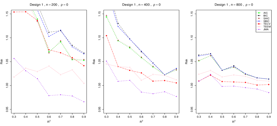
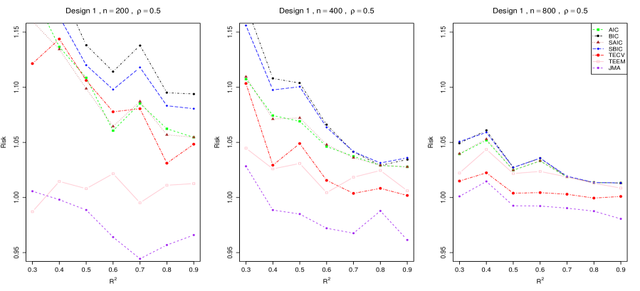
Figure 1: Results of simulations under Design 1

We set the sample size $n=200,400,800$ to compare all the methods to see the performance under finite sample cases and vary $R^{2}=0.3,0.4,0.5,...,0.9$. The results of simulation are presented in Appendix A. Figure 1 - 2 show that when for both design 1 and design 2, no matter $\rho$ equals to 0 or 0.5, our proposed estimator JMA performs best. Especially in the case of small samples, JMA has significant advantages over other methods. TEEM has the second best performance in the case of $n=200$ while TECV exceeds TEEM when $n$ becomes to 800. AIC, BIC, SAIC, SBIC do not perform well in all the cases. In other hand, when $R^{2}$ increases, the performance gap between JMA and other methods becomes large. Therefore, our proposed estimator has good performance in finite sample case in terms of average squared errors.

5.2 When there exist correct models

Then, we check the weight consistency of our method on the same model settings while in this case, we use four different candidate models as follows:

Table 2: Candidate models for the simulation study 2

Model	Candidate Model
1	$Y_{i}=[\beta_{1}u_{i1}^{2}+\beta_{2}u_{i2}+\beta_{3}u_{i1}+\beta_{4}u_{i2}^{2}+\zeta_{i}]I(T_{i}=1)+[\gamma_{1}u_{i1}^{2}+\gamma_{2}u_{i2}+v_{i}]I(T_{i}=0)$
2	$Y_{i}=[\beta_{3}u_{i3}+\zeta_{i}]I(T_{i}=1)+[\gamma_{3}u_{i3}+\nu_{i}]I(T_{i}=0)$
3	$Y_{i}=[\beta_{4}u_{i4}+\zeta_{i}]I(T_{i}=1)+[\gamma_{4}u_{i4}+\nu_{i}]I(T_{i}=0)$
4	$Y_{i}=[\beta_{0}+\zeta_{i}]I(T_{i}=1)+[\gamma_{0}+\nu_{i}]I(T_{i}=0)$

where only the first candidate model is correct. In the j-th replication, we record the weight assigned to the first model, which is the correct model as follows,

$$\hat{w}_{\Delta,j}=\hat{w}_{1}.$$

We replicate each model $J=100$ times and compute the average weight assigned to the correct model as

$$\hat{w}_{\Delta}=\frac{1}{J}\sum_{j=1}^{J}\hat{w}_{\Delta,j}.$$

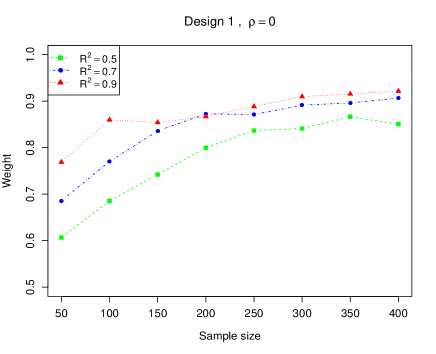
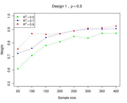
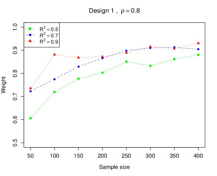
Figure 3: Sum of weights assigned to the correct models under Design 1.

The results of simulation are presented in Appendix B. From Figure 3 - 4 we can see that in all the settings, as the sample size increases, the weight assigned to the correct model also increases and becomes closer to 1. This result supports our theoretical result about weight consistency.

6 Empirical Application

In our empirical application, we consider the LaLonde, (1986) National Supported Work Demonstration data set. The NSW Demonstration provided work experience training to people who were struggling financially. Participants were randomly assigned to the treatment group or control group, which repreesnts that this person accepts training or not. Rolling et al., (2019) analyzed this data set, which focuses on the male participants, and we also focus on the male participants. The aim of this analysis is to estimate the treatment effects of work training on the outcome. The data set contains 722 observations, of which 297 are in the treatment group and 425 are in the control group. We consider the difference in the square root of income between 1975 (pre-treatment) and 1978 (post-treatment) as our response. The treatment variable $T$ equaling to 1 means this person accepted training in the NSW Demonstration and 0 otherwise. We use four baseline covariates (square root of 1975 income, age, years of education, marital status), which are all measured before the training to identify heterogeneous treatment effects, thus the estimation of conditional average treatment effects is our goal.

When we construct the candidate models, we take the interaction terms between the binary variable Married and other 3 continous variables and the quadratic terms of these 3 continous variables into account. The first four candidate models don’t contain the treatment variable thus they have no treatment effects. We add the treatment variable and vary the number of the baseline covariates from 1 to 4 to construct the additional 15 candidate models. In this way, we can get the marginal and combined effects of these covariates. Based on the 19-th candidate model, we add the interaction terms and the quadratic terms respectively to construct the additional 6 models, which consider the possible nonlinear relationship between the outcome and these covariates. We list all the covariates each candidate model uses in Table 3.

We evaluate the different estimators by a “guided simulation” experiment, that is, we need a “true” process to generate the response values so that we can obtain the “true” treatment effects to evaluate the estimators. We choose the 19-th model, the 5-th and 25-th model, which are selected by three model selection methods AIC, BIC, TECV respectively as the “true” processes. For each “true” process, we use this model to estimate error variance, which is denoted as $\hat{\sigma}^{2}$. Then for each replication, we generate random variables $u_{i}$ from $\text{Unif}(0.5,1.5)$, and use $u_{i}^{2}*\hat{\sigma}^{2}$ as the variance to generate a noise variable from zero-mean Gaussian distribution. Then we generate the same number of observations of $Y$ by augmenting the estimated regression using this “true” model with the noise variables. For each method, we can obtain the estimated treatment effects $\hat{\Delta}(\mathbf{u}_{i})$ and we evaluate the performance of the method by the average of the squared errors $(\Delta(\mathbf{u}_{i})-\hat{\Delta}(\mathbf{u}_{i}))^{2}$ across the 722 observations. In each replication, we can obtain the “true” treatment effects $\Delta(\mathbf{u}_{i})$ from the assumed true process. We repeat the experiment 100 times, and different realisations of the noises are generated for each trial.

The results are presented in the Appendix C, from which we can see that when we assume the 19-th candidate model as the “true” process, the JMA estimator has the best performance among all the methods, followed by the TEEM, SAIC, and other methods. JMA estimator also results in the smallest variance of average squared errors, which indicates that our method is robust for the heteroskedastic error settings. When we use the 5-th candidate model as the “true” process, the BIC and SBIC methods perform best since we choose the candidate model determined by BIC criterion as the “true” process. In this case, the JMA estimator still has a good performance. When we use the 25-th candidate model as the “true” process, the JMA estimator has the best performance with smallest variance of average squared errors. Therefore, our proposed method has a good performance in real data analysis in terms average squared errors and the estimator has small variance thus it is robust.

Table 3: Candidate models in the empirical example

Model	Covariates
1	Educ
2	Age, Educ
3	Married, Educ
4	Age, Married, Inc75, Educ
5	T, Inc75, T*Inc75
6	T, Age, T*Age
7	T, Educ, T*Educ
8	T, Married, T*Married
9	T, Inc75, T*Inc75, Age, T*Age
10	T, Inc75, T*Inc75, Educ, T*Educ
11	T, Inc75, T*Inc75, Married, T*Married
12	T, Age, T*Age, Educ, T*Educ
13	T, Age, T*Age, Married, T*Married
14	T, Educ, T*Educ, Married, T*Married
15	T, Inc75, T*Inc75, Age, T*Age, Educ, T*Educ
16	T, Inc75, T*Inc75, Age, T*Age, Married, T*Married
17	T, Inc75, T*Inc75, Educ, T*Educ, Married, T*Married
18	T, Age, T*Age, Married, T*Married, Educ, T*Educ
19	T, Age, T*Age, Married, T*Married, Educ, T*Educ, Inc75, T*Inc75
20	T, Age, T*Age, Married, T*Married, Educ, T*Educ, Inc75, T*Inc75, Age*Married
	Educ*Married, Inc75*Married, T*Age*Married
21	T, Age, T*Age, Married, T*Married, Educ, T*Educ, Inc75, T*Inc75, Age*Married
	Educ*Married, Inc75*Married, T*Age*Married, T*Educ*Married
22	T, Age, T*Age, Married, T*Married, Educ, T*Educ, Inc75, T*Inc75, Age*Married
	Educ*Married, Inc75*Married, T*Age*Married, T*Educ*Married, T*Inc75*Married
23	T, Age, T*Age, Married, T*Married, Educ, T*Educ, Inc75, T*Inc75 Age*Married
	Educ*Married, Inc75*Married, $\text{Age}^{2}$, $\text{T}*\text{Age}^{2}$
24	T, Age, T*Age, Married, T*Married, Educ, T*Educ, Inc75, T*Inc75 Age*Married
	Educ*Married, Inc75*Married, $\text{Educ}^{2}$, $\text{T}*\text{Educ}^{2}$
25	T, Age, T*Age, Married, T*Married, Educ, T*Educ, Inc75, T*Inc75 Age*Married
	Educ*Married, Inc75*Married, $\text{Inc75}^{2}$, $\text{T}*\text{Inc75}^{2}$

7 Conclusion

In this paper, we have proposed the jackknife model averaging estimator for the conditional average treatment effects under heteroskedastic error settings, and we also developed the theoretical properties of the proposed estimator. When all the candidate models are misspecified, Theorem 1 guarantees that our estimator achieves the lowest possible mean squared error as the sample size increases to infinity. When there exists correct candidate models, Theorem 2 guarantees that the weight assigned to the correct models converges to 1 as the sample size increases to infinity. A Monte Carlo simulation shows the proposed method has a good performance in finite samples. However, there still exist some extensions. First, we limit the covariate dimension, which can go to infinity only with a slower rate than the increasing rate of the sample size. Thus, how to extend this method to high dimensional data, where the covariate dimension exceeds the sample size is a good extension. Second, all the analysis in this paper is based on a linear model framework. Thus, extensions to non-linear model or non-parametric model are of importance.

Appendix A Results of simulation 1

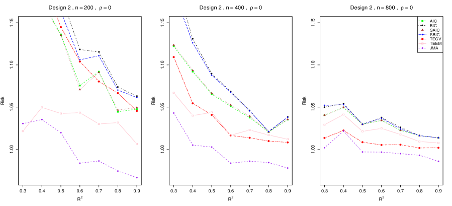
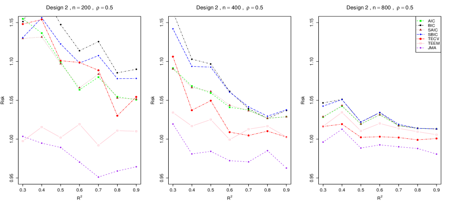
Figure 2: Results of simulations under Design 2

Appendix B Results of simulation 2

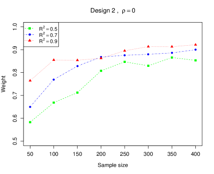
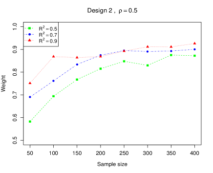
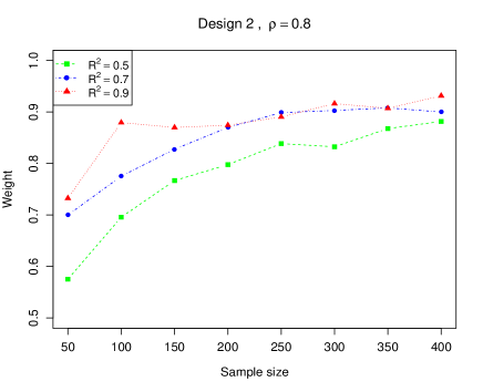
Figure 4: Sum of weights assigned to the correct models under Design 2.

Appendix C Results of real data analysis

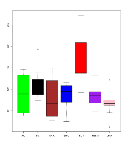
Figure 5: Box-plot of average squared errors in empirical application when we assume the 19-th candidate model, which is chosen by AIC as the “true” process.

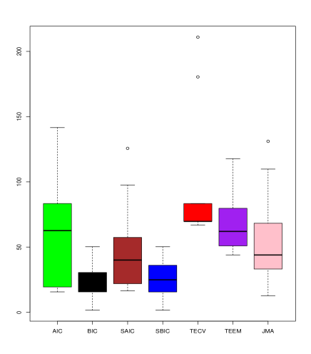
Figure 6: Box-plot of average squared errors in empirical application when we assume the 5-th candidate model, which is chosen by BIC as the “true” process.

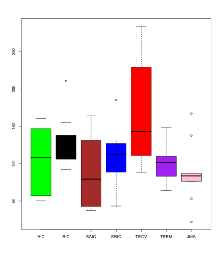
Figure 7: Box-plot of average squared errors in empirical application when we assume the 25-th candidate model, which is chosen by TECV as the “true” process.

Appendix D Proof of Theorem 1

Denote that $\operatorname*{Cov}(\boldsymbol{\zeta}_{t}\mid\operatorname*{\mathbf{u}})=\Omega_{1}$ and $\operatorname*{Cov}(\boldsymbol{\nu}_{c}\mid\operatorname*{\mathbf{u}})=\Omega_{2}$. Assume that $\vartheta(\Omega_{1}),\vartheta(\Omega_{2})\leq\bar{C}<\infty,$ almost sure, where $\bar{C}$ is a finite constant. Let $\tilde{\xi}_{n}=\inf_{\operatorname*{\mathbf{w}}\in Q_{n}}\tilde{R}_{n}(\operatorname*{\mathbf{w}})$. If $\sup_{\operatorname*{\mathbf{w}}\in Q_{n}}\bigg{|}\tilde{R}_{n}(\operatorname*{\mathbf{w}})/R_{n}(\operatorname*{\mathbf{w}})-1\bigg{|}\leq 1$, by Condition 4.1 and Condition 4.2, following the proof of (A.1) in Zhang et al. (2013), we have

$$K\tilde{\xi}_{n}^{-2G}\sum_{k=1}^{K}\{\tilde{R}_{n}(\mathbf{w}_{k}^{0})\}^{G}\stackrel{{\scriptstyle a.s.}}{{\longrightarrow}}0.$$ (D.1)

We next show that

$$\tilde{L}_{n}(\hat{\operatorname*{\mathbf{w}}})/\inf_{\operatorname*{\mathbf{w}}\in Q_{n}}\tilde{L}_{n}(\operatorname*{\mathbf{w}})\stackrel{{\scriptstyle p}}{{\longrightarrow}}1.$$ (D.2)

Observe that

$$\text{CV}_{n}(\operatorname*{\mathbf{w}}) =||\tilde{\operatorname*{\mathbf{Y}}}-\tilde{\Delta}(\operatorname*{\mathbf{w}})||^{2}$$

$$=2<\Delta+\operatorname*{\mathbf{b}}-\tilde{\Delta}(\operatorname*{\mathbf{w}}),\operatorname*{\boldsymbol{\eta}}>+||\Delta+\operatorname*{\mathbf{b}}-\tilde{\Delta}(\operatorname*{\mathbf{w}})||^{2}+||\operatorname*{\boldsymbol{\eta}}||^{2}$$

$$=\tilde{L}_{n}(\operatorname*{\mathbf{w}})+2<\Delta+\operatorname*{\mathbf{b}}-\tilde{\Delta}(\operatorname*{\mathbf{w}}),\operatorname*{\boldsymbol{\eta}}>+\underline{\tilde{L}}_{n}(\operatorname*{\mathbf{w}})-\tilde{L}_{n}(\operatorname*{\mathbf{w}})+||\operatorname*{\boldsymbol{\eta}}||^{2},$$ (D.3)

where $\underline{\tilde{L}}_{n}(\operatorname*{\mathbf{w}})=||\Delta+\operatorname*{\mathbf{b}}-\tilde{\Delta}(\operatorname*{\mathbf{w}})||^{2}$. Therefore, to prove (D.2), it sufficies to show that

$$\sup_{\operatorname*{\mathbf{w}}\in Q_{n}}\frac{|<\Delta+\operatorname*{\mathbf{b}}-\tilde{\Delta}(\operatorname*{\mathbf{w}}),\operatorname*{\boldsymbol{\eta}}>|}{\tilde{R}_{n}(\operatorname*{\mathbf{w}})}\stackrel{{\scriptstyle p}}{{\longrightarrow}}0,$$ (D.4)

$$\sup_{\operatorname*{\mathbf{w}}\in Q_{n}}\frac{|\underline{\tilde{L}}_{n}(\operatorname*{\mathbf{w}})-\tilde{L}_{n}(\operatorname*{\mathbf{w}})|}{\tilde{R}_{n}(\operatorname*{\mathbf{w}})}\stackrel{{\scriptstyle p}}{{\longrightarrow}}0,$$ (D.5)

$$\sup_{\operatorname*{\mathbf{w}}\in Q_{n}}\bigg{|}\frac{\tilde{L}_{n}(\operatorname*{\mathbf{w}})}{\tilde{R}_{n}(\operatorname*{\mathbf{w}})}-1\bigg{|}\stackrel{{\scriptstyle p}}{{\longrightarrow}}0.$$ (D.6)

We next prove (D.4). Since

$$<\Delta+\operatorname*{\mathbf{b}}-\tilde{\Delta}(\operatorname*{\mathbf{w}}),\operatorname*{\boldsymbol{\eta}}>$$

$$= <\mathbf{f}_{t}-\mathbf{f}_{c}-\tilde{P}_{t}(\operatorname*{\mathbf{w}})\mathbf{f}_{ta}+\tilde{P}_{c}(\operatorname*{\mathbf{w}})\mathbf{f}_{ca}-\tilde{P}_{t}(\operatorname*{\mathbf{w}})\boldsymbol{\zeta}_{ta}+\tilde{P}_{c}(\operatorname*{\mathbf{w}})\mathbf{v}_{ca},\operatorname*{\boldsymbol{\eta}}>$$

$$= <\mathbf{f}_{t}-\tilde{P}_{t}(\operatorname*{\mathbf{w}})\mathbf{f}_{ta},\operatorname*{\boldsymbol{\eta}}>-<\mathbf{f}_{c}-\tilde{P}_{c}(\operatorname*{\mathbf{w}})\mathbf{f}_{ca},\operatorname*{\boldsymbol{\eta}}>-<\tilde{P}_{t}(\operatorname*{\mathbf{w}})\boldsymbol{\zeta}_{ta},\operatorname*{\boldsymbol{\eta}}>+<\tilde{P}_{c}(\operatorname*{\mathbf{w}})\mathbf{v}_{ca},\operatorname*{\boldsymbol{\eta}}>$$

$$= <\tilde{A}_{t}(\operatorname*{\mathbf{w}}),\operatorname*{\boldsymbol{\eta}}>-<\tilde{A}_{c}(\operatorname*{\mathbf{w}}),\operatorname*{\boldsymbol{\eta}}>-<\tilde{P}_{t}(\operatorname*{\mathbf{w}})\boldsymbol{\zeta}_{ta},\operatorname*{\boldsymbol{\eta}}>+<\tilde{P}_{c}(\operatorname*{\mathbf{w}})\mathbf{v}_{ca},\operatorname*{\boldsymbol{\eta}}>$$

$$= <\tilde{A}_{t}(\operatorname*{\mathbf{w}}),\operatorname*{\boldsymbol{\eta}}>-<\tilde{A}_{c}(\operatorname*{\mathbf{w}}),\operatorname*{\boldsymbol{\eta}}>-[<\tilde{P}_{t}(\operatorname*{\mathbf{w}})\boldsymbol{\zeta}_{ta},\operatorname*{\boldsymbol{\eta}}>-tr\{\tilde{P}_{t0}(\operatorname*{\mathbf{w}})\Omega_{1}\}]+$$

$$[<\tilde{P}_{c}(\operatorname*{\mathbf{w}})\mathbf{v}_{ca},\operatorname*{\boldsymbol{\eta}}>-tr\{\tilde{P}_{c0}(\operatorname*{\mathbf{w}})\Omega_{2}\}]-tr\{\tilde{P}_{t0}(\operatorname*{\mathbf{w}})\Omega_{1}\}+tr\{\tilde{P}_{c0}(\operatorname*{\mathbf{w}})\Omega_{2}\},$$ (D.7)

by Condition 4.3, Condition 4.4, and Lemma 3.1 in Ando Li (2014), we have

$$tr\{\tilde{P}_{t}(\mathbf{w}_{k}^{0})\tilde{P}_{t}(\mathbf{w}_{k}^{0})^{T}\}\leq\left[\frac{1}{1-\bar{\lambda}\{P_{t}(\mathbf{w}_{k}^{0})\}}\right]^{2}p_{k}\leq C\cdot p_{k},$$ (D.8)

where $\bar{\lambda}\{P_{t}(\mathbf{w}_{k}^{0})\}$ is the maximal diagonal element of $P_{t}(\mathbf{w}_{k}^{0})$. Then

$$\sup_{\operatorname*{\mathbf{w}}\in Q_{n}}\bigg{|}\frac{tr\{\tilde{P}_{t}(\operatorname*{\mathbf{w}})\tilde{\Omega}_{1}\}}{\tilde{R}_{n}}\bigg{|}$$

$$\leq \sum_{k=1}^{K}\bigg{|}\frac{tr\{\tilde{P}_{t}(\mathbf{w}_{k}^{0})\tilde{\Omega}_{1}\}}{\inf_{\operatorname*{\mathbf{w}}\in Q_{n}}\tilde{R}_{n}}\bigg{|}$$

$$\leq \sum_{k=1}^{K}\bigg{|}\frac{\sqrt{tr\{\tilde{P}_{t}(\mathbf{w}_{k}^{0})\tilde{P}_{t}(\mathbf{w}_{k}^{0})^{T}\}\cdot tr(\tilde{\Omega}_{1}\tilde{\Omega}_{1}^{T})}}{\inf_{\operatorname*{\mathbf{w}}\in Q_{n}}\tilde{R}_{n}}\bigg{|}$$

$$\leq \sum_{k=1}^{K}\bigg{|}\frac{\sqrt{C_{1}\cdot p_{k}\cdot C_{2}\cdot n}}{\inf_{\operatorname*{\mathbf{w}}\in Q_{n}}\tilde{R}_{n}}\bigg{|}$$

$$\leq \frac{C\cdot K\cdot p^{1/2}\cdot n^{1/2}}{\tilde{\xi}_{n}}\rightarrow 0,$$ (D.9)

where $K$ is the number of candidate models, $p$ is the number of covariates, and $n$ is the sample size. Therefore, to prove (D.4), it sufficies to show that

$$\sup_{\operatorname*{\mathbf{w}}\in Q_{n}}|<\tilde{A}_{t}(\operatorname*{\mathbf{w}}),\operatorname*{\boldsymbol{\eta}}>|/\tilde{R}_{n}(\operatorname*{\mathbf{w}})\stackrel{{\scriptstyle p}}{{\longrightarrow}}0,$$ (D.10)

$$\sup_{\operatorname*{\mathbf{w}}\in Q_{n}}|<\tilde{A}_{c}(\operatorname*{\mathbf{w}}),\operatorname*{\boldsymbol{\eta}}>|/\tilde{R}_{n}(\operatorname*{\mathbf{w}})\stackrel{{\scriptstyle p}}{{\longrightarrow}}0,$$ (D.11)

$$\sup_{\operatorname*{\mathbf{w}}\in Q_{n}}\frac{|<\tilde{P}_{t}(\operatorname*{\mathbf{w}})\operatorname*{\boldsymbol{\zeta}}_{ta},\operatorname*{\boldsymbol{\eta}}>-tr\{\tilde{P}_{t0}(\operatorname*{\mathbf{w}})\Omega_{1}\}|}{\tilde{R}_{n}(\operatorname*{\mathbf{w}})}\stackrel{{\scriptstyle p}}{{\longrightarrow}}0,$$ (D.12)

$$\sup_{\operatorname*{\mathbf{w}}\in Q_{n}}\frac{|<\tilde{P}_{c}(\operatorname*{\mathbf{w}})\mathbf{v}_{ca},\operatorname*{\boldsymbol{\eta}}>-tr\{\tilde{P}_{c0}(\operatorname*{\mathbf{w}})\Omega_{2}\}|}{\tilde{R}_{n}(\operatorname*{\mathbf{w}})}\stackrel{{\scriptstyle p}}{{\longrightarrow}}0.$$ (D.13)

To prove (D.10), using Chebyshev’s inequality and Theorem 2 of Whittle (1960), and following steps similar to the proof of (A.1) in Wan et al. (2010), we have that for any $\delta>0$,

$$\operatorname*{Pr}\biggl{\{}\sup_{\operatorname*{\mathbf{w}}\in Q_{n}}\frac{|<\tilde{A}_{t}(\operatorname*{\mathbf{w}}),\operatorname*{\boldsymbol{\eta}}>|}{\tilde{R}_{n}(\operatorname*{\mathbf{w}})}>\delta\biggl{\}}$$

$$\leq \operatorname*{Pr}\biggl{\{}\sup_{\operatorname*{\mathbf{w}}\in Q_{n}}\sum_{k=1}^{K}\mathbf{w}_{k}|\boldsymbol{\eta}^{T}(\mathbf{f}_{t}-\tilde{P}_{t}^{(k)}\mathbf{f}_{ta})|>\delta\tilde{\xi}_{n}\biggl{\}}$$

$$\leq \operatorname*{Pr}\biggl{\{}\max_{1\leq k\leq K}|\boldsymbol{\eta}^{T}(\mathbf{f}_{t}-\tilde{P}_{t}^{(k)}\mathbf{f}_{ta})|>\delta\tilde{\xi}_{n}\biggl{\}}$$

$$= \operatorname*{Pr}\biggl{[}\{|<\operatorname*{\boldsymbol{\eta}},\tilde{A}_{t}(\mathbf{w}_{1}^{0})>|>\delta\tilde{\xi}_{n}\}\cup...\cup\{|<\operatorname*{\boldsymbol{\eta}},\tilde{A}_{t}(\mathbf{w}_{K}^{0})>|>\delta\tilde{\xi}_{n}\}\biggl{]}$$

$$\leq \sum_{k=1}^{K}\operatorname*{Pr}\{|<\operatorname*{\boldsymbol{\eta}},\tilde{A}_{t}(\mathbf{w}_{1}^{0})>|>\delta\tilde{\xi}_{n}\}$$

$$\leq \sum_{k=1}^{K}\operatorname*{Pr}\{|<\boldsymbol{\zeta}_{t},\tilde{A}_{t}(\mathbf{w}_{1}^{0})>|+|<\mathbf{v}_{c},\tilde{A}_{t}(\mathbf{w}_{1}^{0})>|>\delta\tilde{\xi}_{n}\}$$

$$\leq \sum_{k=1}^{K}\operatorname*{Pr}\{|<\boldsymbol{\zeta}_{t},\tilde{A}_{t}(\mathbf{w}_{1}^{0})>|>\frac{1}{2}\delta\tilde{\xi}_{n}\}+\operatorname*{Pr}\{|<\mathbf{v}_{c},\tilde{A}_{t}(\mathbf{w}_{1}^{0})>|>\frac{1}{2}\delta\tilde{\xi}_{n}\}$$

$$\leq C_{1}\delta^{-2G}\tilde{\xi}_{n}^{-2G}\sum_{k=1}^{K}\operatorname*{E}\{\boldsymbol{\zeta}_{t}^{T}\tilde{A}_{t}(\mathbf{w}_{k}^{0})\}^{2G}+\operatorname*{E}\{\mathbf{v}_{c}^{T}\tilde{A}_{t}(\mathbf{w}_{k}^{0})\}^{2G}$$

$$\leq C_{1}\delta^{-2G}\tilde{\xi}_{n}^{-2G}\sum_{k=1}^{K}||\Omega_{1}^{\frac{1}{2}}\tilde{A}_{t}(\mathbf{w}_{k}^{0})||^{2G}+||\Omega_{2}^{\frac{1}{2}}\tilde{A}_{t}(\mathbf{w}_{k}^{0})||^{2G}$$

$$\leq C_{1}\delta^{-2G}\tilde{\xi}_{n}^{-2G}[\{\vartheta^{G}(\Omega_{1})+\vartheta^{G}(\Omega_{2})\}\sum_{k=1}^{K}]||\tilde{A}_{t}(\mathbf{w}_{k}^{0})||^{2G}]\rightarrow 0.$$ (D.14)

Hence (D.10) has been proved and similarly (D.11) is also valid. For any $\delta>0$, we have that

$$\operatorname*{Pr}\bigg{\{}\sup_{\operatorname*{\mathbf{w}}\in Q_{n}}\frac{|<\tilde{P}_{t}(\operatorname*{\mathbf{w}})\operatorname*{\boldsymbol{\zeta}}_{ta},\operatorname*{\boldsymbol{\eta}}>-tr(\tilde{P}_{t0}(\operatorname*{\mathbf{w}})\Omega_{1})|}{\tilde{R}_{n}(\operatorname*{\mathbf{w}})}>\delta\bigg{\}}$$

$$\leq \operatorname*{Pr}\bigg{\{}\sup_{\operatorname*{\mathbf{w}}\in Q_{n}}\frac{|<\tilde{P}_{t}(\operatorname*{\mathbf{w}})\operatorname*{\boldsymbol{\zeta}}_{ta},\boldsymbol{\zeta}_{t}>-tr(\tilde{P}_{t0}(\operatorname*{\mathbf{w}})\Omega_{1})|}{\tilde{R}_{n}(\operatorname*{\mathbf{w}})}>\delta\bigg{\}}+$$

$$\operatorname*{Pr}\bigg{\{}\sup_{\operatorname*{\mathbf{w}}\in Q_{n}}\frac{|<\tilde{P}_{t}(\operatorname*{\mathbf{w}})\operatorname*{\boldsymbol{\zeta}}_{ta},\mathbf{v}_{c}>|}{\tilde{R}_{n}(\operatorname*{\mathbf{w}})}>\delta\bigg{\}},$$ (D.15)

and

$$\operatorname*{Pr}\bigg{\{}\sup_{\operatorname*{\mathbf{w}}\in Q_{n}}\frac{|<\tilde{P}_{t}(\operatorname*{\mathbf{w}})\operatorname*{\boldsymbol{\zeta}}_{ta},\boldsymbol{\zeta}_{t}>-tr(\tilde{P}_{t0}(\operatorname*{\mathbf{w}})\Omega_{1})|}{\tilde{R}_{n}(\operatorname*{\mathbf{w}})}>\delta\bigg{\}}$$

$$\leq \sum_{k=1}^{K}\operatorname*{Pr}\bigg{[}|<\tilde{P}_{t}(\mathbf{w}_{k}^{0}\boldsymbol{\zeta}_{ta}),\boldsymbol{\zeta}_{t}>-tr\{\tilde{P}_{t0}(\operatorname*{\mathbf{w}})\Omega_{1}\}|>\delta\tilde{\xi}_{n}\bigg{]}$$

$$\leq \sum_{k=1}^{K}\operatorname*{Pr}\bigg{[}|<\tilde{P}_{t0}(\mathbf{w}_{k}^{0}\boldsymbol{\zeta}_{ta}),\boldsymbol{\zeta}_{t}>-tr\{\tilde{P}_{t0}(\operatorname*{\mathbf{w}})\Omega_{1}\}|>\delta\tilde{\xi}_{n}\bigg{]}$$

$$\leq \operatorname*{E}\biggl{(}\frac{[<\tilde{P}_{t0}(\mathbf{w}_{k}^{0}\boldsymbol{\zeta}_{ta}),\boldsymbol{\zeta}_{t}>-tr\{\tilde{P}_{t0}(\operatorname*{\mathbf{w}})\Omega_{1}\}]^{2G}}{\delta^{2G}\tilde{\xi}_{n}^{2G}}\biggl{)}$$

$$\leq C_{2}\delta^{-2G}\tilde{\xi}_{n}^{-2G}\sum_{k=1}^{K}[tr\{\tilde{P}_{t0}(\mathbf{w}_{k}^{0})\tilde{P}_{t0}^{\prime}(\mathbf{w}_{k}^{0})\}]^{G}$$

$$= C_{2}\delta^{-2G}\tilde{\xi}_{n}^{-2G}\sum_{k=1}^{K}[tr\{\tilde{P}_{t}(\mathbf{w}_{k}^{0})\tilde{P}_{t}^{\prime}(\mathbf{w}_{k}^{0})\}]^{G}\rightarrow 0,$$ (D.16)

and

$$\operatorname*{Pr}\bigg{\{}\sup_{\operatorname*{\mathbf{w}}\in Q_{n}}\frac{|<\tilde{P}_{t}(\operatorname*{\mathbf{w}})\operatorname*{\boldsymbol{\zeta}}_{ta},\mathbf{v}_{c}>|}{\tilde{R}_{n}(\operatorname*{\mathbf{w}})}>\delta\bigg{\}}$$

$$\leq \sum_{k=1}^{K}\operatorname*{Pr}\bigg{[}|<\tilde{P}_{t}(\mathbf{w}_{k}^{0})\boldsymbol{\zeta}_{ta},\mathbf{v}_{c}>-\operatorname*{E}\{<\tilde{P}_{t}(\mathbf{w}_{k}^{0})\boldsymbol{\zeta}_{ta},\mathbf{v}_{c}>\}|>\delta\tilde{\xi}_{n}\bigg{]}$$

$$= \sum_{k=1}^{K}\operatorname*{Pr}\bigg{\{}|<\tilde{P}_{t}(\mathbf{w}_{k}^{0})\boldsymbol{\zeta}_{ta},\mathbf{v}_{ca}>|>\delta\tilde{\xi}_{n}\bigg{\}}$$

$$\leq \sum_{k=1}^{K}\operatorname*{E}\bigg{[}\frac{\{<\tilde{P}_{t}(\mathbf{w}_{k}^{0})\operatorname*{\boldsymbol{\zeta}}_{ta},\mathbf{v}_{c}>\}^{2}}{\delta^{2}\tilde{\xi}_{n}^{2}}\bigg{]}$$

$$\leq \sum_{k=1}^{K}\operatorname*{E}\bigg{\{}\frac{\boldsymbol{\zeta}_{ta}^{\prime}\tilde{P}_{t}^{\prime}(\mathbf{w}_{k}^{0})\mathbf{v}_{c}\mathbf{v}_{c}^{\prime}\tilde{P}_{t}(\mathbf{w}_{k}^{0})\boldsymbol{\zeta}_{ta}}{\delta^{2}\tilde{\xi}_{n}^{2}}\bigg{\}}$$

$$\leq C_{3}\delta^{-2}\tilde{\xi}_{n}^{-2}\sum_{k=1}^{K}tr\{\tilde{P}_{t}(\mathbf{w}_{k}^{0})\tilde{P}_{t}^{\prime}(\mathbf{w}_{k}^{0})\}\rightarrow 0.$$ (D.17)

Hence (D.12) has been proved and similarly (D.13) is also valid. Thus (D.4) has been proved. Then we prove (D.5). Let $\underline{\tilde{R}}_{n}(\operatorname*{\mathbf{w}})=\operatorname*{E}(\underline{\tilde{L}}_{n}(\operatorname*{\mathbf{w}})\mid\mathbf{u})$. Similar to the proof of (A.24) in Zhao et al. (2021), we obtain that

$$\sup_{\operatorname*{\mathbf{w}}\in Q_{n}}|\underline{\tilde{R}}_{n}(\operatorname*{\mathbf{w}})-\tilde{R}_{n}(\operatorname*{\mathbf{w}})|/\tilde{R}_{n}(\operatorname*{\mathbf{w}})$$

$$= \sup_{\operatorname*{\mathbf{w}}\in Q_{n}}\operatorname*{E}[\{||\Delta+\operatorname*{\mathbf{b}}-\tilde{\Delta}(\operatorname*{\mathbf{w}})||^{2}-||\Delta-\tilde{\Delta}(\operatorname*{\mathbf{w}})||^{2}\}\mid\mathbf{u}]/\tilde{R}_{n}(\operatorname*{\mathbf{w}})$$

$$= \sup_{\operatorname*{\mathbf{w}}\in Q_{n}}\operatorname*{E}\{2<\Delta-\tilde{\Delta}(\operatorname*{\mathbf{w}}),\operatorname*{\mathbf{b}}>+||\operatorname*{\mathbf{b}}||^{2}\mid\mathbf{u}\}/\tilde{R}_{n}(\operatorname*{\mathbf{w}})$$

$$= o(1).$$ (D.18)

Similar to the proof of (A.25) in Zhao et al. (2021), we obtain that

$$\sup_{\operatorname*{\mathbf{w}}\in Q_{n}}\underline{\tilde{L}}_{n}(\operatorname*{\mathbf{w}})/\tilde{R}_{n}(\operatorname*{\mathbf{w}})-1$$

$$= \sup_{\operatorname*{\mathbf{w}}\in Q_{n}}[\{\underline{\tilde{L}}_{n}(\operatorname*{\mathbf{w}})-\underline{\tilde{R}}_{n}(\operatorname*{\mathbf{w}})\}+\{\underline{\tilde{R}}_{n}(\operatorname*{\mathbf{w}})-\tilde{R}_{n}(\operatorname*{\mathbf{w}})\}]/\tilde{R}_{n}(\operatorname*{\mathbf{w}})\stackrel{{\scriptstyle p}}{{\longrightarrow}}0.$$ (D.19)

Similar to the proof of (A.26) in Zhao et al. (2021), we obtain that

$$\sup_{\operatorname*{\mathbf{w}}\in Q_{n}}|\underline{\tilde{L}}_{n}(\operatorname*{\mathbf{w}})-\tilde{L}_{n}(\operatorname*{\mathbf{w}})|/\tilde{R}_{n}(\operatorname*{\mathbf{w}})$$

$$= \sup_{\operatorname*{\mathbf{w}}\in Q_{n}}\bigg{|}||\Delta+\operatorname*{\mathbf{b}}-\tilde{\Delta}(\operatorname*{\mathbf{w}})||^{2}-||\Delta-\tilde{\Delta}(\operatorname*{\mathbf{w}})||^{2}\bigg{|}/\tilde{R}_{n}(\operatorname*{\mathbf{w}})$$

$$\leq \sup_{\operatorname*{\mathbf{w}}\in Q_{n}}[2\{\underline{\tilde{L}}_{n}(\operatorname*{\mathbf{w}})||\operatorname*{\mathbf{b}}||\}^{1/2}]/\tilde{R}_{n}(\operatorname*{\mathbf{w}})+\sup_{\operatorname*{\mathbf{w}}\in Q_{n}}||\operatorname*{\mathbf{b}}||^{2}/\tilde{R}_{n}(\operatorname*{\mathbf{w}})\stackrel{{\scriptstyle p}}{{\longrightarrow}}0,$$ (D.20)

thus (D.5) is valid. Since

$$\sup_{\operatorname*{\mathbf{w}}\in Q_{n}}|\tilde{L}_{n}(\operatorname*{\mathbf{w}})/\tilde{R}_{n}(\operatorname*{\mathbf{w}})-1|$$

$$= \sup_{\operatorname*{\mathbf{w}}\in Q_{n}}|\{\underline{\tilde{L}}_{n}(\operatorname*{\mathbf{w}})-\tilde{L}_{n}(\operatorname*{\mathbf{w}})\}-\{\underline{\tilde{L}}_{n}(\operatorname*{\mathbf{w}})-\tilde{R}_{n}(\operatorname*{\mathbf{w}})\}|/\tilde{R}_{n}(\operatorname*{\mathbf{w}})$$

$$= \sup_{\operatorname*{\mathbf{w}}\in Q_{n}}|\underline{\tilde{L}}_{n}(\operatorname*{\mathbf{w}})-\tilde{L}_{n}(\operatorname*{\mathbf{w}})|/\tilde{R}_{n}(\operatorname*{\mathbf{w}})+\sup_{\operatorname*{\mathbf{w}}\in Q_{n}}|\underline{\tilde{L}}_{n}(\operatorname*{\mathbf{w}})-\tilde{R}_{n}(\operatorname*{\mathbf{w}})|/\tilde{R}_{n}(\operatorname*{\mathbf{w}})\stackrel{{\scriptstyle p}}{{\longrightarrow}}0,$$ (D.21)

(D.6) is valid, hence (D.2) is valid. Using the techinique in deriving (D.6), we have

$$\sup_{\operatorname*{\mathbf{w}}\in Q_{n}}|L_{n}(\operatorname*{\mathbf{w}})/R_{n}(\operatorname*{\mathbf{w}})-1|\stackrel{{\scriptstyle p}}{{\longrightarrow}}0.$$ (D.22)

Now upon using (D.2), (D.6) and (D.22) in

$$\frac{L_{n}(\hat{\operatorname*{\mathbf{w}}})}{\inf_{\operatorname*{\mathbf{w}}\in Q_{n}}L_{n}(\operatorname*{\mathbf{w}})}-1= \sup_{\operatorname*{\mathbf{w}}\in Q_{n}}\bigg{\{}\frac{L_{n}(\hat{\operatorname*{\mathbf{w}}})}{L_{n}(\operatorname*{\mathbf{w}})}-1\bigg{\}}$$

$$\leq \sup_{\operatorname*{\mathbf{w}}\in Q_{n}}\bigg{\{}\frac{L_{n}(\operatorname*{\mathbf{w}})}{R_{n}(\operatorname*{\mathbf{w}})}\bigg{\}}\sup_{\operatorname*{\mathbf{w}}\in Q_{n}}\bigg{\{}\frac{R_{n}(\operatorname*{\mathbf{w}})}{L_{n}(\operatorname*{\mathbf{w}})}\bigg{\}}\sup_{\operatorname*{\mathbf{w}}\in Q_{n}}\bigg{\{}\frac{\tilde{R}_{n}(\operatorname*{\mathbf{w}})}{R_{n}(\operatorname*{\mathbf{w}})}\bigg{\}}\sup_{\operatorname*{\mathbf{w}}\in Q_{n}}\bigg{\{}\frac{R_{n}(\operatorname*{\mathbf{w}})}{\tilde{R}_{n}(\operatorname*{\mathbf{w}})}\bigg{\}}$$

$$\sup_{\operatorname*{\mathbf{w}}\in Q_{n}}\bigg{\{}\frac{\tilde{R}_{n}(\operatorname*{\mathbf{w}})}{\tilde{L}_{n}(\operatorname*{\mathbf{w}})}\bigg{\}}\sup_{\operatorname*{\mathbf{w}}\in Q_{n}}\bigg{\{}\frac{\tilde{L}_{n}(\operatorname*{\mathbf{w}})}{\tilde{R}_{n}(\operatorname*{\mathbf{w}})}\bigg{\}}\frac{\tilde{L}_{n}(\hat{\operatorname*{\mathbf{w}}})}{\inf_{\operatorname*{\mathbf{w}}\in Q_{n}}\tilde{L}_{n}(\operatorname*{\mathbf{w}})}-1\stackrel{{\scriptstyle p}}{{\longrightarrow}}0,$$ (D.23)

Theorem 1 has been proved.

Appendix E Proof of Theorem 2

Write $\operatorname*{\mathbf{w}}^{0}=(w_{1}^{0},...,w_{k_{0}}^{0},0,...,0)^{T}\in Q_{n}$, that is $w_{k}^{0}\in[0,1]$ for $k=1,...,k_{0}$ and $\sum_{k=1}^{k_{0}}w_{k}^{0}=1$. Note that

$$CV(\mathbf{w}^{0}) =||\tilde{\boldsymbol{\Delta}}(\mathbf{w}^{0})-\tilde{\operatorname*{\mathbf{Y}}}||^{2}$$

$$=||\sum_{k=1}^{k_{0}}w_{k}^{0}\tilde{\boldsymbol{\Delta}}^{k}-\boldsymbol{\Delta}-(\operatorname*{\mathbf{b}}+\operatorname*{\boldsymbol{\eta}})||^{2}$$

$$=||\sum_{k=1}^{k_{0}}w_{k}^{0}\mathbf{U}_{t}(\tilde{\boldsymbol{\beta}}^{k}-\tilde{\boldsymbol{\gamma}}^{k}-\boldsymbol{\beta}+\boldsymbol{\gamma})-(\operatorname*{\mathbf{b}}+\operatorname*{\boldsymbol{\eta}})||2$$

$$=||\sum_{k=1}^{k_{0}}w_{k}^{0}\mathbf{U}_{t}(\tilde{\boldsymbol{\beta}}^{k}-\tilde{\boldsymbol{\gamma}}^{k}-\boldsymbol{\beta}+\boldsymbol{\gamma})||^{2}+||\operatorname*{\mathbf{b}}+\operatorname*{\boldsymbol{\eta}}||^{2}-$$

$$~{}~{}~{}2(\operatorname*{\mathbf{b}}+\operatorname*{\boldsymbol{\eta}})^{T}\bigg{\{}\sum_{k=1}^{k_{0}}w_{k}^{0}\mathbf{U}_{t}(\tilde{\boldsymbol{\beta}}^{k}-\tilde{\boldsymbol{\gamma}}^{k}-\boldsymbol{\beta}+\boldsymbol{\gamma})\bigg{\}}$$

$$\overset{\Delta}{=}||\sum_{k=1}^{k_{0}}w_{k}^{0}\mathbf{U}_{t}(\tilde{\boldsymbol{\beta}}^{k}-\tilde{\boldsymbol{\gamma}}^{k}-\boldsymbol{\beta}+\boldsymbol{\gamma})||^{2}+||\operatorname*{\mathbf{b}}+\operatorname*{\boldsymbol{\eta}}||^{2}-2\Psi_{1},$$ (E.1)

and

$$CV(\hat{\operatorname*{\mathbf{w}}}) =||\tilde{\boldsymbol{\Delta}}(\hat{\operatorname*{\mathbf{w}}})-\tilde{\operatorname*{\mathbf{Y}}}||^{2}$$

$$=||\boldsymbol{\Delta}^{*}(\hat{\operatorname*{\mathbf{w}}})-\boldsymbol{\Delta}+\tilde{\boldsymbol{\Delta}}(\hat{\operatorname*{\mathbf{w}}})-\boldsymbol{\Delta}^{*}(\hat{\operatorname*{\mathbf{w}}})-(\operatorname*{\mathbf{b}}+\operatorname*{\boldsymbol{\eta}})||^{2}$$

$$=||\boldsymbol{\Delta}^{*}(\hat{\operatorname*{\mathbf{w}}})-\boldsymbol{\Delta}||^{2}+||\tilde{\boldsymbol{\Delta}}(\hat{\operatorname*{\mathbf{w}}})-\boldsymbol{\Delta}^{*}(\hat{\operatorname*{\mathbf{w}}})||^{2}+||\operatorname*{\mathbf{b}}+\operatorname*{\boldsymbol{\eta}}||^{2}+$$

$$~{}~{}~{}2\{\boldsymbol{\Delta}^{*}(\hat{\operatorname*{\mathbf{w}}})-\boldsymbol{\Delta}\}^{T}\{\tilde{\boldsymbol{\Delta}}(\hat{\operatorname*{\mathbf{w}}})-\boldsymbol{\Delta}^{*}(\hat{\operatorname*{\mathbf{w}}})\}-$$

$$~{}~{}~{}2(\operatorname*{\mathbf{b}}+\operatorname*{\boldsymbol{\eta}})^{T}\boldsymbol{\Delta}^{*}(\hat{\operatorname*{\mathbf{w}}})+2(\operatorname*{\mathbf{b}}+\operatorname*{\boldsymbol{\eta}})^{T}\boldsymbol{\Delta}-2(\operatorname*{\mathbf{b}}+\operatorname*{\boldsymbol{\eta}})^{T}\{\tilde{\boldsymbol{\Delta}}(\hat{\operatorname*{\mathbf{w}}})-\boldsymbol{\Delta}^{*}(\hat{\operatorname*{\mathbf{w}}})\}$$

$$\overset{\boldsymbol{\Delta}}{=}L^{*}(\hat{\operatorname*{\mathbf{w}}})+||\tilde{\boldsymbol{\Delta}}(\hat{\operatorname*{\mathbf{w}}})-\boldsymbol{\Delta}^{*}(\hat{\operatorname*{\mathbf{w}}})||^{2}+||\operatorname*{\mathbf{b}}+\operatorname*{\boldsymbol{\eta}}||^{2}+2\Psi_{2}-2\Psi_{3}+2\Psi_{4}-2\Psi_{5}.$$ (E.2)

We then check the order of each term in $CV(\mathbf{w}^{0})$ and $CV(\hat{\operatorname*{\mathbf{w}}})$. Firstly since $\sup_{1\leq i\leq n}|b_{i}|=O\bigg{\{}p\left(\frac{\log n}{n}\right)^{1/p}\bigg{\}}=O(1)$, we have that

$$||\operatorname*{\mathbf{b}}+\operatorname*{\boldsymbol{\eta}}||^{2}=||\operatorname*{\mathbf{b}}||^{2}+||\operatorname*{\boldsymbol{\eta}}||^{2}+2\mathbf{b}^{T}\operatorname*{\boldsymbol{\eta}}=O(n)+O_{p}(n)+O_{p}(n)=O_{p}(n).$$ (E.3)

Denote $\operatorname*{\mathbf{w}}_{T}^{0}=(w_{1}^{0},...,w_{k_{0}}^{0})^{T}$, which is a subvector of $\operatorname*{\mathbf{w}}^{0}$, and $\Phi=\{(\tilde{\boldsymbol{\beta}}^{1}-\tilde{\boldsymbol{\gamma}}^{1}-\boldsymbol{\beta}+\boldsymbol{\gamma})^{T},...,(\tilde{\boldsymbol{\beta}}^{k_{0}}-\tilde{\boldsymbol{\gamma}}^{k_{0}}-\boldsymbol{\beta}+\boldsymbol{\gamma})^{T}\}$. By Condition 4.6, Condition 4.7 and recognising that in the correct models, $\tilde{\boldsymbol{\beta}}^{k}-\boldsymbol{\beta}=O_{p}(n^{-1/2})$ and $\tilde{\boldsymbol{\gamma}}^{k}-\boldsymbol{\gamma}=O_{p}(n^{-1/2})$, we have that

$$||\sum_{k=1}^{k_{0}}w_{k}^{0}\mathbf{U}_{t}(\tilde{\boldsymbol{\beta}}^{k}-\tilde{\boldsymbol{\gamma}}^{k}-\boldsymbol{\beta}+\boldsymbol{\gamma})||^{2}$$

$$= \mathbf{w}_{T}^{0T}\Phi\mathbf{U}_{t}^{T}\mathbf{U}_{t}\Phi^{T}\mathbf{w}_{T}^{0}$$

$$\leq \vartheta(\mathbf{U}_{t}^{T}\mathbf{U}_{t})\vartheta(\Phi\Phi^{T})\mathbf{w}_{T}^{0T}\mathbf{w}_{T}^{0}$$

$$= \vartheta(\mathbf{U}_{t}^{T}\mathbf{U}_{t})\sum_{k=1}^{k_{0}}||\tilde{\boldsymbol{\beta}}^{k}-\tilde{\boldsymbol{\gamma}}^{k}-\boldsymbol{\beta}+\boldsymbol{\gamma}||^{2}\mathbf{w}_{T}^{0T}\mathbf{w}_{T}^{0}$$

$$= O_{p}(n)\cdot k_{0}\cdot O_{p}(n^{-1/2})^{2}$$

$$= O_{p}(1).$$ (E.4)

Thus by (E.3) and (E), we have that

$$|\Psi_{1}| =|(\operatorname*{\mathbf{b}}+\operatorname*{\boldsymbol{\eta}})^{T}\sum_{k=1}^{k_{0}}w_{k}^{0}\mathbf{U}_{t}(\tilde{\boldsymbol{\beta}}^{k}-\tilde{\boldsymbol{\gamma}}^{k}-\boldsymbol{\beta}+\boldsymbol{\gamma})|$$

$$\leq||\operatorname*{\mathbf{b}}+\operatorname*{\boldsymbol{\eta}}||\cdot||\sum_{k=1}^{k_{0}}w_{k}^{0}\mathbf{U}_{t}(\tilde{\boldsymbol{\beta}}^{k}-\tilde{\boldsymbol{\gamma}}^{k}-\boldsymbol{\beta}+\boldsymbol{\gamma})||$$

$$=O_{p}(n^{1/2})O_{p}(1)$$

$$=O_{p}(n^{1/2}).$$ (E.5)

Therefore we have obtained the order of each term in $CV(\mathbf{w}^{0})$. Since $\boldsymbol{\beta}^{k^{*}}=\boldsymbol{\beta}$, $\boldsymbol{\gamma}^{k^{*}}=\boldsymbol{\gamma}$ for $k=1,...,k_{0}$, when the candidate model is a correct model, we can obtain that $\boldsymbol{\Delta}^{k^{*}}=\boldsymbol{\Delta}$. Then

$$L^{*}(\hat{\operatorname*{\mathbf{w}}})= ||\boldsymbol{\Delta}^{*}(\hat{\operatorname*{\mathbf{w}}})-\boldsymbol{\Delta}||^{2}$$

$$= ||\sum_{k=1}^{K}\hat{w}_{k}\boldsymbol{\Delta}^{k^{*}}-\boldsymbol{\Delta}||^{2}$$

$$= ||\sum_{k=1}^{k_{0}}\hat{w}_{k}\boldsymbol{\Delta}^{k^{*}}+\sum_{k=k_{0}+1}^{K}\hat{w}_{k}\boldsymbol{\Delta}^{k^{*}}-\boldsymbol{\Delta}||^{2}$$

$$= ||\hat{w}_{\Delta}\sum_{k=1}^{k_{0}}\frac{\hat{w}_{k}}{\hat{w}_{\Delta}}(\boldsymbol{\Delta}^{k^{*}}-\boldsymbol{\Delta})+(1-\hat{w}_{\Delta})\sum_{k=k_{0}+1}^{K}\frac{\hat{w}_{k}}{1-\hat{w}_{\Delta}}(\boldsymbol{\Delta}^{k^{*}}-\boldsymbol{\Delta})||^{2}$$

$$= (1-\hat{w}_{\Delta})^{2}||\sum_{k=k_{0}+1}^{K}\frac{\hat{w}_{k}}{1-\hat{w}_{\Delta}}(\boldsymbol{\Delta}^{k^{*}}-\boldsymbol{\Delta})||^{2}$$

$$= (1-\hat{w}_{\Delta})^{2}||\boldsymbol{\Delta}^{*}(\hat{\operatorname*{\mathbf{w}}}_{F})-\boldsymbol{\Delta}||^{2},$$ (E.6)

where $\hat{\operatorname*{\mathbf{w}}}_{F}=(0,...,0,\frac{\hat{w}_{k_{0}+1}}{1-\hat{w}_{\Delta}},...,\frac{\hat{w}_{K}}{1-\hat{w}_{\Delta}})^{T}$, which assigns all the weights to the $K-k_{0}$ incorrect models. We know that

$$\tilde{\boldsymbol{\Delta}}_{k}=\left(\begin{array}[]{c}\widetilde{\boldsymbol{\Delta}}^{k}_{(-1)}\\ \tilde{\boldsymbol{\Delta}}^{k}_{(-2)}\\ \vdots\\ \tilde{\boldsymbol{\Delta}}^{k}_{(-n)}\end{array}\right)=\left(\begin{array}[]{c}\boldsymbol{U}^{(1)}\widetilde{\boldsymbol{\theta}}^{k}_{(-1)}\\ \boldsymbol{U}^{(2)}\widetilde{\boldsymbol{\theta}}^{k}_{(-2)}\\ \vdots\\ \boldsymbol{U}^{(n)}\widetilde{\boldsymbol{\theta}}^{k}_{(-n)}\end{array}\right)=\left(\begin{array}[]{llll}\boldsymbol{U}^{(1)}&&&\\ &\boldsymbol{U}^{(2)}&&\\ &&\ddots&\\ &&&\boldsymbol{U}^{(n)}\end{array}\right)\left(\begin{array}[]{c}\widetilde{\boldsymbol{\theta}}^{k}_{(-1)}\\ \widetilde{\boldsymbol{\theta}}^{k}_{(-2)}\\ \vdots\\ \widetilde{\boldsymbol{\theta}}^{k}_{(-n)}\end{array}\right)\overset{\Delta}{=}\boldsymbol{A}\widetilde{\boldsymbol{\theta}}^{k},$$

where $\boldsymbol{U}^{(i)}$ is a $1\times p$ vector containing the $i$-th observation, $\widetilde{\boldsymbol{\theta}}^{k}_{(-j)}=\widetilde{\boldsymbol{\beta}}^{k}_{(-j)}-\widetilde{\boldsymbol{\gamma}}^{k}_{(-j)}$ is the estimator of $\boldsymbol{\beta}-\boldsymbol{\gamma}$ with $j$-th observation deleted. Under Condition 4.5 and 4.6, we have that

$$\sup_{\operatorname*{\mathbf{w}}\in Q_{n}}||\tilde{\boldsymbol{\Delta}}(\operatorname*{\mathbf{w}})-\boldsymbol{\Delta}^{*}(\operatorname*{\mathbf{w}})||^{2} \leq\max_{1\leq k\leq K}||\tilde{\boldsymbol{\Delta}}^{k}-\boldsymbol{\Delta}^{k^{*}}||^{2}$$

$$=\max_{1\leq k\leq K}||\boldsymbol{A}\widetilde{\boldsymbol{\theta}}^{k}-\mathbf{u}_{t}\boldsymbol{\theta}^{k^{*}}||^{2}$$

$$=\max_{1\leq k\leq K}\operatorname{tr}\left\{\left(\begin{array}[]{c}\widetilde{\boldsymbol{\theta}}^{k}_{(-1)}-\boldsymbol{\theta}^{k^{*}}\\ \widetilde{\boldsymbol{\theta}}^{k}_{(-2)}-\boldsymbol{\theta}^{k^{*}}\\ \vdots\\ \widetilde{\boldsymbol{\theta}}^{k}_{(-n)}-\boldsymbol{\theta}^{k^{*}}\end{array}\right)^{\mathrm{T}}\boldsymbol{A}^{\mathrm{T}}\boldsymbol{A}\left(\begin{array}[]{c}\widetilde{\boldsymbol{\theta}}^{k}_{(-1)}-\boldsymbol{\theta}^{k^{*}}\\ \widetilde{\boldsymbol{\theta}}^{k}_{(-2)}-\boldsymbol{\theta}^{k^{*}}\\ \vdots\\ \widetilde{\boldsymbol{\theta}}^{k}_{(-n)}-\boldsymbol{\theta}^{k^{*}}\end{array}\right)\right\}$$ (E.9)

$$\leq\max_{1\leq k\leq K}\vartheta(\frac{1}{n}\boldsymbol{A}^{T}\boldsymbol{A})\sum_{i=1}^{n}||\widetilde{\boldsymbol{\theta}}^{k}_{(-i)}-\boldsymbol{\theta}^{k^{*}}||^{2}$$

$$=O_{p}(1)nO_{p}(n^{-1/2})^{2}$$

$$=O_{p}(1),$$ (E.10)

thus we have

$$||\tilde{\boldsymbol{\Delta}}(\hat{\operatorname*{\mathbf{w}}})-\boldsymbol{\Delta}^{*}(\hat{\operatorname*{\mathbf{w}}})||^{2}\leq\sup_{\operatorname*{\mathbf{w}}\in Q_{n}}||\tilde{\boldsymbol{\Delta}}(\operatorname*{\mathbf{w}})-\boldsymbol{\Delta}^{*}(\operatorname*{\mathbf{w}})||^{2}=O_{p}(1).$$ (E.11)

Therefore

$$|\Psi_{2}| =|\{\boldsymbol{\Delta}^{*}(\hat{\operatorname*{\mathbf{w}}})-\boldsymbol{\Delta}\}^{T}\{\tilde{\boldsymbol{\Delta}}(\hat{\operatorname*{\mathbf{w}}})-\boldsymbol{\Delta}^{*}(\hat{\operatorname*{\mathbf{w}}})\}|$$

$$\leq||\boldsymbol{\Delta}^{*}(\hat{\operatorname*{\mathbf{w}}})-\boldsymbol{\Delta}||\cdot||\tilde{\boldsymbol{\Delta}}(\hat{\operatorname*{\mathbf{w}}})-\boldsymbol{\Delta}^{*}(\hat{\operatorname*{\mathbf{w}}})||$$

$$=O_{p}\{L^{*1/2}(\hat{\operatorname*{\mathbf{w}}})\}.$$ (E.12)

As $K$ is fixed, $0\leq\hat{w}_{k}\leq 1$ and

$$|\Psi_{3}|=|(\operatorname*{\mathbf{b}}+\operatorname*{\boldsymbol{\eta}})^{T}\boldsymbol{\Delta}^{*}(\hat{\operatorname*{\mathbf{w}}})|\leq\sum_{k=1}^{K}\hat{w}_{k}|(\operatorname*{\mathbf{b}}+\operatorname*{\boldsymbol{\eta}})^{T}\boldsymbol{\Delta}^{k^{*}}|\leq K\sup_{1\leq k\leq K}|(\operatorname*{\mathbf{b}}+\operatorname*{\boldsymbol{\eta}})^{T}\boldsymbol{\Delta}^{k^{*}}|,$$

we only need to prove $n^{-1/2}(\operatorname*{\mathbf{b}}+\operatorname*{\boldsymbol{\eta}})^{T}\boldsymbol{\Delta}^{k*}=O_{p}(1)$ for all $k$ to obtain that $\Psi_{3}=O_{p}(n^{1/2})$. Note that $\operatorname*{E}(\eta_{i}\Delta^{k^{*}}_{i})=0$ and $\operatorname*{Var}(\eta_{i}\Delta^{k^{*^{2}}}_{i})=\Delta^{k^{*^{2}}}_{i}(\sigma_{i,t}^{2}+\sigma_{i,c}^{2})$. For any $\delta>0$, there exists $\phi>0$ such that

$$\operatorname*{E}\{|\eta_{i}\Delta^{k^{*}}_{i}|^{2}I(|\eta_{i}\Delta^{k^{*}}_{i}|>\sqrt{n}\delta)\} \leq(\sqrt{n}\delta)^{-\phi}\operatorname*{E}\{|\eta_{i}\Delta^{k^{*}}_{i}|^{2+\phi}I(|\eta_{i}\Delta^{k^{*}}_{i}|>\sqrt{n}\delta)\}$$

$$\leq(\sqrt{n}\delta)^{-\phi}\operatorname*{E}(|\eta_{i}\Delta^{k^{*}}_{i}|^{2+\phi})$$

$$\leq(\sqrt{n}\delta)^{-\phi}|\Delta^{k^{*}}_{i}|^{2+\phi}\operatorname*{E}(|\eta_{i}|^{2+\phi}).$$

By Condition 4.7, the Linderberg condition holds, that is,

$$\frac{1}{n}\sum_{i=1}^{n}\operatorname*{E}\{|\eta_{i}\Delta^{k^{*}}_{i}|^{2}I(|\eta_{i}\Delta^{k^{*}}_{i}|>\sqrt{n}\delta)\} \leq\frac{1}{n}\sum_{i=1}^{n}(\sqrt{n}\delta)^{-\phi}|\Delta^{k^{*}}_{i}|^{2+\phi}\operatorname*{E}(|\eta_{i}|^{2+\phi})$$

$$\leq\frac{(\sqrt{n}\delta)^{-\phi}}{n}\sum_{i=1}^{n}|\Delta^{k^{*}}_{i}|^{2+\phi}\sup_{1\leq i\leq n}\operatorname*{E}(|\eta_{i}|^{2+\phi})$$

$$\leq(\sqrt{n}\delta)^{-\phi}\delta_{2}\delta_{1}\rightarrow 0.$$

By the Linderberg-Feller central limit theorem, we have that $n^{-1/2}\boldsymbol{\eta}^{T}\boldsymbol{\Delta}^{k*}=O_{p}(1)$. Also since we have

$$n^{-1/2}\mathbf{b}^{T}\boldsymbol{\Delta}^{k*} =\frac{1}{\sqrt{n}}\sum_{i=1}^{n}b_{i}\Delta^{k^{*}}_{i}$$

$$\leq\frac{1}{\sqrt{n}}\sup_{1\leq i\leq n}|b_{i}|\sum_{i=1}^{n}|\Delta^{k^{*}}_{i}|$$

$$=O_{p}(1),$$

we can obtain that

$$|\Psi_{3}|=O_{p}(n^{1/2}).$$ (E.13)

Similarly we have that

$$|\Psi_{4}|=|(\operatorname*{\mathbf{b}}+\operatorname*{\boldsymbol{\eta}})^{T}\boldsymbol{\Delta}|=O_{p}(n^{1/2}).$$ (E.14)

Also by (E.3) and (E.11), we can obtain that

$$|\Psi_{5}| =|(\operatorname*{\mathbf{b}}+\operatorname*{\boldsymbol{\eta}})^{T}\{\tilde{\boldsymbol{\Delta}}(\hat{\operatorname*{\mathbf{w}}})-\boldsymbol{\Delta}^{*}(\hat{\operatorname*{\mathbf{w}}})\}|$$

$$\leq||\operatorname*{\mathbf{b}}+\operatorname*{\boldsymbol{\eta}}||\cdot||\tilde{\boldsymbol{\Delta}}(\hat{\operatorname*{\mathbf{w}}})-\boldsymbol{\Delta}^{*}(\hat{\operatorname*{\mathbf{w}}})||$$

$$=O_{p}(n^{1/2})O_{p}(1)$$

$$=O_{p}(n^{1/2}).$$ (E.15)

Thus by (E), (E) and (E), we have

$$CV(\mathbf{w}^{0})-||\operatorname*{\mathbf{b}}+\operatorname*{\boldsymbol{\eta}}||^{2}=O_{p}(1)+O_{p}(n^{1/2})=O_{p}(n^{1/2}),$$ (E.16)

and by (E), (E.11)-(E), we have

$$CV(\hat{\operatorname*{\mathbf{w}}})-||\operatorname*{\mathbf{b}}+\operatorname*{\boldsymbol{\eta}}||^{2} =L^{*}(\hat{\operatorname*{\mathbf{w}}})+O_{p}(1)+O_{p}\{L^{*1/2}(\hat{\operatorname*{\mathbf{w}}})\}+O_{p}(n^{1/2})$$

$$=L^{*}(\hat{\operatorname*{\mathbf{w}}})+O_{p}\{L^{*1/2}(\hat{\operatorname*{\mathbf{w}}})\}+O_{p}(n^{1/2}).$$ (E.17)

Since $\hat{\operatorname*{\mathbf{w}}}=\arg\min_{\operatorname*{\mathbf{w}}\in Q_{n}}CV(\operatorname*{\mathbf{w}})$, we have $CV(\hat{\operatorname*{\mathbf{w}}})\leq CV(\mathbf{w}^{0})$. By (E.16) and (E), we have $L^{*}(\hat{\operatorname*{\mathbf{w}}})=O_{p}(n^{1/2})$. Then by (E), we can obtain that

$$(1-\hat{w}_{\Delta})^{2}=||\boldsymbol{\Delta}^{*}(\hat{\operatorname*{\mathbf{w}}}_{F})-\boldsymbol{\Delta}||^{-2}O_{p}(n^{1/2}).$$ (E.18)

By Condition 4.8, we have $(1-\hat{w}_{\Delta})^{2}=o(1)$, hence the Theorem 2 has been proved.

References

- Abadie and Imbens, (2011) Abadie, A. and Imbens, G. W. (2011). Bias-corrected matching estimators for average treatment effects. Journal of Business & Economic Statistics, 29(1):1–11.
- Allen, (1974) Allen, D. M. (1974). The relationship between variable selection and data agumentation and a method for prediction. technometrics, 16(1):125–127.
- Ando and Li, (2014) Ando, T. and Li, K.-C. (2014). A model-averaging approach for high-dimensional regression. Journal of the American Statistical Association, 109(505):254–265.
- Andrews, (1991) Andrews, D. W. (1991). Asymptotic optimality of generalized cl, cross-validation, and generalized cross-validation in regression with heteroskedastic errors. Journal of Econometrics, 47(2-3):359–377.
- Antonelli and Cefalu, (2020) Antonelli, J. and Cefalu, M. (2020). Averaging causal estimators in high dimensions. Journal of Causal Inference, 8(1):92–107.
- Ashenfelter, (1978) Ashenfelter, O. (1978). Estimating the effect of training programs on earnings. The Review of Economics and Statistics, pages 47–57.
- Buckland et al., (1997) Buckland, S. T., Burnham, K. P., and Augustin, N. H. (1997). Model selection: an integral part of inference. Biometrics, pages 603–618.
- Cai et al., (2011) Cai, T., Tian, L., Wong, P. H., and Wei, L. (2011). Analysis of randomized comparative clinical trial data for personalized treatment selections. Biostatistics, 12(2):270–282.
- Fan et al., (2022) Fan, Q., Hsu, Y.-C., Lieli, R. P., and Zhang, Y. (2022). Estimation of conditional average treatment effects with high-dimensional data. Journal of Business & Economic Statistics, 40(1):313–327.
- Hansen, (2007) Hansen, B. E. (2007). Least squares model averaging. Econometrica, 75(4):1175–1189.
- Hansen and Racine, (2012) Hansen, B. E. and Racine, J. S. (2012). Jackknife model averaging. Journal of Econometrics, 167(1):38–46.
- Hjort and Claeskens, (2003) Hjort, N. L. and Claeskens, G. (2003). Frequentist model average estimators. Journal of the American Statistical Association, 98(464):879–899.
- Hoeting et al., (1999) Hoeting, J. A., Madigan, D., Raftery, A. E., and Volinsky, C. T. (1999). Bayesian model averaging: a tutorial (with comments by m. clyde, david draper and ei george, and a rejoinder by the authors. Statistical science, 14(4):382–417.
- Kitagawa and Muris, (2016) Kitagawa, T. and Muris, C. (2016). Model averaging in semiparametric estimation of treatment effects. Journal of Econometrics, 193(1):271–289.
- LaLonde, (1986) LaLonde, R. J. (1986). Evaluating the econometric evaluations of training programs with experimental data. The American economic review, pages 604–620.
- Li, (1987) Li, K.-C. (1987). Asymptotic optimality for cp, cl, cross-validation and generalized cross-validation: discrete index set. The Annals of Statistics, pages 958–975.
- Liu, (2015) Liu, C.-A. (2015). Distribution theory of the least squares averaging estimator. Journal of Econometrics, 186(1):142–159.
- Lu and Su, (2015) Lu, X. and Su, L. (2015). Jackknife model averaging for quantile regressions. Journal of Econometrics, 188(1):40–58.
- Rolling and Yang, (2014) Rolling, C. A. and Yang, Y. (2014). Model selection for estimating treatment effects. Journal of the Royal Statistical Society: Series B (Statistical Methodology), 76(4):749–769.
- Rolling et al., (2019) Rolling, C. A., Yang, Y., and Velez, D. (2019). Combining estimates of conditional treatment effects. Econometric Theory, 35(6):1089–1110.
- Stone, (1974) Stone, M. (1974). Cross-validatory choice and assessment of statistical predictions. Journal of the royal statistical society: Series B (Methodological), 36(2):111–133.
- Wahba and Wold, (1975) Wahba, G. and Wold, S. (1975). A completely automatic french curve: fitting spline functions by cross validation. Communications in Statistics-Theory and Methods, 4(1):1–17.
- Wan et al., (2010) Wan, A. T., Zhang, X., and Zou, G. (2010). Least squares model averaging by mallows criterion. Journal of Econometrics, 156(2):277–283.
- Yang, (2001) Yang, Y. (2001). Adaptive regression by mixing. Journal of the American Statistical Association, 96(454):574–588.
- Yuan and Yang, (2005) Yuan, Z. and Yang, Y. (2005). Combining linear regression models: When and how? Journal of the American Statistical Association, 100(472):1202–1214.
- Zhang and Liu, (2019) Zhang, X. and Liu, C.-A. (2019). Inference after model averaging in linear regression models. Econometric Theory, 35(4):816–841.
- Zhang et al., (2013) Zhang, X., Wan, A. T., and Zou, G. (2013). Model averaging by jackknife criterion in models with dependent data. Journal of Econometrics, 174(2):82–94.
- Zhang et al., (2016) Zhang, X., Yu, D., Zou, G., and Liang, H. (2016). Optimal model averaging estimation for generalized linear models and generalized linear mixed-effects models. Journal of the American Statistical Association, 111(516):1775–1790.
- Zhang et al., (2015) Zhang, X., Zou, G., and Carroll, R. J. (2015). Model averaging based on kullback-leibler distance. Statistica Sinica, 25:1583.
- Zhao et al., (2021) Zhao, Z., Zhang, X., Zou, G., Wan, A. T., and Tso, G. K. (2021). Model averaging for estimating treatment effects. working paper.