Convex Dual Theory Analysis of Two-Layer Convolutional Neural Networks with Soft-Thresholding

Abstract

Soft-thresholding has been widely used in neural networks. Its basic network structure is a two-layer convolution neural network with soft-thresholding. Due to the network’s nature of nonlinearity and nonconvexity, the training process heavily depends on an appropriate initialization of network parameters, resulting in the difficulty of obtaining a globally optimal solution. To address this issue, a convex dual network is designed here. We theoretically analyze the network convexity and numerically confirm that the strong duality holds. This conclusion is further verified in the linear fitting and denoising experiments. This work provides a new way to convexify soft-thresholding neural networks.

I Introduction

Neural networks (NN) have been extensively employed in various applications, including speech and image recognition [1, 2], image classification[3], fast medical imaging[4] and biological spectrum reconstruction[5, 6, 7], etc. NN, however, is easy to stuck at the local optimum or the saddle point due to the network non-convexity (Fig. 1)[8]. This limitation prevents NN from reaching the global optimum [9, 10, 11]. To address this issue, proper initialization of network parameters is required in the training process [12, 13, 14].

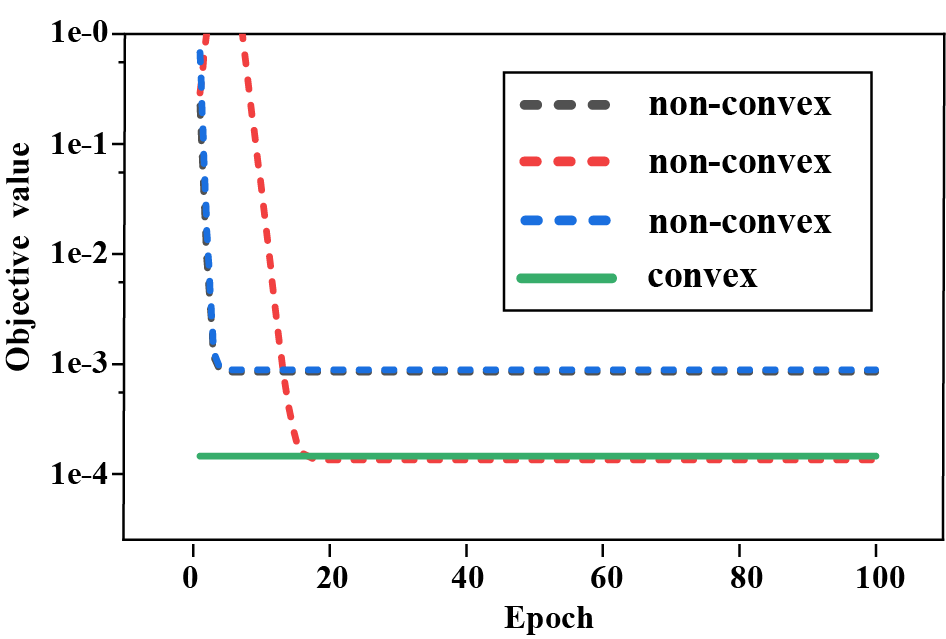
Figure 1: Toy example: In some bad cases, the non-convex neural network gets stuck in a local optimum or saddle point. The objective value of a two-layer non-convex and a convex neural network model for 1D vector fitting. The input of the network is $[-2,-1,0,1,2]^{T}$ and its ideal output (also called the label) is $[1,-1,-1,-1,1]^{T}$. Here, the bias term is included by concatenating a column of ones to the input. Under 3 random initialization trials of network parameters, the objective value of the non-convex neural network is different. Convex neural networks, which do not depend on the initialization, can be solved directly with a convex procedure to obtain the optimal value.

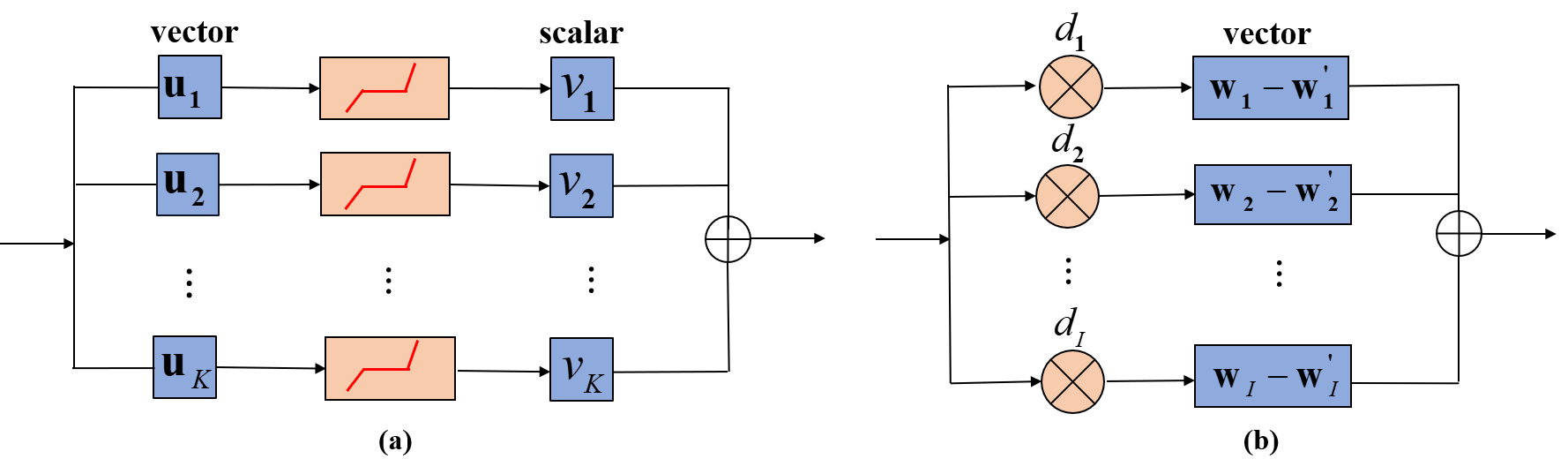
Figure 2: Neural network structures. (a) Primal ST-CNN, (b) dual ST-CNN.

Typical initialization strategies have been established[3, 15, 16] but the network may still encounter instability if the NN has multiple layers or branches[13]. For example, the original Transformer model [17] did not converge without initializing the learning rate in a warm-up way [18, 19, 20]. Roberta [21] and GPT-3 [22] had to tune the parameters of the optimizer ADAM[23] for stability under the large batch size. Recent studies have shown that architecture-specific initialization can promote convergence [19, 24, 25, 26, 27]. Even though, these initialization techniques hardly work to their advantage when conducting architecture searches, training networks with branching or heterogeneous components[13].

Convexifying neural networks is another way to make the solution not depend on initialization[28],[29]. At present, theoretical research on the convexification of NN focuses on finite-width networks which include fully connected networks[30, 31, 32, 33, 34, 35, 36, 37] and convolutional neural networks (CNN)[38, 39]. The former is powerful to learn multi-level features[40] but may require a large space and computational resources if the size of training data is large. The latter avoids this problem by reducing network complexity through local convolutions[41, 42, 43] and have been successfully applied in image processing[44, 45, 46, 47]. Up to now, CNN has been utilized as an example in convexifying networks under a common non-linear function, ReLU[38, 39].

To make the rest description clear, following previous theoretical work [38], we will adopt the denoising task handled by a basic two layers ReLU-CNN, for theoretical analysis of convexity.

Let $\widetilde{\textbf{X}}\in\mathbb{R}^{n\times h}$ denote a noise-free 2D image, $n$ and $h$ represent the width and height, respectively. $\widetilde{\textbf{X}}$ is contaminated by an additive noise E, whose entries are drawn from a probability distribution, such as $\mathscr{N}(0,\sigma^{2})$ in the case of i.i.d Gaussian noise. Then, the noisy observation $\widetilde{\textbf{Y}}$ is modeled as $\widetilde{\textbf{Y}}=\widetilde{\textbf{X}}+\textbf{E}$. Given a set of convolution filters, $\widetilde{\textbf{U}}_{k}\in\mathbb{R}^{m\times m}(k=1,...,K)$, noise-suppressed images are obtained under each filter and then linearly combined according to[38]

$$\sum_{k=1}^{K}\left(\widetilde{\textbf{Y}}\otimes\widetilde{\textbf{U}}_{k}\right)_{+}\otimes\widetilde{v}_{k},$$ (1)

where $\otimes$ represents the 2D convolution operation, $(\cdot)_{+}$ denotes an element-wise ReLU operation, and $\widetilde{v}_{k}\in\mathbb{R}$ is a 1×1 kernel used as the weight in the linear combination. Then, convolution kernels, i.e. $\widetilde{\textbf{U}}_{k}$ and $v_{k}$, are obtained by minimizing the prediction loss between the noise-free image and the network output as

$$\min_{\widetilde{\textbf{U}}_{k},\widetilde{v}_{k}}\left\|\sum_{k=1}^{K}\left(\widetilde{\textbf{Y}}\otimes\widetilde{\textbf{U}}_{k}\right)_{+}\otimes\widetilde{v}_{k}-\widetilde{\textbf{X}}\right\|_{F}^{2}.$$ (2)

To reduce the network complexity, Eq. (2) is further improved to an object value as[38]

$$\min_{\widetilde{\textbf{U}}_{k},\widetilde{v}_{k}}\left\|\sum_{k=1}^{K}\left(\widetilde{\textbf{Y}}\otimes\widetilde{\textbf{U}}_{k}\right)_{+}\otimes\widetilde{v}_{k}-\widetilde{\textbf{X}}\right\|_{F}^{2}$$ (3)

$$+\beta\sum_{k=1}^{K}(\left\|\widetilde{\textbf{U}}_{k}\right\|_{F}^{2}+|\widetilde{v}_{k}|^{2}),$$

by constraining the energy (or the power of norm) of all convolution kernels. The $\beta>0$ is a hyper-parameter to trade the prediction loss with the convolution kernel energy.

To convexify the primal network in Eq. (3), the convex duality theory was introduced to convert Eq. (3) into a dual form, enabling the reach of global minimum[38]. No gap between the primal and dual objective values has been demonstrated theoretically and experimentally[38]. This work inspired us to convexify other networks, for example, replacing ReLU with soft-thresholding.

Soft-thresholding (ST) is another non-linear function that has been widely adopted in CNN[48, 49, 50, 51, 7]. To the best of our knowledge, the convex form of primal Two-Layer Convolutional Neural Networks with Soft-Thresholding (primal ST-CNN) has not been set up. This work is to design its convex structure and provide the theoretical analysis (Fig. 2). First, we derive the weak duality of the primal ST-CNN using the Lagrange dual theory. Second, the nonlinear operation is converted into a linear operation (Fig. 3), which is used to divide hyperplanes and provide exact representations in the training process. Third, we theoretically prove that the strong duality holds between the two-layer primal ST-CNN (Fig. 2(a)) and its dual form (dual ST-CNN) (Fig. 2(b)). Finally, experiments are conducted to support theoretical findings.

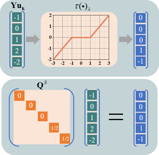
Figure 3: Toy example: Converting non-linear operation to linear operation. (a) Soft-thresholding in the primal ST-CNN, (b) diagonal matrix in the dual ST-CNN.

The rest of this paper is organized as follows: Section II introduces preliminaries. Section III presents the main theorem. Section IV shows experimental results and Section V makes the conclusion.

II Preliminaries

II-A Notations

Matrices and vectors are denoted by uppercase and lowercase bold letters, respectively. $\left\|\cdot\right\|_{2}$ and $\left\|\cdot\right\|_{F}$ represents Euclidean and Frobenius norms, respectively. We partition $P_{s}\subset\mathbb{R}^{m^{2}}$ into the following subsets

$$P_{s}=l_{1}\cup l_{2}\cup l_{3},$$ (4)

where

$$l_{1}=\{\textbf{u}_{k}|~{}\textbf{y}_{i}^{T}\textbf{u}_{k}\leq-\lambda\},~{}~{}~{}~{}~{}~{}~{}H_{1}=\{i|~{}\textbf{y}_{i}^{T}\textbf{u}_{k}\leq-\lambda\},$$ (5)

$$l_{2}=\{\textbf{u}_{k}|~{}-\lambda\leq\textbf{y}_{i}^{T}\textbf{u}_{k}\leq\lambda\},H_{2}=\{i|~{}-\lambda\leq\textbf{y}_{i}^{T}\textbf{u}_{k}\leq\lambda\},$$

$$l_{3}=\{\textbf{u}_{k}|~{}\textbf{y}_{i}^{T}\textbf{u}_{k}\geq\lambda\},~{}~{}~{}~{}~{}~{}~{}~{}~{}H_{3}=\{i|~{}\textbf{y}_{i}^{T}\textbf{u}_{k}\geq\lambda\},$$

$$\{\textbf{y}_{i}\in{\mathbb{R}^{m^{2}}\}}_{i=1}^{I},~{}I=nh,~{}~{}\textbf{u}_{k}\in{\mathbb{R}^{m^{2}}},~{}~{}\lambda\in\mathbb{R}.$$

We denote

$$S=S_{1}\cup S_{2}\cup S_{3},$$ (6)

where

$$S_{1}=\{i|~{}i\in H_{1}\}\cup\{i|~{}i\in H_{2}\},$$ (7)

$$S_{2}=\{i|~{}i\in H_{2}\},$$

$$S_{3}=\{i|~{}i\in H_{2}\}\cup\{i|~{}i\in H_{3}\}.$$

$$\textbf{Y}=[\textbf{y}_{1},\textbf{y}_{2},...,\textbf{y}_{I}]^{\top}\in{\mathbb{R}^{I\times m^{2}}},~{}~{}\textbf{Q}^{S}\in{\mathbb{R}^{I\times I}}~{}\text{is a}$$

diagonal matrix, its diagonal elements are as follows

$$\textbf{Q}_{ii}=\left\{\begin{matrix}&\\ \frac{\textbf{y}_{i}^{T}\textbf{u}_{k}+\lambda}{\textbf{y}_{i}^{T}\textbf{u}_{k}},\quad\text{if}\quad i\in S_{1},\\ &\\ \quad 0,\quad\quad\text{if}\quad i\in S_{2},\\ &\\ \frac{\textbf{y}_{i}^{T}\textbf{u}_{k}-\lambda}{\textbf{y}_{i}^{T}\textbf{u}_{k}},\quad\text{if}\quad i\in S_{3}.\end{matrix}\right.$$ (8)

$$\textbf{Q}^{S}=\textbf{Q}^{S_{1}}+\textbf{Q}^{S_{2}}+\textbf{Q}^{S_{3}},$$ (9)

We denote

$$\textbf{Q}^{S}~{}\text{in}~{}\text{Q}^{S}\textbf{Y}\textbf{u}_{k}\geq 0~{}\text{as}~{}\textbf{Q}^{S_{1}},$$

$$\textbf{Q}^{S}~{}\text{in}~{}\textbf{Q}^{S}\textbf{Y}\textbf{u}_{k}=0~{}\text{as}~{}\textbf{Q}^{S_{2}},$$

$$\textbf{Q}^{S}~{}\text{in}~{}\textbf{Q}^{S}\textbf{Y}\textbf{u}_{k}\leq 0~{}\text{as}~{}\textbf{Q}^{S_{2}}.$$

$$P_{S}=\{\textbf{u}_{k}|~{}P_{S_{1}}\cup P_{S_{2}}\cup P_{S_{3}}\},$$ (10)

where

$$P_{S_{1}}=\{\textbf{u}_{k}|~{}\textbf{Q}^{S_{1}}\textbf{Y}\textbf{u}_{k}\geq 0,\quad\forall i\in S_{1}\},$$ (11)

$$P_{S_{2}}=\{\textbf{u}_{k}|~{}\textbf{Q}^{S_{2}}\textbf{Y}\textbf{u}_{k}=0,\quad\forall i\in S_{2}\},$$

$$P_{S_{3}}=\{\textbf{u}_{k}|~{}\textbf{Q}^{S_{3}}\textbf{Y}\textbf{u}_{k}\leq 0,\quad\forall i\in S_{3}\}.$$

II-B Basic Lemmas and Definitions

Lemma 1 (Slater’s condition[52]): Consider the optimization problem

$$~{}~{}~{}~{}~{}~{}~{}~{}~{}~{}~{}~{}~{}\min_{\textbf{x}}f_{0}(\textbf{x})$$ (12)

$$~{}~{}~{}~{}~{}~{}~{}~{}~{}~{}~{}~{}~{}~{}\text{s.t.}~{}f_{j}(\textbf{x})<0,\quad j=1,...,J,\quad\textbf{Ax}=\textbf{b},$$

where $\textbf{A}\in\mathbb{R}^{m\times n}$, $\textbf{x}\in\mathbb{R}^{n}$, $\textbf{b}\in\mathbb{R}^{m}$, $f_{0},...,f_{J}$ are convex functions.

If there exists an $\textbf{x}^{*}\in\textbf{relint}D$ (where relint denotes the relative interior of the convex set $D:=\cap_{j=0}^{J}\text{dom}(f_{j})$), such that

$$f_{j}(\textbf{x}^{*})<0,\quad j=0,...,J,\quad\textbf{A}\textbf{x}^{*}=\textbf{b}.$$ (13)

Such a point is called strictly feasible since the inequality constraints hold with strict inequalities. The strong duality holds if Slater’s condition holds (and the problem is convex).

Lemma 2 (Sion’s Minimax theorem [53],[54]): Let $X$ and $Y$ be nonvoid convex and compact subsets of two linear topological spaces, and let $f:X\times Y\to\mathbb{R}$ be a function that is upper semicontinuous and quasi-concave in the first variable and lower semicontinuous and quasi-convex in the second variable. Then

$$\min_{y\in{Y}}\max_{x\in{X}}f(x,y)=\max_{x\in{X}}\min_{y\in{Y}}f(x,y).$$ (14)

Lemma 3 (Semi-infinite programming [55]): Semi-infinite programming problems of the form

$$\min_{\textbf{x}\in\mathbb{R}^{n}}f(\textbf{x})~{}\text{subject to}~{}g(\textbf{x},w)\leq 0,w\in\Omega,$$ (15)

where $\Omega$ is a (possibly infinite) index set, $\mathbb{\overline{R}}=\mathbb{R}\cup\{{+\infty}\}\cup\{{-\infty}\}$ denotes the extended real line, $f:\mathbb{R}^{n}\to\mathbb{\overline{R}}$ and $g:\mathbb{R}^{n}\times\Omega\to\mathbb{R}$. The above optimization problem is performed in the finite-dimensional space $\mathbb{R}$ and, if the index set $\Omega$ is infinite, is subject to an infinite number of constraints, therefore, it is referred to as a semi-infinite programming problem.

Lemma 4 (An extension of Zaslavsky’s hyperplane arrangement theory[56]): Consider a deep rectifier network with $L$ layers, $n_{l}$ rectified linear units at each layer $l$, and an input of dimension $n_{0}$. The maximal number of regions of this neural network is at most

$$\sum_{(j_{1},...,j_{L})}\prod_{l=1}^{L}\left(\begin{matrix}n_{l}\\ j_{l}\end{matrix}\right),$$ (16)

where $J=\{(j_{1},...,j_{L})\in\mathbb{Z}^{L}:0\leq j_{l}\leq\text{min}\{n_{0},n_{1}\!-\!j_{1},...,$
$n_{l-1}\!-\!j_{l-1},n_{l}\}~{}\forall~{}l=1,...,L\}.$ This bound is tight when $L=1$.

Definition 1 (Optimal duality gap[52]): The optimal value of the Lagrange dual problem is denoted as $d^{\ast}$, and the optimal value of the primal problem is denoted as $p^{\ast}$. The weak duality is defined as $d^{\ast}$ is the best lower bound of $p^{*}$ as follows

$$d^{\ast}\leq p^{\ast}.$$ (17)

The difference $p^{\ast}-d^{\ast}$ is called the optimal duality gap of the primal problem.

Definition 2 (Zero duality gap [52]): If the equality

$$d^{\ast}=p^{\ast}$$ (18)

holds, i.e. the optimal duality gap is zero, then we say that the strong duality holds. Strong duality means that a best bound, which can be obtained from the Lagrange dual function, is tight.

Definition 3 (Hyperplanes and halfspaces[52]):

A hyperplane is a set of the form $\{\textbf{x}|~{}\textbf{a}^{T}\textbf{x}=b\}$ where $\textbf{a}\in\mathbb{R}^{n},~{}\textbf{x}\in\mathbb{R}^{n\times 1},~{}\textbf{a}\neq 0$ and $b\in\mathbb{R}$.

A hyperplane divides $\mathbb{R}^{n}$ into halfspaces. A halfspace is a set of the form $\{\textbf{x}|~{}\textbf{a}^{T}\textbf{x}\leq b\}$ where $\textbf{a}\neq 0$, i.e. the solution set of one (nontrivial) linear inequality. This is illustrated in Fig. 4.

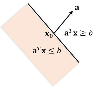
Figure 4: A hyperplane defined by $\textbf{a}^{\top}\textbf{x}=b$ in $\mathbb{R}^{2}$ determines two halfspaces. The halfspace determined by $\textbf{a}^{\top}\textbf{x}\geq b$ is the halfspace extending in the direction a. The halfspace determined by $\textbf{a}^{\top}\textbf{x}\leq b$ extends in the direction $-\textbf{a}$. The vector a is the outward of this halfspace.

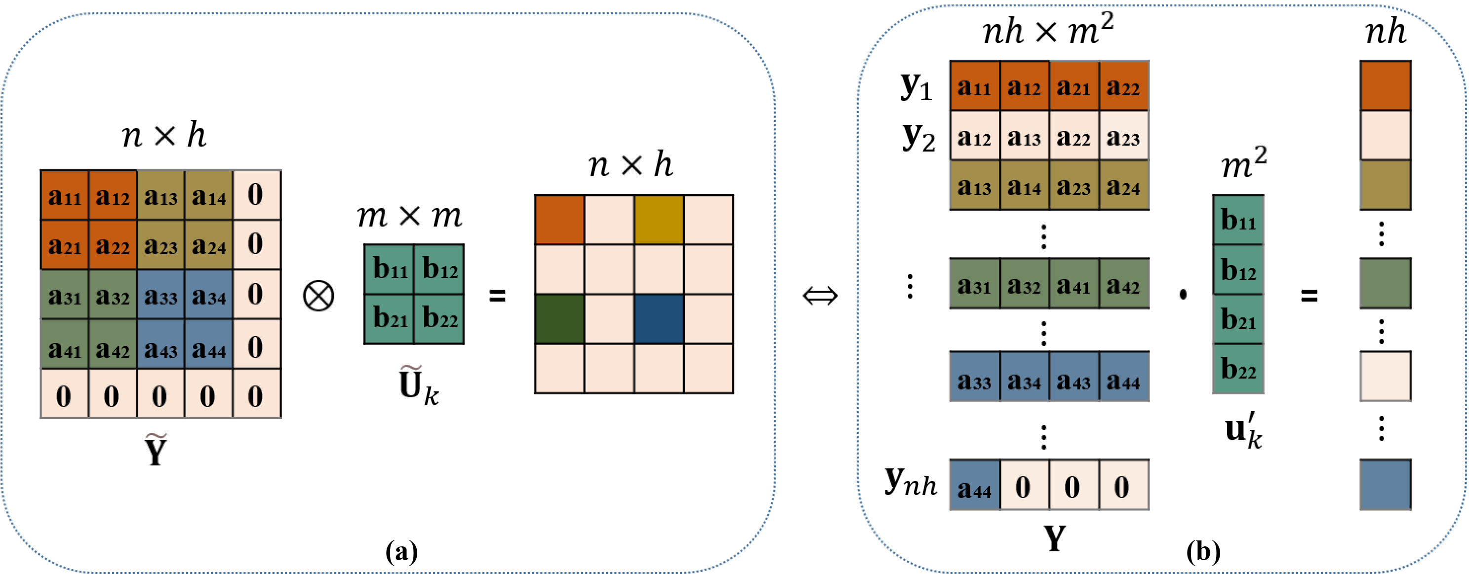
Figure 5: Replacing convolutional operations with matrix multiplication. (a) Convolution in Eq. (19), (b) matrix multiplication in Eq. (20).

III Model and Theory

III-A Proposed Model

A two-layer primal ST-CNN is expressed as follows

$$p^{\ast}= \min_{\widetilde{\textbf{U}}_{k},\widetilde{v}_{k}}\left\|\sum_{k=1}^{K}\tau\left(\widetilde{\textbf{Y}}\otimes\widetilde{\textbf{U}}_{k}\right)_{\lambda}\otimes\widetilde{v}_{k}-\widetilde{\textbf{X}}\right\|_{F}^{2}$$

$$+\beta\sum_{k=1}^{K}(\left\|\widetilde{\textbf{U}}_{k}\right\|_{F}^{2}+|\widetilde{v}_{k}|^{2}),$$ (19)

where the main difference between Eq. (19) and Eq. (3) is an element-wise soft-thresholding operator $\tau(a_{ij})_{\lambda}=(|a_{ij}|-\lambda)_{+}sign(a_{ij})$, $\otimes$ represents the 2D convolution operation, $\widetilde{\textbf{Y}}\in\mathbb{R}^{n\times h}$ is the input, $\widetilde{\textbf{U}}_{k}\in\mathbb{R}^{m\times m}$, $\widetilde{v}_{k}\in\mathbb{R}$, $\beta>0$.

Replacing convolutional operations with matrix multiplication (Fig. 5), Eq. (19) can be converted into the following form

$$p^{\ast}= \min_{\textbf{u}^{\prime}_{k},v^{\prime}_{k}}\left\|\sum_{k=1}^{K}\tau\left(\textbf{Y}\textbf{u}^{\prime}_{k}\right)_{\lambda}v^{\prime}_{k}-\textbf{x}\right\|_{2}^{2}$$

$$+\beta\sum_{k=1}^{K}(\left\|\textbf{u}^{\prime}_{k}\right\|_{2}^{2}+|v^{\prime}_{k}|^{2}),$$ (20)

where $\textbf{Y}=[\textbf{y}_{1},\textbf{y}_{2},...,\textbf{y}_{I}]^{\top}\in{\mathbb{R}^{I\times m^{2}}}$ is the input, $I=nh,$ $\{\textbf{y}_{i}\in{\mathbb{R}^{m^{2}}\}}_{i=1}^{I}$, $\textbf{x}\in\mathbb{R}^{I}$ is the label, $\textbf{u}^{\prime}_{k}\in{\mathbb{R}^{m^{2}}},v^{\prime}_{k}\in\mathbb{R}$.

Next, we introduce the main theory (Theorem 1) that converts a two-layer primal ST-CNN (Fig. 6(a)) into a convex dual ST-CNN (Fig. 6(b)).

Figure 6: Objective value of a two-layer primal ST-CNN and dual ST-CNN trained with ADAM on a one-dimensional dataset. Assuming $\textbf{x}=[-1,2,0,1,2]$ and $\textbf{y}=[2,1,2,1,2]$, which are the input and output, respectively. (a) Non-convex primal ST-CNN, (b) convex dual ST-CNN.

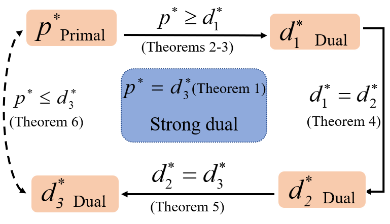
Figure 7: The main derivation process.

III-B Theoretical Analysis

Theorem 1 (Main theory): There exists $k^{*}\leq I$ such that if the number of convolution filters $k\geq(k^{*}+1)$, a two-layer ST-CNN (Eq. 20) has a strong duality satisfy form. This form is given through finite-dimensional convex programming as

$$d_{3}^{*}=\min_{\textbf{w}_{i}\in p_{w},\textbf{w}^{\prime}_{i}\in p_{w^{\prime}}} \left\|\sum_{i=1}^{I}\textbf{Q}^{S}\textbf{Y}(\textbf{w}^{\prime}_{i}-\textbf{w}_{i})-\textbf{x}\right\|_{2}^{2}$$ (21)

$$+2\beta\sum_{i=1}^{I}(\left\|\textbf{w}^{\prime}_{i}\right\|_{2}+\left\|\textbf{w}_{i}\right\|_{2}),$$

where $\textbf{Q}^{S}$ is a diagonal matrix, and its diagonal elements for $\textbf{Q}_{ii}$ take the following values

$$\textbf{Q}_{ii}=\left\{\begin{matrix}&\\ \frac{\textbf{y}_{i}^{T}\textbf{u}_{k}+\lambda}{\textbf{y}_{i}^{T}\textbf{u}_{k}},\quad\text{if}\quad i\in S_{1},\\ &\\ \quad 0,\quad\quad\text{if}\quad i\in S_{2},\\ &\\ \frac{\textbf{y}_{i}^{T}\textbf{u}_{k}-\lambda}{\textbf{y}_{i}^{T}\textbf{u}_{k}},\quad\text{if}\quad i\in S_{3}.\end{matrix}\right.$$ (22)

$\textbf{Y}=[\textbf{y}_{1},\textbf{y}_{2},...,\textbf{y}_{I}]^{\top}\in{\mathbb{R}^{I\times m^{2}}}$, $\textbf{w}_{i}$ and $\textbf{w}_{i}^{\prime}$ are both dual variables, and they correspond to $\textbf{u}^{\prime}_{k}$ and $v_{k}^{\prime}$ in Eq. (20) which are learnable parameters. $\textbf{x}\in\mathbb{R}^{I}$ is the label.

$$p_{w}=\left\{\textbf{w}_{i}|\textbf{Q}^{S_{1}}\textbf{Y}\textbf{w}_{i}\geq 0,\textbf{Q}^{S_{2}}\textbf{Y}\textbf{w}_{i}=0,\textbf{Q}^{S_{3}}\textbf{Y}\textbf{w}_{i}\leq 0\right\},$$ (23)

$$p_{w^{\prime}}=\left\{\textbf{w}^{\prime}_{i}|\textbf{Q}^{S_{1}}\textbf{Y}\textbf{w}^{\prime}_{i}\geq 0,\textbf{Q}^{S_{2}}\textbf{Y}\textbf{w}^{\prime}_{i}=0,\textbf{Q}^{S_{3}}\textbf{Y}\textbf{w}^{\prime}_{i}\leq 0\right\}.$$

$$\textbf{Q}^{S}=\textbf{Q}^{S_{1}}+\textbf{Q}^{S_{2}}+\textbf{Q}^{S_{3}}.$$ (24)

Remark: The constraints on w and $\textbf{w}^{\prime}$ in $p_{w}$ and $p_{w}^{\prime}$ arise from the segmentation property of the soft thresholding. We first randomly generate the vector $\bar{\textbf{w}}$ to do convolution with the input Y and generate the corresponding $\textbf{Q}^{S}$ based on the value of $\textbf{Y}\bar{\textbf{w}}$. Then we input Y and $\textbf{Q}^{S}$ into our dual ST-CNN, and Eq. (21) is used in our objective function (objective loss). Because it is an objective function with constraints $p_{w}$ and $p_{w}^{\prime}$, hence, we use hinge loss (adding constraints to the objective function) as the loss function in experiments. There exist $\textbf{w}_{i}$, $\textbf{w}^{\prime}_{i}$ such that $\bar{\textbf{w}}=\textbf{w}^{\prime}_{i}-\textbf{w}_{i}$.

Before proving the main theory (Theorem 1), we present the following main derivation framework (Fig. 7).

1) Theorem 2: Scaling $\left\|\textbf{u}^{\prime}_{k}\right\|_{2}^{2}+|v^{\prime}_{k}|^{2}$ in the primal ST-CNN (Eq. 20);

2) Theorem 3: Eliminating variables to obtain an equivalent convex optimization model under the principle of Lagrangian dual theory;

3) Theorem 4: Convert nonlinear operations to linear operations using a diagonal matrix;

4) Theorem 5: Exact representation of a two-layer ST-CNN;

5) Theorem 6: Prove zero dual gaps (strong duality).

Theorem 2: To scaling $\textbf{u}^{\prime}_{k},v^{\prime}_{k}$, let $\textbf{u}_{k}=\varepsilon\textbf{u}^{\prime}_{k}$, $v_{k}=\frac{1}{\varepsilon}{v^{\prime}}_{k}$,

$$p^{\ast}= \min_{\textbf{u}^{\prime}_{k},v^{\prime}_{k}}\left\|\sum_{k=1}^{K}\tau\left(\textbf{Y}\textbf{u}^{\prime}_{k}\right)_{\lambda}v^{\prime}_{k}-\textbf{x}\right\|_{2}^{2}$$

$$+\beta\sum_{k=1}^{K}(\left\|\textbf{u}^{\prime}_{k}\right\|_{2}^{2}+|v^{\prime}_{k}|^{2}),$$ (25)

the primal ST-CNN can be translated as

$$p^{\ast}= \min_{{\left\|\textbf{u}_{k}\right\|_{2}\leq 1}}\min_{v_{k}\in\mathbb{R}}\left\|\sum_{k=1}^{K}\tau\left(\textbf{Y}\textbf{u}_{k}\right)_{\lambda}v_{k}-\textbf{x}\right\|_{2}^{2}$$

$$+2\beta\sum_{k=1}^{K}(|v_{k}|),$$ (26)

where $\varepsilon$ is introduced so that the scaling has no effect on the network output, the proof of Theorem 2 is provided in Appendix A.

Then, according to Eq. (26), we can obtain an equivalent convex optimization model by using the Lagrangian dual theory.

Theorem 3:

$$p^{\ast}= \min_{{\left\|\textbf{u}_{k}\right\|_{2}\leq 1}}\min_{v_{k}\in\mathbb{R}}\left\|\sum_{k=1}^{K}\tau\left(\textbf{Y}\textbf{u}_{k}\right)_{\lambda}v_{k}-\textbf{x}\right\|_{2}^{2}$$

$$+2\beta\sum_{k=1}^{K}|{v}_{k}|.$$

is equivalent to

$$d_{1}^{\ast} =\max_{\left\|\textbf{u}_{k}\right\|_{2}\leq 1,\textbf{z}:|\textbf{z}^{T}\tau\left(\textbf{Y}\textbf{u}_{k}\right)_{\lambda}|\leq 2\beta}-\frac{1}{4}\left\|\textbf{z}-2\textbf{x}\right\|_{2}^{2}+\left\|\textbf{x}\right\|_{2}^{2}.$$ (27)

Proof: By reparameterizing the problem, let

$$\textbf{r}=\sum_{k=1}^{K}\tau\left(\textbf{Y}\textbf{u}_{k}\right)_{\lambda}v_{k}-\textbf{x},$$ (28)

where $\textbf{r}\in{\mathbb{R}^{I}}$, hence, we have

$$d_{1}^{\ast}=\min_{\left\|\textbf{u}_{k}\right\|_{2}\leq 1}\min_{{v}_{k},\textbf{r}}\left\|\textbf{r}\right\|_{2}^{2}+2\beta\sum_{k=1}^{K}|{v}_{k}|,$$

$$s.t.\quad\textbf{r}=\sum_{k=1}^{K}\tau\left(\textbf{Y}\textbf{u}_{k}\right)_{\lambda}v_{k}-\textbf{x}.$$ (29)

Introducing the Lagrangian variable z, and $\textbf{z}\in\mathbb{R}^{I}$, $\textbf{z}^{T}\in\mathbb{R}^{1\times I}$, and obtaining the Lagrangian dual form of the primal ST-CNN as follows

$$d_{1}^{\ast}= \min_{\left\|\textbf{u}_{k}\right\|_{2}\leq 1}\min_{v_{k},\textbf{r}}\max_{\textbf{z}}\left\|\textbf{r}\right\|_{2}^{2}+2\beta\sum_{k=1}^{K}|v_{k}|+\textbf{z}^{T}\textbf{r}$$

$$+\textbf{z}^{T}\textbf{x}-\textbf{z}^{T}\sum_{k=1}^{K}\tau\left(\textbf{Y}\textbf{u}_{k}\right)_{\lambda}v_{k}.$$ (30)

Using Sion’s minimax theorem[53],[54] to change the order of maximum and minimum

$$d_{1}^{\ast}= \min_{\left\|\textbf{u}_{k}\right\|_{2}\leq 1}\max_{\textbf{z}}\min_{v_{k},\textbf{r}}\left\|\textbf{r}\right\|_{2}^{2}+2\beta\sum_{k=1}^{K}|{v}_{k}|+\textbf{z}^{T}\textbf{r}$$

$$+\textbf{z}^{T}\textbf{x}-\textbf{z}^{T}\sum_{k=1}^{K}\tau\left(\textbf{Y}\textbf{u}_{k}\right)_{\lambda}v_{k}.$$ (31)

Minimizing the objective function Eq. (31) with r as a variable

$$\left\|\textbf{r}\right\|_{2}^{2}+\textbf{z}^{T}\textbf{r}=\left\|\textbf{r}+\frac{1}{2}\textbf{z}\right\|_{2}^{2}-\frac{1}{4}\left\|\textbf{z}\right\|_{2}^{2}.$$ (32)

When $\textbf{r}=-\frac{1}{2}\textbf{z}$, Eq. (31) takes the optimal value. Hence, Eq. (31) can be translated to

$$d_{1}^{\ast}= \min_{\left\|{\textbf{u}_{k}}\right\|_{2}\leq 1}\max_{\textbf{z}}\min_{v_{k}{}}-\frac{1}{4}\left\|\textbf{z}\right\|_{2}^{2}+2\beta\sum_{k=1}^{K}|{v}_{k}|+\textbf{z}^{T}\textbf{x}$$

$$-\textbf{z}^{T}\sum_{k=1}^{K}\tau\left(\textbf{Y}\textbf{u}_{k}\right)_{\lambda}v_{k}.$$ (33)

Let

$$f=\min_{v_{k}}2\beta\sum_{k=1}^{K}\left|v_{k}\right|-\textbf{z}^{T}\sum_{k=1}^{K}\tau\left(\textbf{Y}\textbf{u}_{k}\right)_{\lambda}v_{k},$$ (34)

eliminating the variable $v_{k}$ in the primal ST-CNN, hence

$$\max_{\textbf{z}:\left\|\textbf{u}_{k}\right\|_{2}\leq 1}|\textbf{z}^{T}\sum_{k=1}^{K}\tau\left(\textbf{Y}\textbf{u}_{k}\right)_{\lambda}|\leq 2\beta.$$ (35)

Eq. (33) is equivalent to the following optimization problem

$$d_{1}^{\ast} =\max_{\left\|\textbf{u}_{k}\right\|_{2}\leq 1,\textbf{z}:|\textbf{z}^{T}\sum_{k=1}^{K}\tau\left(\textbf{Y}\textbf{u}_{k}\right)_{\lambda}|\leq 2\beta}-\frac{1}{4}\left\|\textbf{z}-2\textbf{x}\right\|_{2}^{2}+\left\|\textbf{x}\right\|_{2}^{2}.$$ (36)

$\hfill\qed$

Next, to divide hyperplanes and provide an exact representation, we convert the nonlinear operation $\tau(\cdot)_{\lambda}$ into the linear operator using the diagonal matrix $\textbf{Q}^{S}$.

Theorem 4:

$$d_{1}^{\ast} =\max_{\left\|\textbf{u}_{k}\right\|_{2}\leq 1,\textbf{z}:|\textbf{z}^{T}\sum_{k=1}^{K}\tau\left(\textbf{Y}\textbf{u}_{k}\right)_{\lambda}|\leq 2\beta}-\frac{1}{4}\left\|\textbf{z}-2\textbf{x}\right\|_{2}^{2}+\left\|\textbf{x}\right\|_{2}^{2},$$

can be represented as a standard finite-dimensional program

$$d_{2}^{\ast}=\max_{\textbf{z}}-\frac{1}{4}\left\|\textbf{z}-2\textbf{x}\right\|_{2}^{2}+\left\|\textbf{x}\right\|_{2}^{2},$$ (37)

s.t.

$$P_{S}=\{\textbf{u}_{k}|~{}P_{S_{1}}\cup P_{S_{2}}\cup P_{S_{3}}\},$$ (38)

where

$$P_{S_{1}}=\{\textbf{u}_{k}|~{}\textbf{Q}^{S_{1}}\textbf{Y}\textbf{u}_{k}\geq 0,\quad\forall i\in S_{1}\},$$ (39)

$$P_{S_{2}}=\{\textbf{u}_{k}|~{}\textbf{Q}^{S_{2}}\textbf{Y}\textbf{u}_{k}=0,\quad\forall i\in S_{2}\},$$

$$P_{S_{3}}=\{\textbf{u}_{k}|~{}\textbf{Q}^{S_{3}}\textbf{Y}\textbf{u}_{k}\leq 0,\quad\forall i\in S_{3}\}.$$

Proof: First, we analyze the one-sided dual constraint in Eq. (35) as follows

$$\max_{\textbf{z}:\left\|\textbf{u}_{k}\right\|_{2}\leq 1}\textbf{z}^{T}\tau\left(\textbf{Y}\textbf{u}_{k}\right)_{\lambda}\leq 2\beta.$$ (40)

To divide hyperplanes, we divide $\mathbb{R}^{m^{2}}$ into three subsets to obtain Eq. (4) and Eq. (5). Let $i\in H_{1}\cup H_{2}\cup H_{3}$, $|H_{1}|+|H_{2}|+|H_{3}|=nh=I$, $\mathcal{H}_{X}$ be the set of all hyperplane arrangement patterns for the matrix Y, defined as the following set[57],[58]

$$\mathcal{H}_{X}=\{sign(\textbf{Y}\textbf{u}_{k}+\lambda)\cup sign(\textbf{Y}\textbf{u}_{k}-\lambda)|\textbf{u}_{k}\in{\mathbb{R}^{m^{2}}}\}.$$ (41)

Next, we take out the positions of the elements corresponding to different symbols and assign them according to

$$S_{1}=\{i|~{}i\in H_{1}\}\cup\{i|~{}i\in H_{2}\},$$ (42)

$$S_{2}=\{i|~{}i\in H_{2}\},$$

$$S_{3}=\{i|~{}i\in H_{2}\}\cup\{i|~{}i\in H_{3}\},$$

$$S=S_{1}\cup S_{2}\cup S_{3}.$$

To assign a corresponding value to the position of each $i$ in the above three sets such that the same transformation as the soft threshold function is achieved, the diagonal matrix $\textbf{Q}^{S}$ is constructed, and its diagonal elements for $\textbf{Q}_{ii}$ as Eq. (8).

Using the diagonal matrix $\textbf{Q}^{S}$, the constraints in Eq. (35) are equivalent to the following form

$$\max_{\begin{matrix}\left\|\textbf{u}_{k}\right\|_{2}\leq 1,P_{S}\end{matrix}}|\textbf{z}^{T}\textbf{Q}^{S}\left(\textbf{Y}\textbf{u}_{k}\right)|\leq 2\beta,$$ (43)

where $\textbf{Q}^{S}=\textbf{Q}^{S_{1}}+\textbf{Q}^{S_{2}}+\textbf{Q}^{S_{3}}$.

Hence, Eq. (36) can be finitely parameterized as

$$d^{\ast}_{2}=\max_{\textbf{z}}-\frac{1}{4}\left\|\textbf{z}-2\textbf{x}\right\|_{2}^{2}+\left\|\textbf{x}\right\|_{2}^{2},$$

s.t.

$$\max_{\begin{matrix}\left\|\textbf{u}_{k}\right\|_{2}\leq 1,P_{S}\end{matrix}}|\textbf{z}^{T}\textbf{Q}^{S}\textbf{Y}\textbf{u}_{k}|\leq 2\beta.$$ (44)

$\hfill\qed$

Now, we introduce an exact representation of a two-layer ST-CNN.

Theorem 5:

$$d^{\ast}_{2}=\max_{\textbf{z}}-\frac{1}{4}\left\|\textbf{z}-2\textbf{x}\right\|_{2}^{2}+\left\|\textbf{x}\right\|_{2}^{2},$$

s.t.

$$\max_{\begin{matrix}\left\|\textbf{u}_{k}\right\|_{2}\leq 1,P_{S}\end{matrix}}|\textbf{z}^{T}\textbf{Q}^{S}\textbf{Y}\textbf{u}_{k}|\leq 2\beta.$$

is equivalent to

$$d_{3}^{*}=\min_{\textbf{w}_{i}\in p_{w},\textbf{w}^{\prime}_{i}\in p_{w^{\prime}}} \left\|\sum_{i=1}^{I}\textbf{Q}^{S}\textbf{Y}(\textbf{w}^{\prime}_{i}-\textbf{w}_{i})-\textbf{x}\right\|_{2}^{2}$$ (45)

$$+2\beta\sum_{i=1}^{I}(\left\|\textbf{w}_{i}\right\|_{2}+\left\|\textbf{w}^{\prime}_{i}\right\|_{2}),$$

where,

$$p_{w}=\left\{\textbf{w}_{i}|\textbf{Q}^{S_{1}}\textbf{Y}\textbf{w}_{i}\geq 0,\textbf{Q}^{S_{2}}\textbf{Y}\textbf{w}_{i}=0,\textbf{Q}^{S_{3}}\textbf{Y}\textbf{w}_{i}\leq 0\right\},$$

$$p_{w^{\prime}}=\left\{\textbf{w}^{\prime}_{i}|\textbf{Q}^{S_{1}}\textbf{Y}\textbf{w}^{\prime}_{i}\geq 0,\textbf{Q}^{S_{2}}\textbf{Y}\textbf{w}^{\prime}_{i}=0,\textbf{Q}^{S_{3}}\textbf{Y}\textbf{w}^{\prime}_{i}\leq 0\right\}.$$

The proof of Theorem 5 is provided in Appendix B. According to this theorem, we can prove that the strong duality holds, i.e. the primal ST-CNN and the dual ST-CNN achieve global optimality. They are theoretically equivalent and will obtain Theorem 6.

Theorem 6: Suppose the optimal value of the primal ST-CNN is $p^{*}$ and the optimal value of the dual ST-CNN is $d^{*}_{3}$, the strong duality holds if $p^{*}=d^{*}_{3}$.

Proof: The optimal solution to the dual ST-CNN is the same as the optimal solution to the primal ST-CNN model constructed $\left\{\textbf{u}_{k}^{*},v_{k}^{*}\right\}_{k=1}^{K}$ as follows

$$(\textbf{u}_{k}^{*},v_{k}^{*})=(\frac{\textbf{w}_{i}^{*}}{\sqrt{\left\|\textbf{w}_{i}^{*}\right\|}},\sqrt{\left\|\textbf{w}_{i}^{*}\right\|}),\quad\text{if}\quad\textbf{w}_{i}^{*}\neq 0,$$

$$(\textbf{u}_{k}^{*},v_{k}^{*})=(\frac{{\textbf{w}^{\prime}}_{i}^{*}}{\sqrt{\left\|{\textbf{w}^{\prime}}_{i}^{*}\right\|}},\sqrt{\left\|{\textbf{w}^{\prime}}_{i}^{*}\right\|}),\quad\text{if}\quad{\textbf{w}^{\prime}}_{i}^{*}\neq 0,$$ (46)

where $\left\{\textbf{w}_{i}^{*},{\textbf{w}^{\prime}}_{i}^{*}\right\}_{i=1}^{I}$ are the optimal solution of Eq. (45).

$$p^{\ast}= \min_{\textbf{u}^{\prime}_{k}\in\mathbb{R}^{m},v^{\prime}_{k}\in\mathbb{R}}\left\|\sum_{k=1}^{K}\tau\left(\textbf{Y}\textbf{u}^{\prime}_{k}\right)_{\lambda}v^{\prime}_{k}-\textbf{x}\right\|_{2}^{2}$$ (47)

$$~{}~{}+\beta\sum_{k=1}^{K}(\left\|\textbf{u}^{\prime}_{k}\right\|_{2}^{2}+|v^{\prime}_{k}|^{2})$$

$$\leq\left\|\sum_{k=1}^{K}\tau\left(\textbf{Y}\textbf{u}^{*}_{k}\right)_{\lambda}v^{*}_{k}-\textbf{x}\right\|_{2}^{2}+\beta\sum_{k=1}^{I}(\left\|\textbf{u}^{*}_{k}\right\|_{2}^{2}+|v^{*}_{k}|^{2})~{}~{}~{}~{}~{}~{}~{}~{}~{}~{}~{}~{}~{}~{}~{}~{}~{}~{}~{}~{}~{}~{}~{}~{}$$

$$=\left\|\sum_{i=1}^{I}\textbf{Q}^{S}\textbf{Y}(\textbf{w}^{\prime}_{i}-\textbf{w}_{i})-\textbf{x}\right\|_{2}^{2}$$

$$~{}~{}+\beta\sum_{i=1,\textbf{w}_{i}^{*}\neq 0}^{I}\left(\left\|\frac{\textbf{w}_{i}^{*}}{\sqrt{\left\|\textbf{w}_{i}^{*}\right\|_{2}}}\right\|_{2}^{2}+\left\|\sqrt{\left\|\textbf{w}_{i}^{*}\right\|_{2}}\right\|_{2}^{2}\right)~{}~{}~{}~{}~{}~{}~{}~{}~{}~{}~{}~{}~{}~{}~{}~{}~{}~{}~{}~{}~{}~{}~{}~{}~{}~{}~{}~{}~{}~{}~{}$$

$$~{}~{}+\beta\sum_{i=1,\textbf{w}_{i}^{‘*}\neq 0}^{I}\left(\left\|\frac{{\textbf{w}^{\prime}}_{i}^{*}}{\sqrt{\left\|{\textbf{w}^{\prime}}_{i}^{*}\right\|_{2}}}\right\|_{2}^{2}+\left\|\sqrt{\left\|\textbf{w}_{i}^{’*}\right\|_{2}}\right\|_{2}^{2}\right)~{}~{}~{}~{}~{}~{}~{}~{}~{}~{}~{}~{}~{}~{}~{}~{}~{}~{}~{}~{}~{}~{}~{}~{}~{}~{}~{}~{}~{}~{}~{}$$

$$=\left\|\sum_{i=1}^{I}\textbf{Q}^{S}\textbf{Y}(\textbf{w}_{i}^{{}^{\prime}*}-\textbf{w}_{i}^{*})-\textbf{x}\right\|_{2}^{2}$$

$$~{}~{}+2\beta\sum_{i=1}^{I}\left(\left\|\textbf{w}_{i}^{*}\right\|_{2}+\left\|\textbf{w}_{i}^{{}^{\prime}*}\right\|_{2}\right)=d_{3}^{\ast}.~{}~{}~{}~{}~{}~{}~{}$$

Combining $p^{*}\leq d^{*}_{3}$, $p^{*}\geq d_{1}^{*}$ (Theorems 2-3) and $d_{1}^{*}=d_{2}^{*}=d_{3}^{*}$ (Theorems 4-5), $p^{*}=d^{*}_{3}$ is proved.

Basing on the Lemma 3[55], we know that $k+1$ of the total $I$ filters $(\textbf{w}_{i},\textbf{w}^{\prime}_{i})$ are non-zero at optimum, where $k\leq I$[38, 39].

Finally, by combining Theorems 2-6, the main theory can be proved. Thus, the hyperplane arrangements can be constructed in polynomial time (See proof in Appendix D).

The global optimization of neural networks is NP-Hard [59]. Despite the theoretical difficulty, highly accurate models are trained in practice using stochastic gradient methods [60]. Unfortunately, stochastic gradient methods cannot guarantee convergence to an optimum of the non-convex training loss [61] and existing methods rarely certify convergence to a stationary point of any type [62]. stochastic gradient methods are also sensitive to hyper-parameters, they converge slowly, to different stationary points [63] or even diverge depending on the choice of step size. Parameters like the random seed complicate replications and can produce model churn, where networks learned using the same procedure give different predictions for the same inputs [64][65].

Therefore, some optimizers were designed to find the optimal solution during the training process. For example, early on, the SGD optimizer [66], the SGD-based adaptive gradient optimizer (ASGD) [67] and the adoption of moment estimation (ADAM) [23] optimizer, may lead to different training results under the same non-convex optimization objective (See results in Section IV. A)[68].

IV Experimental Results

Experiments will show three observations: 1) The performance of the primal ST-CNN depends on the chosen optimizer. 2) The performance of the primal ST-CNN relies on initialization. 3) The zero dual gap holds between the primal and dual ST-CNN.

All experiments were implemented on a server equipped with dual Intel Xeon Silver 4210 CPUs, 128GB RAM, the Nvidia Tesla T4 GPU (16 GB memory), and PyTorch deep learning library[69]. The test dataset includes simulated data and the MNIST handwritten digits commonly used in deep learning research [38][70].

Experiments use the MNIST handwritten digits dataset with a size of 28×28. We randomly select 600 out of 60,000 as the training set, and 10,000 in the test set remain the same. Then, they are added i.i.d Gaussian noise from the distribution $\mathscr{N}(0,\sigma^{2})$ as the training and test dataset of the primal and the dual ST-CNN. For network training, 600 noisy images and their noise-free ones are used as the input and label. For the network test, 10000 noisy images and their noise-free ones are used as the input and label. The number of training and test datasets is consistent with that used in the ReLU-based dual theory experiments[38].

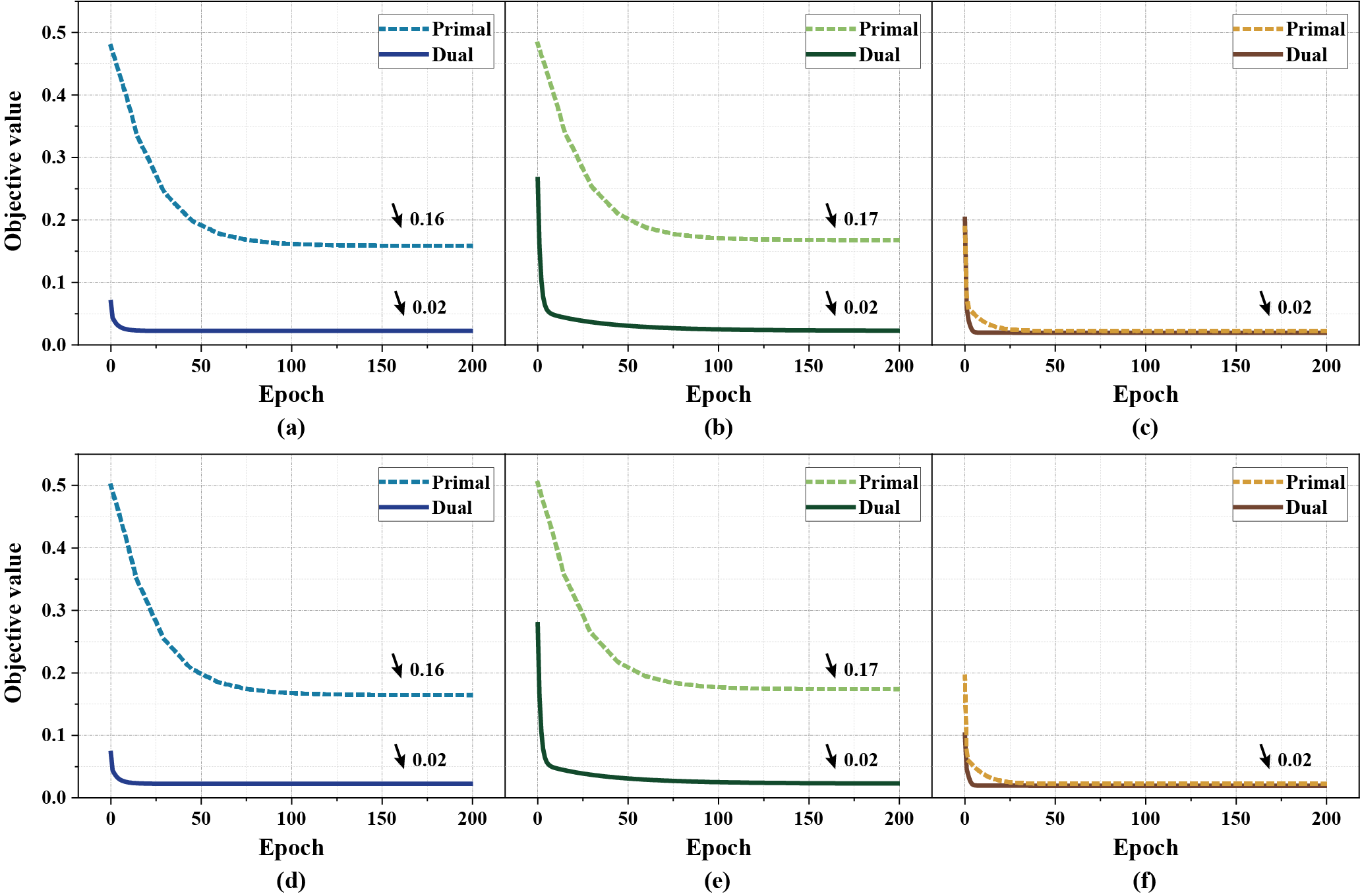
Figure 8: Training and testing with the different optimizers. From left to right: (a) Training results of the primal and primal ST-CNNs when SGD is used as an optimizer, (b) training results when the optimizer is ASGD, (c) training results when the optimizer is ADAM, (d) testing results when the optimizer is SGD, (e) testing results when the optimizer is ASGD, (f) testing results when the optimizer is ADAM.

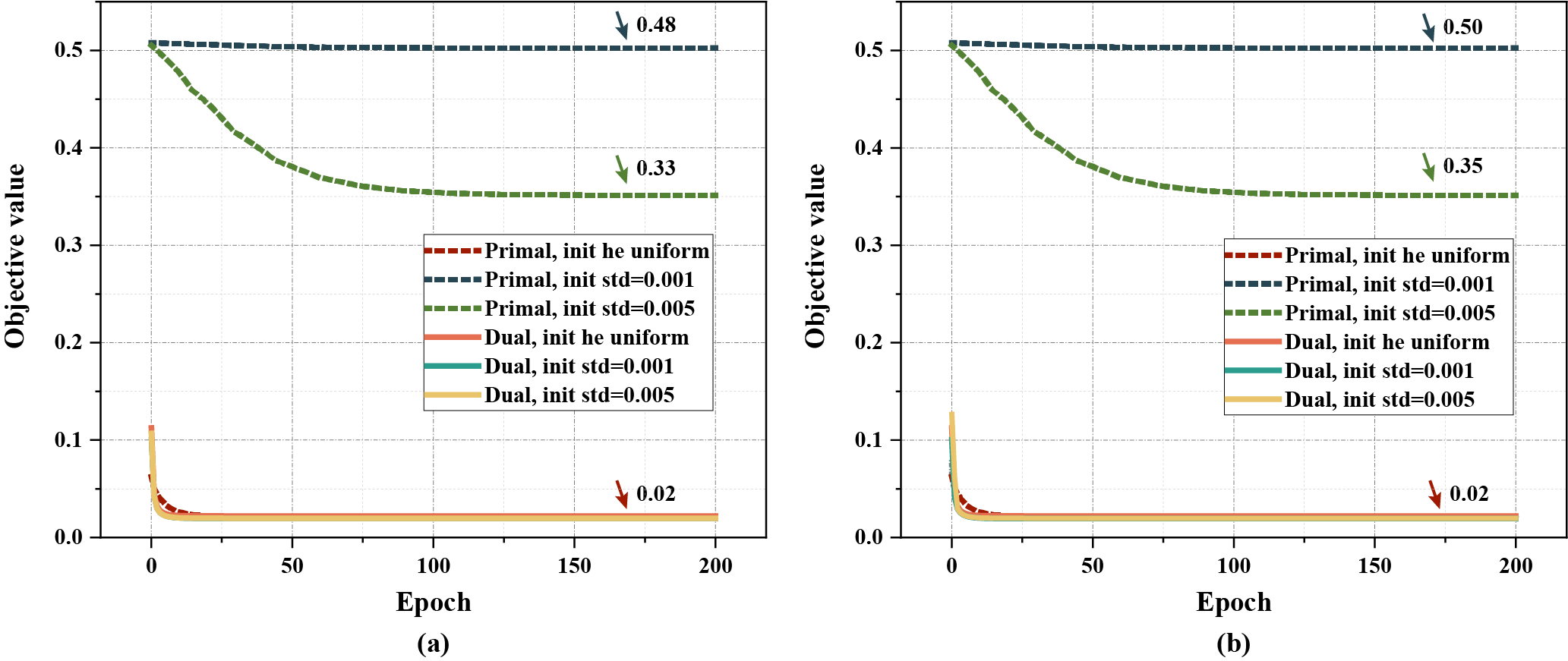
Figure 9: Example of training and testing with the different initialization. The primal ST-CNN and the dual ST-CNN are trained with Kaiming uniform initial[16], mean 0, standard deviation 0.001 and standard deviation 0.005 initialized with normal distribution, respectively. From left to right: (a) Training of the primal ST-CNN and dual ST-CNN. (b) Testing of the primal ST-CNN and dual ST-CNN.

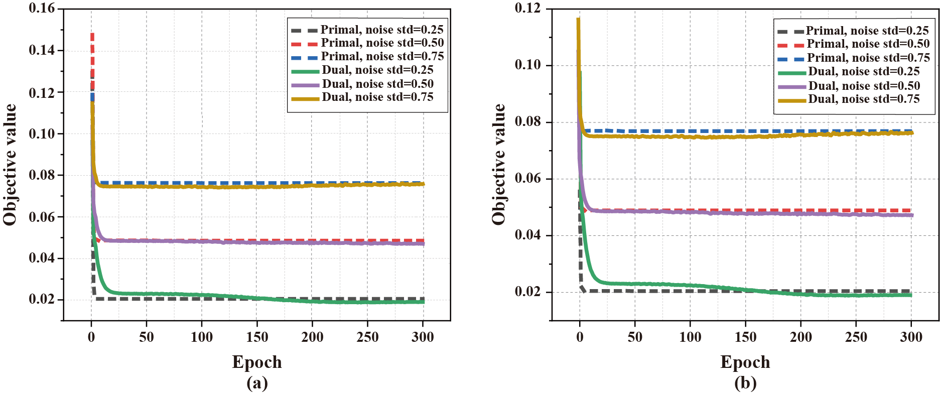
Figure 10: Verify that zero dual gap (the strong duality holds), i.e. the objective function values are very close when both the primal ST-CNN objective value and the dual network objective value achieves global optimality. (a) Training of the primal and dual ST-CNN in the case of Gaussian noise with mean 0 and standard deviation 0.25, 0.5, and 0.75 respectively. (b) Test of the primal and dual ST-CNNs in the case of Gaussian noise with a mean of 0 and standard deviations of 0.25, 0.5, and 0.75 respectively.

IV-A Primal ST-CNN Relies on Optimiser

Here, we choose noise $\sigma=0.25$, the primal ST-CNN and the dual ST-CNN are trained by using SGD, ASGD[67], and ADAM[23] as the optimizers respectively. The training and testing results are shown in Fig. 8. The optimal solution of the primal ST-CNN is dependent on the selection of optimizers.

IV-B Primal ST-CNN Relies on Initialization

We choose different ways of parameter initialization including Kaiming He uniform distribution initialized as well as a normal distribution with zero mean and standard deviation of 0.001 and 0.005, respectively. The experimental results are shown in Fig. 9. The objective value of the primal ST-CNN and the dual ST-CNN coincide when two types of networks are initialized with Kaiming He uniform distribution for training. However, when we initialize the network parameters using normal distributions with mean 0 and standard deviations of 0.001 and 0.005, the objective value of the dual ST-CNN will be better than the primal ST-CNN.

This observation implies that the primal ST-CNN is dependent on the selection of the initial values.

IV-C Verify Zero Dual Gap (Strong Duality)

Zero dual gap[52] means that, when both the primal and the dual ST-CNN reach the global optimum, the objective values of the two are equal. Therefore, according to the above two experimental results, in order to make the primal network achieve the global optimum, we choose ADAM[23] as the optimizer for the primal network, and the network parameters are initialized by Kaiming He uniform distribution. Under various noise levels $\sigma\in\{0.25,0.5,0.75\}$. Both approaches achieve close objective values under all noise levels (Fig. 10).

It should be noted here that the optimal values of the primal ST-CNN and the dual ST-CNN are not exactly equal as the theory proves, but very close. The error is caused by the fact that the experiment is based on a large amount of data training, which is within the negligible range. Hence, experimental results are consistent with our theory.

V Conclution

In this paper, to achieve the global optimum and remove the dependence of solutions on the initial network parameters, a convex dual ST-CNN is proposed to replace its primal ST-CNN (a convolution neural network with soft-thresholding). Under the principle of convex optimal dual theory, we theoretically prove that the strong duality holds between the dual and primal ST-CNN and further verify this observation in experiments of image denoising.

VI Appendix

VI-A Proof of Theorem 2

We combine basic inequality to rescale the parameters as $\left\|\textbf{u}^{\prime}_{k}\right\|_{2}^{2}+|v^{\prime}_{k}|^{2}$ in Eq. (20)[32],[37],[71, 72, 73].

The parameters can be rescaled $\textbf{u}^{\prime}_{k}=\varepsilon_{k}\textbf{u}_{k},$ and $v^{\prime}_{k}=\frac{v_{k}}{\varepsilon_{k}}$, for any $\varepsilon_{k}>0.$

$$\sum_{k=1}^{K}\tau\left(\textbf{Y}\textbf{u}^{\prime}_{k}\right)_{\lambda}v^{\prime}_{k}=\sum_{k=1}^{K}\tau\left(\varepsilon_{k}\textbf{Y}\textbf{u}_{k}\right)_{\lambda}\frac{v_{k}}{\varepsilon_{k}}=\sum_{k=1}^{K}\tau\left(\textbf{Y}\textbf{u}_{k}\right)_{\lambda}v_{k}.$$ (48)

This proves that the scaling has no effect on the network output. In addition to this, we have the following basic inequality

$$\min(\left\|\textbf{u}^{\prime}_{k}\right\|_{2}^{2}+|v^{\prime}_{k}|^{2})$$ (49)

$$=\min_{\varepsilon_{k}}(\left\|\varepsilon_{k}|\textbf{u}_{k}\right\|_{2}^{2}+\left|\frac{v_{k}}{\varepsilon_{k}}\right|^{2})$$

$$=2\min\left\|\textbf{u}_{k}\right\|_{2}\left|v_{k}\right|,$$

here $\varepsilon_{k}=(\frac{v_{k}}{\left\|\textbf{u}_{k}\right\|_{2}})^{\frac{1}{2}}.$

Since the scaling operation has no effect on the right-hand side of the inequality. we can set $\left\|\textbf{u}_{k}\right\|_{2}=1$, $\forall k$. Therefore, $\left\|\textbf{u}_{k}\right\|_{2}\left|v_{k}\right|$ becomes $\left|v_{k}\right|$.

Now, let us consider a modified version of the problem, where the unit norm inequality constraint has no effect on the optimal solution. Let us assume that for a certain index $k$, $\left\|\textbf{u}_{k}\right\|_{2}\leq 1$ exit $v_{k}\neq 0$ as an optimal solution. This shows that the unit norm inequality constraint is not activated for $v_{k}$ and hence removing the constraint for $\textbf{u}_{k}$ will not change the optimal solution.

However, removing the constraint $\left\|\textbf{u}_{k}\right\|_{2}\longrightarrow\infty$ reduces the objective value since it yields $v_{k}=0$.

Here, we have a contradiction that proves that all the constraints that correspond to a nonzero $v_{k}$ must be active for an optimal solution.

This also shows that replacing $\left\|\textbf{u}_{k}\right\|_{2}=1$ with $\left\|\textbf{u}_{k}\right\|_{2}\leq 1$ is the solution to the problem.

Hence,

$$p^{\ast}= \min_{\textbf{u}_{k}\in\mathbb{R}^{m},v_{k}\in\mathbb{R}}\left\|\sum_{k=1}^{K}\tau\left(\textbf{Y}\textbf{u}_{k}\right)_{\lambda}v_{k}-\textbf{x}\right\|_{2}^{2}$$

$$+2\beta\sum_{k=1}^{K}(\left\|\textbf{u}_{k}\right\|_{2}|v_{k}|).$$ (50)

Relaxing the constraints without changing the optimal solution of the objective function such that $\left\|\textbf{u}_{k}\right\|_{2}\leq 1$, so

$$p^{\ast}= \min_{{\left\|\textbf{u}_{k}\right\|_{2}\leq 1}}\min_{v_{k}\in\mathbb{R}}\left\|\sum_{k=1}^{K}\tau\left(\textbf{Y}\textbf{u}_{k}\right)_{\lambda}v_{k}-\textbf{x}\right\|_{2}^{2}$$ (51)

$$+2\beta\sum_{k=1}^{K}|{v}_{k}|.$$

$\hfill\qed$

VI-B Proof of Theorem 5

Here,

$$\max_{\begin{matrix}\left\|\textbf{u}_{k}\right\|_{2}\leq 1,P_{S}\end{matrix}}|\textbf{z}^{T}\textbf{Q}^{S}\left(\textbf{Y}\textbf{u}_{k}\right)|\leq 2\beta,$$ (52)

can be split into two constraints

$$\max_{\begin{matrix}\left\|\textbf{u}_{k}\right\|_{2}\leq 1,P_{S}\end{matrix}}\textbf{z}^{T}\textbf{Q}^{S}\left(\textbf{Y}\textbf{u}_{k}\right)\leq 2\beta,$$ (53)

and

$$\max_{\begin{matrix}\left\|\textbf{u}_{k}\right\|_{2}\leq 1,P_{S}\end{matrix}}-\textbf{z}^{T}\textbf{Q}^{S}\left(\textbf{Y}\textbf{u}_{k}\right)\leq 2\beta.$$ (54)

We first discuss the former

$$\max_{\begin{matrix}\left\|\textbf{u}_{k}\right\|_{2}\leq 1,P_{S}\end{matrix}}\textbf{z}^{T}\textbf{Q}^{S}\left(\textbf{Y}\textbf{u}_{k}\right)\Longrightarrow\min_{\begin{matrix}\left\|\textbf{u}_{k}\right\|_{2}\leq 1,P_{S}\end{matrix}}-\textbf{z}^{T}\textbf{Q}^{S}\left(\textbf{Y}\textbf{u}_{k}\right).$$ (55)

Introducing $\textbf{b},\textbf{c},\textbf{e}\in R^{I}$, the Lagrangian form of the above function as follows

$$L(\textbf{u}_{k})= -\textbf{z}^{\top}\textbf{Q}^{S}\textbf{Y}\textbf{u}_{k}-\textbf{b}\textbf{Q}^{S_{1}}\textbf{Y}\textbf{u}_{k}+\textbf{c}\textbf{Q}^{S_{2}}\textbf{Y}\textbf{u}_{k}$$

$$+\textbf{e}\textbf{Q}^{S_{3}}\textbf{Y}\textbf{u}_{k},$$ (56)

where

$$-(\textbf{z}^{\top}\textbf{Q}^{S}\textbf{Y}\textbf{u}_{k}-\textbf{b}\textbf{Q}^{S_{1}}\textbf{Y}\textbf{u}_{k}+\textbf{c}\textbf{Q}^{S_{2}}\textbf{Y}\textbf{u}_{k}+\textbf{e}\textbf{Q}^{S_{3}}\textbf{Y}\textbf{u}_{k})$$

$$= -(\textbf{z}^{\top}\textbf{Q}^{S}\textbf{Y}\textbf{u}_{k}+\textbf{b}\textbf{Q}^{S_{1}}\textbf{Y}\textbf{u}_{k}-\textbf{c}\textbf{Q}^{S_{2}}\textbf{Y}\textbf{u}_{k}-\textbf{e}\textbf{Q}^{S_{3}}\textbf{Y}\textbf{u}_{k})$$

$$\geq -\left\|\textbf{Y}^{\top}\textbf{Q}^{S}\textbf{z}+\textbf{Y}^{\top}\textbf{Q}^{S_{1}}\textbf{b}-\textbf{Y}^{\top}\textbf{Q}^{S_{2}}\textbf{c}-\textbf{Y}^{\top}\textbf{Q}^{S_{3}}\textbf{e}\right\|_{2}\left\|\textbf{u}_{k}\right\|_{2}.$$

Let $\left\|\textbf{u}_{k}\right\|_{2}=1,$

$$infL(\textbf{u}_{k})$$

$$=-\left\|\textbf{Y}^{\top}\textbf{Q}^{S}\textbf{z}+\textbf{Y}^{\top}\textbf{Q}^{S_{1}}\textbf{b}-\textbf{Y}^{\top}\textbf{Q}^{S_{2}}\textbf{c}-\textbf{Y}^{\top}\textbf{Q}^{S_{3}}\textbf{e}\right\|_{2}.$$ (57)

Then, the dual problem is as follows

$$\min_{\begin{matrix}\textbf{b},\textbf{c},\textbf{e}\in\mathbb{R}^{I}\\ \textbf{b},\textbf{e}\geq 0\end{matrix}}\left\|\textbf{Y}^{\top}\textbf{Q}^{S}\textbf{z}+\textbf{Y}^{\top}\textbf{Q}^{S_{1}}\textbf{b}-\textbf{Y}^{\top}\textbf{Q}^{S_{2}}\textbf{c}-\textbf{Y}^{\top}\textbf{Q}^{S_{3}}\textbf{e}\right\|_{2}.$$ (58)

Hence, the constraints

$$\max_{\textbf{z}:\left\|\textbf{u}_{k}\right\|_{2}\leq 1}\textbf{z}^{T}\tau\left(\textbf{Y}\textbf{u}_{k}\right)_{\lambda}\leq 2\beta,$$

can be equal as follows

$$\min_{\begin{matrix}\textbf{b},\textbf{c},\textbf{e}\in{\mathbb{R}^{I}}\\ \textbf{b},\textbf{e}\geq 0\end{matrix}}$$

$$\left\|\textbf{Y}^{\top}\textbf{Q}^{S}\textbf{z}+\textbf{Y}^{\top}\textbf{Q}^{S_{1}}\textbf{b}-\textbf{Y}^{\top}\textbf{Q}^{S_{2}}\textbf{c}-\textbf{Y}^{\top}\textbf{Q}^{S_{3}}\textbf{e}\right\|_{2}$$

$$\leq 2\beta.$$ (59)

According to the above equation, we can deduce that

$$\forall i\in{[1,I]},~{}\exists\quad\textbf{b}_{i},\textbf{c}_{i},\textbf{e}_{i}\in R^{I},~{}~{}s.t.~{}~{}\textbf{b}_{i},\textbf{e}_{i}\geq 0$$

$$\left\|\textbf{Y}^{\top}\textbf{Q}^{S}\textbf{z}+\textbf{Y}^{\top}\textbf{Q}^{S_{1}}\textbf{b}_{i}-\textbf{Y}^{\top}\textbf{Q}^{S_{2}}\textbf{c}_{i}-\textbf{Y}^{\top}\textbf{Q}^{S_{3}}\textbf{e}_{i}\right\|_{2}$$

$$\leq 2\beta.$$ (60)

Considering the constraints on both sides, introducing variables $\textbf{b}^{\prime}_{i},~{}\textbf{c}^{\prime}_{i},~{}\textbf{e}^{\prime}_{i}.$

Then, there are $2I$ constraints as follows:

$$\max_{\begin{matrix}\textbf{z}\\ \textbf{b}_{i},\textbf{c}_{i},\textbf{e}_{i}\in\mathbb{R}^{I}\\ \textbf{b}_{i},\textbf{e}_{i}\geq 0\\ \textbf{b}^{\prime}_{i},\textbf{c}^{\prime}_{i},\textbf{e}^{\prime}_{i}\in\mathbb{R}^{I}\\ \textbf{b}^{\prime}_{i},\textbf{e}^{\prime}_{i}\geq 0\end{matrix}}-\frac{1}{4}\left\|\textbf{z}-2\textbf{x}\right\|_{2}^{2}+\left\|\textbf{x}\right\|_{2}^{2},$$ (61)

s.t.

$$\left\|\textbf{Y}^{\top}\textbf{Q}^{S}\textbf{z}+\textbf{Y}^{\top}\textbf{Q}^{S_{1}}\textbf{b}_{1}-\textbf{Y}^{\top}\textbf{Q}^{S_{2}}\textbf{c}_{1}-\textbf{Y}^{\top}\textbf{Q}^{S_{3}}\textbf{e}_{1}\right\|_{2}$$

$$\leq 2\beta$$

$$~{}~{}~{}~{}~{}~{}~{}~{}~{}~{}~{}~{}~{}~{}~{}~{}~{}~{}~{}~{}~{}~{}~{}~{}~{}~{}~{}~{}~{}~{}~{}~{}~{}~{}~{}~{}~{}~{}~{}~{}\vdots$$

$$\left\|\textbf{Y}^{\top}\textbf{Q}^{S}\textbf{z}+\textbf{Y}^{\top}\textbf{Q}^{S_{1}}\textbf{b}_{I}-\textbf{Y}^{\top}\textbf{Q}^{S_{2}}\textbf{c}_{I}-\textbf{Y}^{\top}\textbf{Q}^{S_{3}}\textbf{e}_{I}\right\|_{2}$$

$$\leq 2\beta$$

$$\left\|-\textbf{Y}^{\top}\textbf{Q}^{S}\textbf{z}+\textbf{Y}^{\top}\textbf{Q}^{S_{1}}\textbf{b}^{\prime}_{1}-\textbf{Y}^{\top}\textbf{Q}^{S_{2}}\textbf{c}^{\prime}_{1}-\textbf{Y}^{\top}\textbf{Q}^{S_{3}}\textbf{e}^{\prime}_{1}\right\|_{2}$$

$$\leq 2\beta$$

$$~{}~{}~{}~{}~{}~{}~{}~{}~{}~{}~{}~{}~{}~{}~{}~{}~{}~{}~{}~{}~{}~{}~{}~{}~{}~{}~{}~{}~{}~{}~{}~{}~{}~{}~{}~{}~{}~{}~{}~{}\vdots$$

$$\left\|-\textbf{Y}^{\top}\textbf{Q}^{S}\textbf{z}+\textbf{Y}^{\top}\textbf{Q}^{S_{1}}\textbf{b}^{\prime}_{I}-\textbf{Y}^{\top}\textbf{Q}^{S_{2}}\textbf{c}^{\prime}_{I}-\textbf{Y}^{\top}\textbf{Q}^{S_{3}}\textbf{e}^{\prime}_{I}\right\|_{2}$$

$$\leq 2\beta.$$

Noting that, as long as $\beta>0$, let $\textbf{b}_{i}=\textbf{c}_{i}=\textbf{e}_{i}=\textbf{b}^{\prime}_{i}=\textbf{c}^{\prime}_{i}=\textbf{e}^{\prime}_{i}=\textbf{z}=\textbf{0}$, the above constraint holds, and the strong duality holds from the Slater’s condition.

The dual problem can be rewritten as

$$\min_{\begin{matrix}\lambda_{i},\lambda_{i}^{{}^{\prime}}\in\mathbb{R}\\ \lambda_{i},\lambda_{i}^{{}^{\prime}}\geq 0\end{matrix}}\max_{\begin{matrix}\textbf{z}\\ \textbf{b}_{i},\textbf{c}_{i},\textbf{e}_{i}\in\mathbb{R}^{I}\\ \textbf{b}_{i},\textbf{e}_{i}\geq 0\\ \textbf{b}^{\prime}_{i},\textbf{c}^{\prime}_{i},\textbf{e}^{\prime}_{i}\in\mathbb{R}^{I}\\ \textbf{b}^{\prime}_{i},\textbf{e}^{\prime}_{i}\geq 0\end{matrix}}$$ (62)

$$-\frac{1}{4}\left\|\textbf{z}-2\textbf{x}\right\|_{2}^{2}+\left\|\textbf{x}\right\|_{2}^{2}$$

$$+\sum_{i=1}^{I}2\lambda_{i}\beta+\sum_{i=1}^{I}2\lambda_{i}^{\prime}\beta$$

$$-\sum_{i=1}^{I}\lambda_{i}\left\|\textbf{Y}^{\top}(\textbf{Q}^{S}\textbf{z}+\textbf{Q}^{S_{1}}\textbf{b}_{i}-\textbf{Q}^{S_{2}}\textbf{c}_{i}-\textbf{Q}^{S_{3}}\textbf{e}_{i})\right\|_{2}$$

$$-\sum_{i=1}^{I}\lambda_{i}^{\prime}\left\|\textbf{Y}^{\top}(-\textbf{Q}^{S}\textbf{z}+\textbf{Q}^{S_{1}}\textbf{b}^{\prime}_{i}-\textbf{Q}^{S_{2}}\textbf{c}^{\prime}_{i}-\textbf{Q}^{S_{3}}\textbf{e}^{\prime}_{i})\right\|_{2}.$$

Introducing variable $\textbf{t}_{1},...,\textbf{t}_{I},\textbf{t}^{\prime}_{1},...,\textbf{t}^{\prime}_{I}\in\mathbb{R}^{m^{2}}$, the above formula can be changed to

$$\min_{\begin{matrix}\lambda_{i},\lambda_{i}^{{}^{\prime}}\in\mathbb{R}\\ \lambda_{i},\lambda_{i}^{{}^{\prime}}\geq 0\end{matrix}}\max_{\begin{matrix}\textbf{z}\\ \textbf{b}_{i},\textbf{c}_{i},\textbf{e}_{i}\in\mathbb{R}^{I}\\ \textbf{b}_{i},\textbf{e}_{i}\geq 0\\ \textbf{b}_{i}^{{}^{\prime}},\textbf{c}_{i}^{{}^{\prime}},\textbf{e}_{i}^{{}^{\prime}}\in\mathbb{R}^{I}\\ \textbf{b}_{i}^{{}^{\prime}},\textbf{e}_{i}^{{}^{\prime}}\geq 0\end{matrix}}\min_{\begin{matrix}\textbf{t}_{i}\in\mathbb{R}^{m^{2}},\left\|\textbf{t}_{i}\right\|_{2}\leq 1\\ \textbf{t}_{i}{’}\in\mathbb{R}^{m^{2}},\left\|\textbf{t}_{i}^{\prime}\right\|_{2}\leq 1\\ \forall i\in[1,I]\end{matrix}}$$ (63)

$$-\frac{1}{4}\left\|\textbf{z}-2\textbf{x}\right\|_{2}^{2}+\left\|\textbf{x}\right\|_{2}^{2}$$

$$+\sum_{i=1}^{I}2\beta(\lambda_{i}+\lambda_{i}^{{}^{\prime}})$$

$$+\sum_{i=1}^{I}\lambda_{i}\textbf{t}_{i}^{\top}\textbf{Y}^{\top}(-\textbf{Q}^{S}\textbf{z}-\textbf{Q}^{S_{1}}\textbf{b}_{i}+\textbf{Q}^{S_{2}}\textbf{c}_{i}+\textbf{Q}^{S_{3}}\textbf{e}_{i})$$

$$+\sum_{i=1}^{I}\lambda^{\prime}_{i}\textbf{t}_{i}^{{}^{\prime}\top}\textbf{Y}^{\top}(\textbf{Q}^{S}\textbf{z}-\textbf{Q}^{S_{1}}\textbf{b}^{\prime}_{i}+\textbf{Q}^{S_{2}}\textbf{c}^{\prime}_{i}+\textbf{Q}^{S_{3}}\textbf{e}^{\prime}_{i}).$$

Next, we take z, $\textbf{b}_{i},\textbf{b}^{\prime}_{i},\textbf{c}_{i},\textbf{c}^{\prime}_{i},\textbf{e}_{i},\textbf{e}^{\prime}_{i}$ as variables to analyze the maximum value of the objective function.

Where, we take z as the variable to analyze the following objective functions

$$-\frac{1}{4}\left\|\textbf{z}-2\textbf{x}\right\|_{2}^{2}-\sum_{i=1}^{I}\lambda_{i}\textbf{t}_{i}^{\top}\textbf{Y}^{\top}\textbf{Q}^{S}\textbf{z}+\sum_{i=1}^{I}\lambda_{i}^{{}^{\prime}}\textbf{t}_{i}^{{}^{\prime}\top}\textbf{Y}^{\top}\textbf{Q}^{S}\textbf{z}$$

$$= -\frac{1}{4}(\left\|\textbf{z}\right\|_{2}^{2}-4\textbf{z}^{\top}\textbf{x}+4\left\|\textbf{x}\right\|_{2}^{2})-\sum_{i=1}^{I}\lambda_{i}\textbf{t}_{i}^{\top}\textbf{Y}^{\top}\textbf{Q}^{S}\textbf{z}$$

$$+\sum_{i=1}^{I}\lambda_{i}^{{}^{\prime}}\textbf{t}_{i}^{{}^{\prime}\top}\textbf{Y}^{\top}\textbf{Q}^{S}\textbf{z}$$

$$= -\frac{1}{4}\left(\left\|\textbf{z}\right\|_{2}^{2}-4\textbf{z}^{\top}\textbf{x}+4\left\|\textbf{x}\right\|_{2}^{2}+4\sum_{i=1}^{I}\lambda_{i}\textbf{t}_{i}^{\top}\textbf{Y}^{\top}\textbf{Q}^{S}\textbf{z}\right)$$

$$+\sum_{i=1}^{I}\lambda^{\prime}_{i}\textbf{t}_{i}^{{}^{\prime}\top}\textbf{Y}^{\top}\textbf{Q}^{S}\textbf{z}$$

$$= -\frac{1}{4}\left\|\sum_{i=1}^{I}\textbf{z}-(2\textbf{x}-2\lambda_{i}\textbf{Q}^{S}\textbf{Y}\textbf{t}_{i}+2\lambda^{\prime}_{i}\textbf{Q}^{S}\textbf{Y}\textbf{t}_{i}^{{}^{\prime}})\right\|_{2}^{2}$$

$$-\left\|\textbf{x}\right\|_{2}^{2}$$

$$+\left\|\sum_{i=1}^{I}\textbf{x}-\lambda_{i}\textbf{Q}^{S}\textbf{Y}\textbf{t}_{i}+\lambda^{\prime}_{i}\textbf{Q}^{S}\textbf{Y}\textbf{t}^{\prime}_{i}\right\|.$$ (64)

Let $\textbf{z}=2\textbf{x}-2\lambda_{i}\textbf{Q}^{S}\textbf{Y}\textbf{t}_{i}+2\lambda^{\prime}_{i}\textbf{Q}^{S}\textbf{Y}\textbf{t}^{\prime}_{i}$, the objective function can take the maximum value

$$\min_{\begin{matrix}\lambda_{i},\lambda_{i}^{{}^{\prime}}\in\mathbb{R}\\ \lambda_{i}^{{}^{\prime}}\geq 0\end{matrix}}\min_{\begin{matrix}\textbf{t}_{i}\in\mathbb{R}^{m^{2}},\left\|\textbf{t}_{i}\right\|_{2}\leq 1\\ \textbf{t}^{\prime}_{i}\in\mathbb{R}^{m^{2}},\left\|\textbf{t}^{\prime}_{i}\right\|_{2}\leq 1\\ \forall i\in[1,I]\end{matrix}}\max_{\begin{matrix}\textbf{b}_{i},\textbf{b}^{\prime}_{i},\textbf{c}_{i},\textbf{c}^{\prime}_{i},\textbf{e}_{i},\textbf{e}^{\prime}_{i}\geq 0\\ \textbf{b}_{i},\textbf{b}^{\prime}_{i},\textbf{c}_{i},\textbf{c}^{\prime}_{i},\textbf{e}_{i},\textbf{e}^{\prime}_{i}\in\mathbb{R}^{I}\end{matrix}}$$

$$\left\|\sum_{i=1}^{I}(\textbf{x}-\lambda_{i}\textbf{Q}^{S}\textbf{Y}\textbf{t}_{i}+\lambda^{\prime}_{i}\textbf{Q}^{S}\textbf{Y}\textbf{t}^{\prime}_{i})\right\|_{2}^{2}~{}~{}~{}~{}~{}~{}~{}~{}~{}~{}~{}~{}~{}~{}~{}~{}$$

$$+\sum_{i=1}^{I}2\beta(\lambda_{i}+\lambda^{\prime}_{i})$$

$$+\sum_{i=1}^{I}\lambda_{i}\textbf{t}_{i}^{\top}\textbf{Y}^{\top}(-\textbf{Q}^{S_{1}}\textbf{b}_{i}+\textbf{Q}^{S_{2}}\textbf{c}_{i}+\textbf{Q}^{S_{3}}\textbf{e}_{i})$$

$$+\sum_{i=1}^{I}\lambda^{\prime}_{i}\textbf{t}_{i}^{{}^{\prime}\top}\textbf{Y}^{\top}(-\textbf{Q}^{S_{1}}\textbf{b}^{\prime}_{i}+\textbf{Q}^{S_{2}}\textbf{c}^{\prime}_{i}+\textbf{Q}^{S_{3}}\textbf{e}^{\prime}_{i}).$$ (65)

Considering $\textbf{t}_{i},...,\textbf{t}^{\prime}_{i},\textbf{c}_{i},\textbf{c}^{\prime}_{i},\textbf{e}_{i},\textbf{e}^{\prime}_{i}$ as a variable and take the maximum value of the objective function

$$\min_{\begin{matrix}\lambda_{i},\lambda_{i}^{{}^{\prime}}\in\mathbb{R}\\ \lambda_{i}^{{}^{\prime}}\geq 0\end{matrix}}\min_{\begin{matrix}\textbf{t}_{i}\in\mathbb{R}^{m^{2}},\left\|\textbf{t}_{i}\right\|_{2}\leq 1\\ \textbf{t}^{\prime}_{i}\in\mathbb{R}^{m^{2}},\left\|\textbf{t}^{\prime}_{i}\right\|_{2}\leq 1\\ \lambda_{i}\textbf{Q}^{S_{1}}\textbf{Y}\textbf{t}_{i}\geq 0\\ \lambda_{i}\textbf{Q}^{S_{2}}\textbf{Y}\textbf{t}_{i}=0\\ \lambda_{i}\textbf{Q}^{S_{3}}\textbf{Y}\textbf{t}_{i}\leq 0\\ \lambda^{\prime}_{i}\textbf{Q}^{S_{1}}\textbf{Y}\textbf{t}^{\prime}_{i}\geq 0\\ \lambda^{\prime}_{i}\textbf{Q}^{S_{2}}\textbf{Y}\textbf{t}^{\prime}_{i}=0\\ \lambda^{\prime}_{i}\textbf{Q}^{S_{3}}\textbf{Y}\textbf{t}^{\prime}_{i}\leq 0\\ \forall i\in[1,I]\end{matrix}}$$

$$\left\|\sum_{i=1}^{I}(\textbf{x}-\lambda_{i}\textbf{Q}^{S}\textbf{Y}\textbf{t}_{i}+\lambda^{\prime}_{i}\textbf{Q}^{S}\textbf{Y}\textbf{t}^{\prime}_{i})\right\|_{2}^{2}$$

$$+\sum_{i=1}^{I}2\lambda_{i}\beta+\sum_{i=1}^{I}2\lambda_{i}^{{}^{\prime}}\beta.$$ (66)

Then, let $\textbf{w}_{i}=\lambda_{i}\textbf{t}_{i}$, $\textbf{w}^{\prime}_{i}=\lambda^{\prime}_{i}\textbf{t}^{\prime}_{i}$, $\textbf{t}_{i}=0$, when $\textbf{w}_{i}=0$ without changing the optimal value, we obtain

$$\min_{\begin{matrix}\textbf{w}_{i}\in p_{w},\textbf{w}^{\prime}_{i}\in p_{w^{\prime}}\\ \left\|\textbf{w}_{i}\right\|_{2}\leq\lambda_{i}\\ \left\|\textbf{w}^{\prime}_{i}\right\|_{2}\leq\lambda^{\prime}_{i}\\ \lambda,\lambda^{\prime}\geq 0\end{matrix}} \left\|\sum_{i=1}^{I}\textbf{x}-{\textbf{Q}^{S}}\textbf{Y}{\textbf{w}}_{i}+{\textbf{Q}^{S}}{\textbf{Y}}{{\textbf{w}^{\prime}}_{i}}\right\|_{2}^{2}$$

$$+\sum_{i=1}^{I}2\lambda_{i}\beta+\sum_{i=1}^{I}2\lambda_{i}^{{}^{\prime}}\beta,$$ (67)

here, $\beta>0$.

Let

$$\lambda_{i}=\left\|\textbf{w}_{i}\right\|_{2},\quad\lambda^{\prime}_{i}=\left\|\textbf{w}^{\prime}_{i}\right\|_{2},$$ (68)

the objective function can get a minimum

$$\min_{\textbf{w}_{i}\in p_{w},\textbf{w}^{\prime}_{i}\in p_{w^{\prime}}} \left\|\sum_{i=1}^{I}\textbf{x}-\textbf{Q}^{S}\textbf{Y}\textbf{w}_{i}+\textbf{Q}^{S}\textbf{Y}\textbf{w}^{\prime}_{i}\right\|_{2}^{2}$$

$$+2\beta\sum_{i=1}^{I}(\left\|\textbf{w}_{i}\right\|_{2}+\left\|\textbf{w}^{\prime}_{i}\right\|_{2}).$$ (69)

We further simplify to obtain

$$\min_{\textbf{w}_{i}\in p_{w},\textbf{w}^{\prime}_{i}\in p_{w^{\prime}}} \left\|\sum_{i=1}^{I}\textbf{Q}^{S}\textbf{Y}(\textbf{w}^{\prime}_{i}-\textbf{w}_{i})-\textbf{x}\right\|_{2}^{2}$$ (70)

$$+2\beta\sum_{i=1}^{I}(\left\|\textbf{w}_{i}\right\|_{2}+\left\|\textbf{w}^{\prime}_{i}\right\|_{2}).$$

$\hfill\qed$

VI-C Constructing Hyperplane Arrangements in Polynomial Time

A neuron can be expressed as $\textbf{y}_{i}^{T}\textbf{u}_{k}+\lambda$ and $\textbf{y}_{i}^{T}\textbf{u}_{k}-\lambda$ which defines a hyperplane $B_{1}=\left\{\textbf{u}_{k}|~{}\textbf{y}_{i}^{T}\textbf{u}_{k}+\lambda=0\right\}$, $B_{2}=\left\{\textbf{u}_{k}|~{}\textbf{y}_{i}^{T}\textbf{u}_{k}-\lambda=0\right\}.$

In addition, The regions are defined as follows

$$B_{1}^{+}=\left\{\textbf{u}_{k}|~{}\textbf{y}_{i}^{T}\textbf{u}_{k}+\lambda>0\right\},$$ (71)

$$B_{1}^{-}=\left\{\textbf{u}_{k}|~{}\textbf{y}_{i}^{T}\textbf{u}_{k}+\lambda<0\right\},$$

$$B_{2}^{+}=\left\{\textbf{u}_{k}|~{}\textbf{y}_{i}^{T}\textbf{u}_{k}-\lambda>0\right\},$$

$$B_{2}^{-}=\left\{\textbf{u}_{k}|~{}\textbf{y}_{i}^{T}\textbf{u}_{k}-\lambda<0\right\}.$$

The hyperplanes of a single-layer primal ST-CNN with a two-dimensional input space, two neurons can be expressed as follows

$$B_{1}=\left\{\textbf{u}_{1}|~{}\textbf{y}_{i}^{T}\textbf{u}_{1}+\lambda=0\right\},$$ (72)

$$B_{2}=\left\{\textbf{u}_{1}|~{}\textbf{y}_{i}^{T}\textbf{u}_{1}-\lambda=0\right\},$$

$$B_{3}=\left\{\textbf{u}_{2}|~{}\textbf{y}_{i}^{T}\textbf{u}_{2}+\lambda=0\right\},$$

$$B_{4}=\left\{\textbf{u}_{2}|~{}\textbf{y}_{i}^{T}\textbf{u}_{2}-\lambda=0\right\}.$$

.

To investigate the number of linear regions, the following question must be answered: How many regions are generated by the arrangement of $n$ hyperplanes in $\mathbb{R}^{m^{2}}$?

According to the Lemma 4 proposed by[56], which is an extension of Zaslavsky’s hyperplane arrangement theory[74]. The Lemma 3 tightens this bound for a special case in which the hyperplanes may not be in general positions[56]. Therefore, it is suitable for analyzing the dual ST-CNN proposed in this paper, which contains many parallel hyperplanes. Consider m hyperplanes in $\mathbb{R}^{m^{2}}$ as defined by the rows of $\textbf{Y}\textbf{u}_{k}+\lambda=0$.

Then, the number of regions induced by the hyperplanes is as most

$$\sum_{j=0}^{rank(\textbf{Y})}\left(\begin{matrix}m^{2}\\ j\end{matrix}\right).$$ (73)

If the Y is full rank[57, 75, 76, 77], this expression can be written as

$$3\sum_{j=0}^{r-1}\left(\begin{matrix}I-1\\ j\end{matrix}\right)\leq 3r\left(\frac{e(I-1)}{r}\right)^{r},$$ (74)

for $r\leq I$, where $r:=rank(\textbf{Y})$.

It is useful to recognize that two-layer soft-thresholding networks with $K$ hidden neurons can be globally optimized via the convex program Eq. (21). The convex program has $6I^{2}$ constraints and $6Im^{2}$ variables, which can be solved in polynomial time with respect to $I$. The computational complexity is at most $O(m^{12}(\frac{I}{m^{2}})^{3m^{2}})$ using standard interior-point solvers.

References

- [1] A. Graves, A.-r. Mohamed, and G. Hinton, “Speech recognition with deep recurrent neural networks,” in Proc. IEEE Int. Conf. Acoust. Speech Signal Process., 2013, pp. 6645–6649.
- [2] K. He, X. Zhang, S. Ren, and J. Sun, “Deep residual learning for image recognition,” in Proc. IEEE Conf. Comput. Vis. Pattern Recognit., 2016, pp. 770–778.
- [3] A. Krizhevsky, I. Sutskever, and G. E. Hinton, “Imagenet classification with deep convolutional neural networks,” in Proc. Int. Conf. Neural Inf. Process. Syst., 2012, pp. 1097–1105.
- [4] Q. Yang, Z. Wang, K. Guo, C. Cai, and X. Qu, “Physics-driven synthetic data learning for biomedical magnetic resonance: The imaging physics-based data synthesis paradigm for artificial intelligence,” IEEE Signal Process. Magaz., vol. 40, no. 2, pp. 129–140, 2023.
- [5] X. Qu, Y. Huang, H. Lu, T. Qiu, D. Guo, T. Agback, V. Orekhov, and Z. Chen, “Accelerated nuclear magnetic resonance spectroscopy with deep learning,” Angewandte Chemie Int. Ed., vol. 132, no. 26, pp. 10 383–10 386, 2020.
- [6] Y. Huang, J. Zhao, Z. Wang, V. Orekhov, D. Guo, and X. Qu, “Exponential signal reconstruction with deep hankel matrix factorization,” IEEE Trans. Neural Netw. Learn. Syst., 2021, doi:10.1109/TNNLS.2021.3134717.
- [7] Z. Wang, D. Guo, Z. Tu, Y. Huang, Y. Zhou, J. Wang, L. Feng, D. Lin, Y. You, T. Agback, V. Orekhov, and X. Qu, “A sparse model-inspired deep thresholding network for exponential signal reconstruction–application in fast biological spectroscopy,” IEEE Trans. Neural Netw. Learn. Syst., 2022, doi:10.1109/TNNLS.2022.3144580.
- [8] Y. Ma and D. Klabjan, “Diminishing batch normalization,” IEEE Trans. Neural Netw. Learn. Syst., 2022, doi: 10.1109/TNNLS.2022.3210840.
- [9] D. Liu, I. W. Tsang, and G. Yang, “A convergence path to deep learning on noisy labels,” IEEE Trans. Neural Netw. Learn. Syst., 2022, doi: 10.1109/TNNLS.2022.3202752.
- [10] X. Liu, D. Wang, and S.-B. Lin, “Construction of deep ReLU nets for spatially sparse learning,” IEEE Trans. Neural Netw. Learn. Syst., 2022, doi: 10.1109/TNNLS.2022.3146062.
- [11] D. Wang, J. Zeng, and S.-B. Lin, “Random sketching for neural networks with ReLU,” IEEE Trans. Neural Netw. Learn. Syst., vol. 32, no. 2, pp. 748–762, 2020.
- [12] S. K. Kumar, “On weight initialization in deep neural networks,” arXiv:1704.08863, 2017.
- [13] C. Zhu, R. Ni, Z. Xu, K. Kong, W. R. Huang, and T. Goldstein, “Gradinit: Learning to initialize neural networks for stable and efficient training,” in Proc. Adv. Neural Inf. Process. Syst, 2021, pp. 16 410–16 422.
- [14] N. Murgovski, L. M. Johannesson, and J. Sjöberg, “Engine on/off control for dimensioning hybrid electric powertrains via convex optimization,” IEEE Trans. Veh. Technol., vol. 62, no. 7, pp. 2949–2962, 2013.
- [15] X. Glorot and Y. Bengio, “Understanding the difficulty of training deep feedforward neural networks,” in Proc. Int. Conf. Aquatic Invasive. Species, 2010, pp. 249–256.
- [16] K. He, X. Zhang, S. Ren, and J. Sun, “Delving deep into rectifiers: Surpassing human-level performance on imagenet classification,” in Proc. IEEE Int. Conf. Comput. Vis. (ICCV), 2015, pp. 1026–1034.
- [17] A. Vaswani, N. Shazeer, N. Parmar, J. Uszkoreit, L. Jones, A. N. Gomez, Ł. Kaiser, and I. Polosukhin, “Attention is all you need,” in Proc. Adv. Neural Inf. Process. Syst., 2017, pp. 5998–6008.
- [18] R. Xiong, Y. Yang, D. He, K. Zheng, S. Zheng, C. Xing, H. Zhang, Y. Lan, L. Wang, and T. Liu, “On layer normalization in the transformer architecture,” in Proc. Int. Conf. Mach. Learn. (ICML), 2020, pp. 10 524–10 533.
- [19] X. S. Huang, F. Perez, J. Ba, and M. Volkovs, “Improving transformer optimization through better initialization,” in Proc. Int. Conf. Mach. Learn. (ICML), 2020, pp. 4475–4483.
- [20] L. Liu, X. Liu, J. Gao, W. Chen, and J. Han, “Understanding the difficulty of training transformers,” arXiv:2004.08249, 2020.
- [21] Y. Liu, M. Ott, N. Goyal, J. Du, M. Joshi, D. Chen, O. Levy, M. Lewis, L. Zettlemoyer, and V. Stoyanov, “Roberta: A robustly optimized bert pretraining approach,” arXiv:1907.11692, 2019.
- [22] T. Brown, B. Mann, N. Ryder, M. Subbiah, J. D. Kaplan, P. Dhariwal, A. Neelakantan, P. Shyam, G. Sastry, A. Askell et al., “Language models are few-shot learners,” in Proc. Adv. Neural Inf. Process. Syst., 2020, pp. 1877–1901.
- [23] D. P. Kingma and J. Ba, “Adam: A method for stochastic optimization,” arXiv:1412.6980, 2014.
- [24] H. Zhang, Y. N. Dauphin, and T. Ma, “Fixup initialization: Residual learning without normalization,” arXiv:1901.09321, 2019.
- [25] S. De and S. Smith, “Batch normalization biases residual blocks towards the identity function in deep networks,” in Proc. Adv. Neural Inf. Process. Syst., 2020, pp. 19 964–19 975.
- [26] A. Brock, S. De, and S. L. Smith, “Characterizing signal propagation to close the performance gap in unnormalized resnets,” arXiv:2101.08692, 2021.
- [27] A. Brock, S. De, S. L. Smith, and K. Simonyan, “High-performance large-scale image recognition without normalization,” in Proc. Int. Conf. Mach. Learn. (ICML), 2021, pp. 1059–1071.
- [28] Y. Bengio, N. Roux, P. Vincent, O. Delalleau, and P. Marcotte, “Convex neural networks,” Proc. Adv. Neural Inf. Process. Syst., 2005.
- [29] B. Amos, L. Xu, and J. Z. Kolter, “Input convex neural networks,” in Proc. Int. Conf. Mach. Learn. (ICML), 2017, pp. 146–155.
- [30] T. Ergen and M. Pilanci, “Convex geometry of two-layer ReLU networks: Implicit autoencoding and interpretable models,” in Proc. Int. Conf. Artif. Intell. Statist, 2020, pp. 4024–4033.
- [31] ——, “Convex optimization for shallow neural networks,” in Proc. 2019 57th Annu. Allerton Conf. Commun. Control Comput., 2019, pp. 79–83.
- [32] M. Pilanci and T. Ergen, “Neural networks are convex regularizers: Exact polynomial-time convex optimization formulations for two-layer networks,” in Proc. Int. Conf. Mach. Learn. (ICML), 2020, pp. 7695–7705.
- [33] Y. Wang and M. Pilanci, “The convex geometry of backpropagation: Neural network gradient flows converge to extreme points of the dual convex program,” arXiv:2110.06488, 2021.
- [34] A. Mishkin, A. Sahiner, and M. Pilanci, “Fast convex optimization for two-layer ReLU networks: Equivalent model classes and cone decompositions,” in Proc. Int. Conf. Mach. Learn. (ICML), 2022, pp. 15 770–15 816.
- [35] A. Sahiner, T. Ergen, J. Pauly, and M. Pilanci, “Vector-output ReLU neural network problems are copositive programs: Convex analysis of two layer networks and polynomial-time algorithms,” arXiv:2012.13329, 2020.
- [36] T. Ergen and M. Pilanci, “Global optimality beyond two layers: Training deep ReLU networks via convex programs,” in Proc. Int. Conf. Mach. Learn. (ICML), 2021, pp. 2993–3003.
- [37] ——, “Convex geometry and duality of over-parameterized neural networks,” J. Mach. Learn. Res., 2021.
- [38] A. Sahiner, M. Mardani, B. Ozturkler, M. Pilanci, and J. Pauly, “Convex regularization behind neural reconstruction,” arXiv:2012.05169, 2020.
- [39] T. Ergen and M. Pilanci, “Training convolutional ReLU neural networks in polynomial time: Exact convex optimization formulations,” arXiv:2006.14798, 2020.
- [40] K.-Y. Hsu, H.-Y. Li, and D. Psaltis, “Holographic implementation of a fully connected neural network,” Proc. IEEE, vol. 78, no. 10, pp. 1637–1645, 1990.
- [41] A. Waibel, T. Hanazawa, G. Hinton, K. Shikano, and K. Lang, “Phoneme recognition using time-delay neural networks,” IEEE Trans. Acoust. Speech Signal Process, vol. 37, no. 3, pp. 328–339, 1989.
- [42] W. Zhang, J. Tanida, K. Itoh, and Y. Ichioka, “Shift-invariant pattern recognition neural network and its optical architecture,” in Proc. Annu. Conf. Jpn. Soc. Appl. Phys., 1988, pp. 2147–2151.
- [43] Y. LeCun, B. Boser, J. S. Denker, D. Henderson, R. E. Howard, W. Hubbard, and L. D. Jackel, “Backpropagation applied to handwritten zip code recognition,” Neural Comput., vol. 1, no. 4, pp. 541–551, 1989.
- [44] C. Cruz, A. Foi, V. Katkovnik, and K. Egiazarian, “Nonlocality-reinforced convolutional neural networks for image denoising,” IEEE Signal Process. Lette., vol. 25, no. 8, pp. 1216–1220, 2018.
- [45] S. Lawrence, C. L. Giles, A. C. Tsoi, and A. D. Back, “Face recognition: A convolutional neural-network approach,” IEEE Trans. Neural Netw., vol. 8, no. 1, pp. 98–113, 1997.
- [46] C. Szegedy, W. Liu, Y. Jia, P. Sermanet, S. Reed, D. Anguelov, D. Erhan, V. Vanhoucke, and A. Rabinovich, “Going deeper with convolutions,” in Proc. IEEE Conf. Comput. Vis. Pattern Recognit. (CVPR), 2015, pp. 1–9.
- [47] P. Pinheiro and R. Collobert, “Recurrent convolutional neural networks for scene labeling,” in Proc. Int. Conf. Mach. Learn., 2014, pp. 82–90.
- [48] Z. Wang, C. Qian, D. Guo, H. Sun, R. Li, B. Zhao, and X. Qu, “One-dimensional deep low-rank and sparse network for accelerated MRI,” IEEE Trans. Med. Imaging, vol. 42, no. 1, pp. 79–90, 2022.
- [49] T. Lu, X. Zhang, Y. Huang, D. Guo, F. Huang, Q. Xu, Y. Hu, L. Ou-Yang, J. Lin, Z. Yan et al., “PFISTA-SENSE-ResNet for parallel MRI reconstruction,” J. Magn. Reson., vol. 318, p. 106790, 2020.
- [50] J. Huang and P. L. Dragotti, “Winnet: Wavelet-inspired invertible network for image denoising,” IEEE Trans. Image Process., vol. 31, pp. 4377–4392, 2022.
- [51] T. Qiu, Z. Wang, H. Liu, D. Guo, and X. Qu, “Review and prospect: Nmr spectroscopy denoising and reconstruction with low-rank hankel matrices and tensors,” Magn. Reson. Chem., vol. 59, no. 3, pp. 324–345, 2021.
- [52] S. Boyd, S. P. Boyd, and L. Vandenberghe, Convex optimization. Cambridge. Cambridge, U.K.: Cambrideg Univ. Press, 2004.
- [53] M. Sion, “On general minimax theorems.” Pacific. J. Math., vol. 8, no. 1, pp. 171–176, 1958.
- [54] J. Kindler, “A simple proof of sion’s minimax theorem,” Am. Math. Mon., vol. 112, no. 4, pp. 356–358, 2005.
- [55] A. Shapiro, “Semi-infinite programming, duality, discretization and optimality conditions,” Optimization, vol. 58, no. 2, pp. 133–161, 2009.
- [56] T. Serra, C. Tjandraatmadja, and S. Ramalingam, “Bounding and counting linear regions of deep neural networks,” in Proc. Int. Conf. Mach. Learn. (ICML), 2018, pp. 4558–4566.
- [57] P. C. Ojha, “Enumeration of linear threshold functions from the lattice of hyperplane intersections,” IEEE Trans. Neural Netw., vol. 11, no. 4, pp. 839–850, 2000.
- [58] T. M. Cover, “Geometrical and statistical properties of systems of linear inequalities with applications in pattern recognition,” IEEE Trans. Comput., vol. 14, no. 3, pp. 326–334, 1965.
- [59] A. Blum and R. Rivest, “Training a 3-node neural network is np-complete,” Neural Networks, vol. 5, pp. 117–127, 1988.
- [60] Y. Bengio, “Practical recommendations for gradient-based training of deep architectures,” Neural Networks: Tricks trade. Berlin, pp. 437–478, 2012.
- [61] R. Ge, F. Huang, C. Jin, and Y. Yuan, “Escaping from saddle points—online stochastic gradient for tensor decomposition,” in Proc. Conf. learn. theory, 2015, pp. 797–842.
- [62] I. Goodfellow, Y. Bengio, and A. Courville, Deep learning. Cambridge, MA, USA: MIT Press, 2016.
- [63] B. Neyshabur, R. Tomioka, R. Salakhutdinov, and N. Srebro, “Geometry of optimization and implicit regularization in deep learning,” arXiv:1705.03071, 2017.
- [64] P. Henderson, R. Islam, P. Bachman, J. Pineau, D. Precup, and D. Meger, “Deep reinforcement learning that matters,” in Proc. 32nd AAAI conf. Artif. Intell., vol. 32, no. 1, 2018.
- [65] S. Bhojanapalli, K. Wilber, A. Veit, A. S. Rawat, S. Kim, A. Menon, and S. Kumar, “On the reproducibility of neural network predictions,” arXiv:2102.03349, 2021.
- [66] H. Robbins and S. Monro, “A stochastic approximation method,” in Proc. Ann. Math. Stat., vol. 22, no. 3, 1951, pp. 400–407.
- [67] R. Johnson and T. Zhang, “Accelerating stochastic gradient descent using predictive variance reduction,” in Proc. Adv. Neural Inf. Process. Syst., 2013, pp. 315–323.
- [68] X. Chen, S. Liu, R. Sun, and M. Hong, “On the convergence of a class of adam-type algorithms for non-convex optimization,” in Proc. AISTATS, vol. 84, 2018, pp. 288–297.
- [69] A. Paszke, S. Gross, F. Massa, A. Lerer, J. Bradbury, G. Chanan, T. Killeen, Z. Lin, N. Gimelshein, and L. Antiga, “Pytorch: An imperative style, high-performance deep learning library,” in Proc. Adv. Neural Inf. Process. Syst., 2019, pp. 8026–8037.
- [70] Y. LeCun, L. Bottou, Y. Bengio, and P. Haffner, “Gradient-based learning applied to document recognition,” in Proc. IEEE, vol. 86, no. 11, 1998, pp. 2278–2324.
- [71] Neyshabur, Behnam and Tomioka, Ryota and Srebro, Nathan, “In search of the real inductive bias: On the role of implicit regularization in deep learning,” arXiv:1412.6614, 2014.
- [72] P. Savarese, I. Evron, D. Soudry, and N. Srebro, “How do infinite width bounded norm networks look in function space?” in Proc. Conf. Learn. Theory, 2019, pp. 2667–2690.
- [73] Ergen, Tolga and Pilanci, Mert, “Convex duality of deep neural networks,” arXiv:2002.09773, 2020.
- [74] T. Zaslavsky, Facing up to arrangements: Face-count formulas for partitions of space by hyperplanes. in Memoirs of the American Mathematical Society. Providence, RI, USA: American Mathematical Society, 1975.
- [75] T. M. Cover, “Geometrical and statistical properties of systems of linear inequalities with applications in pattern recognition,” IEEE Trans. Electron. Comput., no. 3, pp. 326–334, 1965.
- [76] R. P. Stanley, “An introduction to hyperplane arrangements,” Geometric combinatorics, vol. 14, pp. 389–496, 2004.
- [77] R. O. Winder, “Partitions of n-space by hyperplanes,” SIAM J. Appl. Math., vol. 14, no. 4, pp. 811–818, 1966.