Exact and Cost-Effective Automated Transformation of Neural Network Controllers to Decision Tree Controllers

Abstract

Over the past decade, neural network (NN)-based controllers have demonstrated remarkable efficacy in a variety of decision-making tasks. However, their black-box nature and the risk of unexpected behaviors and surprising results pose a challenge to their deployment in real-world systems with strong guarantees of correctness and safety. We address these limitations by investigating the transformation of NN-based controllers into equivalent soft decision tree (SDT)-based controllers and its impact on verifiability. Differently from previous approaches, we focus on discrete-output NN controllers including rectified linear unit (ReLU) activation functions as well as argmax operations. We then devise an exact but cost-effective transformation algorithm, in that it can automatically prune redundant branches. We evaluate our approach using two benchmarks from the OpenAI Gym environment. Our results indicate that the SDT transformation can benefit formal verification, showing runtime improvements of up to $21\times$ and $2\times$ for MountainCar-v0 and CartPole-v1, respectively.

I Introduction

Over the last decade, neural network (NN)-based techniques have exhibited outstanding efficacy in a variety of decision-making tasks, surpassing human-level performance in some of the most challenging control problems. They even lead the leaderboard in almost all benchmark problems in control and robotics [1, 2, 3, 4]. However, their deployment in safety-critical applications, such as autonomous driving and flight control, raises concerns [5, 6] due to the black-box nature of NNs and the risk of unexpected behaviors.

To overcome the limitations of NN-based controllers, researchers have proposed distillation [7], which transfers the learned knowledge and behaviors of NN controllers to alternative models, such as decision trees, which are easier to interpret. In fact, the efficacy of NN controllers versus other models is not necessarily due to their richer representative capacity, but rather to the many regularization techniques available to facilitate training [8, 9]. By compressing NN controllers into simpler and more compact models, distillation can also facilitate formal verification. However, the distilled models typically fall short of the real-time performance of their full counterparts. In fact, the identification of effective metrics to characterize the approximation quality of a distilled model versus the original NN is itself an open problem.

In this paper, we focus instead on the exact systematic transformation of NN-based controllers into equivalent soft decision tree (SDT)-based controllers and the empirical evaluation of the impact of this transformation on the verifiability of the controllers. The equivalent SDT models can be used for verification, while the NN models are used at runtime. Moreover, unlike prior work, we consider discrete-output NN controllers with rectified linear unit (ReLU) activation functions and argmax operations. These discrete-action NNs are particularly challenging from a verification standpoint, in that they tend to amplify the approximation errors generated by reachability analysis of the closed-loop control system. Our contributions can be stated as follows:

• We first prove that any discrete output argmax-based NN controller has an equivalent SDT. This is done by presenting a constructive procedure to transform any NN controller into an equivalent SDT controller that has the same properties.

• We show that our constructive procedure for creating an equivalent SDT controller can also be computationally practical, in that the number of nodes in the SDT scales polynomially with the maximum width of the hidden layers in the NN. To the best of our knowledge, this is the first such computationally practical transformation algorithm.

• We empirically validate the computational efficiency of formally verifying the SDT controller over the original NN controller in two benchmark OpenAI Gym environments [10], showing that verifying the SDT controller can be 21 times faster in the MountainCar-v0 environment and twice as fast in the CartPole-v1 environment.

(a) Reference NN.

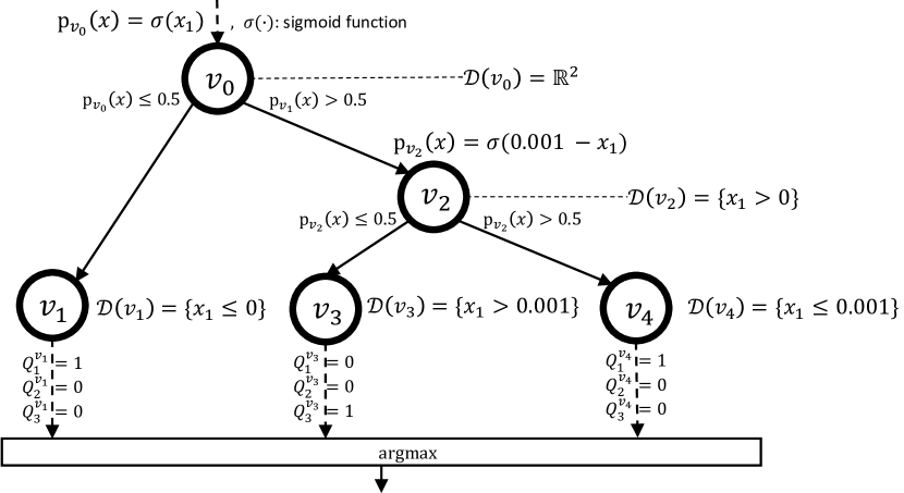
(b) Equivalent SDT for the NN in Fig. 1(a).

Figure 1: Example NN-to-SDT transformation.

Our results suggest that SDT transformation can be used to accelerate the verification of NN controllers in feedback control loops, with potential impact on applications where performance guarantees are critical but deep learning methods are the primary choice for control design.

Related Work. Distillation [7] has been used to transfer the knowledge and behavior of NN-based controllers to other models in an approximate, e.g., data-driven, or exact manner. Approximate distillation can be performed by training shallow NNs to mimic the behavior of state-of-the-art NNs using a teacher-student paradigm [8]. The distillation of SDTs from expert NNs was shown to lead to better performance than direct training of SDTs [7]. Furthermore, distillation has demonstrated success in reinforcement learning (RL) problems, where the DAGGER algorithm is used to transfer knowledge from Q-value NN models via simulation episodes [11]. Finally, distilling to SDTs has also been suggested to interpret the internal workings of black-box NNs [12].

In contrast, exact distillation has been proposed to transform feedforward NNs into simpler models while preserving equivalence [13, 14, 15]. Locally constant networks [13] and linear networks [14] have been introduced as intermediate representations to establish the equivalence between NNs and SDTs whose worst-case size scales exponentially in the maximum width of the NN hidden layers. Nguyen et al. [15] proposed transforming NNs with ReLUs into decision trees and then compressing the trees via a learning-based approach. As in previous approaches, our algorithm preserves equivalence with the SDTs. However, it also guarantees, without the need for compression, that the size of the tree scales polynomially in the width of the maximum hidden layer of the NN. Finally, we also provide quantitative evidence about the impact of the proposed transformations on the verifiability of the controllers.

II Preliminaries

We review key definitions for both neural networks and soft decision trees using Fig. 1 as an illustrative example. Throughout the paper, we use $A_{i,j}$ to denote the element in the $i$-th row and $j$-th column of matrix $A$, and $a_{i}$ or $(a)_{i}$ to denote the $i$-th element of vector $a$.

II-1 Neural Networks

Let $L$ denote the total number of layers in a NN, $N^{l}$ denote the width, or number of neurons in the $l$-th layer, and define $N:=(N^{1},\dots,N^{L})$. In Fig. 1(a), we have $L=3$, with a two-neuron input layer ($N^{1}=2$), a single-neuron hidden layer ($N^{2}=1$), and a three-neuron output layer ($N^{3}=3$), so that $N=(2,1,3)$. The nodes in layer $l$, with $l>1$, are fully connected to the previous layer. Edges and nodes are associated with weights and biases, denoted by $W^{l}$ and $B^{l}$, respectively, for $l\geq 2$. The output at each neuron is determined by its inputs using a feedforward function, defined below, and then passed through a rectified linear unit (ReLU) activation function.

Definition 1

(NN Layer Feedforward Function). Given input $x\in\mathbb{R}^{N^{l-1}}$, the feedforward function $f_{F}^{l}:\mathbb{R}^{N^{l-1}}\rightarrow\mathbb{R}^{N^{l}}$ maps $x$ to the output of layer $l\geq 2$, where the output of the $i$-th neuron in layer $l$ is defined as

$$(f_{F}^{l}(x))_{i}:=\sum_{i=1}^{N^{l-1}}W_{i,j}^{l}x_{j}+B_{i}^{l}.$$

We also recall the definition of characteristic function. Let $\alpha$ be the element-wise ReLU activation function, i.e., $\alpha(x)_{i}=\max\{x_{i},0\}$.

Definition 2

(NN Layer Characteristic Function). The characteristic function for layer $l$ of NN $\mathcal{N}$, $f_{\mathcal{N}}^{l}:\mathbb{R}^{N^{1}}\rightarrow\mathbb{R}^{N^{l}}$, is defined as

$$f_{\mathcal{N}}^{l}(x):=f_{F}^{l}\circ\alpha\circ f_{F}^{l-1}\circ\dots\circ f_{F}^{3}\circ\alpha\circ f_{F}^{2}(x).$$

Definition 3

(NN Characteristic Function). The characteristic function of NN $\mathcal{N}$, $f_{\mathcal{N}}:\mathbb{R}^{N^{1}}\rightarrow\mathbb{N}$, is defined as

$$f_{\mathcal{N}}(x):=\underset{i\in\{1,\dots,N^{L}\}}{\arg\max}\,\{(f_{\mathcal{N}}^{L}(x))_{i}:i\in\{1,\dots,N^{L}\}\}.$$

In Definition 3, we assume that when $\arg\max(.)$ is not a singleton, a deterministic tie-breaking procedure is used to select a single index.

Rules	Conditions	Computation of $p_{v}(x)$ or $Q^{v}$
1. Split based on ReLU	$\begin{array}[]{c}\exists\ i,l<L\ \text{s.t.}\ \mathcal{D}(v)\cap\{\mathcal{F}_{i}^{l}\llbracket v\rrbracket(x)\leq 0\}\not=\emptyset\;\wedge\\ \mathcal{D}(v)\cap\{\mathcal{F}_{i}^{l}\llbracket v\rrbracket(x)>0\}\not=\emptyset\end{array}$	$p_{v}(x)=\left\{\begin{array}[]{l}\sigma(\mathcal{F}_{i}^{l}\llbracket v\rrbracket(x))\\ \text{for}\ \min\,i,l\ \text{such that Rule~{}1 conditions hold}\\ \end{array}\right.$
2. Split based on output layer	$\begin{array}[]{c}\text{Rule~{}1 not satisfied and}\ \exists\ i_{1},i_{2}\ \text{s.t.}\\ \mathcal{D}(v)\cap\bigcap_{i^{\prime}\neq i_{1}}\{\mathcal{F}_{i_{1}}^{L}\llbracket v\rrbracket(x)\geq\mathcal{F}_{i^{\prime}}^{L}\llbracket v\rrbracket(x)\}\not=\emptyset\;\wedge\\ \mathcal{D}(v)\cap\bigcap_{i^{\prime}\neq i_{2}}\{\mathcal{F}_{i_{2}}^{L}\llbracket v\rrbracket(x)\geq\mathcal{F}_{i^{\prime}}^{L}\llbracket v\rrbracket(x)\}\not=\emptyset\end{array}$	$p_{v}(x)=\sigma(\mathcal{F}_{i_{1}}^{L}\llbracket v\rrbracket(x)-\mathcal{F}_{i_{2}}^{L}\llbracket v\rrbracket(x))$
3. Form leaf node	Neither Rule 1 nor Rule 2 satisfied	$Q_{i}^{v}=\left\{\begin{array}[]{ll}1&\text{if }i=\arg\max_{k}\{\mathcal{F}_{k}^{L}\llbracket v\rrbracket(x)\}\ \forall x\in\mathcal{D}(v)\\ 0&\text{otherwise}\\ \end{array}\right.$

TABLE I: Rules for constructing an SDT node $v$.

II-2 Soft Decision Trees

We consider a binary SDT [16, 12]. Let $\mathcal{I}_{\mathcal{S}}$ and $\mathcal{L}_{\mathcal{S}}$ denote the sets of inner and leaf nodes for an SDT $\mathcal{S}$ with input dimension $n$. Each inner node $v\in\mathcal{I}_{\mathcal{S}}$ is associated with weights $w^{v}\in\mathbb{R}^{n}$ and a bias term $b^{v}\in\mathbb{R}$. At node $v$, $w^{v}$ and $b^{v}$ are applied to input $x$. The resulting value is passed through an activation function $\sigma$, producing a scalar, $p_{v}(x)=\sigma(x^{\top}w^{v}+b^{v})$, which is compared to a threshold to determine whether to proceed to the left or right branch. In this paper, we use the sigmoid logistic activation function.

Each leaf node $v\in\mathcal{L}_{\mathcal{S}}$ is associated with a vector $Q^{v}$. In general, $Q^{v}$ is a distribution over possible output selections. In our SDTs, the elements of $Q^{v}$ will take values in $\{0,1\}$. Rather than learning the parameters $(w^{v},b^{v})$ or $Q^{v}$ for each node $v$ from data as in the literature [12], we derive these parameters via transformation of a reference NN. We denote the left and right child of an inner node $v$ as $l(v)$ and $r(v)$, respectively, and the parent of $v$ as $\rho(v)$. The root node of the SDT is $v_{0}$. We now define the SDT characteristic functions.

Definition 4

(SDT Node Characteristic Function). Let $\mathcal{S}$ be an SDT with input dimension $n$. Given input vectors $x\in\mathbb{R}^{n}$, the characteristic function of node $v$, $f_{\mathcal{S}}^{v}:\mathbb{R}^{n}\rightarrow\mathbb{N}$, is defined recursively as

$$f_{\mathcal{S}}^{v}(x)=\left\{\begin{array}[]{cl}\arg\max_{k}\{Q_{k}^{v}\},&\text{if }v\in\mathcal{L}_{\mathcal{S}},\\ f_{\mathcal{S}}^{l(v)}(x),&\text{if }v\in\mathcal{I}_{\mathcal{S}}\wedge p_{v}(x)\leq 0.5,\\ f_{\mathcal{S}}^{r(v)}(x),&\text{if }v\in\mathcal{I}_{\mathcal{S}}\wedge p_{v}(x)>0.5.\end{array}\right.$$

The output of each leaf node is then directly determined by a single path within the tree [12], rather than a weighted aggregation of all the potential tree paths [16].

Definition 5

(SDT Characteristic Function). The characteristic function of SDT $\mathcal{S}$ with input dimension $n$, $f_{\mathcal{S}}:\mathbb{R}^{n}\rightarrow\mathbb{N}$, is defined as $f_{\mathcal{S}}(x):=f_{\mathcal{S}}^{v_{0}}(x).$

Throughout this work, we assume that NNs and SDTs use the same deterministic argmax-based tie-breaking procedure. We further introduce the notation $\mathcal{D}(v)$ to represent the effective domain of an SDT node $v$, i.e., the set of all possible inputs arriving at $v$. The set $\mathcal{D}(v)$ can be computed recursively in a top-down manner from the root node as follows

$$\mathcal{D}(v)=\left\{\begin{array}[]{ll}\mathbb{R}^{n},&\text{if }v=v_{0},\\ \mathcal{D}(\rho(v))\;\cap&\text{if }v\not=v_{0}\;\wedge\\ \quad\{x|p_{\rho(v)}(x)\leq 0.5\},&\quad l(\rho(v))=v,\\ \mathcal{D}(\rho(v))\;\cap&\text{if }v\not=v_{0}\;\wedge\\ \quad\{x|p_{\rho(v)}(x)>0.5\},&\quad r(\rho(v))=v,\\ \end{array}\right.$$ (1)

where $n$ is the input dimension of the SDT.

For example, for the SDT in Fig. 1(b), the inputs $x=(x_{0},x_{1})^{\top}\in\mathbb{R}^{2}$ are processed starting from the root node $v_{0}$, where $\mathcal{D}(v_{0})=\mathbb{R}^{2}$. The input range related to node $v_{1}$ is $\mathcal{D}(v_{1})=\{x\in\mathbb{R}^{2}|x_{1}\leq 0\}$ and $v_{1}$ is reached only if $x_{1}\leq 0$. Similarly, node $v_{2}$ is reached when $x_{1}>0$, i.e., $\mathcal{D}(v_{2})=\{x\in\mathbb{R}^{2}|x_{1}>0\}$. In the remainder of the paper, we omit the reference to the underlying state-space in the expressions for the node input domains, when it is clear from the context, and simply write, e.g., $\mathcal{D}(v_{1})=\{x_{1}\leq 0\}$ and $\mathcal{D}(v_{2})=\{x_{1}>0\}$.

III Transformation from Neural Network to Decision Tree

We present an algorithm for constructing an SDT $\mathcal{S}_{\mathcal{N}}$ which is equivalent to a reference NN $\mathcal{N}$ in the sense that $f_{\mathcal{N}}(x)=f_{\mathcal{S}_{\mathcal{N}}}(x)$ for all inputs $x\in\mathbb{R}^{n}$. We outline the relation between fully connected NNs with ReLU activation and argmax output and SDTs based on our transformation in Fig. 1.

In the NN of Fig. 1(a), the output of the single neuron in layer 2 following the ReLU activation is

Carrying these two cases forward through the output layer $L=3$, we have

Thus, when $x_{1}\leq 0$, we have

$$f_{\mathcal{N}}(x)=\underset{i\in\{1,\dots,N^{L}\}}{\arg\max}\{(f_{\mathcal{N}}^{L}(x))_{i}\}=1,$$

while when $x_{1}>0$, we have

$$f_{\mathcal{N}}(x)=\begin{cases}1,&\text{if }x_{1}\leq 0.001,\\ 3,&\text{if }x_{1}>0.001,\end{cases}$$ (4)

assuming we take the lowest index to break ties.

Turning to the SDT in Fig. 1(b), we observe that (2) partitions the input space into two subsets based on the inner node’s ReLU activation. This is precisely the split that occurs at the root node $v_{0}$ of the SDT toward nodes $v_{1}$ and $v_{2}$. Then, (4) further splits one of these subsets based on the output layer values. This split occurs at $v_{2}$ to provide nodes $v_{3}$ and $v_{4}$. Finally, we have three regions where $f_{\mathcal{N}}(x)$ is constant, corresponding to leaf nodes $v_{1}$, $v_{3}$, and $v_{4}$ in Fig. 1(b).

As shown in (2)-(4) for subsets of the NN input space, based on the sequence of ReLU activations, $f^{L}_{\mathcal{N}}(x)$ is an affine function. Such subsets may be further partitioned based on the argmax operation. Therefore, the operation of fully connected NNs with ReLU activations and argmax output can be understood in terms of successive assignment of inputs from the state space to increasingly refined subspaces, which can be shown to consist of convex polyhedra [13]. Identification of SDT splits and leaf node assignments based on NN neuron activations and output layer outputs forms the core of our transformation technique, which we explain further in this section.

Assuming that the neural network depicted in Figure (1(a)) takes inputs $x=(x_{0},x_{1})^{\top}\in\mathbb{R}^{2}$, for node $v_{0}$ we have $\mathcal{D}(v_{0})=\mathbb{R}^{2}$. Since the pre-activation formula in layer $L$ is undefined for node $v_{0}$, i.e., $\mathcal{F}_{1}^{3}\llbracket v_{0}\rrbracket(x)=\mathcal{F}_{2}^{3}\llbracket v_{0}\rrbracket(x)=\bot$, Rule 1 should be applied. Specifically, using the first row of Equation (5), we can compute $\mathcal{F}_{1}^{2}\llbracket v_{0}\rrbracket(x)$ as $x_{1}$. As neither $\mathbb{R}^{2}\cap\{x_{1}>0\}$ nor $\mathbb{R}^{2}\cap\{x_{1}<0\}$ are empty sets, we create a split at $v_{0}$ by applying Rule 1 from Table I. This results in two child nodes, $l(v_{0})=v_{1}$ and $r(v_{0})=v_{2}$, and a splitting function $p_{v_{0}}(x)=\sigma(\mathcal{F}_{1}^{2}\llbracket v_{0}\rrbracket(x))$.

For node $v_{1}$, we first compute the pre-activation formulas and find that all pre-activation formulas at node $v_{1}$ are not undefined and only the first output neuron can produce the maximum output. Hence, Rule 3 should be applied. Specifically, using Equation (1), we find that $\mathcal{D}(v_{1})=\{x_{1}\leq 0\}$. Since $\mathcal{F}_{1}^{2}\llbracket v_{1}\rrbracket$ is not undefined and $\mathcal{D}(v_{1})\cap\{\mathcal{F}_{1}^{2}\llbracket v_{1}\rrbracket(x)>0\}$ is an empty set, we can use the second row of Equation (6) to set $\overline{\mathcal{F}_{1}^{2}\llbracket v_{1}\rrbracket}(x)=0$. Moving on to $l=3$ in Equation (5), we find that $\mathcal{F}_{i}^{3}\llbracket x\rrbracket=B^{3}_{i}$ for $i\in\{1,2,3\}$, which implies that $\mathcal{F}_{1}^{3}\llbracket v_{1}\rrbracket(x)=0.001$, $\mathcal{F}_{2}^{3}\llbracket v_{1}\rrbracket(x)=0$, and $\mathcal{F}_{3}^{3}\llbracket v_{1}\rrbracket(x)=0$. Since Rule 2 cannot be applied, we use Rule 3 to set $Q_{1}^{v_{1}}(x)=1$ and $Q_{2}^{v_{1}}(x)=Q_{3}^{v_{1}}(x)=0$.

Moving on to node $v_{2}$, we find that although all pre-activation formulas are not undefined, both the first and second output neurons can produce the maximum output. Specifically, Rule 1 cannot be satisfied since $\mathcal{D}(v_{2})\cap\{\mathcal{F}_{1}^{2}\llbracket v_{2}\rrbracket(x)\leq 0\}$ is empty. However, both $\mathcal{D}(v_{2})\cap\{\mathcal{F}_{1}^{3}\llbracket v_{2}\rrbracket(x)<\mathcal{F}_{3}^{3}\llbracket v_{2}\rrbracket(x)\}=\{0.001<x_{1}\}$ and $\mathcal{D}(v_{2})\cap\{\mathcal{F}_{1}^{3}\llbracket v_{2}\rrbracket(x)\geq\mathcal{F}_{3}^{3}\llbracket v_{2}\rrbracket(x)\}=\{0<x_{1}\leq 0.001\}$ are non-empty. Therefore, we use Rule 2 to set $p_{v_{2}}(x)$ as $\sigma(\mathcal{F}_{1}^{3}\llbracket v_{2}\rrbracket(x)-\mathcal{F}_{3}^{3}\llbracket v_{2}\rrbracket(x))$. We repeat this process for nodes $v_{3}$ and $v_{4}$ and transform the example NN in Figure (1(a)) to the SDT in Figure (1(b)).

To demonstrate the advantages of SDT controllers over NN controllers, we compare the formulations of an example NN $\mathcal{N}$ and an equivalent SDT $\mathcal{S}_{\mathcal{N}}$ in Figures (1). The formulations of $f_{\mathcal{N}}(x)$ and $f_{\mathcal{S}_{\mathcal{N}}}(x)$ are given by

$$\begin{split}&(z\geq x_{1})\wedge(z\geq 0)\wedge[(z=0)\vee(z=x_{1})]\\ &\qquad\wedge[(u=3)\vee(z\leq 0.001)]\wedge[(u=1)\vee(z>0.001)],\end{split}$$

where $z$ is the variable for the only inner neuron, and

$$[(u=3)\vee(x_{1}\leq 0.001)]\wedge[(u=1)\vee(x_{1}>0.001)],$$

respectively. In NNs, the output $f_{\mathcal{N}}(x)$ becomes more complex and increases the number of internal variables as the number of layers increases, while in SDTs, each node $v$ outputs a scalar $p_{v}(x)$ derived from a single weighting of the input. Thus, the relation between input $x$ and SDT output $f_{\mathcal{S}_{\mathcal{N}}}(x)$ is more straightforward, leading to a comparatively simple relation that can significantly reduce verification time.

III-A Pre and Post-Activation Formulas

We establish the relationship between $\mathcal{N}$ and $\mathcal{S}_{\mathcal{N}}$ by first introducing, for each node $v$, a pre-activation function $\mathcal{F}_{i}^{l}\llbracket v\rrbracket\,:\,\mathcal{D}(v)\to\mathbb{R}$ and a post-activation function $\overline{\mathcal{F}_{i}^{l}\llbracket v\rrbracket}\,:\,\mathcal{D}(v)\to\mathbb{R}$. The pre-activation function provides the output of the $i$-th neuron in the $l$-th layer of $\mathcal{N}$ as a function of the input in $\mathcal{D}(v)$ prior to the ReLU. The post-activation function gives the neuron output after the ReLU. The pre-activation functions for node $v$ are defined for $l=2,\dots,L$ and $i=1,\dots,N^{l}$ as

Here, $\bot$ denotes an undefined value. The post-activation functions for node $v$ are defined for $l=2,\dots,L-1$ and $i=1,\dots,N^{l}$ as

$$\begin{split}\overline{\mathcal{F}_{i}^{l}\llbracket v\rrbracket}(x)=\begin{cases}\mathcal{F}_{i}^{l}\llbracket v\rrbracket(x),&\text{if }\mathcal{F}_{i}^{l}\llbracket v\rrbracket\not=\bot\;\wedge\\ &\quad\mathcal{D}(v)\cap\{\mathcal{F}_{i}^{l}\llbracket v\rrbracket(x)\leq 0\}=\emptyset,\\ 0,&\text{if }\mathcal{F}_{i}^{l}\llbracket v\rrbracket\not=\bot\;\wedge\\ &\quad\mathcal{D}(v)\cap\{\mathcal{F}_{i}^{l}\llbracket v\rrbracket(x)>0\}=\emptyset,\\ \bot,&\text{otherwise}.\end{cases}\end{split}$$ (6)

We define $\mathcal{F}^{l}\llbracket v\rrbracket:=(\mathcal{F}_{1}^{l}\llbracket v\rrbracket,\dots,\mathcal{F}_{N^{l}}^{l}\llbracket v\rrbracket)^{\top}$ and $\overline{\mathcal{F}^{l}\llbracket v\rrbracket}$ similarly for all $l=2,\dots,L$. The pre-activation formulas play a crucial role in determining the pre-threshold branching functions $p_{v}$ at each inner node $v$ of $\mathcal{S}$.

III-B SDT Split and Leaf Formation Rules

We construct the branches of $\mathcal{S}_{\mathcal{N}}$ based on the rules in Table I. By starting with the root node $v_{0}$, for each node $v$ in $\mathcal{S}_{\mathcal{N}}$, we use Table I to obtain $p_{v}(x)$ or $Q^{v}$ in a top-down fashion from root to leaves, as further explained below.

Rule 1. If there exists a neuron $i$ in layer $l$ of $\mathcal{N}$ such that $D_{0}:=\mathcal{D}(v)\cap\{\alpha(\mathcal{F}_{i}^{l}\llbracket v\rrbracket(x))=0\}\neq\emptyset$ and $D_{1}:=\mathcal{D}(v)\cap\{\alpha(\mathcal{F}_{i}^{l}\llbracket v\rrbracket(x))>0\}\neq\emptyset$ hold, we form a split at node $v$ in $\mathcal{S}_{\mathcal{N}}$. $\mathcal{D}(v)$ is then partitioned along the hyperplane $\mathcal{F}_{i}^{l}\llbracket v\rrbracket(x)=0$, with $\mathcal{D}(l(v))=D_{0}$ and $\mathcal{D}(r(v))=D_{1}$. For example, for node $v_{0}$ in Fig. 1(b), we create a split at $v_{0}$ with $p_{v_{0}}(x)=\sigma(\mathcal{F}_{1}^{2}\llbracket v_{0}\rrbracket(x))$.

Rule 2. Suppose no partitions can be found for $\mathcal{D}(v)$ based on the ReLUs according to Rule 1. Then, $\mathcal{D}(v)$ may be further partitioned based on the output layer values. If there exist $i_{1}$ and $i_{2}$ and sets $D_{i_{1}}:=\{x\in\mathcal{D}(v)|\arg\max_{i}\{(\mathcal{F}^{L}\llbracket v\rrbracket(x))_{i}\}=i_{1}\}\neq\emptyset$ and $D_{i_{2}}:=\{x\in\mathcal{D}(v)|\arg\max_{i}\{(\mathcal{F}^{L}\llbracket v\rrbracket(x))_{i}\}=i_{2}\}\neq\emptyset$, we form a split at node $v$. $\mathcal{D}(v)$ is then partitioned along the hyperplane $\mathcal{F}_{i_{2}}^{L}\llbracket v\rrbracket(x)-\mathcal{F}_{i_{1}}^{L}\llbracket v\rrbracket(x)=0$, giving $D_{i_{1}}\subseteq\mathcal{D}(l(v))$ and $D_{i_{2}}\subseteq\mathcal{D}(r(v))$. For example, for node $v_{2}$ in Fig. 1(b), we create a split at $v_{2}$ and set $p_{v_{2}}(x)$ as $\sigma(\mathcal{F}_{1}^{3}\llbracket v_{2}\rrbracket(x)-\mathcal{F}_{3}^{3}\llbracket v_{2}\rrbracket(x))$.

Rule 3. If neither Rule 1 nor Rule 2 can be applied to further partition $\mathcal{D}(v)$, then the index of the neuron with the maximum output at layer $L$, i.e., the outcome of the $\arg\max$ operator remains constant over the entire set $\mathcal{D}(v)$. We then declare $v$ as a leaf node, setting $Q^{v}_{i}=1$ for the neuron index corresponding to the largest output, and $0$ otherwise. For example, for node $v_{1}$ in Fig. 1(b) we set $Q_{1}^{v_{1}}(x)=1$ and $Q_{2}^{v_{1}}(x)=Q_{3}^{v_{1}}(x)=0$.

The conditions above, such as non-emptiness of $\mathcal{D}(v)\cap\{\alpha(\mathcal{F}_{i}^{l}\llbracket v\rrbracket(x))=0\}$ in Rule 1, can be formulated and efficiently solved in terms of feasibility problems for linear programs.

III-C Transformation Procedure

We construct $\mathcal{S}_{\mathcal{N}}$ by starting with the root node $v_{0}$ and building the binary tree downwards. We first construct the left-hand branches until a leaf node is discovered, from which we backtrack the tree to define the unexplored right branches. A recursive method implementing this procedure is presented in Algorithm 1. The transformation procedure effectively identifies a partition of the input space according to the domains associated with the leaf nodes of the SDT. Within these sets, the neural network characteristic function $f_{\mathcal{N}}$ is constant, and due to our choice of $Q^{v}$ at each leaf node $v$, we have that $f_{\mathcal{N}}(x)=f_{\mathcal{S}_{\mathcal{N}}}(x)$ over $\mathcal{D}(v)$. Taking a union over the SDT partitions, we establish the equivalence of $\mathcal{N}$ and $\mathcal{S}_{\mathcal{N}}$ in Theorem 1. As detailed in Appendix -A, Theorem 1 can be proved by induction on layer $l$ to show that $\mathcal{F}^{L}\llbracket v\rrbracket(x)=f^{L}_{\mathcal{N}}(x)$ holds for leaf nodes $v\in\mathcal{L}_{\mathcal{S}_{\mathcal{N}}}$.

Theorem 1

For a given NN $\mathcal{N}$ and its SDT transformation $\mathcal{S}_{\mathcal{N}}$ using Algorithm 1 with input space $\mathbb{R}^{n}$, the corresponding characteristic functions are pointwise equal, i.e., $f_{\mathcal{N}}(x)=f_{\mathcal{S}_{\mathcal{N}}}(x)$ for all $x\in\mathbb{R}^{n}.$

Differently from previous algorithms in the literature [15, 13, 14], our algorithm only generates essential branches during the creation of the SDT. Given the NN input and output layer sizes and the number of hidden layers, the SDT size scales polynomially in the maximum hidden layer width. The size complexity of $\mathcal{S}_{\mathcal{N}}$ in terms of the number of nodes is stated in Theorem 2, whose proof, provided in Appendix -B, is based on the upper bound on the number of piecewise affine regions achievable with ReLU NNs [17].

Theorem 2

Let $\mathcal{N}$ be a NN and $\mathcal{S}_{\mathcal{N}}$ the SDT resulting from the application of Algorithm 1 to $\mathcal{N}$. Denote the number of nodes in $\mathcal{S}_{\mathcal{N}}$ by $|\mathcal{S}_{\mathcal{N}}|$. Then, we obtain

$$|\mathcal{S}_{\mathcal{N}}|=O\left(\prod_{l=2}^{L-1}\frac{(N^{l})^{(N^{1})}}{(N^{1})!}2^{N^{L}}\right)=O\left(\frac{2^{N^{L}}}{(N^{1}!)^{L}}\overline{l}^{N^{1}L}\right),$$

where $\overline{l}:=\max_{l\in\{2,\dots,L-1\}}N^{l}$.

Algorithm 1 SDT Transformation $\mathcal{T}$(.)

1:Global Variables: NN parameters $L$, $\{N^{l}\}_{l=1}^{L}$, $\{W^{l},b^{l}\}_{l=2}^{L}$

2:Input: $v$

3:Compute $\mathcal{D}(v)$ via (1)

4:for $l=2,\dots,L$ do

5:    for $i=1,\dots,N^{l}$ do

6:         Compute $\mathcal{F}^{l}_{i}\llbracket v\rrbracket$, $\overline{\mathcal{F}^{l}_{i}\llbracket v\rrbracket}$ via (5), (6)     

7:if $\exists\ i,l$ s.t. ($\mathcal{D}(v),\mathcal{F}^{l}_{i}\llbracket v\rrbracket$) satisfy Rule 1 then

8:    $p_{v}(x)=\sigma(\mathcal{F}_{i}^{l}\llbracket v\rrbracket(x))$, create $l(v)$, $r(v)$

9:    $\mathcal{T}(l(v))$ $\triangleright$ Recursion

10:    $\mathcal{T}(r(v))$

11:else if $\exists\ i_{1},i_{2}$ s.t. ($\mathcal{D}(v),\mathcal{F}^{L}_{i_{1}},\llbracket v\rrbracket,\mathcal{F}^{L}_{i_{2}},\llbracket v\rrbracket$) satisfy Rule 2 then

12:    $p_{v}(x)=\sigma(\mathcal{F}_{i_{1}}^{L}\llbracket v\rrbracket(x)-\mathcal{F}_{i_{2}}^{L}\llbracket v\rrbracket(x))$, create $l(v)$, $r(v)$.

13:    $\mathcal{T}(l(v))$ $\triangleright$ Recursion

14:    $\mathcal{T}(r(v))$

15:else

16:    $Q_{i}^{v}=$ $\left\{\begin{array}[]{ll}1&\text{if }i=\arg\max_{k}\{\mathcal{F}_{k}^{L}\llbracket v\rrbracket\},\forall x\in\mathcal{D}(v)\\ 0&\text{otherwise}\\ \end{array}\right.$

IV Verification Formulation

We describe the verification problems that we solve to evaluate the impact of the proposed transformation. We consider closed-loop controlled dynamical systems with state and action spaces $\mathcal{X}$ and $\mathcal{U}$, respectively, and dynamics $h\,:\,\mathcal{X}\times\mathcal{U}\to\mathcal{X}$. Let $\pi\,:\,\mathcal{X}\to\mathcal{U}$ denote a time-invariant Markovian policy (controller) mapping states to actions. Given a system dynamics $h$, an initial set $\mathcal{X}_{i}$, and goal set $\mathcal{X}_{g}$, we wish to determine whether $\mathcal{X}_{g}$ is reachable in finite horizon $T$ for all initial states $x_{0}\in\mathcal{X}_{i}$, under $h$ and policy $\pi$. If so, we say that the specification $(\mathcal{X}_{i},\mathcal{X}_{g},T)$ is verified for $\pi$. In this context, we consider two verification approaches.

Problem 1

(One-Shot Verification). We “unroll” the system dynamics at time instant $t\in\{0,\ldots,T\}$ and encode the verification problem to a satisfiability modulo theory (SMT) problem [18] using the bounded model checking approach [19]. Verification of $(\mathcal{X}_{i},\mathcal{X}_{g},T)$ for a policy $\pi$ is then equivalent to showing that the following formula is not satisfiable:

If $\phi_{1}(\pi)$ is false, then $\pi$ is guaranteed to drive the system from any $x_{0}\in\mathcal{X}_{i}$ to $\mathcal{X}_{g}$ within the finite horizon $T$.

We observe that (7) requires encoding $T$ replicas of the NN (policy $\pi$) in the control loop, which can make the SMT problem intractable due to its computational complexity. Therefore, we also consider an alternative verification approach via reachability analysis. In particular, we adopt a recursive reachability analysis [20], where we use the $s$-step unrolled dynamics, with $s\ll T$, to compute an over-approximation of the $s$-step reachable set in terms of a rectangle.

Problem 2

(Recursive Reachability Analysis (RRA)). We fix a step parameter $s$ and recursively compute reachable sets $\mathcal{R}_{t}$, where $t=ms$ for $m\in\mathbb{N}$. Given a system dynamics $h$, policy $\pi$ and step parameter $s$, we encode the reachable set at time $t$ as the SMT formula

$$\begin{split}&\mathcal{R}_{t}(\pi)=\bigg{\{}x\bigg{|}x=x_{t}\wedge(\mathcal{R}_{t-s})\;\wedge\\ &\quad\quad\quad\quad\bigwedge_{k=t-s}^{t-1}(x_{k+1}=h(x_{k},u_{k}))\wedge(u_{k}=\pi(x_{k}))\bigg{\}}.\\ \end{split}$$ (8)

By setting $\mathcal{R}_{0}=\mathcal{X}_{i}$, we can verify the specification $(\mathcal{X}_{i},\mathcal{X}_{g},T)$ by checking satisfaction of the following SMT formula

$$\phi_{\text{RRA}}(\pi):=(\mathcal{X}_{i})\wedge(\overline{\mathcal{X}_{g}})\wedge\bigcup_{m=1}^{\lfloor T/s\rfloor}\mathcal{R}_{ms}(\pi).$$

While RRA may yield overly conservative reachable sets due to error propagation, it is often more tractable than one-shot verification, since it decomposes the overall reachability problem into a set of smaller sub-problems, each having a finite horizon of $s$ and encoding the NN policy only $s$ times, with $s\ll T$.

V Case Studies

Environment	$\mathfrak{i}_{l}$	$\mathfrak{i}_{u}$	$\mathfrak{g}$
MountainCar	$-0.11$	$-0.1$	$0.5$
CartPole	$-0.1$	N/A	$\pi/15$

TABLE II: Hyperparameters in OpenAI Gym.

V-A The Environments

V-A1 MountainCar-v0

In the MountainCar control task, an underpowered car needs to reach the top of a hill starting from a valley within a fixed time horizon $T$ [21]. The state vector $x_{t}\in\mathbb{R}^{2}$ comprises the car’s position $x_{t,0}$ and horizontal velocity $x_{t,1}$ at time step $t$, while the input $u_{t}\in\{-1,0,1\}$ represent the car’s acceleration action, either left (L), idle (I), or right (R), respectively. The system dynamics are given in Appendix -C.

While the reference NNs are trained to reach the top of the hill $(x\geq\mathfrak{g})$ in the minimum number of steps, we seek to verify whether a given controller will reach the goal state within $T$ steps, starting from any point in an initial interval. Our specification $(\mathcal{X}_{i},\mathcal{X}_{g},T)$ is given by

$$\begin{split}&\mathcal{X}_{i}=\{x_{0}\in[\mathfrak{i}_{l},\mathfrak{i}_{u}],x_{1}=0\},\,\,\mathcal{X}_{g}=\bigcup_{t=0}^{T}\{x_{t,0}\geq\mathfrak{g}\},\end{split}$$

where $\mathfrak{i}_{l}$, $\mathfrak{i}_{u}$, and $\mathfrak{g}$ are parameters.

V-A2 CartPole-v1

In the CartPole control task [22], a pole is attached to a cart moving along a frictionless track, to be balanced upright for as long as possible within a fixed horizon $T$. The state vector $x_{t}\in\mathbb{R}^{4}$ consists of the cart position $x_{t,0}$, the cart velocity $x_{t,1}$, the pole angle $x_{t,2}=\theta_{t}$, and the pole angular velocity $x_{t,3}$ at time step $t$. The input $u_{t}\in\{0,1\}$ denotes the acceleration of the cart to the left or right. The system dynamics are given in Appendix -D.

We seek to verify that the pole is balanced upright within tolerance $\mathfrak{g}$ at the end of horizon $T$, starting from a range of initial cart positions and pole angles. With $\mathfrak{i}_{l}$, $\mathfrak{g}$ as parameters, our specification $(\mathcal{X}_{i},\mathcal{X}_{g},T)$ is given by

$$\begin{split}&\mathcal{X}_{i}=\{x_{0,0}\in[\mathfrak{i}_{l},0],x_{0,2}\in[\mathfrak{i}_{l},0],x_{0,1}=x_{0,3}=0\}\\ &\mathcal{X}_{g}=\{|x_{T,2}|\geq\mathfrak{g}\}.\end{split}$$

V-B Evaluation Results

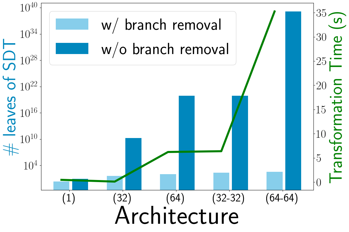
(a) MountainCar

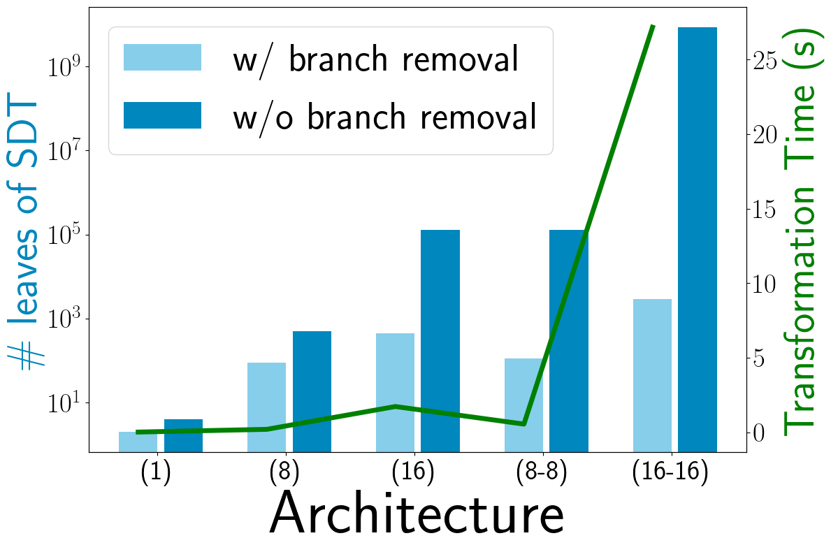
(b) CartPole

Figure 2: Transformation time and size of the transformed SDT.

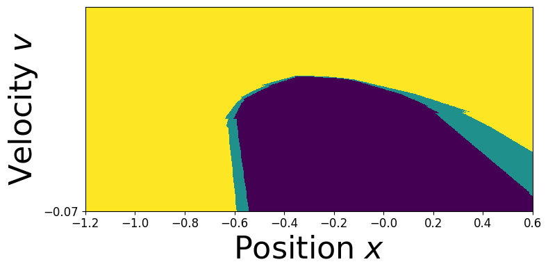
(a) $N=(2,64,3)$

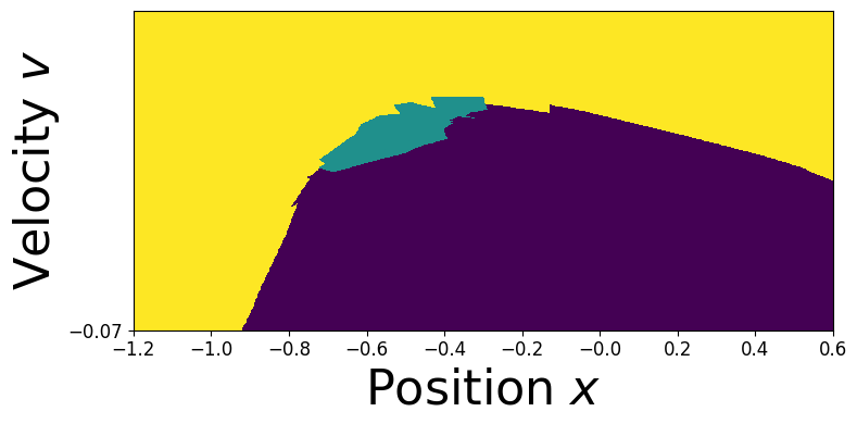
(b) $N=(2,64,64,3)$

Figure 3: MountainCar NN policies, L ( ), I ( ), R ( ).

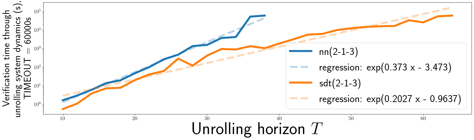
Figure 4: Comparison of MountainCar NN and SDT controller one-shot verification times.

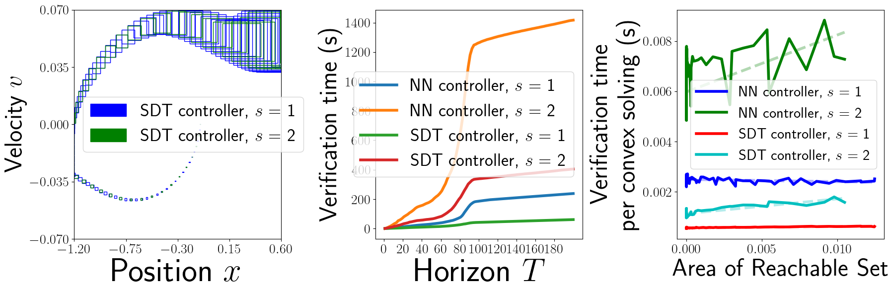
(a) Reachable sets and verification time for MountainCar NN with $N=(2,32,32,3)$.

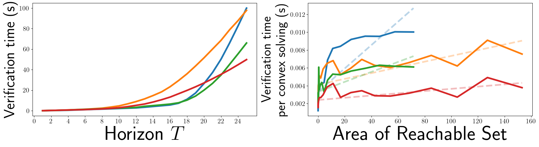
(b) Verification time for CartPole NN ( ) and SDT ( ) with $N=(4,8,2)$, and NN ( ) and SDT ( ) with $N=(4,8,8,2)$.

Figure 5: Recursive Reachability Analysis results.

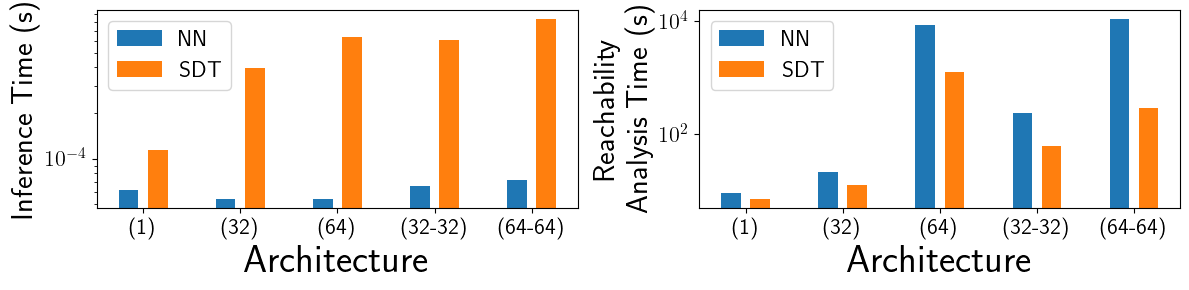
(a) MountainCar.

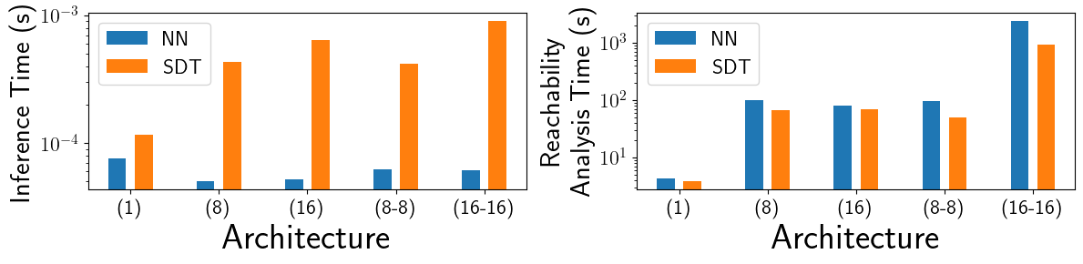
(b) CartPole.

Figure 6: Inference and RRA runtimes for NN and SDT controllers. For RRA, $T=200$ for MountainCar and $T=25$ for CartPole.

We adopt the problem setups available in the open-source package OpenAI Gym [10] and the parameters in Table II. We train NN controllers for $1\times 10^{7}$ steps. Fig. 2 illustrates the transformation time and the number of leaves of the SDT for each NN controller. We also display the estimated number of leaves under a naïve transformation method that generates a split at every node for every neuron in every layer, denoted by “w/o branch removal”. This value signifies the percentage reduction in size achieved by our transformation. As shown in Fig. 2, the percentage of size reduction for the SDT increases with the number of NN layers. Furthermore, the size of the transformed SDT for the CartPole problem increases faster than for the MountainCar problem, which can be attributed to the difference in $N^{1}=|x_{t}|$. Nevertheless, we were able to transform all the controllers in less than $60$ s.

Fig. 3 plots the policies and SDT leaf node partitions for example MountainCar controllers. Note that constant action state-space regions become more complex as the depth of the NN increases.

All SMT problems in our experiments are solved using an in-house implementation of a satisfiability modulo convex programming (SMC) solver [23], which integrates the Z3 satisfiability (SAT) solver [24] with Gurobi [25]. For the one-shot verification approach, Fig. 4 shows a comparison of the verification times for $\mathcal{N}$ with $N=(2,1,3)$ and $\mathcal{S}_{\mathcal{N}}$ with three leaf nodes in the MountainCar problem. The NN verification time increases significantly compared to the equivalent SDT. However, verification takes more than 60000 seconds for $\mathcal{N}$ when $T>38$ and for $\mathcal{S}_{\mathcal{N}}$ when $T>64$. For the CartPole problem, all controllers fail to solve the verification problem (7) within 60000 seconds for $T>10$.

To assess the efficiency of RRA for NN and SDT controllers, we measured runtimes both for individual reachability set determination as well as overall verification time. Fig. 5(a) plots the reachable sets, along with overall verification and reachable set generation times for an example MountainCar controller with $s\in\{1,2\}$ in (8). Fig. 5(b) plots verification and reachable set generation times for a collection of CartPole controllers with $s=1$ in (8). As shown, RRA verification becomes more efficient using the equivalent SDT controllers, rather than the reference NNs.

Fig. 6 compares the average inference and overall RRA verification times for a collection of NN and equivalent SDT controllers. We set $T=200$ for the MountainCar problem and $T=25$ for the CartPole problem. While the inference time for the SDT increases with the number of layers in NN, our results show that the transformed SDT controller accelerates verification for the MountainCar problem by up to $21\times$ and for the CartPole problem by up to $2\times$. Moreover, the larger the number of layers in the NN, the larger the difference between runtime for NN verification and runtime for SDT verification.

VI Conclusion

We proposed a cost-effective algorithm to construct equivalent SDT controllers from any discrete-output argmax-based NN controller. Empirical evaluation of formal verification tasks performed on two benchmark OpenAI Gym environments shows a significant reduction in verification times for SDT controllers. Future work includes experimenting with more sophisticated RL environments and performing more extensive comparisons with state-of-the-art verification tools.

-A Proof of Theorem 1

Before proving the main theorem, we establish the following lemma to prove the transformed SDT is not undefined.

Lemma 1

For all inner nodes $v$ of $\mathcal{S}_{\mathcal{N}}$ $p_{v}\neq\sigma(\mathrm{undef}).$

Proof:

Note that the assignment $p_{v}=\sigma(\mathrm{undef})$, can only occur for a node $v$ satisfying Rule 1 or Rule 2.

If Rule 1 applies, let $p_{v}=\sigma(\mathcal{F}_{i}^{l}\llbracket v\rrbracket)$ with $\mathcal{F}_{i}^{l}\llbracket v\rrbracket=\bot$. Then, due to (5), there must also exist $l^{\prime}<l$ and $i^{\prime}$ such that $\mathcal{F}_{i^{\prime}}^{l^{\prime}}\llbracket v\rrbracket$ is defined but $\overline{\mathcal{F}_{i^{\prime}}^{l^{\prime}}\llbracket v\rrbracket}$ is not. By the third row of (6), both $\mathcal{D}(v)\cap\{\mathcal{F}_{i^{\prime}}^{l^{\prime}}\llbracket v\rrbracket(x)\leq 0\}$ and $\mathcal{D}(v)\cap\{\mathcal{F}_{i^{\prime}}^{l^{\prime}}\llbracket v\rrbracket(x)>0\}$ are non-empty. In this case Rule 1 would assign $p_{v}=\sigma(\mathcal{F}_{i^{\prime}}^{l^{\prime}}\llbracket v\rrbracket)$, which contradicts our assumption that $p_{v}=\sigma(\mathcal{F}_{i}^{l}\llbracket v\rrbracket)$.

If Rule 2 applies, then $p_{v}=\sigma(\mathcal{F}_{i_{1}}^{L}\llbracket v\rrbracket-\mathcal{F}_{i_{2}}^{L}\llbracket v\rrbracket)=\sigma(\bot)$, and for some $i\in\{i_{1},i_{2}\}$, we have $\mathcal{F}_{i}^{L}\llbracket v\rrbracket=\bot$. We can then take $l=L$ and repeat the argument for the Rule 1 case to arrive at a contradiction in the assignment of $p_{v}=\sigma(\mathcal{F}_{i_{1}}^{L}\llbracket v\rrbracket-\mathcal{F}_{i_{2}}^{L}\llbracket v\rrbracket)$. ∎

We now establish the following lemma to prove our main theorem.

Lemma 2

Given a NN $\mathcal{N}$, and a its SDT transformation $\mathcal{S}_{\mathcal{N}}$, let $\mathcal{L}$ denote the set of leaf nodes of $\mathcal{S}_{\mathcal{N}}$. Then, for $v\in\mathcal{L}$ and $x\in\mathcal{D}(v)$, we have

$$\mathcal{F}^{L}\llbracket v\rrbracket(x)=f^{L}_{\mathcal{N}}(x).$$

Proof:

We prove this result via induction on $l=2,\dots,L$. For $l=2$, each node $v$ and $x\in\mathcal{D}(v)$, (5) gives

$$\mathcal{F}^{2}\llbracket v\rrbracket(x)=W^{2}x+B^{2}=f_{\mathcal{N}}^{2}(x).$$

For the induction step, assume that $(f_{\mathcal{N}}^{l}(x))_{i}=\mathcal{F}_{i}^{l}\llbracket v\rrbracket(x)$ for all $i\in\{1,2,\dots,N^{l}\}$. Then, by Definition 1, for $i\leq N^{l+1}$ we have for all $x\in\mathcal{D}(v)$

$$(f_{\mathcal{N}}^{l+1}(x))_{i}=\sum_{j=0}^{N^{l}}(W^{l+1}_{i,j}\alpha(\mathcal{F}_{j}^{l}\llbracket v\rrbracket(x)))+B_{i}^{l+1}.$$ (9)

We consider two cases. First, if $\mathcal{D}(v)\cap\{\mathcal{F}_{j}^{l}\llbracket v\rrbracket(x)\leq 0\}$ is empty, then $\mathcal{F}_{j}^{l}\llbracket v\rrbracket(x)>0$ for all $x\in\mathcal{D}(v)$, which implies

$$\alpha(\mathcal{F}_{j}^{l}\llbracket v\rrbracket(x))=\mathcal{F}_{j}^{l}\llbracket v\rrbracket(x)=\overline{\mathcal{F}_{j}^{l}\llbracket v\rrbracket}(x).$$ (10)

Second, if $\mathcal{D}(v)\cap\{\mathcal{F}_{j}^{l}\llbracket v\rrbracket(x)>0\}$ is empty, then for all $x\in\mathcal{D}(v)$, we have $\mathcal{F}_{j}^{l}\llbracket v\rrbracket(x)\leq 0$, which implies

$$\alpha(\mathcal{F}_{j}^{l}\llbracket v\rrbracket(x))=0=\overline{\mathcal{F}_{j}^{l}\llbracket v\rrbracket}(x).$$ (11)

Therefore, combining (9)-(11), and (5), we have

$$(f^{l+1}_{\mathcal{N}}(x))_{i}=\sum_{j=0}^{N^{l}}(W^{l+1}_{i,j}\overline{\mathcal{F}_{j}^{l}\llbracket v\rrbracket(x)})+B_{i}^{l+1}=\mathcal{F}_{i}^{l+1}\llbracket v\rrbracket(x).$$

∎

By construction, the leaf node regions $\mathcal{D}(v)$ for $v\in\mathcal{L}$ for a partition of the input space $\mathbb{R}^{n}$. Therefore, using Lemma 2, we may write

$$f^{L}_{\mathcal{N}}(x)=\sum_{v\in\mathcal{L}}\mathds{1}_{\{x\in\mathcal{D}(v)\}}\mathcal{F}^{l}\llbracket v\rrbracket(x)=\mathcal{F}^{l}\llbracket v_{x}\rrbracket(x),$$ (12)

where $v_{x}$ is the leaf node to which $x$ is assigned, i.e., $x\in\mathcal{D}(v_{x})$. Taking argmax over the left and right of (12), and using the same tie-breaking procedure for both $\mathcal{N}$ and $\mathcal{S}_{\mathcal{N}}$, we have

$$\begin{split}&f_{\mathcal{N}}(x)=\underset{i\in\{1,\dots,N^{L}\}}{\arg\max}\{(f^{L}_{\mathcal{N}}(x))_{i}\}=\underset{i\in\{1,\dots,N^{L}\}}{\arg\max}\{\mathcal{F}_{i}^{l}\llbracket v_{x}\rrbracket(x)\}\\ &\quad=f_{\mathcal{S}_{\mathcal{N}}}(x).\end{split}$$

∎

-B Proof of Theorem 2

This section presents the proof of Theorem 2, which compares the complexity of a neural network with that of the transformed SDT. To facilitate the proof, we define $B(x,\delta)$ as the Euclidean ball of radius $\delta$ centered at $x\in\mathbb{R}^{n}$, where $\delta>0$. We then recall the definition of a hyperplane arrangement, region of a hyperplane arrangement, and recall a bound on the number of regions of a hyperplane arrangement established in [26].

Definition 6

(Hyperplane Arrangement) Let $\mathcal{A}$ be a set of affine functions where each $f\in\mathcal{A}\,:\,\mathbb{R}^{n}\to\mathbb{R}$. Then $\mathcal{H}=\bigcup_{f\in\mathcal{A}}\{x|f(x)=0\}$ is an arrangement of hyperplanes in dimension $n$.

Definition 7

(Region of a Hyperplane Arrangement) Let $\mathcal{H}$ be an arrangement of $N$ hyperplanes in $n$-dimensional space, defined by a set of affine functions $\mathcal{A}$. A non-empty open subset $R\subseteq\mathbb{R}^{n}$ is called an $n$-dimensional region of $\mathcal{H}$ if $R=\bigcap_{f\in\mathcal{A}}\{x|f(x)\bowtie 0\}$, where $\bowtie$ is either $<$ or $>$ and there exists $\delta>0$ such that $B(x,\delta)\subseteq R$. The set of all regions of $\mathcal{A}$ is denoted as $\mathfrak{R}_{\mathcal{H}}$.

Theorem 3

(Theorem 1 [26]) Let $\mathcal{H}$ be an arrangement of $N$ hyperplanes in dimension $n$, defined by a set of affine functions $\mathcal{A}$. The number of regions of $\mathcal{H}$, denoted by $|\mathfrak{R}_{\mathcal{H}}|$, is at most $\sum_{k=0}^{n}\binom{N}{k}$, which is bounded by $O(N^{n}/n!)$.

We introduce a notation $\mathcal{V}_{l}(v)$ to denote the set of nodes $v^{\prime}$ such that $v^{\prime}$ is a successor of $v$ and $p_{\pi(v^{\prime})}(x)$ is derived via Rule 1 at layer $l$, while $p_{v^{\prime}}(x)$ is not:

$$\begin{split}&\mathcal{V}_{l}(v)=\{v^{\prime}\mid v^{\prime}\text{ is a successor node of }v,\\ &\quad\,\,p_{\pi(v^{\prime})}(x)=\sigma(\mathcal{F}_{i}^{l}\llbracket\pi(v^{\prime})\rrbracket(x)),p_{v^{\prime}}(x)\neq\sigma(\mathcal{F}_{i^{\prime}}^{l}\llbracket v^{\prime}\rrbracket(x))\}.\end{split}$$

For example, in Figure 1, we have $\mathcal{V}_{2}(v_{0})={v_{1},v_{2}}$ because $p_{\pi(v_{1})}=p_{\pi(v_{2})}=p_{v_{0}}=\sigma(\mathcal{F}_{1}^{2}\llbracket v_{0}\rrbracket(x))$

We are now ready to prove our theorem. Given a neural network $\mathcal{N}$ and the transformed SDT $\mathcal{S}_{\mathcal{N}}$, for all node $v^{\prime}\in\mathcal{V}_{2}(v_{0})$, all predecessor nodes of $v^{\prime}$ are derived via Rule 1 with $l=2$. Therefore, for each $v^{\prime}\in\mathcal{V}_{2}(v_{0})$, $\mathcal{D}(v^{\prime})$ is a region of the hyperplane arrangement corresponding to the set of affine functions of the form $\ell_{i}(x)=W^{2}_{i}x+B^{2}_{i}$ for $i\leq N^{2}$. By Theorem 3, the size of $\mathcal{V}_{2}(v_{0})$ is at most $\sum_{k=0}^{N^{1}}\binom{N^{2}}{k}$. Similarly, for all node $v^{\prime}\in\mathcal{V}_{2}(v_{0})$, the size of $\mathcal{V}_{3}(v^{\prime})$ is at most $\sum_{k=0}^{N^{1}}\binom{N^{3}}{k}$. Hence, $|\mathcal{V}_{L-1}(v_{0})|\leq\prod_{i=2}^{L-1}\sum_{k=0}^{N^{1}}\binom{N^{i}}{k}$.

Moreover, for each node $v^{\prime\prime}\in\mathcal{V}_{L-1}(v_{0})$, there exist at most $(N^{L}-1)$ pairs of $i_{1}$ and $i_{2}$ satisfying Rule 2. Hence, there are at most $\prod_{i=2}^{L-1}\sum_{k=0}^{N^{1}}\binom{N^{i}}{k}\cdot 2^{N^{L}-1}$ leaf nodes. Therefore, $|\mathcal{S}_{\mathcal{N}}|\leq\prod_{i=2}^{L-1}\sum_{k=0}^{N^{1}}\binom{N^{i}}{k}\cdot 2^{N^{L}}$ ∎

-C MountainCar System Dynamics

The system dynamics are given by

$$\begin{split}h(x_{t},u_{t})=\left(\begin{array}[]{l}x_{t,0}+x_{t,1}\\ x_{t,1}+\alpha(u_{t}-1)-\beta\cos(\gamma x_{t,0})\\ \end{array}\right)\end{split},$$ (13)

where $\alpha$, $\beta$, and $\gamma$ are related to the magnitude of the acceleration, time period, and slope of the mountain, respectively.

The dynamics $h$ in Eq. (13) involves a non-linear cosine function, which we approximate using two linear functions. As the cosine function is concave on $[-\frac{\pi}{2},\frac{\pi}{2}]$, we lower bound $\cos(x)$ by any straight line joining ${\cos(x_{l}),x_{l}<x}$ and ${\cos(x_{r}),x_{r}>x}$, and upper bound it by the tangent line on $\cos(x)$. The resulting approximation formula is as follows:

$$\begin{split}&\cos(x_{l})+(x-x_{l})\frac{\cos(x_{r})-\cos(x_{l})}{x_{r}-x_{l}}\leq\cos(x)\leq\\ &\cos\left(\frac{x_{l}+x_{r}}{2}\right)+\left(x-\left(\frac{x_{l}+x_{r}}{2}\right)\right)\cdot\left(-\sin\left(\frac{x_{l}+x_{r}}{2}\right)\right).\end{split}$$

We use an analogous approximation for the input range $[\frac{\pi}{2},\frac{3\pi}{2}]$, where the cosine function is convex.

-D CartPole System Dynamics

The system dynamics are given by

$$\begin{split}&x_{t+1}=h(x_{t},u_{t})\\ &=\left(\begin{array}[]{l}x_{t,0}+\Delta_{t}x_{t,0}\\ x_{t,1}+\Delta_{t}\frac{f(2u_{t}-1)+m_{p}l(x_{t,3}^{2}\sin x_{t,2}-\dot{x}_{t,3}^{2}\cos x_{t,2})}{m_{p}+m_{c}}\\ x_{t,2}+\Delta_{t}x_{t,3}\\ x_{t,3}+\Delta_{t}\dot{x}_{t,3}\\ \end{array}\right)\\ &\dot{x}_{t,3}=\ddot{\theta}_{t}=\frac{g\sin x_{t,2}-\cos\theta_{t}\left(\frac{f(2u_{t}-1)+m_{p}l(x_{t,3}^{2}\sin x_{t,2})}{m_{p}+m_{c}}\right)}{l\left(\frac{4}{3}-\frac{m_{p}\cos^{2}x_{t,2}}{m_{p}+m_{c}}\right)},\\ \end{split},$$ (14)

where $f$ is the magnitude of the acceleration, $m_{p},m_{c}$ are the mass of the pole and the cart, $l$ is the length of the pole, and $\Delta_{t}$ is discrete time step length.

References

• [1] I. Goodfellow, Y. Bengio, and A. Courville, Deep Learning, 2016.
• [2] Y. Taigman, M. Yang et al., “DeepFace: Closing the Gap to Human-Level Performance in Face Verification,” in CVPR, 2014.
• [3] D. Silver, A. Huang, C. J. Maddison et al., “Mastering the game of go with deep neural networks and tree search,” Nature, 2016.
• [4] N. Dahlin et al., “Practical Control Design for the Deep Learning Age: Distillation of Deep RL-Based Controllers,” in Allerton, 2022.
• [5] N. Naik and P. Nuzzo, “Robustness Contracts for Scalable Verification of Neural Network-Enabled Cyber-Physical Systems,” in ACM-IEEE Int. Conf. on Formal Methods and Models for System Design, 2020.
• [6] P. Nuzzo, “From Electronic Design Automation to Cyber-Physical System Design Automation: A Tale of Platforms and Contracts,” in Proc. of the 2019 International Symposium on Physical Design, 2019.
• [7] G. Hinton, O. Vinyals, and J. Dean, “Distilling the Knowledge in a Neural Network,” arXiv preprint arXiv:1503.02531, 2015.
• [8] J. Ba and R. Caruana, “Do Deep Nets Really Need to be Deep?” Advances in neural information processing systems, 2014.
• [9] O. Bastani, Y. Pu, and A. Solar-Lezama, “Verifiable Reinforcement Learning via Policy Extraction,” Adv. Neural Inf. Process. Syst., 2018.
• [10] G. Brockman et al., “OpenAI Gym,” arXiv:1606.01540, 2016.
• [11] S. Ross et al., “A Reduction of Imitation Learning and Structured Prediction to No-Regret Online Learning,” in AISTATS, 2011.
• [12] N. Frosst and G. Hinton, “Distilling a Neural Network Into a Soft Decision Tree,” arXiv preprint arXiv:1711.09784, 2017.
• [13] G.-H. Lee and T. S. Jaakkola, “Oblique Decision Trees from Derivatives of ReLU Networks,” arXiv preprint arXiv:1909.13488, 2019.
• [14] A. Sudjianto, W. Knauth, R. Singh, Z. Yang et al., “Unwrapping The Black Box of Deep ReLU Networks: Interpretability, Diagnostics, and Simplification,” arXiv preprint arXiv:2011.04041, 2020.
• [15] D. T. Nguyen, K. E. Kasmarik, and H. A. Abbass, “Towards Interpretable ANNs: An Exact Transformation to Multi-Class Multivariate Decision Trees,” arXiv preprint arXiv:2003.04675, 2020.
• [16] O. Irsoy et al., “Soft Decision Trees,” in ICPR, 2012.
• [17] T. Serra, C. Tjandraatmadja et al., “Bounding and Counting Linear Regions of Deep Neural Networks,” in ICML, 2018.
• [18] C. Barrett and C. Tinelli, Satisfiability Modulo Theories, 2018.
• [19] A. Biere, “Bounded Model Checking.” Handbook of SAT., 2009.
• [20] S. Chen, V. M. Preciado, and M. Fazlyab, “One-Shot Reachability Analysis of Neural Network Dynamical Systems,” in ICRA, 2023.
• [21] A. W. Moore, “Efficient memory-based learning for robot control,” University of Cambridge, Computer Laboratory, Tech. Rep., 1990.
• [22] D. Michie and R. A. Chambers, “BOXES: An experiment in adaptive control,” Machine intelligence, 1968.
• [23] Y. Shoukry, P. Nuzzo et al., “SMC: Satisfiability Modulo Convex Programming,” Proceedings of the IEEE, 2018.
• [24] L. De Moura et al., “Z3: An Efficient SMT Solver,” in TACAS, 2008.
• [25] T. Achterberg, “What’s new in gurobi 9.0,” https://www.gurobi.com, 2019.
• [26] J. Ferlez and Y. Shoukry, “Bounding the Complexity of Formally Verifying Neural Networks: A Geometric Approach,” in CDC, 2021.