RELS-DQN: A Robust and Efficient Local Search Framework for Combinatorial Optimization

Abstract

Combinatorial optimization (CO) aims to efficiently find the best solution to NP-hard problems ranging from statistical physics to social media marketing. A wide range of CO applications can benefit from local search methods because they allow reversible action over greedy policies. Deep Q-learning (DQN) using message-passing neural networks (MPNN) has shown promise in replicating the local search behavior and obtaining comparable results to the local search algorithms. However, the over-smoothing and the information loss during the iterations of message passing limit its robustness across applications, and the large message vectors result in memory inefficiency. Our paper introduces RELS-DQN, a lightweight DQN framework that exhibits the local search behavior while providing practical scalability. Using the RELS-DQN model trained on one application, it can generalize to various applications by providing solution values higher than or equal to both the local search algorithms and the existing DQN models while remaining efficient in runtime and memory.

I Introduction

Combinatorial optimization is a broad and challenging field with real-world applications ranging from traffic routing to recommendation engines. As these problems are often NP-hard [1, 2, 3, 4, 5], an efficient algorithm to find the best solution in all instances with feasible resources is unlikely to exist. Therefore, researchers have turned to design heuristics [6, 7, 5, 8, 9] in addition to approximation algorithms [10, 11, 12, 13, 14, 15, 16] and enumeration [17, 18]. Among many well-known algorithms, the standard greedy algorithm (Greedy) [19] provides the optimal $(1-1/e)$-approximation ratio for monotone submodular instances, but this theoretical guarantee does not hold for non-submodular functions[20]. The limitation of Greedy has led to the development of greedy local search techniques that provide a feasible solution for various applications. These techniques usually allow deletion and exchange operations after the maxima singleton chose greedily, and they have shown promising solution value [9, 10], but it requires an additional $O(n)$ queries to the objective function $f$. Furthermore, heuristics are usually fast and effective in practice even though it has no theoretical guarantees and requires trial and error over specific problems. In this paper, we focus on heuristically solving the cardinality-constrained maximization problem, which can be described as follows: Given a ground set $\mathcal{N}$, a cardinality parameter $k$, and a set of feasible solutions $\mathcal{S}\subseteq 2^{\mathcal{N}}$, the goal is to return the solution $V\in\mathcal{S}$ that maximizes the objective function $f:2^{\mathcal{N}}\rightarrow\mathbb{R}$ subject to $|V|\leq k$.

TABLE I: Performance ratio in terms of average solution value of the MaxCut-trained RELS-DQN to the application-specific trained ECO-DQN and approximation algorithms. Across all applications, RELS-DQN provides a nearly identical solution to Greedy-LS with an order-of-magnitude speedup in runtime (Section V-D, and ‘-’ means out of time limit).

Application	$\frac{\texttt{RELS-DQN}}{\texttt{Greedy}}$			$\frac{\texttt{RELS-DQN}}{\texttt{Greedy-Rev}}$			$\frac{\texttt{RELS-DQN}}{\texttt{Greedy-LS}}$			$\frac{\texttt{RELS-DQN}}{\texttt{ECO-DQN}}$
	ER	BA	Large	ER	BA	Large	ER	BA	Large	ER	BA	Large
Maxcut	1.053	1.066	1.002	1.034	1.054	1.000	1.020	1.050	-	0.993	1.001	1.004
MaxCov	1.071	1.215	1.139	1.056	1.052	1.017	1.032	1.015	0.976	1.024	1.119	1.184
MovRec	1.013	1.015	1.032	1.013	1.012	0.999	1.004	0.994	0.990	1.113	1.742	4.207
InfExp	1.005	1.001	1.000	1.000	1.000	1.000	0.998	0.997	1.000	1.017	1.003	1.028

Recently, combinatorial optimization has seen a great deal of interest in the development of efficient heuristic algorithms [6, 7, 5, 8, 9]. The deep Q-learning (DQN) is trained on a wide range of combinatorial problem instances and obtains a feasible solution for various applications. Even though [21, 7, 6, 9, 8, 22] provide high-quality solutions, only a select few can effectively perform the exploration behavior on the solution space, similar to local search [5, 9, 22]. These DQN-based models [5, 9, 22] primarily utilize graph neural networks (GNN), such as graph convolution network (GCN) [22], message-passing neural network (MPNN) [7, 5], and graph attention network (GAN) [8]. However, more recent works have proven that the GNNs inherently suffer from over-smoothing and information squashing [23, 24, 25, 26]. These issues can be more intense in unsupervised tasks due to lacking supervision information [27]. In addition, the large message vectors restrict the scalability because of memory overhead. In light of the local search algorithms’ performance and the limitation of GNNs, we study how is the performance of a lightweight model directly using node features in the cardinality-constrained maximization problems, then a natural question would be: In light of the local search algorithms’ performance and the limitation of GNNs, we study how is the performance of a lightweight model directly using node features in the cardinality-constrained maximization problems. Is it possible to design a lightweight DQN model that can explore solution space like local search (LS) does and serve as a general-purpose algorithm for the combinatorial problem yet remain efficient in terms of runtime and memory consumption?

Contributions

• To combine the local search and heuristic exploration, we propose a general-purpose local search algorithm to heuristically explore the environment space to avoid additional traversal for better solutions.

• We introduce a DQN framework, RELS-DQN (Robust, Efficient Local-Search), to mimic the behavior of the aforementioned algorithm through reversible actions in a reinforcement learning (RL) environment. The agent uses a lightweight feed-forward network to heuristically explore the solution space and provide a feasible solution efficiently based on weighting the reduced number of state representation parameters in [5]. Combined with a novel reward shaping that considers both objective value and the constraint can assist the agent to learn the exploration within constraint limitation. As a result, the model generalizes to a diverse set of applications without additional application-specific training and reduces memory usage.

• Our approach is validated by conducting an empirical comparison between RELS-DQN, the MPNN-based local search model ECO-DQN [5], and the greedy local search algorithm (Greedy-LS) [10]. The comparison is carried out across four diverse combinatorial problems. Our results show that RELS-DQN either performs equally well or better than ECO-DQN in terms of solution value and offers more efficient memory usage and runtime. Furthermore, our model offers an order-of-magnitude improvement in speed compared to Greedy-LS with a marginal difference in solution value.

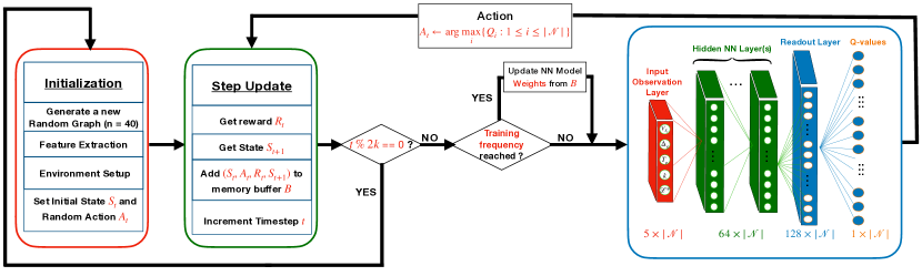
Figure 1: Overview of RELS-DQN training: 1) We generate a random ER graph with fixed size and initialize the environment for each training episode, where $t$ labels the iteration of timesteps; 2) Each element’s parameters (denoted $x_{e}=\{V_{\{e\}},\Delta_{e},\mathcal{T}_{e},V_{k_{e}},\mathcal{L}^{*}\}$, Section IV-A) are updated and passed to the feed-forward network to calculate the Q-value, where the numbers below each layer are input/output vector dimension, and $|\mathcal{N}|$ is the ground set size; 3) Based on the $\epsilon$-greedy action rate of training, the agent’s action $A_{t}$ will either be randomly chosen (exploration) or through a greedy-policy (exploitation, $A_{t}\leftarrow\arg\max_{i}\{Q_{i}\}$); 4) Using action $A_{t}$, get the reward $R_{t}$ and the new state $S_{t+1}$ to update the environment and the network (if training frequency is reached); 5) Every $2k$ timesteps, we generate a new graph and repeat Steps (1) - (4) until the total timesteps $t=$ 1 million.

II Related work

The advancements in AI techniques introduced new heuristic approaches based on deep learning [6, 28, 8, 29, 30, 31, 32]. One of the techniques is GNN, which has gained attention in solving graph-based combinatorial problems by aggregating information from the neighborhood to update node representations. This recursive aggregation scheme based on neighborhood relationships has proven to be a powerful technique in processing the representation of graphs [7, 33, 5, 21, 8, 30, 31, 32]. In general, these GNN-based approaches require either one-hot encoded vectors [7, 32, 8] or node feature matrix [5, 21, 30, 31] as initial embeddings, which can be smoothed by the neighborhood aggregation to carrier graph structure information. However, recent studies have highlighted the inherent over-smoothing and information loss issues of GNNs [23, 24, 25, 26]. This over-smoothing problem can also affect solving combinatorial optimization problems, as the goal is to identify distinguished nodes that maximize the objective function.

Reinforcement Learning combined with GNNs is becoming increasingly popular for solving CO problems. Most notably, [7] proposed S2V-DQN, a GNN-based reinforcement learning approach, which uses the neighborhood aggregation to update the node representation and learns a greedy policy using Q-learning with the graph embedding vector. However, the state of S2V-DQN only considers the adjacency matrix and the state of nodes, and simply follows greedy policy at every step, which results in subpar performance [22]. As data size continuously increases, developing models that can scale to modern dataset sizes is imperative. Significant improvement in scalability can be seen in GComb [21]. GComb uses a probabilistic greedy mechanism to predict the quality of the nodes by a trained GCN. By evaluating the quality of nodes, GComb is able to prune those unlikely to be in the solution set, allowing it to generalize to large graphs of millions or billions of nodes while maintaining the performance of S2V-DQN on Maximum Coverage on the bipartite graph (MCP), Maximum Vertex Cover (MVC), and Influence Maximization (IM). However, similar to S2V-DQN, it does not involve local search behavior resulting in its performance being marginally lower than S2V-DQN.

Therefore, [5] proposes ECO-DQN, an improvement over S2V-DQN by allowing the agent to explore, i.e., the agent allows performing both adding or removing actions, known as reversible action. The removal action allows the agent to step back, re-evaluate the states, and improve solutions better than the greedy. Their demonstration shows that the ECO-DQN outperforms S2V-DQN and MaxCutApprox algorithm [5] (greedy-based) in the MaxCut problem with negative edge weight. The model uses the normalized observations of nodes as messages and the neighborhood normalization for aggregation, which are beneficial for node-specific tasks and for cases where the observation values vary significantly. However, the normalized node features not only lead to information loss after several iterations of message passing but also limited the model to application-specific problems. Although ECO-DQN has demonstrated good performance, it encounters memory scaling challenges when applied to large and dense graphs, particularly when the message has high-dimensional vector space computed by an initial embedding layer.

In addition, more recent works have investigated local search techniques to address the combinatorial optimization problem. For example, [22] proposed an approach based on tree search, which utilizes GCN to present a probability map and then refine the solution with a local search algorithm. This approach requires iterations over all vertices to find a replacement, which is an inevitable step in the local search. In a study by [30], they formulate a scheduling problem with sequential selection as a Markov Decision Process (MDP) and use RL to learn a parameterized policy with local search actions employing the GNN-based encoder. The trained RL can learn the local search by acceptance, neighborhood selection, and perturbations, yielding additional iterations like local search algorithms. Another work related to our approach is [9], which uses reinforcement learning with MPNN to adopt an expensive swapping search in size of $O(n^{2})$. Overall, these works show that even though the results of [7, 5, 22, 9, 30] show a promising prospect of finding better solutions than greedy, the local search and MPNN methods remain challenges in solving combinatorial optimization problems. The proposed model RELS-DQN explores the possibility of the RL agent learning a heuristic exploration strategy without relying on message passing and if it can generalize to various cardinality-constrained combinatorial optimization problems.

III Preliminaries

RL Encoding: The combinatorial optimization problem is defined in the standard RL framework as follows:

• States $S$: is a vector of the environment representation which usually includes graph embeddings [7, 5]. In our model, the state is a sequence of elements on graph $G$, and its embedding representation is a set of element-specific parameters $\{x_{e_{1}},x_{e_{2}},\dots,x_{e_{n}}\}$ (Section IV-A). It is easy to see that this representation of the state can be used across different applications as each parameter is weighted the same by the pre-trained network model.

• Actions $a$: is an element $e$ from $\mathcal{N}$, which adds or removes this element from the solution set by flipping the incumbent state $V_{\{e\}}$ (Section IV-A, the value is flipped to 1 if $e\notin V$ and to 0 if $e\in V$, where $V$ is the partial solution of current state $S$), and updates other parameters in $x_{e}$.

• Rewards $R(S,a)$: is defined as the difference in the objective function after updating the state [7], which is $R(S,a)=f(S^{\prime})-f(S)$, where $S^{\prime}$ is the state after current state $S$ taking action $a$. In this case, the cumulative reward $R$ at the terminal state is the objective function value. In our model, the reward is shaped to incorporate constraint in Section IV-C.

• Transition $(S,a,R,S^{\prime})$: uses tuple to present the process of moving from $S$ to $S^{\prime}$ with giving action $a$.

Double Q-learning: Double Deep Q-network (Double DQN) [34] is an off-policy reinforcement learning algorithm that reduces the overestimation of DQN to improve the accuracy of value estimation. A target network with the same architecture as the original DQN is periodically updated to obtain the Q-value. The Q-value function of the target network is defined as follows:

$$Q^{target}\equiv R(S,a)+\gamma Q(S^{\prime},\underset{a}{\arg\max}\ Q(S^{\prime},a;\theta),\theta^{target}),$$ (1)

where $\theta$ is the online weights updated by $S$, $\theta^{target}$ is the target network weights updated by $S^{\prime}$, and $\gamma\in[0,1)$ is the discount factor.

Algorithm 1 ReversibleLocalSearch$(f,\mathcal{N},k,\lambda_{\Delta},\lambda_{t})$

1:Input: evaluation oracle $f:2^{\mathcal{N}}\to\mathbb{R}$, constraint $k$, marginal gain influence weight $\lambda_{\Delta}$, element age influence weight $\lambda_{t}$

2:Let $V\leftarrow\emptyset$, $V^{*}\leftarrow\emptyset$, $t=0$

3:$f(e|V)=f(V\cup\{e\})-f(V)$ if $e\notin V$, otherwise $f(V$ \$\{e\})-f(V)$

4:$\mathcal{T}\leftarrow\{t_{e}=0$ ; $e\in\mathcal{N}\}$

5:for $t=1$ to $2k$  do

6:     $\mathcal{T}\leftarrow\{t_{e}+1$ ; $e\in\mathcal{N}\}$

7:     $\Delta\leftarrow\{f(e|V)$ : $e\in\mathcal{N}\}$

8:     $x\leftarrow\arg\max_{e}\{\lambda_{\Delta}\cdot\Delta_{e}+\lambda_{t}\cdot\mathcal{T}_{e}$ ; $e\in\mathcal{N}\}$

9:     if $\Delta_{x}>0$ or $|V|\leq k$ then

10:         if $x\notin V$ then

11:              $V\leftarrow V\cup\{x\}$

12:         else

13:              $V\leftarrow V$ \$\{x\}$

14:         end if

15:         $\mathcal{T}_{x}\leftarrow 0$

16:         $V^{*}\leftarrow\arg\max\{f(V^{*}),f(V)\}$

17:     else

18:         $x\leftarrow\arg\max_{e}\{\lambda_{\Delta}\cdot\Delta_{e}+\lambda_{t}\cdot\mathcal{T}_{x}$ ; $e\in V\}$

19:         $V\leftarrow V$ \$\{x\}$

20:     end if

21:end for

22:return $V^{*}$

IV RELS-DQN

To start, we modified the local search algorithm [20] to allow it to explore unvisited nodes after a few iterations instead of extra queries after each selection of the maximum singleton. In Algorithm 1, we provide two parameters to balance the weight of exploration and greedy selection. For each node, we set up an element-wise initialized timer $\mathcal{T}$ (line 4) to track if the node has been visited yet. The $2k$ iterations imply two stages of selection. In the first $k$ iterations, the marginal gain of the objective function $\delta_{e}$ is selected greedily as the $\mathcal{T}_{e}$ remains the same for $e\notin V$. As for the second $k$ iteration, the unvisited nodes have a larger weight on $\mathcal{T}_{e}$ to encourage exploring new nodes instead of following the margin gain. However, it is infeasible to find the best weight parameters that apply to various applications.

Next, we propose RELS-DQN inspired by [5]. Our model mimics the behavior of the general-purpose local search algorithm defined in Algorithm 1, and balances the greedy policy and exploration through a network model instead of weight parameters. RELS-DQN modified the environment observations in [5]. We provide element-wise defined parameters (Section IV-A) as the representation of the environment state. Our model uses a lightweight feed-forward network (Section IV-B) that provides the flexibility to learn an application. This network can apply to different applications while remaining efficient in terms of memory and runtime. As for the reward shaping (Section IV-C), we use the cardinality constraint $k$ as part of reward shaping to enable exploration of the local optimal solution within the constraint limitation. Figure 1 illustrates the training framework of RELS-DQN, where it explores small randomly generated synthetic graphs to learn how to obtain solutions through local search behavior.

IV-A Element Parameters

In this section, a set of parameters are defined at the element level to describe the current state of the environment. These parameters provide the feature representation to the RL model for balancing exploration, exploiting the greedy policy, and taking into account constraint limitation. Existing models such as S2V-DQN [7] and ECO-DQN [5] use one and seven element-specific parameters respectively for solution selection. While these are performant models, their lack of constraint parameters hinders their ability to handle constrained problems. In addition, S2V-DQN only uses one element parameter which restricts its local search capability, while the seven parameters of ECO-DQN lead to redundancy due to its global observations. Therefore, we list the parameters used in our model as follows:

• Incumbent State $V_{\{e\}}$ is a binary bit to indicate if the element is selected or not in current state $S$, such that it is 1 if $e\in V$; otherwise 0. This parameter of the entire set is denoted as $V_{S}$, such that the partial solution $V$ is denoted as $V=\{x\in V_{S}|x=1\}$.

• Marginal Gain $\Delta_{e}$ is the gain/loss of adding/removing element $e\in\mathcal{N}$ from the partial solution $V$. This parameter encourages the model to maximize the gain regardless of whether the action is removing or adding an element.

• Inactive Age $\mathcal{T}_{e}$ provides the timestep that element $e\in\mathcal{N}$ has not been selected as the action $a$. It is reset to 0 every time $a\leftarrow\{e\}$, which discourages the model from selecting the same action every iteration and aid in extensive exploration of the solution space.

• Feasible candidate $V_{k_{e}}$ provides the permissible actions of an element. For the entire set, its candidate state is represented as $V_{k}$. This parameter discourages the model to generate a solution set size larger than $k$ and encourages removing action when it exceeds constraint limitation. For this parameter, all elements are set to 1 if $|V|\leq k$; otherwise, only the elements in the partial solution set are 1, and the rest elements are 0.

• Distance to local optimum $\mathcal{L}^{*}$ is the distance of current $f(S)$ to the best observed $f(S^{*})$. The $S^{*}$ is the state of the best solution that is updated when $f(S)>f(S^{*})$ at the end of each timestep. As the actions reducing solution value are possible, we need this parameter to track the best solution that has been encountered during the episode.

IV-B Network Architecture

The DQN network architecture determines how the Q-value for the action policy is calculated. Existing literature has primarily focused on GCN [35, 36, 21] and MPNN [7, 5] to determine the best action based on the updated node embedding from the neighborhood aggregation. While the GNN aggregates information from local graph neighborhoods and the embeddings are encoded with the multi-hop neighbors, it also smooths the features that are well-designed to intuitively reflect the environment state. Especially, the parameters defined as the environment state in section IV-A are additional information that is not attached to nodes and edges and should avoid any operation that can cause information loss, such as neighborhood normalization [37]. Therefore, these advantages of GNN adversely impact the robustness and ability to solve various combinatorial optimization problems. Additionally, the memory overhead of MPNN and GCN network architecture can limit their scalability to large data instances. RELS-DQN addresses the robustness and scalability concerns of the MPNN-based models by utilizing two fully connected feed-forward layers with ReLu activation functions represented as follows:

$$\mu_{e}=\text{ReLu}(\theta_{2}~{}\text{ReLu}(\theta_{1}x_{e})),$$ (2)

where $x_{e}=\{V_{\{e\}},\Delta_{e},\mathcal{T}_{e},V_{k_{e}},\mathcal{L}^{*}\}\in\mathbb{R}^{5}$ is the feature vector of a single element $e\in\mathcal{N}$, and $\mu$ is its output vector from the hidden layers. $\theta_{1}\in\mathbb{R}^{m\times 5},\theta_{2}\in\mathbb{R}^{m\times m}$ are the weight of the corresponding layers, and $m$ is the number of neurons in the hidden layers.

The feed-forward layers directly capture information about the environment representations and use its weight matrix and ReLu activation function to produce the hidden features. Then, the readout layer produces the Q-value from each element’s hidden feature $\mu_{e}$ and the pooled embedding over the ground set as follows:

$$Q_{e}=\theta_{4}[\text{ReLu}(\theta_{3}\frac{1}{|\mathcal{N}|}\sum_{u\in\mathcal{N}}\mu_{u}),\mu_{e}],$$ (3)

where $\theta_{3}\in\mathbb{R}^{m\times m}$, $\theta_{4}\in\mathbb{R}^{2m}$, $\left[\cdot,\cdot\right]$ is the concatenation operator, and $|\mathcal{N}|$ represents the number of elements in ground set. The embedding of the ground set $\mu_{u},u\in\mathcal{N}$ uses the shared $\mu_{e}$, which is later normalized with $|\mathcal{N}|$ and fed into a linear pooling layer with ReLu activation function. The concatenation of the $\mu_{e}$ and the pooled embedding over the ground set, $\text{ReLu}(\theta_{3}\frac{1}{|\mathcal{N}|}\sum_{u\in\mathcal{N}}\mu_{u})$, is used to extract the Q-value so that the model selects the action $a\leftarrow\arg\max_{i}\{Q_{i}:1\leq i\leq|\mathcal{N}|\}$.

IV-C Reward reshaping

The reward reshaping of RELS-DQN primarily consists of the state reward $F(V_{S})$ and the constraint reward $D(V_{S})$ in order to find the best solution within constraints by exploration. Given the state reward $F(V_{S})=max(f(S)-f(S^{*}),0)$ and the constraint reward $D(V_{S})=k-|V|$, the non-negative reward for solving constrained instances is formally given as follows:

$$R(S,a)=\begin{cases}\hfil max\{\frac{F(V_{S})\times D(V_{S})}{|\mathcal{N}|},0\}&a\notin V,|V|\geq k\\ \hfil max\{\frac{F(V_{S})}{|\mathcal{N}|},0\}&\text{, otherwise}\end{cases}$$ (4)

where $V_{S}$ is the incumbent state at state $S$; $S^{*}$ is the best observed state up to current state and $k$ is the cardinality constraint.

The state reward $F$ provides a positive reward when an action improves the objective value over the best-observed state $S^{*}$ and does not receive a penalty when the action reduces the solution value. On the other hand, the constraint reward $D$ works as follows: if the size of the solution is within the constraint limitation $|V|<k$, the agent receives the state reward; if $|V|\geq k$, the agent is encouraged to remove an element $e$ from the partial solution $V$ by adding a penalty to the adding action. Additionally, the exploration is considered by removing all penalties and not rewarding the agent unless the solution is improved. Therefore, reward shaping considers two scenarios: if the agent takes any actions within the constraint limit or the removing actions at $|V|\geq k$, the environment provides the state reward; if the agent takes the adding action at $|V|\geq k$, the environment changes any positive reward into zero by providing the constraint penalty $D<0$. In this case, the environment only provides a positive reward when a better solution is found within the constraint, and the non-negative reward allows the agent to explore actions that can reduce the solution value.

V Empirical Evaluation

In this section, we analyze the effectiveness and efficiency of RELS-DQN as a general purpose algorithm. We provide the source code link that includes experimental scripts and datasets. With our empirical evaluations, we address the following questions:

Question 1: Is a shallow network architecture better at solving CO problems than deep neural networks?

Question 2: Can the RELS-DQN model solve a diverse set of problems without application-specific training?

Question 3: How efficient is RELS-DQN compared to the MPNN-based ECO-DQN and Greedy-LS?

V-A Experiment setup

Applications: Our experiment set consists of a set of four diverse combinatorial optimization problems: Maximum Cut (MaxCut) [5], Directed Vertex Cover with Costs (MaxCov) [38], Movie Recommendation (MovRec) [13], and Influence-and-Exploit Marketing (InfExp) [39]. Details of all applications and their objective functions are defined as follows:

Maximum Cut Problem (MaxCut) is defined as follows. For a given graph $G(\mathcal{N},E,w)$, where $\mathcal{N}$ represents the set of vertices, $E$ denotes the set of edges, and $w:E\rightarrow\mathbb{R}^{*}$ represents the weight of edges with $w\in\{0,\pm 1\}$. Find a subset of nodes $V\subseteq\mathcal{N}$ such that the objective function is maximized: [5]

$$f(V):=max\sum_{u\in V,v\in\overline{V}}w(u,v),$$ (5)

where $\overline{V}=\mathcal{N}\setminus V$ represents the complementary set. In addition, the constrained MaxCut problem projects to $|V|\leq k$, in which $0<k\leq|\mathcal{N}|$ is a constraint.

Directed Vertex Cover with Costs (MaxCov) is defined as follows. For a given directed graph $G(\mathcal{N},E,w)$, let $w:E\rightarrow\mathbb{R}$. For a subset of nodes $V\subseteq\mathcal{N}$, the weighted directed vertex cover function is $g(V)=\sum_{u\in N(V)\cup V}w_{u}$, where $N(V)$ represents the set of nodes pointed by the subset $V$. [38] assumes that there is a nonnegative cost $c_{n}$ for each $n\in\mathcal{N}$. Therefore, the objective function is defined as [38]:

$$g(V)-c(V):=\sum_{u\in N(V)\cup V}w_{u}-\sum_{u\in V}c_{u},$$ (6)

where the cost associated with each node is set to $c(n)=1+max\{d(n)-q,0\}$ for a fixed cost factor $q=6$ and the out-degree $d(n)$ of $n\in\mathcal{N}$.

Movie Recommendation (MovRec) produces a subset from a list of movies for a user based on other users with similar ratings. We use the objective function in [13] defined as follows:

$$f(V):=\sum_{i\in\mathcal{N}}\sum_{j\in V}s(i,j)-\lambda\sum_{i\in V}\sum_{j\in V}s(i,j)$$ (7)

Where $s_{ij}$ is the inner product of the ratings vector between movie $i$ and $j$, and $\lambda=5$ is the diversity coefficient which the large $\lambda$ penalizes similarity more [39].

Influence-and-Exploit Marketing (InfExp) consider how the buyers of a social network can influence others to buy goods for revenue maximization. For a given set of buyer $\mathcal{N}$, each buyer $i\in\mathcal{N}$ is associated with a non-negative concave function $f_{i}(x)=a_{i}\sqrt{x}$ where the $a_{i}$ a number followed by Pareto Type II distribution with $\lambda=1,\alpha=2$ [39]. For a given subset $V\subseteq\mathcal{N}\setminus\{i\}$ of buyer $i$, the objective function is defined as follows [39]:

$$f(V):=\sum_{i\in\mathcal{N}\setminus V}f_{i}(\sum_{j\in V\cup\{i\}}w_{ij})$$ (8)

where the weight of the graph is uniformly randomly generated from $U(0,1)$.

TABLE II: Dataset and graph size.

Application	Dataset	$|\mathcal{N}|$	$|E|$
MaxCut	ego-Facebook(fb4k)	4039	88234
MaxCut	musae-FB(fb22k)	22470	171002
MaxCov	email-Eu-core(eu1k)	1005	25571
MovRec	MovieLens(mov1.7k)	1682	983206
InfExp	BarabásiAlbert(ba300)	300	1184

Benchmarks: We compare RELS-DQN to the MPNN heuristic framework ECO-DQN [5], the standard greedy algorithm (Greedy), the vanilla local search algorithm (Greedy-Rev) and the local search algorithm[10] (Greedy-LS). The ECO-DQN serves as a benchmark after adapting the feasible candidate $V_{k}$ in environment observation and the constrained reward function. Greedy-Rev is a greedy algorithm that allows reversible actions to arrive at a better value until no further improvement is possible. Greedy-LS meanwhile repeats itself within the cardinality constraint $k$, checking if the existing nodes satisfy the credentials for removing or swapping after every new addition. Additionally, we use sparse representation on MPNN using Torch-Geometric to evaluate memory improvement.

Training: RELS-DQN model is trained on MaxCut only, and ECO-DQN models are trained on specific applications. ECO-DQN model is modified and adapted to the constrained problem by applying feasible candidate parameter $V_{k}$ (Section IV-A) and reward shaping(Section IV-C). We train all models using synthetic graphs ($n$=40, $k$=30) with each episode $2k$ timesteps to make sure each graph is explored entirely and the element parameters are learned sufficiently. The synthetic training data is generated in the following ways:

• MaxCut: Erdös-Rényi graphs (ER) [40] with probability $p=0.15$ and edge weight $w_{ij}\in\{0,\pm 1\}$.

• MaxCov: ER graphs with $p=0.15$ and $w_{ij}\in\{0,+1\}$.

• MovRec: ER graphs with $p=0.15$ and $w_{ij}\in(0,1)$ generated uniformly randomly.

• InfExp: Barabasi-Albert graph (BA) [41] with $m=4$ and $w_{ij}\in(0,1)$ generated uniformly randomly.

Testing: RELS-DQN model uses the pre-trained model of MaxCut to validate all applications and datasets. Conversely, the ECO-DQN model uses the application-specific pre-trained model for each problem. We evaluate the performance using synthetic ER graph ($n$=200, $p$=0.03), BA graph ($n$=200, $m$=4) and large datasets listed in Table II. In addition, all applications are validated on a hundred graphs except the InfExp is validated on ten graphs.

Hardware environment: We run all experiments on a server with a TITAN RTX GPU (24GB memory) and 80 CPU Intel(R) Xeon(R) Gold 5218R cores.

V-B Architecture Evaluation

In this section, we describe the learning characteristics of the DQN models on the MaxCut problem. Figure 2a compares the training performance of RELS-DQN by increasing the number of hidden layers in Equation 2 up to 8 layers. As shown, RELS-DQN-2 and RELS-DQN-4 converge to the highest solution value, and RELS-DQN-2 exhibits the ability to converge earlier. RELS-DQN-6 cannot converge to a high value, while RELS-DQN-8 shows the inability to learn the MaxCut problem. These results demonstrate the adverse effect of using a complex neural network architecture to solve combinatorial problems. Based on our evaluation, we choose RELS-DQN-2 as our model for all evaluations as it demonstrates the best learning ability. In figure 2b, we observe that both RELS-DQN-2 and ECO-DQN converge to the best solution with ours converging earlier. S2V-DQN cannot achieve higher solution values due to its lack of local search.

Figure 2: The learning curves of the RL models for MaxCut on ER-40 graph. RELS-DQN and ECO-DQN converge to a higher solution value than S2V-DQN while RELS-DQN reaches convergence earlier than ECO-DQN.

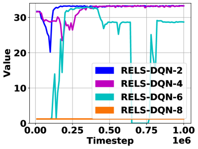
(a)

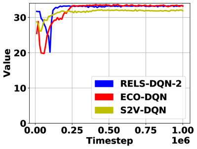
(b)

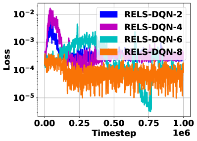
(c)

(d)

Figure 3: Ilustrates the testing results of RELS-DQN, ECO-DQN, Greedy, Greedy-Rev and Greedy-LS on four applications. RELS-DQN uses the pre-trained model of MaxCut (ER, $n=$40) for all applications, while ECO-DQN uses application-specific model for each application. The $timeout$ for each application is set to 24 hours.

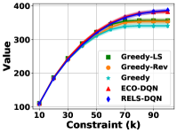
(a) MaxCut (ER200)

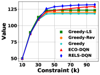
(b) MaxCov (ER200)

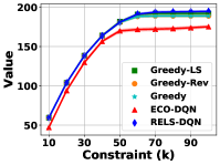
(c) MovRec (ER200)

(d) InfExp (BA200)

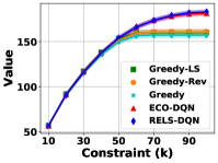
(e) MaxCut (BA200)

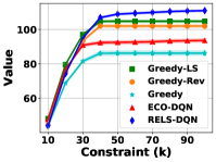
(f) MaxCov (BA200)

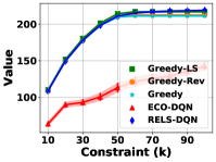
(g) MovRec (BA200)

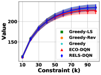
(h) InfExp (ER200)

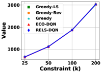
(i) MaxCut (fb4k)

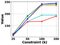
(j) MaxCov (eu1k)

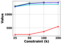
(k) MovRec (movielen1.7k)

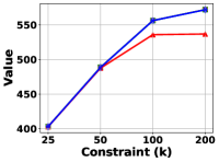
(l) InfExp (ba300)

Figure 4: The runtime results of RELS-DQN, ECO-DQN and the best local search baseline Greedy-LS on the large datasets (see Table II) of four applications. The $timeout$ for each application ($k=\{25,50,100,200\}$) is set to 24 hours.

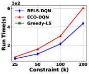
(a) MaxCut (fb4k)

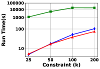
(b) MaxCov (eu1k)

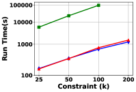
(c) MovRec (movielen1.7k)

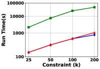
(d) InfExp (ba300)

V-C Generalization Evaluation

In this section, we test the ability of RELS-DQN to provide feasible solutions to various combinatorial problems without application-specific training. To evaluate its generalization, we compare the MaxCut trained RELS-DQN (ER graph, $n=$40) to the application-specific trained ECO-DQN (ER graph, $n=40$), Greedy, and Greedy-LS and Greedy-Rev across four applications. We evaluate the models on synthetic and real-world datasets for each application. As part of the synthetic dataset experiments (Figure 3a-3h), all models are run on a hundred randomly generated synthetic graphs, with the mean solution value plotted.

RELS-DQN Vs. Greedy The empirical comparison of RELS-DQN to the Greedy, the Greedy-Rev, and the Greedy-LS demonstrates our model’s ability to provide solutions with values higher than or equal to these general-purpose greedy-based algorithms. As illustrated in Figure 3l, due to its lack of local-search capability, Greedy is surpassed by Greedy-Rev and Greedy-LS in terms of solution value, with Greedy-LS consistently providing similar or outperforming Greedy-Rev across all applications. For the MaxCut and MaxCov problem on the ER datasets (Figure 3a, 3b), RELS-DQN outperforms Greedy-LS by 2% and 3% respectively on average, with indiscernible results for the other applications. Additionally, RELS-DQN provides 5% and 1.5% improvement in solution value over Greedy-LS for MaxCut and MaxCov on BA datasets, with near-identical results on other applications and large datasets. RELS-DQN’s improvement over Greedy-LS can be attributed to its enforced exploration (Alg. 1, Line 18 - 19), which allows the model to search for better solutions even when local-search criteria (Alg. 1, Line 9 - 16) indicate no possibility of adding or removing elements. Across all instances, RELS-DQN outperforms Greedy, Greedy-Rev, and Greedy-LS by 5%, 2%, and 1%, respectively. It is evident from the comparison that RELS-DQN’s local-search capability can provide feasible solutions in various applications without requiring application-specific training, proving its utility as a general-purpose algorithm. Individual application results are provided in Table I.

RELS-DQN Vs. ECO-DQN Across all datasets, ECO-DQN and RELS-DQN provide near-identical solution values for the MaxCut problem. As shown in Figure 3b-3d, for MaxCov, MovRec, and InfExp on ER graphs, RELS-DQN consistently outperforms ECO-DQN with a 5% average improvement in solution value across these instances. Extending the experiment set to the BA datasets (Figure 3f - 3h), we observe that RELS-DQN provides an average improvement of 28% across the MaxCov, MovRec and InfExp application, with this improvement increasing to 114% for real-world datasets (Figure 3j - 3l). In addition, Table I indicates that the difference between ECO-DQN and RELS-DQN is minimal for ER datasets as the models are trained on ER graphs for each application, and the performance gap increases with changes in graph type and size. The comparison validates the generalization consistency of RELS-DQN to maintain or outperform application-specific ECO-DQN models’ performance across a wide range of combinatorial applications and datasets.

V-D Efficiency Evaluation

Runtime Evaluation: We compare the runtime performance of RELS-DQN to ECO-DQN and the best local-search baseline Greedy-LS for the real-world datasets. Figure 4b - 4d illustrates that RELS-DQN provides a 264, 64, and 36 times speedup over Greedy-LS for MaxCov, MovRec and InfExp respectively. Additionally, for the MaxCut problem, Greedy-LS does not complete a single constraint instance within the 24 hours timeout. As shown in Figure 4a, 4c and 4d, RELS-DQN is 40%, 7% and 8% faster than ECO-DQN for the MaxCut, MovRec and InfExp problem. Across all applications, RELS-DQN provides a 10% runtime improvement over ECO-DQN on average. The results exemplify RELS-DQN’s ability to maintain or outperform the Greedy-LS in terms of solution value while providing an order-of-magnitude speedup in completion time.

Memory evaluation: We observe the GPU memory usage using the $pynvml$ package. For ECO-DQN, we monitor two variants, ECO-DQN, which uses an adjacency matrix for its graph representation, and ECO-DQN-sparse, a sparse matrix implementation for MPNN. Table III presents the memory usage of these models with “-” representing scenarios when an out-of-memory crash occurred. Evaluations are performed on two real-world datasets, fb4k ($n=$4,039 ) and fb22k ($n=$22,470) with batch sizes 1 (Postfix “-batch1”) and 5. ECO-DQN with dense representation (adjacency matrix) runs out of GPU memory on 3 out of 4 instances, with the only instance it completes being fb4k for batch size = 1. While ECO-DQN-sparse drastically improves the memory overhead of ECO-DQN, RELS-DQN on average across all scenarios provides a 30% improvement over ECO-DQN-sparse.

TABLE III: GPU usage (MB).

Network type	fb4k-batch1	fb4k	fb22k-batch1	fb22k
RELS-DQN	1459	1725	3335	11197
ECO-DQN	10483	-	-	-
ECO-DQN-sparse	1571	2489	5249	20663

VI Conclusion

In this paper, we have introduced RELS-DQN, a novel DQN model that demonstrates the ability to perform the local search across a diverse set of combinatorial problems without application-specific training. Unlike existing models, utilizing a compressed feature space and a simpler network architecture allows our model to behave like a general-purpose algorithm for combinatorial problems. Our claims are exemplified through an extensive evaluation of a diverse set of applications that illustrates RELS-DQN’s ability to provide feasible solutions on all four instances of constrained CO problems, with significant speedup over ECO-DQN and Greedy-LS. In addition, the reduction in memory footprint compared to MPNN models encourage RELS-DQN’s scalability to real-world combinatorial problems. The combined improvement in both generalization and efficiency suggests that the environment states contain valuable information that should not be used as messages in GNN. The future study direction should consider feature-based and structural information separately and analyze their individual effects before exploring their combined impact. On the other hand, our framework also has several limitations. The CO problems that require the ordered sequence are not feasible, such as TSP, because our framework focuses on selecting a subset in an arbitrary order that maximizes the objective function. Another limitation is that the environment representation is element-wise parameters and requires margin gain calculation, which is computationally expensive and the efficiency can be further improved by reducing the number of query times in margin gain calculation.

References

- [1] Michel X Goemans and David P Williamson. Improved approximation algorithms for maximum cut and satisfiability problems using semidefinite programming. Journal of the ACM (JACM), 42(6):1115–1145, 1995.
- [2] Irit Dinur and Samuel Safra. On the hardness of approximating minimum vertex cover. Annals of mathematics, pages 439–485, 2005.
- [3] Karla L Hoffman, Manfred Padberg, Giovanni Rinaldi, et al. Traveling salesman problem. Encyclopedia of operations research and management science, 1:1573–1578, 2013.
- [4] Kenshin Abe, Zijian Xu, Issei Sato, and Masashi Sugiyama. Solving np-hard problems on graphs with extended alphago zero. arXiv preprint arXiv:1905.11623, 2019.
- [5] Thomas Barrett, William Clements, Jakob Foerster, and Alex Lvovsky. Exploratory combinatorial optimization with reinforcement learning. In Proceedings of the AAAI Conference on Artificial Intelligence, volume 34, pages 3243–3250, 2020.
- [6] Irwan Bello, Hieu Pham, Quoc V Le, Mohammad Norouzi, and Samy Bengio. Neural combinatorial optimization with reinforcement learning. arXiv preprint arXiv:1611.09940, 2016.
- [7] Hanjun Dai, Elias B Khalil, Yuyu Zhang, Bistra Dilkina, and Le Song. Learning combinatorial optimization algorithms over graphs. arXiv preprint arXiv:1704.01665, 2017.
- [8] Quentin Cappart, Thierry Moisan, Louis-Martin Rousseau, Isabeau Prémont-Schwarz, and Andre Cire. Combining reinforcement learning and constraint programming for combinatorial optimization. arXiv preprint arXiv:2006.01610, 2020.
- [9] Fan Yao, Renqin Cai, and Hongning Wang. Reversible action design for combinatorial optimization with reinforcement learning. arXiv preprint arXiv:2102.07210, 2021.
- [10] Jon Lee, Vahab S Mirrokni, Viswanath Nagarajan, and Maxim Sviridenko. Non-monotone submodular maximization under matroid and knapsack constraints. In Proceedings of the forty-first annual ACM symposium on Theory of computing, pages 323–332, 2009.
- [11] Anupam Gupta, Aaron Roth, Grant Schoenebeck, and Kunal Talwar. Constrained non-monotone submodular maximization: Offline and secretary algorithms. In International Workshop on Internet and Network Economics, pages 246–257. Springer, 2010.
- [12] Baharan Mirzasoleiman, Stefanie Jegelka, and Andreas Krause. Streaming non-monotone submodular maximization: Personalized video summarization on the fly. In Proceedings of the AAAI Conference on Artificial Intelligence, volume 32, 2018.
- [13] Matthew Fahrbach, Vahab Mirrokni, and Morteza Zadimoghaddam. Non-monotone submodular maximization with nearly optimal adaptivity and query complexity. In International Conference on Machine Learning, pages 1833–1842. PMLR, 2019.
- [14] Alan Kuhnle. Nearly linear-time, parallelizable algorithms for non-monotone submodular maximization. In Proceedings of the 35th AAAI conference on artificial intelligence, 2021.
- [15] Yixin Chen, Tonmoy Dey, and Alan Kuhnle. Best of both worlds: Practical and theoretically optimal submodular maximization in parallel. Advances in Neural Information Processing Systems, 34, 2021.
- [16] Tonmoy Dey, Yixin Chen, and Alan Kuhnle. Dash: Distributed adaptive sequencing heuristic for submodular maximization. arXiv preprint arXiv:2206.09563, 2022.
- [17] Anna Galluccio, Martin Loebl, and Jan Vondrák. Optimization via enumeration: a new algorithm for the max cut problem. Mathematical Programming, 90(2):273–290, 2001.
- [18] Alexander A Lazarev, Ivan Nekrasov, and Nikolay Pravdivets. Evaluating typical algorithms of combinatorial optimization to solve continuous-time based scheduling problem. Algorithms, 11(4):50, 2018.
- [19] George L Nemhauser, Laurence A Wolsey, and Marshall L Fisher. An analysis of approximations for maximizing submodular set functions—i. Mathematical programming, 14(1):265–294, 1978.
- [20] Andrew An Bian, Joachim M Buhmann, Andreas Krause, and Sebastian Tschiatschek. Guarantees for greedy maximization of non-submodular functions with applications. In International conference on machine learning, pages 498–507. PMLR, 2017.
- [21] Sahil Manchanda, Akash Mittal, Anuj Dhawan, Sourav Medya, Sayan Ranu, and Ambuj Singh. Gcomb: Learning budget-constrained combinatorial algorithms over billion-sized graphs. Advances in Neural Information Processing Systems, 33:20000–20011, 2020.
- [22] Zhuwen Li, Qifeng Chen, and Vladlen Koltun. Combinatorial optimization with graph convolutional networks and guided tree search. Advances in neural information processing systems, 31, 2018.
- [23] Qimai Li, Zhichao Han, and Xiao-Ming Wu. Deeper insights into graph convolutional networks for semi-supervised learning. In Thirty-Second AAAI conference on artificial intelligence, 2018.
- [24] Keyulu Xu, Chengtao Li, Yonglong Tian, Tomohiro Sonobe, Ken-ichi Kawarabayashi, and Stefanie Jegelka. Representation learning on graphs with jumping knowledge networks. In International conference on machine learning, pages 5453–5462. PMLR, 2018.
- [25] Jie Zhou, Ganqu Cui, Shengding Hu, Zhengyan Zhang, Cheng Yang, Zhiyuan Liu, Lifeng Wang, Changcheng Li, and Maosong Sun. Graph neural networks: A review of methods and applications. AI Open, 1:57–81, 2020.
- [26] Tianlong Chen, Kaixiong Zhou, Keyu Duan, Wenqing Zheng, Peihao Wang, Xia Hu, and Zhangyang Wang. Bag of tricks for training deeper graph neural networks: A comprehensive benchmark study. IEEE Transactions on Pattern Analysis and Machine Intelligence, 2022.
- [27] Liang Yang, Junhua Gu, Chuan Wang, Xiaochun Cao, Lu Zhai, Di Jin, and Yuanfang Guo. Toward unsupervised graph neural network: Interactive clustering and embedding via optimal transport. In 2020 IEEE international conference on data mining (ICDM), pages 1358–1363. IEEE, 2020.
- [28] Ruben Solozabal, Josu Ceberio, and Martin Takáč. Constrained combinatorial optimization with reinforcement learning. arXiv preprint arXiv:2006.11984, 2020.
- [29] Nina Mazyavkina, Sergey Sviridov, Sergei Ivanov, and Evgeny Burnaev. Reinforcement learning for combinatorial optimization: A survey. Computers & Operations Research, page 105400, 2021.
- [30] Jonas K Falkner, Daniela Thyssens, Ahmad Bdeir, and Lars Schmidt-Thieme. Learning to control local search for combinatorial optimization. arXiv preprint arXiv:2206.13181, 2022.
- [31] Wouter Kool, Herke van Hoof, Joaquim Gromicho, and Max Welling. Deep policy dynamic programming for vehicle routing problems. In International Conference on Integration of Constraint Programming, Artificial Intelligence, and Operations Research, pages 190–213. Springer, 2022.
- [32] Yeong-Dae Kwon, Jinho Choo, Iljoo Yoon, Minah Park, Duwon Park, and Youngjune Gwon. Matrix encoding networks for neural combinatorial optimization. Advances in Neural Information Processing Systems, 34:5138–5149, 2021.
- [33] Keyulu Xu, Weihua Hu, Jure Leskovec, and Stefanie Jegelka. How powerful are graph neural networks? arXiv preprint arXiv:1810.00826, 2018.
- [34] Hado Van Hasselt, Arthur Guez, and David Silver. Deep reinforcement learning with double q-learning. In Proceedings of the AAAI conference on artificial intelligence, volume 30, 2016.
- [35] Thomas N Kipf and Max Welling. Semi-supervised classification with graph convolutional networks. arXiv preprint arXiv:1609.02907, 2016.
- [36] Natalia Vesselinova, Rebecca Steinert, Daniel F Perez-Ramirez, and Magnus Boman. Learning combinatorial optimization on graphs: A survey with applications to networking. IEEE Access, 8:120388–120416, 2020.
- [37] William L Hamilton. Graph representation learning. Synthesis Lectures on Artifical Intelligence and Machine Learning, 14(3):1–159, 2020.
- [38] Chris Harshaw, Moran Feldman, Justin Ward, and Amin Karbasi. Submodular maximization beyond non-negativity: Guarantees, fast algorithms, and applications. In International Conference on Machine Learning, pages 2634–2643. PMLR, 2019.
- [39] Georgios Amanatidis, Federico Fusco, Philip Lazos, Stefano Leonardi, and Rebecca Reiffenhäuser. Fast adaptive non-monotone submodular maximization subject to a knapsack constraint. arXiv preprint arXiv:2007.05014, 2020.
- [40] Paul Erdos, Alfréd Rényi, et al. On the evolution of random graphs. Publ. Math. Inst. Hung. Acad. Sci, 5(1):17–60, 1960.
- [41] Réka Albert and Albert-László Barabási. Statistical mechanics of complex networks. Reviews of modern physics, 74(1):47, 2002.