An information-theoretic evolutionary algorithm

Abstract

We propose a novel evolutionary algorithm on bit vectors which derives from the principles of information theory. The information-theoretic evolutionary algorithm (it-EA) iteratively updates a search distribution with two parameters, the center, that is the bit vector at which standard bit mutation is applied, and the mutation rate. The mutation rate is updated by means of information-geometric optimization and the center is updated by means of a maximum likelihood principle. Standard elitist and non elitist updates of the center are also considered. Experiments illustrate the dynamics of the mutation rate and the influence of hyperparameters. In an empirical runtime analysis, on OneMax and LeadingOnes, the elitist and non elitist it-EAs obtain promising results.

Keywords: Standard bit mutation, adaptive mutation rate, information geometric optimization, cross-entropy method

1 Introduction

Information theory has revealed itself as a conceptual framework of choice in the field of evolutionary computation, both in the analysis of existing evolutionary algorithms and in the production of new ones . This is especially true of estimation of distribution algorithms [20, 15] which sample an offspring population from a search distribution and estimate its parameters using selected individuals. In particular, algorithms such as MIMIC [6] and UMDA [23] completely rebuild a model at each iteration. They can be expressed in terms of information geometry with a family of probability distributions and a distance between distributions [28, 21]. Standard evolutionary operators, such as mutation and cross-over, can also be interpreted in this framework.

Information geometry is also a valuable resource for the analysis of evolutionary algorithms such as PBIL [4] and CMA-ES [13, 14] which estimate an incremental change in the model parameters as opposed to a full estimate. Starting from PBIL and CMA-ES, a strand of research has lead to the formalization of this approach [5, 30, 22, 29, 24]. In natural evolution strategies (NES) [30, 29] and information-geometric optimization (IGO) [24], incremental changes are determined by means of estimated natural gradients [2] with respect to model parameters. The natural gradient is the gradient in the Fisher metric of the search distribution which, in turn, is expressed in terms of the Kullback–Leibler divergence [19]. The key advantage of natural gradients over Euclidean ones is that the evolution of the search distribution does not depend on the choice of its parameters.

Throughout this paper, we will only be concerned with the search space of fixed-length bit vectors. It is surprising that an evolutionary algorithm on bit vectors similar to CMA-ES is missing. One may object to this observation that PBIL is a natural candidate. However, its parameters are all continuous and, in the form of a probability vector, do not belong to the search space in the same way as, in CMA-ES, the mean of the search distribution does. Furthermore, it is expected that such a speculative evolutionary algorithm will be able to control the mutation rate, just as CMA-ES provides an optimal control of correlated mutations.

Adaptive parameter control in evolutionary algorithms has been the subject of sustained efforts for decades [18, 1]. It has been shown, both in practice and in theory [9], to provide an advantage over fixed parameter strategies. However, update rules are often introduced as heuristics and do not derive from first principles.

A famous update rule is the so called one-fifth success rule [25] which adjusts the mutation rate so as to keep the success rate of mutations equal or close to one fifth (a mutation is successful if it produces an offspring of increased fitness). If the success rate is larger (smaller) than one fifth then the mutation rate should be increased (decreased). The one-fifth constant can be derived from theoretical considerations about the $(1+1)$ evolution strategy applied to the sphere problem in Euclidean spaces. It has been proved that the $(1+1)$ evolutionary algorithm equipped with a similar success-based update rule achieves the same performance on LeadingOnes as the $(1+1)$ EA with an optimal fitness-dependent mutation rate [10]. The 2-rate $(1+\lambda)$ EA with success-based mutation rates achieves the best performance on OneMax among all $\lambda$-parallel black-box algorithms [12].

In another line of research, the problems of operator selection and parameter control have been addressed by means of machine learning, including adaptive pursuit [27] and dynamic multi-armed bandits [7], or reinforcement learning [17]. These methods often assume a finite set of operators or values, hence require the discretization of continuous parameters such as the mutation rate. It is also possible to reason about the number of mutated bits [11] instead of the mutation rate itself. Finally, self-adaptation has been applied to control the mutation rate in genetic algorithms as in evolution strategies [3].

In this work, we propose a novel evolutionary algorithm on bit vectors which derives from the principles of information theory. The information-theoretic evolutionary algorithm (it-EA) iteratively updates a search distribution with two parameters, the center, that is the bit vector at which standard bit mutation is applied, and the mutation rate. The mutation rate is updated by means of information-geometric optimization [24] and the center is updated by means of a maximum likelihood (ML) principle, similar to the cross-entropy method (CEM) [26, 8]. Standard elitist and non elitist updates of the center are also considered.

The paper is organized as follows. The mutation model is presented in Sect. 2. The selection model is presented in Sect. 3. In Sect. 4 and 5, building upon the IGO framework, we derive a precise update rule for the mutation rate. In Sect. 6, we apply a maximum likelihood principle to derive an update rule for the center of the search distribution. The information-theoretic evolutionary algorithm which embeds all the previous principles is presented in Sect. 7. Sect. 8 provides experiments with the it-EA. Sect. 9 concludes the paper.

2 Mutation model

We recall the model of standard mutation of bit vectors and introduce notations as needed. We consider the set $\{0,1\}^{n}$ of $n$-dimensional bit vectors, where $n\in\mathbb{N}^{*}$. The model of standard bit mutation is given by a random bit vector $U$ with independent and identically distributed components. More precisely, for all $u\in\{0,1\}^{n}$,

$$\operatorname{\mathbb{P}}(U=u)=\prod_{i}\operatorname{\mathbb{P}}(U_{i}=u_{i})\,,$$

where $U=(U_{i})$, $u=(u_{i})$, and $i\in[1..n]$. Let $p\in(0,1)$ be the mutation rate. Then,

$$\operatorname{\mathbb{P}}(U_{i}=u_{i})=\begin{cases}p&\text{if $u_{i}=1$}\\ 1-p&\text{if $u_{i}=0$}\end{cases}$$

and

$$\operatorname{\mathbb{P}}(U=u)=p^{\left\|u\right\|}(1-p)^{n-\left\|u\right\|}\,,$$

where $\left\|u\right\|=\sum_{i}u_{i}$ is the Hamming weight (bit count) of $u$. We will denote by $Q_{p}$ the probability distribution of $U$, that is $Q_{p}(u)=\operatorname{\mathbb{P}}(U=u)$.

Let $x$ be some fixed bit vector and suppose that we want to explore the neighborhood of $x$. We define the random vector $V=x\oplus U$, where $U$ has the probability distribution $Q_{p}$ ($U\sim Q_{p}$ for short) and $\oplus$ denotes addition modulo 2. This is similar to the Gaussian case, where $U$ would be a centered Gaussian random vector and $x$ the mean of $V$. However, in the case of bit vectors and addition modulo 2, we cannot speak of mean. Instead, we will say that $x$ is the center of the search distribution.

It turns out that the set $\{Q_{p}:p\in(0,1)\}$ defines an exponential family of probability distributions [22, 24]. Indeed, for all $u\in\{0,1\}^{n}$, $Q_{p}(u)=P_{\theta}(u)$ with

$$P_{\theta}(u)=\frac{1}{Z(\theta)}e^{\theta T(u)}\,,$$ (1)

where $\theta=\operatorname*{logit}(p)$,

$$\operatorname*{logit}(p)=\log\left(\frac{p}{1-p}\right)\,,$$

$T(u)=\left\|u\right\|$, and $Z(\theta)=(1+e^{\theta})^{n}$ is a normalizing constant. The reasons to choose $P_{\theta}$ over $Q_{p}$ are that the IGO flow has a simple expression with exponential families and the evolution of the search distribution is invariant under reparametrization.

3 Selection model

In a black-box context, we want to maximize an arbitrary function $f:\{0,1\}^{n}\rightarrow\mathbb{R}$ defined on bit vectors of dimension $n\in\mathbb{N}^{*}$. Let $x\in\{0,1\}^{n}$ be some fixed bit vector. Let us define $g$, the translated version of $f$, by $g(u)=f(x\oplus u)$, for all $u\in\{0,1\}^{n}$. As in the previous section, $u$ models mutated bits. Following the IGO framework [24], we replace $g$ with a selection weight $W_{\theta}^{g}$. Roughly speaking, for a given $u\in\{0,1\}^{n}$, the smaller the probability of improvement over $u$, the larger its selection weight $W_{\theta}^{g}(u)$.

Assuming maximization of $f$ hence $g$, we define two probabilities of improvement under the sampling distribution $P_{\theta}$. More precisely, for all $u\in\{0,1\}^{n}$,

$$q^{>}(u) =\operatorname{\mathbb{P}}(g(V)>g(u))$$ (2)

$$q^{\geq}(u) =\operatorname{\mathbb{P}}(g(V)\geq g(u))\,,$$

where $V\sim P_{\theta}$. The distinction between comparison operators is necessary since the support of $P_{\theta}$ is $\{0,1\}^{n}$, which implies that

$$\operatorname{\mathbb{P}}(g(V)=g(u))=q^{\geq}(u)-q^{>}(u)$$

is positive for all $u\in\{0,1\}^{n}$. Without this distinction, we could define the selection weight, for all $u\in\{0,1\}^{n}$, by $W_{\theta}^{g}(u)=w(q(u))$, where $w:[0,1]\rightarrow\mathbb{R}$ is a non-increasing function. Instead, it is defined as the mean value of $w$ on the interval $[q^{>}(u),q^{\geq}(u)]$ or

$$W_{\theta}^{g}(u)=\frac{1}{q^{\geq}(u)-q^{>}(u)}\int_{q^{>}(u)}^{q^{\geq}(u)}w(q)\,dq\,.$$ (3)

An important property of the selection weight is that, for all $\theta\in\mathbb{R}$,

$$\operatorname{\mathbb{E}}_{u\sim P_{\theta}}(W_{\theta}^{g}(u))=\int_{0}^{1}w(q)\,dq\,,$$

which only depends on $w$. We will choose $w$ so as to make this expectation equal to 1.

In CMA-ES, at each iteration, $\lambda$ individuals are sampled from $P_{\theta}$ and the $\mu<\lambda$ best ones, according to the fitness function, are used to update the parameter $\theta$. This behavior can be modelled in IGO with the step function $w$ defined, for all $q\in[0,1]$, by

$$w(q)=\frac{1}{q_{0}}1_{q\leq q_{0}}\,,$$ (4)

where $q_{0}=\mu/\lambda$.

4 IGO flow

In the IGO framework, we replace the function to maximize by the expectation of the selection weight with respect to the search distribution. More precisely, let us define the 2-variable function

$$\varphi(\theta,\theta^{\prime})=\operatorname{\mathbb{E}}_{u\sim P_{\theta}}(W_{\theta^{\prime}}^{g}(u))\,.$$

Then, the IGO flow acting on $\theta$ is defined by

$$\frac{d\theta_{t}}{dt}=\tilde{\nabla}_{\theta}\varphi(\theta,\theta_{t})\,,$$

where the natural gradient, denoted by $\tilde{\nabla}$, is taken at $\theta=\theta_{t}$. The natural gradient, as opposed to the Euclidean gradient, is necessary to ensure that the resulting flow does not depend on the particular parametrization that we have chosen for the probability distribution $P_{\theta}$. Although $\theta$ is a scalar, we will stick with the gradient nomenclature. We can express the gradient of the expectation as the expectation of another gradient (log-derivative trick) and write

$$\frac{d\theta_{t}}{dt}=\operatorname{\mathbb{E}}_{u\sim P_{\theta_{t}}}\left(W_{\theta_{t}}^{g}(u)\cdot\tilde{\nabla}_{\theta}\log P_{\theta}(u)\right)\,,$$

where, again, the natural gradient is taken at $\theta=\theta_{t}$. Instead of explicitly computing the natural gradient, we take advantage of the fact that the mutation model defines an exponential family of probability distributions, as we have seen in Sect. 2. The expression of the log-derivative can be found in [22, 24]. The IGO flow can then be expressed as

$$\frac{d\overline{T}}{dt}=\operatorname{\mathbb{E}}_{u\sim P_{\theta_{t}}}\left(W_{\theta_{t}}^{g}(u)\cdot(T(u)-\overline{T})\right)\,,$$

where $\overline{T}=\operatorname{\mathbb{E}}_{u\sim P_{\theta_{t}}}(T(u))$. Since $T(u)=\left\|u\right\|$ and $u\sim P_{\theta_{t}}$, we have $\left\|u\right\|\sim\mathcal{B}(n,p_{t})$ (binomial distribution) and $\overline{T}=np_{t}$. Dividing by $n$ and recalling that $\operatorname{\mathbb{E}}_{u\sim P_{\theta_{t}}}(W_{\theta_{t}}^{g}(u))=1$, we obtain

$$\frac{dp_{t}}{dt} =\operatorname{\mathbb{E}}_{u\sim P_{\theta_{t}}}\left(W_{\theta_{t}}^{g}(u)\cdot\left(\frac{\left\|u\right\|}{n}-p_{t}\right)\right)$$

$$=\operatorname{\mathbb{E}}_{u\sim P_{\theta_{t}}}\left(W_{\theta_{t}}^{g}(u)\cdot\frac{\left\|u\right\|}{n}\right)-p_{t}\,.$$ (5)

The flow can now be interpreted as follows. If the frequency of mutated bits in selected individuals is greater (resp. lower) than the current mutation rate then increase (resp. decrease) it. This is similar to the behavior of the IGO flow acting on the parameters of a Gaussian distribution, in particular its standard deviation. An asymptotic value $p$ for the dynamical system (5) must verify

$$p=\operatorname{\mathbb{E}}_{u\sim P_{\theta}}\left(W_{\theta}^{g}(u)\cdot\frac{\left\|u\right\|}{n}\right)\,,$$ (6)

which means that $p$ must be equal to the frequency of mutated bits in selected individuals. There can be several such fixed-points even if $p_{t}$ can only converge to a unique asymptotic value given an initial condition $p_{0}$.

5 IGO update

Our aim is to provide an evolutionary algorithm with adaptive mutation rate by taking advantage of the theory exposed in the previous section. Ideally, we would like to compute the asymptotic value defined by Eq. (6) given an initial condition $p_{0}$. Due to computational limits, we will use an approximation of Eq. (5), called an IGO update [24], where time is discretized and expectations over $\{0,1\}^{n}$ are estimated by sums of random variables. Even then, we will only afford a single update of the mutation rate per iteration of the evolutionary algorithm.

Let us describe the IGO update starting from the expectation in Eq. (5) at discrete time $t$. As in previous sections, let $x\in\{0,1\}^{n}$ be some fixed bit vector and define $g$ by $g(u)=f(x\oplus u)$, for all $u\in\{0,1\}^{n}$. First, we sample $\lambda$ mutation bit vectors $u^{k}\sim Q_{p_{t}}$, $k\in[1..\lambda]$, and compute their respective images under $g$. Let $\widehat{W}_{k}$ be the approximation of the selection weight $W_{\theta_{t}}^{g}(u^{k})$ of $u^{k}$. We will precisely define it later. Then, the expectation is estimated by

$$\widehat{p}=\frac{1}{\lambda}\sum_{k=1}^{\lambda}\widehat{W}_{k}\cdot\frac{\left\|u^{k}\right\|}{n}$$ (7)

and the mutation rate is updated with

$$p_{t+1}=p_{t}+\alpha\cdot(\widehat{p}-p_{t})\,,$$ (8)

where $\alpha$ is the learning rate or time increment. By Theorem 6 in [24], when $\lambda\rightarrow\infty$, the estimator $\widehat{p}$ converges with probability 1 to the expectation in the RHS of Eq. (5) (consistency).

We now turn to the selection weights. We need to define ranks in the same way as improvement probabilities in Eq. (2). For all $k\in[1..\lambda]$, let

$$r_{k}^{>} =\#\{\ell\in[1..\lambda]:g(u^{\ell})>g(u^{k})\}\text{ and }$$

$$r_{k}^{\geq} =\#\{\ell\in[1..\lambda]:g(u^{\ell})\geq g(u^{k})\}\,.$$

Then $r_{k}^{>}/\lambda$ is an approximation of $q^{>}(u^{k})$ defined in Eq. (2). We replace the integral in Eq. (3) with a finite sum and define the empirical weights

$$\widehat{W}_{k}=\frac{1}{r_{k}^{\geq}-r_{k}^{>}}\sum_{\ell=r_{k}^{>}}^{r_{k}^{\geq}-1}w\left(\frac{\ell+1/2}{\lambda}\right)\,,$$ (9)

where $w$ is the step function defined in Eq. (4). We have to take care of equivalent individuals in the computation of the weights. This is particularly important in the case of functions defined on $\{0,1\}^{n}$. Very often such functions take a small number of values compared to the size of the search space. Therefore, we divide the set $[1..\lambda]$ into three pairwise disjoint and possibly empty subsets depending on the position of $\mu$ relatively to the real interval $[r_{k}^{>}+1/2,r_{k}^{\geq}-1/2]$.

• Let $K_{1}=\{k\in[1..\lambda]:\mu\geq r_{k}^{\geq}\}$. Then, for all $k\in K_{1}$, $\widehat{W}_{k}=\lambda/\mu$. The computation of the weights is a direct consequence of the definition of the step function $w$ and will be omitted.

• Let $K_{2}=\{k\in[1..\lambda]:r_{k}^{>}+1\leq\mu\leq r_{k}^{\geq}-1\}$. Then, for all $k\in K_{2}$, the sum in the right-hand side of Eq. (9) is truncated and

  $$\widehat{W}_{k}=\frac{1}{r_{k}^{\geq}-r_{k}^{>}}\sum_{\ell=r_{k}^{>}}^{\mu-1}w\left(\frac{\ell+1/2}{\lambda}\right)=c\cdot\frac{\lambda}{\mu}\,,$$

  where

  $$c=\frac{\mu-r_{k}^{>}}{r_{k}^{\geq}-r_{k}^{>}}\,.$$

  An interpretation of the coefficient $c$ is as follows. The $\mu-r_{k}^{>}$ weights $\lambda/\mu$ are evenly distributed across all $r_{k}^{\geq}-r_{k}^{>}$ equivalent individuals. For example, if there are two equivalent individuals, each one of them will be assigned a weight equal to $\lambda/(2\mu)$. This is in contrast to the simpler rule according to which one individual would be assigned a weight equal to $\lambda/\mu$ whereas the other one would be assigned a weight equal to 0.

• Let $K_{3}=\{k\in[1..\lambda]:\mu\leq r_{k}^{>}\}$. Then, for all $k\in K_{3}$, $\widehat{W}_{k}=0$.

From the definitions of the subsets, assuming none is empty, it can be verified that

$$\sum_{k=1}^{\lambda}\widehat{W}_{k} =\sum_{k\in K_{1}}\widehat{W}_{k}+\sum_{k\in K_{2}}\widehat{W}_{k}+\sum_{k\in K_{3}}\widehat{W}_{k}$$

$$=r_{\ell}^{>}\cdot\frac{\lambda}{\mu}+(r_{\ell}^{\geq}-r_{\ell}^{>})\cdot\frac{\mu-r_{\ell}^{>}}{r_{\ell}^{\geq}-r_{\ell}^{>}}\cdot\frac{\lambda}{\mu}+0=\lambda\,,$$

where $\ell$ has been arbitrarily chosen in $K_{2}$. This is consistent with the fact that $\operatorname{\mathbb{E}}_{u\sim P_{\theta}}(W_{\theta}^{g}(u))=1$, as emphasized in Sect. 3.

Finally, it should be noted that those selection weights are also relevant to other algorithms, such as PBIL, UMDA, or even CMA-ES when applied to functions taking discrete values.

6 ML update

In the previous sections, we have been concerned with the control of the mutation rate. We now consider ways of updating the center of the search distribution in the it-EA. Beside elitist and non elitist selections found in the $(1+\lambda)$ and $(1,\lambda)$ evolutionary algorithms, we propose to apply information theory to this problem as well. More precisely, we apply the cross-entropy method (CEM) [26, 8]. For the relation between IGO and CEM see [24].

The main idea is to update the center $x_{t}$, a discrete parameter of the search distribution, so as to minimize the Kullback–Leibler divergence [19] between selected individuals and the model. Put another way,

$$x_{t+1}=\operatorname*{arg\,min}_{y}D_{\text{KL}}(P^{\prime}_{x_{t},\theta_{t}}\parallel P_{y,\theta_{t}})\,,$$

where $P_{x_{t},\theta_{t}}(x)=P_{\theta_{t}}(x_{t}\oplus x)$ is the probability distribution $P_{\theta_{t}}$ translated by $x_{t}$ and $P^{\prime}_{x_{t},\theta_{t}}=W_{\theta_{t}}^{f}\cdot P_{x_{t},\theta_{t}}$ is its image under selection. In what follows, we directly use $f$ instead of $g$ as in Sect. 3 to 5. Since $\operatorname{\mathbb{E}}_{x\sim P_{x_{t},\theta_{t}}}(W_{\theta_{t}}^{f}(x))=1$, $P^{\prime}_{x_{t},\theta_{t}}$ is indeed a probability distribution.

Up to a constant with respect to $y$, the KL divergence is equal to the cross-entropy between $P^{\prime}_{x_{t},\theta_{t}}$ and $P_{y,\theta_{t}}$ defined by

$$H(P^{\prime}_{x_{t},\theta_{t}},P_{y,\theta_{t}})=-\sum_{x}P^{\prime}_{x_{t},\theta_{t}}(x)\log P_{y,\theta_{t}}(x)\,.$$

The cross-entropy is approximated in the same way as the expectation in Eq. (5) by

$$\widehat{H}(y)=-\frac{1}{\lambda}\sum_{k=1}^{\lambda}\widehat{W}_{k}\log P_{y,\theta_{t}}(x^{k})\,.$$

By Theorem 6 in [24], when $\lambda\rightarrow\infty$, the estimator $\widehat{H}(y)$ converges with probability 1 to the cross-entropy (consistency). The function $\widehat{H}$ is the opposite of a log-likelihood. We will see that it can be exactly minimized. By the definitions of $P_{y,\theta_{t}}$ and $P_{\theta_{t}}$,

$$\log P_{y,\theta_{t}}(x^{k}) =\log P_{\theta_{t}}(y\oplus x^{k})$$

$$=\left\|y\oplus x^{k}\right\|\cdot\log\frac{p_{t}}{1-p_{t}}+n\log(1-p_{t})\,.$$

Up to a constant with respect to $y$,

$$\widehat{H}(y) =\frac{1}{\lambda}\sum_{k=1}^{\lambda}\widehat{W}_{k}\cdot\left\|y\oplus x^{k}\right\|\cdot\log\frac{1-p_{t}}{p_{t}}$$

$$=\sum_{i=1}^{n}\mathcal{L}_{i}(y_{i})\cdot\log\frac{1-p_{t}}{p_{t}}\,,$$

which is a completely separable function, where

$$\mathcal{L}_{i}(y_{i})=\frac{1}{\lambda}\sum_{k=1}^{\lambda}\widehat{W}_{k}\cdot(y_{i}\oplus x_{i}^{k})\,.$$

The logarithmic factor does not depend on $y$ and only influences the direction of the optimization. For a given $i\in[1..n]$, up to a constant with respect to $y_{i}$,

$$\mathcal{L}_{i}(y_{i}) =\frac{1}{\lambda}\sum_{k:x_{i}^{k}=1}\widehat{W}_{k}\cdot(1-y_{i})+\frac{1}{\lambda}\sum_{k:x_{i}^{k}=0}\widehat{W}_{k}\cdot y_{i}$$

$$=\left(1-\frac{2}{\lambda}\sum_{k:x_{i}^{k}=1}\widehat{W}_{k}\right)y_{i}\,.$$

We can now state the update rule. Assume $p_{t}\in(0,1/2)$ or, equivalently, $\log\frac{1-p_{t}}{p_{t}}>0$. Then

$$x_{i,t+1}=\begin{cases}0&\text{if $\frac{1}{\lambda}\sum_{k:x_{i}^{k}=1}\widehat{W}_{k}<\frac{1}{2}$,}\\ 1&\text{if $\frac{1}{\lambda}\sum_{k:x_{i}^{k}=1}\widehat{W}_{k}>\frac{1}{2}$.}\end{cases}$$ (10)

In case of equality, $x_{i,t+1}$ is uniformly sampled in $\{0,1\}$. Therefore, $x_{i,t+1}$ is set by means of a majority rule. In the case $p\in(1/2,1)$, we have to reverse the inequality signs.

We will refer to this update rule as the ML update. The ML update can be seen as a multi-parent cross-over operator as it combines all selected individuals to form the next center. On one hand it favors intensification since its purpose is to increase the probability of selected individuals. On the other hand it also favors exploration to some degree since the update rule can deteriorate the fitness of the center, in contrast to local search. Moreover, the Hamming distance between the old and the new center is not upper bounded by 1. Finally, if $\mu=1$, ignoring equivalent individuals, the ML update is similar to the non elitist $(1,\lambda)$ selection for replacement.

We will also consider a local version of the ML update defined by

$$x_{t+1}=x_{t}\oplus\operatorname*{arg\,min}_{\left\|u\right\|\leq 1}D_{\text{KL}}(P^{\prime}_{x_{t},\theta_{t}}\parallel P_{x_{t}\oplus u,\theta_{t}})\,.$$

It leads to an update rule similar to Eq. (10) where individuals $x^{k}$ are replaced by mutations $u^{k}$. The resulting incremental ML update can be interpreted as an incremental multi-parent cross-over.

7 Evolutionary algorithm

The proposed information-theoretic evolutionary algorithm (it-EA, see Algorithm 1) combines the IGO update (see Sect. 5) and the ML update (see Sect. 6). It takes five parameters: the fitness function $f$, the number $\lambda$ of sampled individuals, the number $\mu$ of selected individuals, the initial mutation rate $p_{0}\in(0,1)$, and the learning rate $\alpha\in[0,1]$.

The it-EA is an iterative algorithm which updates its state made of the center $x$ of the search distribution and the mutation rate $p$. At the beginning of each iteration, the algorithm samples a population of bit vectors, much like a standard $(1+\lambda)$ or $(1,\lambda)$ EA. The population is evaluated and sorted. The algorithm determines the set $K_{2}$ and the coefficient $c$ to take into account equivalent individuals (see Sect. 5). Finally, the center of the search distribution and the mutation rate are updated. The scaled mutation rate $np$ (the expected number of mutated bits) can be seen as the radius of a random local search which takes place at the center. From this perspective, the it-EA implements a form of variable neighborhood local search.

We introduce two binary relations on $[1..\lambda]$ to facilitate both the reading of the algorithm and the reasoning about it. They depend on a population $(x^{k})$, $k\in[1..\lambda]$, of bit vectors. The first relation is the preorder defined by $k\preceq\ell$ if $f(x^{k})\geq f(x^{\ell})$. It is used to sort the range $[1..\lambda]$. The sort function returns a permutation $\sigma$ of $[1..\lambda]$. For example, $\sigma(1)$ is the index of the fittest individual. The second relation is the equivalence relation defined by $k\equiv\ell$ if $f(x^{k})=f(x^{\ell})$. The equivalence class of $k$ will be denoted by $[k]$. It can be expressed as the image of the integer interval $[r_{k}^{>}+1..r_{k}^{\geq}]$ under $\sigma$, where we are using the ranks defined in Sect. 5. That is $[k]=\sigma([r_{k}^{>}+1..r_{k}^{\geq}])$.

The set $K_{2}$ is not empty if the equivalence class $[\sigma(\mu)]$ of the $\mu$-th individual extends beyond the first $\mu$ individuals $\sigma([1..\mu])$ or, equivalently, if $\sigma(\mu)\equiv\sigma(\mu+1)$. In this case, $K_{2}=[\sigma(\mu)]$, $K_{1}=\sigma([1..\mu])\smallsetminus K_{2}$, and

$$c=\frac{\mu-r_{\ell}^{>}}{r_{\ell}^{\geq}-r_{\ell}^{>}}=\frac{\#\sigma([1..\mu])\cap K_{2}}{\#K_{2}}\,,$$

where $\ell$ has been arbitrarily chosen in $K_{2}$.

The it-EA has four hyperparameters, $\lambda$, $\mu$, $p_{0}$, and $\alpha$, that is two more than the standard $(1+\lambda)$ EA. The update rule for the mutation rate ensures $0\leq p\leq 1$ but, if the value of the mutation rate becomes too small, the search nearly comes to a halt. To avoid this situation, we can set bounds on the values of the mutation rate with the line $p\leftarrow\min(p_{\max},\max(p_{\min},p))$ at the end of the main loop so that $p\in[p_{\min},p_{\max}]$.

We can easily turn Algorithm 1 into an elitist $(1+\lambda)$ EA with the line $x\leftarrow\operatorname*{arg\,max}_{\{x,x^{1},\ldots,x^{\lambda}\}}f$ or into a non-elitist $(1,\lambda)$ EA with the line $x\leftarrow\operatorname*{arg\,max}_{\{x^{1},\ldots,x^{\lambda}\}}f$ in place of the ML update. The elitist and non elitist it-EAs will be denoted by eit-EA and neit-EA respectively. The it-EA with the incremental ML update which flips at most one bit (see Sect. 6) will be denoted by it1-EA.

Algorithm 1 Information-theoretic evolutionary algorithm.

1:  Input parameters: $(f,\lambda,\mu,p_{0},\alpha)$

2:  Sample $x$ uniformly on $\{0,1\}^{n}$

3:  Evaluate $f(x)$

4:  $p\leftarrow p_{0}$

5:  loop

6:     for all $k\in[1..\lambda]$ do

7:        Sample $u^{k}\sim Q_{p}$

8:        $x^{k}\leftarrow x\oplus u^{k}$

9:        Evaluate $f(x^{k})$

10:     end for

11:     $\sigma\leftarrow\text{sort}([1..\lambda],\preceq)$

12:     if $\sigma(\mu)\equiv\sigma(\mu+1)$ then

13:        $K_{2}\leftarrow[\sigma(\mu)]$

14:        $c\leftarrow\frac{\#\sigma([1..\mu])\cap K_{2}}{\#K_{2}}$

15:     else

16:        $K_{2}\leftarrow\emptyset$

17:        $c\leftarrow 0$

18:     end if

19:     $K_{1}\leftarrow\sigma([1..\mu])\smallsetminus K_{2}$

20:     for all $i\in[1..n]$ do

21:        $\mathcal{L}_{i}\leftarrow\sum_{k\in K_{1}}x_{i}^{k}+c\cdot\sum_{k\in K_{2}}x_{i}^{k}$

22:        if $(2\mathcal{L}_{i}-\mu)(1-2p)>0$ then

23:           $x_{i}\leftarrow 1$

24:        else if $(2\mathcal{L}_{i}-\mu)(1-2p)<0$ then

25:           $x_{i}\leftarrow 0$

26:        else

27:           Sample $x_{i}$ uniformly on $\{0,1\}$

28:        end if

29:     end for

30:     Evaluate $f(x)$

31:     $\widehat{p}\leftarrow\frac{1}{\mu}\cdot\sum_{k\in K_{1}}\frac{\left\|u^{k}\right\|}{n}+\frac{c}{\mu}\cdot\sum_{k\in K_{2}}\frac{\left\|u^{k}\right\|}{n}$

32:     $p\leftarrow p+\alpha\cdot(\widehat{p}-p)$

33:  end loop

8 Experiments

8.1 Evolution of the mutation rate

The first series of experiments illustrates the influence of the update rule and the hyperparameters on the evolution of the mutation rate when it-EAs are applied to OneMax. It should be noted that each plot in this subsection is the result of a single run of a random search heuristics. In the following analysis, for each plot, we concentrate on two indicators, the peak mutation rate and the duration of the time spent above $p_{\min}$ which we will refer to as the width of the plot. Then we study their relation with the changing condition.

Fig. 1 shows that the update rule influences the scale of the evolution of the mutation rate. The it1-EA (local ML update) achieves the largest peak and width.

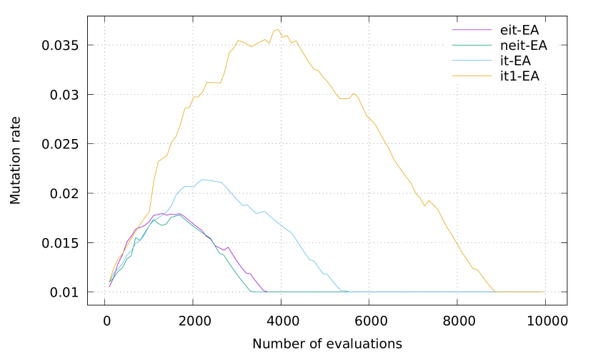
Figure 1: Influence of the update rule on the evolution of the mutation rate. The it-EAs are applied to OneMax with $n=100$, $\lambda=100$, $\mu=1$, $p_{\min}=p_{0}=0.01$, and $\alpha=0.05$.

Fig. 2 shows the influence of the learning rate. The peak increases with the learning rate whereas the width decreases with it.

Figure 2: Influence of the learning rate on the evolution of the mutation rate. The eit-EA is applied to OneMax with $n=100$, $\lambda=100$, $\mu=1$, and $p_{\min}=p_{0}=0.01$. The vertical axis uses a logarithmic scale.

Fig. 3 shows the influence of the number $\mu$ of selected individuals. The value of $\mu$ mostly influences the peak mutation rate. The smaller the value of $\mu$, the larger the peak mutation rate.

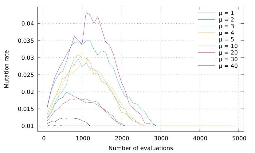
Figure 3: Influence of $\mu$ on the evolution of the mutation rate. The eit-EA is applied to OneMax with $n=100$, $\lambda=100$, $p_{\min}=p_{0}=0.01$, and $\alpha=0.2$.

Fig. 4 shows the influence of the population size $\lambda$. The value of $\lambda$ mostly influences the width of the plot. The larger the value of $\lambda$, the larger the width.

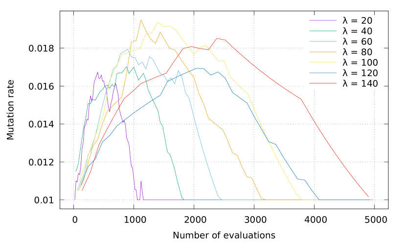
Figure 4: Influence of the population size $\lambda$ on the evolution of the mutation rate. The eit-EA is applied to OneMax with $n=100$, $\mu=1$, $p_{\min}=p_{0}=0.01$, and $\alpha=0.05$.

In the next series of experiments, we study the convergence of the mutation rate under the IGO update alone. To this end, we use Algorithm 1 except that we do not update the center in the loop. We apply this static search to OneMax starting from random bit vectors with different Hamming weights. Instead of the mutation rate $p$ itself, we represent $\theta=\operatorname*{logit}(p)$ in order to better visualize the range of asymptotic values. Fig. 5 shows that the mutation rate converges to asymptotic values closely related to the Hamming weights of initial bit vectors. The larger the Hamming weight, the smaller the asymptotic mutation rate. In particular, for a 100-bit vector of Hamming weight 50, $\theta$ converges to 0 or, equivalently, $p$ converges to $1/2$. The symmetry of Hamming weights about 50 is mapped onto the symmetry of $\theta$ values about 0.

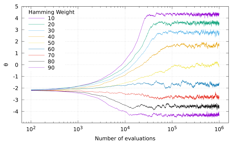
Figure 5: Evolution of $\theta=\operatorname*{logit}(p)$ in static searches starting from random bit vectors of different Hamming weights. The it-EA is applied to OneMax with $n=100$, $\lambda=100$, $\mu=1$, $p_{0}=0.1$, $p_{\min}=0$, $p_{\max}=1$, and $\alpha=0.05$. The horizontal axis uses a logarithmic scale.

8.2 Fixed-target analysis

In the next series of experiments, we study the empirical runtime (number of function evaluations until the maximum is found) of the $(1+\lambda)$ EA, the 2-rate $(1+\lambda)$ EA [12], the eit-EA, and the neit-EA. The it-EA and it1-EA have proved slower than the $(1+\lambda)$ EA and have not been included in the study. For all algorithms, $\lambda=n/10$. For the eit-EA and the neit-EA, $p_{\min}=p_{0}=1/n$ and $\alpha=0.2$. For the 2-rate $(1+\lambda)$ EA, $p_{0}=1/n$, which corresponds to $r^{\text{init}}=1$ in [12].

Fig. 6 shows the mean runtime on OneMax in dimensions up to $n=\numprint{10000}$ (100 runs). The eit-EA and neit-EA with $\mu=1$ have similar performance. Both are faster than the eit-EA with $\mu=n/100$ which, in turn, is faster than the $(1+\lambda)$ EA. The 2-rate $(1+\lambda)$ EA is slower than the eit-EA with $\mu=n/100$ up to $n=\numprint{10000}$ but data suggests that it is faster past a certain dimension. The ratio of the runtime of the 2-rate $(1+\lambda)$ EA and that of the neit-EA with $\mu=1$ is slowly decreasing with $n$ and is approximately equal to 1.22 when $n=\numprint{10000}$. It is an open problem whether the eit-EA or the neit-EA with $\mu=1$ matches the optimal bound of the 2-rate $(1+\lambda)$ EA.

Fig. 7 shows the standard deviation of the runtime on OneMax. It increases faster with the 2-rate $(1+\lambda)$ EA than with the other algorithms in the study. One explanation could be that, at each iteration, the 2-rate $(1+\lambda)$ EA multiplies or divides the mutation rate by two, each with probability $1/4$. In contrast, in the it-EA, the change in the mutation rate implied by Eq. (8) is smooth.

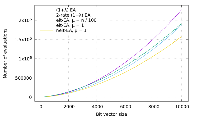
Figure 6: Mean runtime on OneMax as a function of $n$ (100 runs).

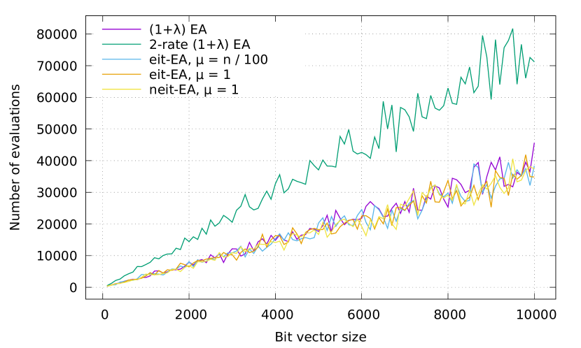
Figure 7: Standard deviation of the runtime on OneMax as a function of $n$ (100 runs).

Fig. 8 shows the mean runtime on LeadingOnes in dimensions up to $n=\numprint{5000}$ (100 runs). The 2-rate $(1+\lambda)$ EA is slower than the other algorithms in the study. The eit-EA and neit-EA with $\mu=1$ are marginally faster than the $(1+\lambda)$ EA. The standard deviation of the runtime on LeadingOnes increases faster with the 2-rate $(1+\lambda)$ EA than with the other algorithms in the study (not shown).

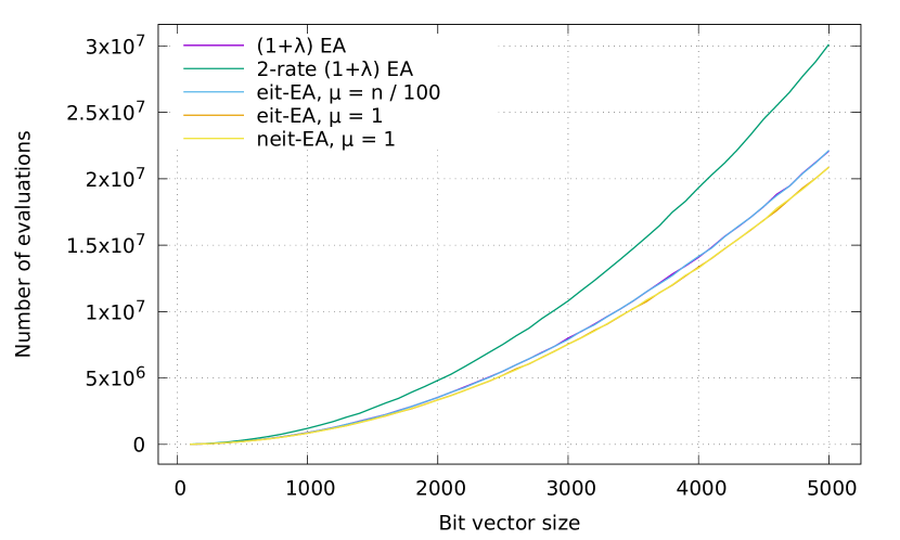
Figure 8: Mean runtime on LeadingOnes as a function of $n$ (100 runs). The $(1+\lambda)$ EA and the eit-EA with $\mu=n/100$ have approximately the same runtime.

9 Conclusion

We have presented a novel evolutionary algorithm on bit vectors, the information theoretic evolutionary algorithm (it-EA). It relies on standard bit mutation and rank-based selection and is completely expressed in terms of information theory. The mutation rate is controlled by means of information-geometric optimization. The IGO update has a clear interpretation in terms of frequency of mutated bits in selected individuals. The center of the search distribution is updated by means of a maximum likelihood principle. The ML update can be interpreted as a multi-parent cross-over operator. The it1-EA with local ML update can be seen as the analogue of CMA-ES for bit vectors, albeit with fewer parameters. We have also considered elitist (eit-EA) and non elitist (neit-EA) selection for replacement.

A series of experiments involving the it-EAs has shown that the IGO update for the mutation rate is effective. An empirical runtime analysis has shown that, on OneMax in dimensions up to $n=\numprint{10000}$, the eit-EA and the neit-EA with $\mu=1$ are faster than the $(1+\lambda)$ EA and even the 2-rate $(1+\lambda)$ EA. On LeadingOnes in dimensions up to $n=\numprint{5000}$, they are marginally faster than the $(1+\lambda)$ EA.

As future work, we plan to evaluate the performance of the it-EAs on test functions other than OneMax and LeadingOnes. In particular, the influence of hyperparameters on performance should be investigated. The theoretical expected runtime of the eit-EA and the neit-EA on OneMax is an interesting open question. Beyond the it-EA, the IGO update (control of the mutation rate) and the ML update (multi-parent cross-over) could find their way into other random search heuristics on bit vectors. More generally, the relation between optimization and learning could be deepened with the help of information theory.

References

- [1] Aldeida Aleti and Irene Moser. A systematic literature review of adaptive parameter control methods for evolutionary algorithms. ACM Computing Surveys (CSUR), 49(3):1–35, 2016.
- [2] Shun-Ichi Amari. Natural gradient works efficiently in learning. Neural Comput., 10(2):251–276, feb 1998.
- [3] Thomas Back. The interaction of mutation rate, selection, and self-adaptation within a genetic algorithm. In Proc. 2nd Conference of Parallel Problem Solving from Nature, 1992. Elsevier Science Publishers, 1992.
- [4] Shumeet Baluja and Rich Caruana. Removing the genetics from the standard genetic algorithm. In Armand Prieditis and Stuart Russell, editors, Proc. of the 12th Annual Conf. on Machine Learning, pages 38–46. Morgan Kaufmann, 1995.
- [5] Arnaud Berny. Selection and reinforcement learning for combinatorial optimization. In International Conference on Parallel Problem Solving from Nature, pages 601–610. Springer, 2000.
- [6] J. S. De Bonet, C. L. Isbell, and P. Viola. MIMIC: finding optima by estimating probability densities. In Advances in Neural Information Processing Systems, volume 9. MIT Press, Denver, 1996.
- [7] Luis DaCosta, Alvaro Fialho, Marc Schoenauer, and Michèle Sebag. Adaptive operator selection with dynamic multi-armed bandits. In Proceedings of the 10th Annual Conference on Genetic and Evolutionary Computation, GECCO ’08, pages 913–920, New York, NY, USA, 2008. Association for Computing Machinery.
- [8] Pieter-Tjerk De Boer, Dirk P Kroese, Shie Mannor, and Reuven Y Rubinstein. A tutorial on the cross-entropy method. Annals of operations research, 134(1):19–67, 2005.
- [9] Benjamin Doerr and Carola Doerr. Theory of parameter control for discrete black-box optimization: Provable performance gains through dynamic parameter choices. In Benjamin Doerr and Frank Neumann, editors, Theory of Evolutionary Computation: Recent Developments in Discrete Optimization, pages 271–321. Springer International Publishing, Cham, 2020.
- [10] Benjamin Doerr, Carola Doerr, and Johannes Lengler. Self-adjusting mutation rates with provably optimal success rules. Algorithmica, pages 1–40, 2021.
- [11] Benjamin Doerr, Carola Doerr, and Jing Yang. k-bit mutation with self-adjusting k outperforms standard bit mutation. In Julia Handl, Emma Hart, Peter R. Lewis, Manuel López-Ibáñez, Gabriela Ochoa, and Ben Paechter, editors, Parallel Problem Solving from Nature – PPSN XIV, pages 824–834, Cham, 2016. Springer International Publishing.
- [12] Benjamin Doerr, Christian Gießen, Carsten Witt, and Jing Yang. The evolutionary algorithm with self-adjusting mutation rate. In Proceedings of the Genetic and Evolutionary Computation Conference, GECCO ’17, pages 1351–1358, New York, NY, USA, 2017. Association for Computing Machinery.
- [13] Nikolaus Hansen and Andreas Ostermeier. Adapting arbitrary normal mutation distributions in evolution strategies: The covariance matrix adaptation. In Proceedings of IEEE international conference on evolutionary computation, pages 312–317. IEEE, 1996.
- [14] Nikolaus Hansen and Andreas Ostermeier. Completely derandomized self-adaptation in evolution strategies. Evolutionary computation, 9(2):159–195, 2001.
- [15] Mark Hauschild and Martin Pelikan. An introduction and survey of estimation of distribution algorithms. Swarm and evolutionary computation, 1(3):111–128, 2011.
- [16] HNCO. https://github.com/courros/hnco. v0.22.
- [17] Giorgos Karafotias, Agoston Endre Eiben, and Mark Hoogendoorn. Generic parameter control with reinforcement learning. In Proceedings of the 2014 Annual Conference on Genetic and Evolutionary Computation, GECCO ’14, pages 1319–1326, New York, NY, USA, 2014. Association for Computing Machinery.
- [18] Giorgos Karafotias, Mark Hoogendoorn, and A. E. Eiben. Parameter control in evolutionary algorithms: Trends and challenges. IEEE Transactions on Evolutionary Computation, 19(2):167–187, 2015.
- [19] S. Kullback. Information theory and statistics. Dover, 1968.
- [20] Pedro Larrañaga and Jose A Lozano. Estimation of distribution algorithms: A new tool for evolutionary computation, volume 2. Springer Science & Business Media, 2001.
- [21] Luigi Malagò, Matteo Matteucci, and Bernardo Dal Seno. An information geometry perspective on estimation of distribution algorithms: Boundary analysis. In Proceedings of the 10th Annual Conference Companion on Genetic and Evolutionary Computation, GECCO ’08, pages 2081–2088, New York, NY, USA, 2008. Association for Computing Machinery.
- [22] Luigi Malagò, Matteo Matteucci, and Giovanni Pistone. Towards the geometry of estimation of distribution algorithms based on the exponential family. In Proceedings of the 11th Workshop Proceedings on Foundations of Genetic Algorithms, FOGA ’11, pages 230–242, New York, NY, USA, 2011. Association for Computing Machinery.
- [23] Heinz Mühlenbein. The equation for response to selection and its use for prediction. Evolutionary Computation, 5(3):303–346, 1997.
- [24] Yann Ollivier, Ludovic Arnold, Anne Auger, and Nikolaus Hansen. Information-geometric optimization algorithms: A unifying picture via invariance principles. J. Mach. Learn. Res., 18(1):564–628, 2017.
- [25] Ingo Rechenberg. Evolutionsstrategie, volume 15 of problemata, 1973.
- [26] Reuven Rubinstein. The cross-entropy method for combinatorial and continuous optimization. Methodology and computing in applied probability, 1(2):127–190, 1999.
- [27] Dirk Thierens. An adaptive pursuit strategy for allocating operator probabilities. In Proceedings of the 7th annual conference on Genetic and evolutionary computation, pages 1539–1546, 2005.
- [28] Marc Toussaint. Notes on information geometry and evolutionary processes. arXiv preprint nlin/0408040, 2004.
- [29] Daan Wierstra, Tom Schaul, Tobias Glasmachers, Yi Sun, Jan Peters, and Jürgen Schmidhuber. Natural evolution strategies. The Journal of Machine Learning Research, 15(1):949–980, 2014.
- [30] Daan Wierstra, Tom Schaul, Jan Peters, and Juergen Schmidhuber. Natural evolution strategies. In 2008 IEEE Congress on Evolutionary Computation (IEEE World Congress on Computational Intelligence), pages 3381–3387, 2008.