Optimizing Sensor Allocation against Attackers with Uncertain Intentions: A Worst-Case Regret Minimization Approach

Abstract

This paper focuses on the optimal allocation of multi-stage attacks with the uncertainty in attacker’s intention. We model the attack planning problem using a Markov decision process and characterize the uncertainty in the attacker’s intention using a finite set of reward functions—each reward represents a type of attacker. Based on this modeling, we employ the paradigm of the worst-case absolute regret minimization from robust game theory and develop mixed-integer linear program (MILP) formulations for solving the worst-case regret minimizing sensor allocation strategies for two classes of attack-defend interactions: one where the defender and attacker engage in a zero-sum game and another where they engage in a non-zero-sum game. We demonstrate the effectiveness of our algorithm using a stochastic gridworld example.

Markov process, Game theory, Optimization

1 Introduction

With the increasing severity of cyber- and physical- attacks, developing effective proactive defense aims to enable early detection of attacks by strategically allocating sensors/intrusion detectors. However, this task is complicated by the fact that attackers often have varying objectives and intentions. This paper studies the design of a robust proactive sensor allocation, given the uncertainty in the objective or the intention of the attacker. Our approach is motivated by real-world cyber security incidents, where defenders have limited monitoring resources and must deal with attackers with different objectives, ranging from using a botnet to interrupt services with a DDoS attack, distributing malware to steal sensitive data, or privilege escalation attacks (see[18], a report on recent cyber security incidents).

We formulate the attack planning problem as a Markov decision process (MDP) and enable the defender to allocate intrusion detectors, called sensors in this context, to detect the presence of an attack. The sensor allocation modifies the transition function of the attack MDP. Specifically, when a state is allocated with a sensor, it becomes a sink/absorbing state, as the attack terminates once a sensor state is reached. Therefore, the goal of designing an optimal sensor allocation is to modify the transition function of the attack MDP such that the attacker’s value can be minimized given the best response attack strategy. The sensor allocation problem in attack graphs[4] is closely related to Stochastic Stackelberg Game (SSG) [16]. In an SSG, the defender/leader commits to a strategy first to protect a set of targets with limited resources, while the attacker/follower selects the best response attack strategy to the defender’s strategy. Related to SSG for sensor allocation, Li et al. [6] developed a mixed-integer linear program (MILP) formulation for solving joint allocation of detectors and stealthy sensors that minimizes the attacker’s probability of success. Sengupta et al. [14] modeled the attacker-defender interaction using a normal-form game and proposed a mixed strategy for the defender to randomize intrusion detectors. Besides the security game, other resource allocation problems have been extensively studied. These include distributing preventive resources to contain the spreading process [9] in a network; allocating sensors for maximizing coverage [7]. The main difference is that in game-theoretic resource allocation, the decision maker’s objective function is a function of the allocated resource and the best response of the attacker, which can be influenced by how the sensors are allocated.

Traditional Stackelberg security games assume that the defender knows the attacker’s payoff function, which is often not the case. To address this, researchers have studied robust defense design from the perspective of robust optimization [1]. In [10], the authors considered robust Stackelberg equilibria in normal form games where the uncertainty comes from multiple $\epsilon$-optimal best responses from the follower. In [17], the authors used an MDP to model the attack planning problem and employed robust optimization to design a moving target defense (MTD) policy that is robust to a finite uncertainty set of attack strategies. In [5], the authors introduced a robust Stackelberg equilibrium that maximizes the leader’s payoff given the worst-case realization of the follower’s payoff in a deterministic sequential game in which each player selects a distribution over action sequences. The uncertainty is assumed to lie within a bounded interval on the follower’s payoff.

Similar to [5], we also investigate the problem of robust defense when the defender has incomplete knowledge about the attacker’s payoffs, modeled as a finite set of attacker’s types. Each type is associated with a unique reward function that describes the attack objective. We consider robust sensor allocation with the solution of the worst-case absolute regret minimization [11].

The proposed Worst-Case Absolute Regret Minimization for Sensor Allocation (WCARM-SA) solution informs a regret-averse defender to choose a strategy that leads to a small regret once he realizes what would have been the best decision if he knew the attacker’s type. As shown in operations research, the WCARM-SA solutions are often less conservative solutions compared to those by robust optimization [13, 11].

Our contribution can be summarized as:

• We develop WCARM-SA methods to solve robust sensor allocation problems in zero-sum and non-zero-sum attack-defend interactions with uncertainty in the attack intention, described by a finite set of possible attacker’s reward functions. We demonstrate that the WCARM-SA can be formulated as MILP problems for both cases.

• We leverage the zero-sum property to develop efficient solution for the WCARM-SA for the zero-sum case.

• We validate the effectiveness of our proposed approach through experiments with attack motion planning problems in stochastic gridworld environments.

2 Preliminaries and Problem Formulation

Notations Let $\mathbf{R}$ denote the set of real numbers and $\mathbf{R}^{n}$ the set of real $n$-vectors. The vector of all ones is represented as $\mathbf{1}$. The notation $z_{i}$ refers to the $i$-th component of a vector $z\in\mathbf{R}^{n}$ or to the $i$-th element of a sequence $z_{1},z_{2},\ldots$, which will be clarified by the context. The set of probability distributions over a finite set $Z$ is denoted as $\mathsf{Dist}(Z)$.

We begin by presenting an attack MDP that captures an attacker’s planning problem.

Attack Planning Problem The attack planning problem is modeled as an attack MDP $M=(S,A,P,\nu,\gamma,R),$ where $S$ is a set of states (nodes in the attack graph) including a special absorbing/sink state $s_{\mathsf{sink}}$, $A$ is a set of attack actions, $P:S\times A\rightarrow\mathsf{Dist}(S)$ is a probabilistic transition function such that $P(s^{\prime}|s,a)$ is the probability of reaching state $s^{\prime}$ given action $a$ being taken at state $s$, $\nu\in\mathsf{Dist}(S)$ is the initial state distribution, $\gamma\in(0,1]$ is a discount factor, and $R:S\times A\rightarrow\mathbf{R}$ is the attacker’s reward function such that $R(s,a)$ is the reward received by the attacker for taking action $a$ in state $s$. The attacker’s objective is to maximize the total discounted rewards in the attack MDP. For concrete examples of attack graphs generated from network vulnerabilities, readers are directed to [4] and [6].

We consider Markovian policies because it suffices to search in Markovian policies for an optimal policy in the attack MDP[12]. Given a Markovian policy $\pi\colon S\to\mathsf{Dist}(A)$, the attacker’s value function $V_{2}^{\pi}:S\rightarrow\mathbf{R}$ is defined as

$$V_{2}^{\pi}(s)=E_{\pi}[\sum\limits_{k=0}^{\infty}\gamma^{k}R(s_{k},\pi(s_{k}))|s_{0}=s],$$

where $E_{\pi}$ is the expectation and $s_{k}$ is the $k$-th state in the Markov chain induced from the MDP $M$ under the policy $\pi$, starting from state $s$. The attacker’s value given the initial distribution $\mu$ is $V_{2}^{\pi}(\mu)=\sum_{s\in S}\mu(s)V_{2}^{\pi}(s).$

Defender’s incomplete information The defender knows the dynamics in the attack MDP. However, the defender does not know the exact reward function of the attacker; rather, the defender is only aware that the attacker can fall into one attack type at any given time. Different attacker types only differ in their reward function in the attack MDP and share the same states, actions, transition function, initial distribution, and discount factor. Specifically, let $\mathcal{T}=\{1,\ldots,N\}$ be the attacker’s type space. Let $R_{i}:S\times A\rightarrow\mathbf{R}$ be the reward function for attacker type $i$.

Defender’s countermeasures To detect an ongoing attack, the defender is capable of allocating sensors to a subset $U\subset S$ of states in the MDP $M$. The attack will be terminated immediately once the attacker reaches a state monitored by the sensor (assuming the sensor’s false negative rate is 0) . However, the defender’s sensor allocation is constrained. Specifically, we consider a sensor allocation as a Boolean vector $\vec{x}\in\{0,1\}^{\lvert S\rvert}$. If $\vec{x}(s)=1$, then the state $s\in U$ is allocated with a sensor. A valid allocation $\vec{x}$ needs to satisfy $\vec{x}(s)=0$ for any $s\in S\setminus U$ because only states in $U$ can be monitored. In addition, the number of sensors cannot exceed a given integer $k$, i.e., $\mathbf{1}^{\mathsf{T}}\vec{x}\leq k$.

We state the problem informally as follows.

Problem 1.

In the attack planning modeled as the MDP $M$ with uncertainty in the attacker’s type, how to robustly allocate limited sensors with respect to the defense objective?

3 Main Results

First, it is observed that a sensor allocation changes the transition function of the attack MDP as follows.

Definition 1 (Attack MDP equipped with sensors).

Given a sensor allocation $\vec{x}$ and the original attack MDP $M=(S,A,P,\nu,\gamma,R)$, the attack MDP under $\vec{x}$ is the MDP

$$M(\vec{x})=(S,A,P^{\vec{x}},\nu,\gamma,R),$$

where $S,A,\nu,\gamma,R$ are identical to those in $M$, and $P^{\vec{x}}$ is defined as

$$P^{\vec{x}}(s^{\prime}|s,a)=\begin{cases}1,&\vec{x}(s)=1,\ s^{\prime}=s_{\mathsf{sink}},\\ 0,&\vec{x}(s)=1,\ s^{\prime}\neq s_{\mathsf{sink}},\\ P(s^{\prime}|s,a),&\vec{x}(s)=0.\end{cases}$$

To allocate sensors with uncertainty in the attacker’s type, we employ a solution of robust game [11, 15], called worst-case absolute regret minimization, which optimizes the performance of a decision variable, $\vec{x}$ in our context, with respect to the “worst-case regret” that might be experienced when comparing $\vec{x}$ to the best decision that should have been made given the attacker’s type $i$ is known. Next, we discuss two approaches to solve worst-case regret minimizing sensor allocations given i) Zero-sum attack-defend game: For each attack type $i$, the defender’s value in $M(\vec{x})$ is the negation of the attacker $i$’s value. ii) Non-zero-sum attack-defend game: Regardless of the attacker’s type, the defender’s value in $M(\vec{x})$ is defined by evaluating the attacker’s strategy with respect to a defender’s cost function $C:S\times A\rightarrow\mathbf{R}$. The defender’s goal is to minimize the total discounted costs respecting $C$ incurred by the attacker’s strategy.

3.1 Worst-case regret minimization in zero-sum game

In the zero-sum case, it is first noted that the optimal sensor allocation $\vec{x}_{i}$ for attacker’s type $i$ can be obtained by solving the following optimization problem:

$$\vec{x}_{i}=\arg\min_{\vec{x}\in\mathcal{X}}\max_{\pi}V_{2,i}^{\pi}(\nu;\vec{x}).$$

where $V_{2,i}^{\pi}(\nu;\vec{x})$ is attacker $i$’s value given attack strategy $\pi$ in the MDP $M(\vec{x})$ and the attacker $i$’s reward $R_{i}$. The optimal sensor allocation problem can be formulated as an MILP (see [6]). As a result, the WCARM-SA problem is formulated as:

$$(\mbox{\acs{wcarm}})\mbox{minimize}_{\vec{x}\in\mathcal{X}}\max_{i\in\mathcal{T}}\left(V_{2,i}(\vec{x})-V_{2,i}(\vec{x}_{i})\right)$$

where $V_{2,i}(\vec{z})=\max_{\pi}V_{2,i}^{\pi}(\nu,\vec{z})$ for $z=\vec{x},\vec{x}_{i}$. That is, the attacker always chooses the optimal strategy in MDP $M(\vec{x})$. The difference $V_{2,i}(\vec{x})-V_{2,i}(\vec{x}_{i})$ measures the regret of the defender for choosing $\vec{x}$ instead of $\vec{x}_{i}$ when the attacker is type $i$. The regret is always non-negative for any sensor allocation decision $\vec{x}\in\mathcal{X}$ because $\vec{x}_{i}=\arg\min_{\vec{x}}V_{2,i}(\vec{x})$.

Because $\vec{x}_{i}$ is pre-computed for each attacker type, the quantity $V_{2,i}(\vec{x_{i}})$ is a constant, denoted by $v_{i}$ for clarity. The optimization problem is then written as:

$$\quad\mbox{minimize}_{\vec{x}\in\mathcal{X}}\max_{i\in\mathcal{T}}\left(V_{2,i}(\vec{x})-v_{i}\right),$$

which is a robust optimization problem. The following lemma shows how the robust optimization problem can be reformulated as an MILP.

Lemma 1.

The worst-case absolute regret minimization problem for robust sensor allocation in a zero-sum game is equivalent to the following optimization problem:

$$\operatorname*{\textrm{min.}}_{y,\vec{x}\in\mathcal{X}} \quad y$$ (1)

$$\operatorname*{\textrm{s.t.}} y\geq V_{2,i}(\vec{x})-v_{i},\forall i\in\mathcal{T},$$ (2)

$$V_{2,i}(\vec{x})=\sum_{s\in S}\nu(s)V_{2,i}(s;\vec{x}),\forall i\in\mathcal{T},$$ (3)

$$V_{2,i}(s;\vec{x})\geq R_{i}(s,a)+\gamma\sum_{s^{\prime}}P^{\vec{x}}(s^{\prime}|s,a)V_{2,i}(s^{\prime};\vec{x}),$$

$$\forall s\in S,\forall a\in A,\forall i\in\mathcal{T},$$ (4)

$$\mathbf{1}^{\mathsf{T}}\vec{x}\leq k.$$ (5)

Proof.

For attacker type $i$ and a sensor design $\vec{x}$, the optimal attacker’s value vector, denoted $V^{\ast}_{2,i}(\vec{x})\in\mathbf{R}^{\lvert S\rvert}$ satisfies the Bellman optimality condition: For all $s\in S$,

$$V^{\ast}_{2,i}(s,\vec{x})=\max_{a\in A}\left(R_{i}(s,a)+\gamma\sum_{s^{\prime}\in S}P^{\vec{x}}(s^{\prime}|s,a)V^{\ast}_{2,i}(s^{\prime};\vec{x})\right).$$

Based on the linear program formulation of dynamic programming [2], any vector $V_{2,i}(\vec{x})$ satisfying the set of constraints in (4) is an upper bound on the $V^{\ast}_{2,i}(\vec{x})$, for all $s\in S$ element-wise. Therefore, $\sum_{s\in S}\nu(s)V_{2,i}(s;\vec{x})\geq\sum_{s\in S}\nu(s)V^{\ast}_{2,i}(s;\vec{x})$. Constraints (2), (3), and (4) together enforce $y\geq\max_{i\in\mathcal{T}}(\sum_{s\in S}\nu(s)V_{2,i}(s;\vec{x})-v_{i})\geq\max_{i\in\mathcal{T}}(V^{\ast}_{2,i}(\nu;\vec{x})-v_{i})$.

For an arbitrary $\vec{x}$, let $r(\vec{x})=\mathop{\mathrm{argmax}}_{i\in\mathcal{T}}(V^{\ast}_{2,i}(\nu;\vec{x})-v_{i})$, that is, the $r(\vec{x})$ is the attacker type for which the defender’s regret of using $\vec{x}$ is the largest among the regret for all attacker’s types. Then we have $y\geq\max_{i\in\mathcal{T}}(V^{\ast}_{2,i}(\nu;\vec{x})-v_{i})=V^{\ast}_{r(\vec{x})}(\nu;\vec{x})-v_{r(\vec{x})}$. Because $v_{r(\vec{x})}$ is a constant once ${r(\vec{x})}$ is determined, minimizing $y$ is equivalent to minimizing the upper bound of $V_{r(\vec{x})}(\nu;\vec{x})$ and thus $y=V^{\ast}_{r(\vec{x})}(\nu;\vec{x})-v_{r(\vec{x})}$. The optimization problem is then $\min_{\vec{x}}(V^{\ast}_{r(\vec{x})}(\nu;\vec{x})-v_{r(\vec{x})})$, which is equivalent to the WCARM-SA formulation. ∎

It is noted that the optimization problem in (1) is nonlinear because the transition function $P^{\vec{x}}$ depends on the decision variable $\vec{x}$ and the constraints in (4) include product terms between the transition probabilities with the other variable $V_{2,i}(s,\vec{x})$. We show how to transform the nonlinear program into an MILP next.

By the definition of $P^{\vec{x}}$ in (• ‣ 2), the term $\sum_{s^{\prime}}P^{\vec{x}}(s^{\prime}|s,a)V_{2,i}(s^{\prime};\vec{x})$ in (5) satisfies

$$\sum_{s^{\prime}}P^{\vec{x}}(s^{\prime}|s,a)V_{2,i}(s^{\prime};\vec{x})$$

$$\quad=\begin{cases}V_{2,i}(s_{\mathsf{sink}};\vec{x}),&\vec{x}(s)=1,\\ \sum_{s^{\prime}}P(s^{\prime}|s,a)V_{2,i}(s^{\prime};\vec{x}),&\vec{x}(s)=0\end{cases}$$

$$\quad=\sum_{s^{\prime}}P(s^{\prime}|s,a)V_{2,i}(s^{\prime};\vec{x})(1-\vec{x}(s))+V_{2}(s_{\mathsf{sink}};\vec{x})\vec{x}(s)$$

$$\quad=\sum_{s^{\prime}}P(s^{\prime}|s,a)V_{2,i}(s^{\prime};\vec{x})(1-\vec{x}(s)),$$

where the last equality is implied by $V_{2}(s_{\mathsf{sink}};\vec{x})=0$. Define

Using the big-M method [3], Eq. (6) can be expressed equivalently as affine inequalities (in $\vec{x}$, $V_{2,i}$, and $W_{2,i}$)

$$W_{2,i}(s,s^{\prime})\leq M(1-\vec{x}(s)),$$ (7)

$$W_{2,i}(s,s^{\prime})\geq m(1-\vec{x}(s)),$$ (8)

$$W_{2,i}(s,s^{\prime})-V_{2,i}(s^{\prime};\vec{x})\leq M\vec{x}(s),$$ (9)

$$W_{2,i}(s,s^{\prime})-V_{2,i}(s^{\prime};\vec{x})\geq m\vec{x}(s).$$ (10)

with proper choices of constants $M>0$ and $m<0$. For example, let $M$ be the upper bound on the total rewards and $m$ be the negation of the upper bound on the total rewards.

3.2 Worst-case regret minimization in non-zero-sum game

Next, we consider the scenario where the defender aims to minimize her cost function $C:S\times A\rightarrow\mathbf{R}$, which maps a state and an attack action to a cost penalty that measures the loss incurred by the attacker’s action. Because the penalty is not necessarily the negation of the attack reward, the attack-defend game is non-zero-sum. For a single type of attacker, we formulate the problem as a Stackelberg game as follows.

Definition 2.

For a single type of attacker whose attack MDP is $M=(S,A,P,\mu,\gamma,R)$, and the defender’s capability of allocating sensors, an SSG is formulated as a tuple $G=(S,A_{1},A_{2},\mathcal{P},\nu,\gamma,R_{1},R_{2}),$ where

• $S$, $\nu$, $\gamma$ are the same components in the attack MDP $M$ for states, initial distribution, and discount factor.

• $A_{1}=\{0,1\}$ is the defender/leader’s action set. Action $0$ for not allocating a sensor, 1 for allocating a sensor.

• $A_{2}=A$ is the attacker/follower’s actions.

• $\mathcal{P}(s^{\prime}|s,a_{1},a_{2})$ is the probability of reaching state $s^{\prime}$ given action $a_{1},a_{2}$ being taken by the defender and the attacker at state $s$. For a state $s\in S$, a defender’s action $a_{1}\in A_{1}$ and an attacker’s action $a_{2}\in A_{2}$, let

  $$\mathcal{P}(s^{\prime}|s,a_{1},a_{2})=\begin{cases}1,&a_{1}=1,\ s^{\prime}=s_{\mathsf{sink}},\\ 0,&a_{1}=1,\ s^{\prime}\neq s_{\mathsf{sink}},\\ P(s^{\prime}|s,a_{2}),&a_{1}=0.\end{cases}$$

• $R_{1}:S\times A_{1}\times A_{2}\rightarrow\mathbf{R}$ (resp. $R_{2}:S\times A_{1}\times A_{2}\rightarrow\mathbf{R}$) is the leader(resp. follower)’s reward function, defined with the defender’s cost $C$ (resp. the attacker’s reward $R$):

  $$R_{1}(s,a_{1},a_{2})=\begin{cases}0,&a_{1}=1,\\ -C(s,a_{2}),&a_{1}=0,\\ \end{cases}$$

  $$R_{2}(s,a_{1},a_{2})=\begin{cases}0,&a_{1}=1,\\ R(s,a_{2}),&a_{1}=0.\\ \end{cases}$$

In this SSG, the defender/leader decides the sensor allocation, which determines the transition function $\mathcal{P}$. The attacker/follower decides on the best response to maximize his reward. The reward function is understood as follows: When the defender allocates a sensor to state $s$ (i.e., $a_{1}=1$), the attack terminates in that state, and no further costs/rewards will be incurred for either player. Otherwise (i.e., $a_{1}=0$), the attacker continues to reach the next state with action $a_{2}$, and both the defender and the attacker receive a reward of $-C(s,a_{2})$ and $R(s,a_{2})$, respectively. In this formulated SSG, both the defender and the attacker aim to maximize their respective total discounted rewards.

Since sensors cannot be moved once allocated, we restrict the defender’s strategy to be deterministic and memoryless. Given a fixed sensor allocation, the best response attack strategy can also be deterministic. For a strategy profile $(\pi_{1},\pi_{2})$–a tuple of the defender’s strategy $\pi_{1}:S\rightarrow A_{1}$ and $\pi_{2}:S\rightarrow A_{2}$, the defender’s value function $V_{1}$ is defined as

where the expectation is taken in the Markov chain induced from $G$ given the strategy profile $(\pi_{1},\pi_{2})$.

For the non-zero-sum case, the WCARM-SA problem takes the following form:

$$(\mbox{\acs{wcarm}})\mbox{minimize}_{\pi_{1}}\max_{i\in\mathcal{T}}\left(V_{1,i}(\nu,\pi_{1}^{i})-V_{1,i}(\nu,\pi_{1})\right),$$

where $V_{1,i}(\nu,\pi_{1}^{i})$ is the defender’s value given both the defender and the attacker committing to the Stackelberg equilibrium in the SSG $G$ (Def. 2) where the attacker’s reward $R_{2}$ is defined based on the reward function of attack type $i$. The Stackelberg equilibrium can be solved with methods in [19], with a modification that constrains the defender’s strategy to be deterministic. The regret $V_{1,i}(\nu,\pi_{1}^{i})-V_{1,i}(\nu,\pi_{1})$ measures the defender’s regret in using strategy $\pi_{1}$ against attacker $i$ to the defender’s best strategy $\pi_{1}^{i}$ that should have been employed when playing against attacker $i$.

To find $\pi_{1}^{\ast}$ that minimizes the worst-case regret, we introduce a decision variable $y$ and rewrite the optimization problem as follows:

$$\operatorname*{\textrm{min.}}_{\pi_{1}} \quad y$$ (11)

$$\operatorname*{\textrm{s.t.}} y\geq V_{1,i}(\nu,\pi_{1}^{i})-V_{1,i}(\nu,\pi_{1}),\forall i\in\mathcal{T},$$ (12)

where $V_{1,i}(\nu,\pi_{1}^{i})$ is a constant and is denoted by $\bar{v}_{1,i}$.

We extend the MILP formulation in [19] and get the following mixed-integer nonlinear program (MINLP) formulation to solve the WCARM-SA problem:

$$\min\limits_{\pi_{1},\{V_{1,i},\pi_{2}^{i},V_{2,i}\mid i\in\mathcal{T}\}}y$$ (13a)

subject to:

$$y\geq\bar{v}_{1,i}-\sum_{s\in S}\nu(s)V_{1,i}(s),\;\;\forall i\in\mathcal{T},$$ (13b)

$$\pi_{1}(a_{1}\mid s)\in\{0,1\},\;\forall s\in S,a_{1}\in\{0,1\},$$ (13c)

$$\sum\limits_{a_{1}\in\{0,1\}}\pi_{1}(a_{1}\mid s)=1\;\;\forall s\in S,$$ (13d)

$$\pi_{2}^{i}(a_{2}\mid s)\in\{0,1\},\;\;\forall i\in\mathcal{T},s\in S,a_{2}\in A,$$ (13e)

$$\sum\limits_{a_{2}\in A}\pi_{2}^{i}(a_{2}\mid s)=1,\;\;\forall i\in\mathcal{T},s\in S,$$ (13f)

$$\sum_{s\in S}\pi_{1}(1|s)\leq k,$$ (13g)

The following constraints hold $$\forall i\in\mathcal{T},s\in S,a_{2}\in A_{2}$$ :

$$(\pi^{i}_{2}(a_{2}\mid s)-1)Z\leq V_{1,i}(s)-\tilde{R}_{1}^{i}(s,\pi_{1},a_{2})$$

$$\leq(1-\pi^{i}_{2}(a_{2}\mid s))Z,$$ (13h)

$$0\leq V_{2,i}(s)-\tilde{R}_{2}^{i}(s,\pi_{1},a_{2})\leq(1-\pi^{i}_{2}(a_{2}\mid s))Z,$$ (13i)

where $\tilde{R}_{1}^{i}(s,\pi_{1},a_{2})=\sum_{a_{1}\in\{0,1\}}\pi_{1}(a_{1}|s)(R_{1}(s,a_{1},a_{2})+\gamma\sum_{s^{\prime}}\mathcal{P}(s^{\prime}|s,a_{1},a_{2})V_{1,i}(s^{\prime}))$ represents the defender’s expected value from state $s$ given the sensor allocation $\pi_{1}$ and attacker’s action $a_{2}$ from state $s$, and the function $\tilde{R}_{2}^{i}(s,\pi_{1},a_{2})$ is defined for the attacker analogously by substituting the defender’s reward and value of the next state with the attacker’s. $Z$ is a large constant number, which can be the upper bound on the absolute value of total rewards.

The constraints in (13) are explained as follows: Constraint (13b) enforces $y$ to be the worst-case regret. Constraint (13c) and (13d) enforce the defender takes a deterministic strategy, constraint (13e), (13f) enforce attacker takes a deterministic strategy. Constraint (13g) enforces the defender can not allocate more than $k$ sensors. Constraint (13) enforces that when the attacker $i$ takes action $a_{2}$, the defender’s value at that state $V_{1,i}(s)$ should equal the expected value $\tilde{R}_{1}^{i}(s,\pi_{1},a_{2})$ of defender against attacker $i$ who takes action $a_{2}$ at state $s$. When the attacker does not take action $a_{2}$, the constraint is non-binding. This set of constraints obtain $V_{1,i}(s)$ by evaluating strategy $\pi_{1}$ at the state $s$ against the attacker’s best response for $\pi_{1}$. Constraint (13i) enforces that when the attacker $i$ takes action $a_{2}$, his value $V_{2,i}(s)$ should be the same as his expected value $\tilde{R}_{2}^{i}(s,\pi_{1},a_{2})$ given that action $a_{2}$. When $a_{2}$ is not taken at $s$, the attacker’s value $V_{2,i}(s)$ should be greater than the expected value $\tilde{R}_{2}^{i}(s,\pi_{1},a_{2})$ due to the fact that $V_{2,i}(s)=\max_{a_{2}}\tilde{R}_{2}^{i}(s,\pi_{1},a_{2})$. By enforcing this constraint, we can ensure $V_{2,i}$ is the attacker’s value given the defender’s strategy $\pi_{1}$ and the attacker’s best response to $\pi_{1}$.

Lemma 2.

The worst-case absolute regret minimization solution for robust sensor allocation in the non-zero-sum attack-defender game is equivalent to the solution of  (13).

The proof is similar to that of Lemma 1 and can be found in the Appendix. The key insight is that constraints (13b), (13i) and(13) together enforce $y\geq\max_{i\in\mathcal{T}}(\bar{v}_{1,i}-\sum_{s\in S}\nu(s)V_{1,i}(s))$ where $V_{1,i}(\cdot)$ is the defender’s value given the best response of attacker type $i$ (enforced by (13)).

The above formulation is nonlinear due to the interaction between the integer variable $\pi_{1}$ and the continuous variable $V_{1,i}$ in $\tilde{R}_{1}^{i}$ ($\tilde{R}_{2}^{i}$ analogously). But since the integer variable is binary, we can use McCormick Relaxation[8] to reformulate MINLP into MILP. To do so, let’s introduce new variables for the defender: for $i\in\mathcal{T},s\in S,a_{1}\in\{0,1\},a_{2}\in A_{2}$, define $w_{s,i}^{a_{1},a_{2}}=\pi_{1}(a_{1}|s)\sum_{s^{\prime}}\mathcal{P}(s^{\prime}|s,a_{1},a_{2})V_{1,i}(s^{\prime})$. Analogously let $z_{s,i}^{a_{1},a_{2}}$ be defined for the attacker.

We then replace $\tilde{R}^{i}_{1}(s,\pi_{1},a_{2})$ in (13) with $\sum_{a_{1}\in\{0,1\}}(\pi_{1}(a_{1}|s)R_{1}(s,a_{1},a_{2})+\gamma w^{a_{1},a_{2}}_{s,i})$ and add the following constraints: $\forall i\in\mathcal{T},s\in S,a_{1}\in\{0,1\},a_{2}\in A$:

$$w_{s,i}^{a_{1},a_{2}}\geq\sum\limits_{s^{\prime}\in S}\mathcal{P}(s^{\prime}|s,a_{1},a_{2})V_{1,i}(s^{\prime})-Z(1-\pi_{1}(a_{1}|s)),$$

$$w_{s,i}^{a_{1},a_{2}}\leq\sum\limits_{s^{\prime}\in S}\mathcal{P}(s^{\prime}|s,a_{1},a_{2})V_{1,i}(s^{\prime})+Z(1-\pi_{1}(a_{1}|s)),$$

$$-Z\cdot\pi_{1}(a_{1}|s)\leq w_{s,i}^{a_{1},a_{2}}\leq Z\cdot\pi_{1}(a_{1}|s).$$

We replace $\tilde{R}^{i}_{2}(s,\pi_{1},a_{2})$ in (13i) and add constraints for $z^{a_{1},a_{2}}_{s,i}$ analogously. For both zero-sum and non-zero-sum cases, the formulated MILP can be solved using the Gurobi Solver.

Remark 1.

If different attackers have different transition functions $P_{i}$, then their corresponding transition functions are used in Constraints (4) for the zero-sum case and in defining $\tilde{R}^{i}_{1}(s,\pi_{1},a_{2})$ and $\tilde{R}^{i}_{2}(s,\pi_{1},a_{2})$ for the non-zero-sum case.

Complexity analysis: Solving an MILP is NP-complete and its runtime complexity depends on the number of constraints and integer variables. In the non-zero-sum case, the number of integer variables required for the WCARM-SA is $O(\lvert S\rvert\times\lvert A_{2}\rvert\times\lvert\mathcal{T}\rvert)$. The number of constraints is $O(\lvert S\rvert\times\lvert A_{1}\rvert\times\lvert A_{2}\rvert\times\lvert\mathcal{T}\rvert)$. For the zero-sum case, the number of integer variables and constraints is $O(\lvert S\rvert)$ and $O(\lvert S\rvert\times\lvert A_{2}\rvert\times\lvert\mathcal{T}\rvert)$ respectively. While the WCARM-SA solution for the non-zero-sum case can be applied to the zero-sum case, the zero-sum case formulation in Sec. 3.1 is more efficient.

4 Experiments

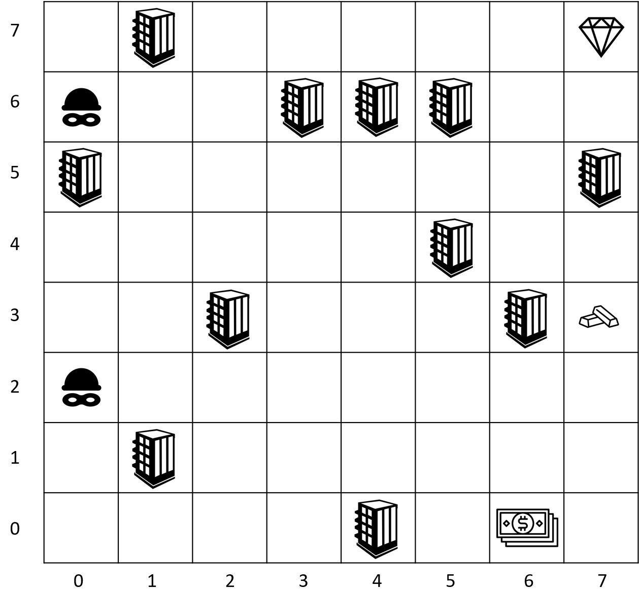
Figure 1: The 8 $\times$ 8 Gridworld Example.

Reward/Cost	Cash (0, 6)	Gold (3, 7)	Diamond (7, 7)
Attacker 1	15	12	12
Attacker 2	12	15	15
Defender	15	10	10

Table 1: Reward functions of two attackers and the cost function of the defender (for the non-zero-sum case).

We used an $8\times 8$ gridworld environment, depicted in Figure 1, to demonstrate our solutions. A state is denoted by $(\mbox{row},\mbox{col})$. There are two types of attackers with the same initial state distribution. Both attackers have a $70\%$ probability of starting from state $(2,0)$ and a $30\%$ probability of starting from state $(6,0)$. Each attacker can move in one of four compass directions. When given the action “N”, the attacker enters the intended cell with a $1-2\alpha$ probability, and enters the neighboring cells, which are the west and east cells, with probability $\alpha$. In our experiment, we set $\alpha=0.1$. If the attacker moves into the buildings or the boundary, he remains in the previous cell. The environment contains three final states, each with a different value for the attackers. The attackers only receive a reward when they reach these final states. Table 1 lists the rewards for the attackers.

First, we consider the worst-case regret minimization in the zero-sum case. We change the number of sensors the defender can allocate to evaluate how sensor numbers affect the defender’s value. As shown in Figure 2, the attacker’s expected value decreases when the sensor number increases.

In the case where only two sensors can be allocated, we compare the robust sensor allocation $\vec{x}^{\ast}$ with the optimal allocation strategies $\vec{x}_{1}$ and $\vec{x}_{2}$ against attacker types $1$ and $2$, respectively. When the defender knows the attacker’s type, $\vec{x}_{1}$ yields a value of $5.96$ for attacker $1$ and $\vec{x}_{2}$ yields a value of $6.56$ for attacker $2$. However, when the defender does not know the attacker’s type and implements $\vec{x}^{\ast}$, the values become $6.12$ and $7.04$ for attackers $1$ and $2$, respectively. In this case, the defender’s worst-case absolute regret is $\max(6.12-5.96,7.04-6.56)=0.48$.

Using $\vec{x}_{1}$ against attacker $2$ results in a regret of $0.89$, while using $\vec{x}_{2}$ against attacker $1$ results in a regret of $1.49$. In both cases, the worst-case regret is higher than that of $\vec{x}^{\ast}$, indicating the advantage of the WCARM-SA method. The WCARM-SA sensor allocations for different numbers of sensors are listed in Table 2 as well as the defender’s worst-case regret under the robust policy. When 4 sensors are allocated, $\vec{x}_{1}=\vec{x}_{2}=\vec{x}^{\ast}=(1,5),(2,5),(5,5),(7,5)$ and the defender’s worst-case regret $y=0$. An attacker is prevented from reaching any final state with probability $1$.

$k$	Policy $\vec{x}_{1}$	Policy $\vec{x}_{2}$	Robust policy $\vec{x}^{\ast}$	$y$
1	$(1,5)$	$(2,2)$	$(2,3)$	$0.22$
2	$(1,5),(2,4)$	$(2,2),(6,2)$	$(1,5)(6,2)$	$0.48$
3	$(1,5),(2,4),(6,2)$	$(2,3)(5,2)(6,2)$	$(1,5),(2,2)(6,2)$	$0.77$

Table 2: Sensor allocation in the zero-sum case. $\vec{x}_{i}$ is the optimal defender policy against attacker type $i\in\{1,2\}$.

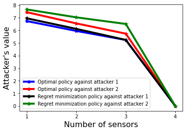
Figure 2: The attacker’s expected value for zero-sum case.

Moving on to the non-zero-sum case, the defender now receives a penalty when the attacker reaches the goal state, and the cost function for the defender is listed in Table 1. The sensor allocation strategies for the non-zero-sum cases, as well as the defender’s worst-case regret under the robust policy, can be found in Table 3. Noted that the worst-case regret is not indicative of the effectiveness of sensor allocations, that is, a small regret does not necessarily mean a large value for the defender. Thus, Figure 3 demonstrates that the defender’s expected value increases as the number of sensors increases. From Fig. 3, it is observed that when two sensors are deployed, the worst-case regret is the largest for both attackers.

Similar to the zero-sum case, when 4 sensors can be allocated, $\vec{x}_{1}=\vec{x}_{2}=\vec{x}^{\ast}=(1,5),(2,5),(5,5),(7,5)$ and the defender’s worst-case regret $y=0$.

$k$	Policy $\pi_{1}$	Policy $\pi_{2}$	Robust Policy $\pi^{\ast}$	$y$
1	$(1,5)$	$(2,2)$	$(2,3)$	$0.26$
2	$(1,5),(2,4)$	$(2,3),(6,2)$	$(1,5),(7,5)$	$1.19$
3	$(1,4),(2,5),(6,2)$	$(2,3),(5,2),(6,2)$	$(1,5),(2,2),(6,2)$	$0.20$

Table 3: Sensor allocation in the non-zero-sum case. $\vec{x}_{i}$ is the optimal defender policy against attacker type $i\in\{1,2\}$.

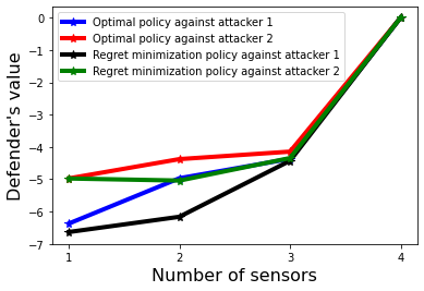
Figure 3: The defender’s expected value.

The experiments are conducted on a Windows 10 machine with Intel(R) i7-11700k CPU and $32$ GB RAM. The computation time for robust sensor allocations in the zero-sum cases is less than 1 second. For non-zero-sum cases, it takes from 77 sec to 3 hours to solve given increasing sensor numbers.

5 Conclusion

We develop robust sensor allocation methods in probabilistic attack planning problems using worst-case absolute regret minimization from robust game theory. We demonstrated that both robust zero-sum and non-zero-sum sensor allocation problems can be formulated as MILPs. Our approach is suitable for a wide range of safety-critical scenarios that involve constructing probabilistic attack graphs from known network vulnerabilities. Future work could focus on developing more efficient and approximate solutions for robust sensor allocations in non-zero-sum games. Additionally, the solution concept for robust games can be extended to design moving target defenses that randomize network topologies and the integrated design of sensor allocation and moving target defense.

Appendix

5.1 Proof of Lemma 2

For attacker type $i$ and a sensor design $\pi_{1}$, constraint (13i) restricts the optimal attacker’s value $V_{2,i}$ satisfies the Bellman optimality condition, and $\pi_{2}^{i}$ is the corresponding optimal policy. Constraint (13) restricts the optimal defender’s value $V_{1,i}$ to satisfy the Bellman optimality condition. Constraints (13b), (13i) and(13) together enforces $y\geq\max_{i\in\mathcal{T}}(\bar{v}_{1,i}-\sum_{s\in S}\nu(s)V_{1,i}(s))$.

The rest of the reasoning follows the same from the zero-sum case and is repeated here for completeness: For an arbitrary $\pi_{1}$, let $r(\pi_{1})=\mathop{\mathrm{argmax}}_{i\in\mathcal{T}}(\bar{v}_{1,i}-\sum_{s\in S}\nu(s)V_{1,i}(s))$, that is the $r(\pi_{1})$ is the attacker type for which the defender’s regret of using sensor design $\pi_{1}$ is the largest among the regret for all attacker’s types. Then we have $y\geq\max_{i\in\mathcal{T}}(\bar{v}_{1,i}-\sum_{s\in S}\nu(s)V_{1,i}(s))=\bar{v}_{1,r(\pi_{1})}-\sum_{s\in S}\nu(s)V_{1,r(\pi_{1})}(s)$. Because $\bar{v}_{1,r(\pi_{1})}$ is a constant once $r(\pi_{1})$ is determined. Minimizing $y$ is equivalent to maximizing the upperbound of $\sum_{s\in S}\nu(s)V_{1,r(\pi_{1})}(s)$ and thus $y=\bar{v}_{1,r(\pi_{1})}-\sum_{s\in S}\nu(s)V_{1,r(\pi_{1})}(s)$. The optimization problem is then $\min_{\pi_{1}}(v_{1,r(\pi_{1})}-\sum_{s\in S}\nu(s)V_{1,r(\pi_{1})}(s))$.

5.2 False positive/negative rate of sensors

If the sensor has a non-zero false positive or false negative rate, then we can modify the transition probability $P$ to solve the problem. We first clarify that the false positive rate does not change the transition probability. This is because if the attack MDP only captures how the attacker makes progress by taking attack actions, such as exploiting known network vulnerabilities. The normal user’s actions are not considered and thus the transition function does not consider a false positive rate. In particular applications, false negatives pose greater risks to system security than false positives.

Therefore, we only need to consider the false negative rate, denoted by $\epsilon$. In the zero-sum game, the term $\sum_{s^{\prime}}P^{\vec{x}}(s^{\prime}|s,a)V_{2,i}(s^{\prime};\vec{x})$ in (5) satisfies $\displaystyle\sum_{s^{\prime}}P^{\vec{x}}(s^{\prime}|s,a)V_{2,i}(s^{\prime};\vec{x})$ $\displaystyle=\begin{cases}(1-\epsilon)V_{2,i}(s_{\mathsf{sink}};\vec{x})+\epsilon\sum\limits_{s^{\prime}}P(s^{\prime}|s,a)V_{2,i}(s^{\prime};\vec{x}),&\vec{x}(s)=1,\\ \sum\limits_{s^{\prime}}P(s^{\prime}|s,a)V_{2,i}(s^{\prime};\vec{x}),&\vec{x}(s)=0\end{cases}$ $\displaystyle=\sum_{s^{\prime}}P(s^{\prime}|s,a)V_{2,i}(s^{\prime};\vec{x})(1-\vec{x}(s)+\epsilon\vec{x}(s)),$ then follow the big-M method we used in the zero-sum game. Addressing the false-negative rate in the non-zero-sum game is straightforward: we simply modify the McCormick relaxation part by changing $\mathcal{P}(s^{\prime}|s,1,a_{2})$ to

$$\mathcal{P}(s^{\prime}|s,1,a_{2})=\begin{cases}1-\epsilon,&\ s^{\prime}=s_{\mathsf{sink}},\\ \epsilon P(s^{\prime}|s,a_{2}),&s^{\prime}\neq s_{\mathsf{sink}}.\end{cases}$$

5.3 Scalability analysis regarding the number of attackers

The complexity analysis shows that the number of integer variables grows linearly in the number of attacker types. To evaluate how the method scales with respect to the number of attackers. Let’s consider the zero-sum case and the two attacker types mentioned in the main draft. Assuming that attacker 3’s rewards upon reaching Cash, Gold, and Diamond are 15, 12, and 15 respectively, and attacker 4’s rewards upon reaching these locations are 12, 12, and 15 respectively. When only attacker types 1 and 2 are present, the running time is 0.016 seconds. When potential attacker types are restricted to 1, 2, and 3, the running time increases to 0.997 seconds. If we include attacker type 4, the running time further increases to 0.875 seconds. Finally, when all four potential attacker types are considered, the running time is 1.130 seconds. From these experiments, we observe that the running time does not grow as a linear function of the attacker numbers. Even for the same number of attackers, the attacker’s reward function also influences the running time.

References

- [1] Michele Aghassi and Dimitris Bertsimas. Robust game theory. Mathematical programming, 107(1-2):231–273, 2006.
- [2] D. P. de Farias and B. Van Roy. The Linear Programming Approach to Approximate Dynamic Programming. Operations Research, 51(6):850–865, December 2003.
- [3] Igor Griva, Stephen G Nash, and Ariela Sofer. Linear and nonlinear optimization, volume 108. Siam, 2009.
- [4] Somesh Jha, Oleg Sheyner, and Jeannette Wing. Two formal analyses of attack graphs. In Proceedings 15th IEEE Computer Security Foundations Workshop. CSFW-15, pages 49–63. IEEE, 2002.
- [5] Christian Kroer, Gabriele Farina, and Tuomas Sandholm. Robust Stackelberg Equilibria in extensive-form games and extension to limited lookahead. In Proceedings of the AAAI Conference on Artificial Intelligence, volume 32, 2018.
- [6] Lening Li, Haoxiang Ma, Shuo Han, and Jie Fu. Synthesis of Proactive Sensor Placement In Probabilistic Attack Graphs. In American Control Conference (ACC), 2023. arXiv:2210.07385 [cs].
- [7] Jason R Marden. The role of information in distributed resource allocation. IEEE Transactions on Control of Network Systems, 4(3):654–664, 2016.
- [8] Alexander Mitsos, Benoit Chachuat, and Paul I Barton. Mccormick-based relaxations of algorithms. SIAM Journal on Optimization, 20(2):573–601, 2009.
- [9] Cameron Nowzari, Victor M. Preciado, and George J. Pappas. Optimal Resource Allocation for Control of Networked Epidemic Models. IEEE Transactions on Control of Network Systems, 4(2):159–169, June 2017.
- [10] James Pita, Manish Jain, Milind Tambe, Fernando Ordónez, and Sarit Kraus. Robust solutions to Stackelberg games: Addressing bounded rationality and limited observations in human cognition. Artificial Intelligence, 174(15):1142–1171, 2010.
- [11] Mehran Poursoltani and Erick Delage. Adjustable robust optimization reformulations of two-stage worst-case regret minimization problems. Operations Research, 70(5):2906–2930, 2022.
- [12] Martin L Puterman. Markov decision processes: Discrete stochastic dynamic programming. John Wiley & Sons, 2014.
- [13] L. J. Savage. The Theory of Statistical Decision. Journal of the American Statistical Association, 46(253):55–67, 1951. Publisher: [American Statistical Association, Taylor & Francis, Ltd.].
- [14] Sailik Sengupta, Ankur Chowdhary, Dijiang Huang, and Subbarao Kambhampati. Moving Target Defense for the Placement of Intrusion Detection Systems in the Cloud. In Linda Bushnell, Radha Poovendran, and Tamer Başar, editors, Decision and Game Theory for Security, volume 11199, pages 326–345. Springer International Publishing, Cham, 2018.
- [15] Joerg Stoye. Statistical decisions under ambiguity. Theory and decision, 70(2):129–148, 2011.
- [16] Milind Tambe. Security and game theory: Algorithms. Deployed Systems, Lessons Learned, 2011.
- [17] Jing-lei Tan, Cheng Lei, Hong-qi Zhang, and Yu-qiao Cheng. Optimal strategy selection approach to moving target defense based on Markov robust game. computers & security, 85:63–76, 2019.
- [18] Verizon. 2022 Data Breach Investigations Report. Technical report, 2022.
- [19] Yevgeniy Vorobeychik and Satinder Singh. Computing Stackelberg Equilibria in discounted stochastic games. In Proceedings of the AAAI Conference on Artificial Intelligence, volume 26, pages 1478–1484, 2012.