Unified Numerical Stability and Accuracy Analysis of the Partitioned-Solution Approach

Abstract

This paper focuses on the Partitioned-Solution Approach (PSA) employed for the Time-Domain Simulation (TDS) of dynamic power system models. In PSA, differential equations are solved at each step of the TDS for state variables, whereas algebraic equations are solved separately. The goal of this paper is to propose a novel, matrix-pencil based technique to study numerical stability and accuracy of PSA in a unified way. The proposed technique quantifies the numerical deformation that PSA-based methods introduce to the dynamics of the power system model, and allows estimating useful upper time step bounds that achieve prescribed simulation accuracy criteria. The family of Predictor-Corrector (PC) methods, which is commonly applied in practical implementations of PSA, is utilized to illustrate the proposed technique. Simulations are carried out on the IEEE 39-bus system, as well as on a 1479-bus model of the All-Island Irish Transmission System (AIITS).

I Introduction

I-A Motivation

Despite recent advances in non-linear stability theory and computational methods for Lyapunov functions, e.g. see [1, 2, 3], the most successful method to assess the stability of electric power systems under large disturbances to date is running numerical Time-Domain Simulations (TDSs). Nevertheless, fast and accurate stability assessment through TDSs is not a trivial problem, due to the complexity of dynamics and the large scale of power systems. These challenges will be further exacerbated in the future for a variety of reasons, including the increasing penetration of converter-based resources, the increase in electric energy demand, etc. The focus of this paper is on the numerical stability and accuracy of a TDS approach that is being widely utilized both in industry and academia as a means of providing fast calculations in dynamic power system studies, namely the partitioned-solution approach [4].

In general, a TDS consists in employing a proper numerical scheme to compute the time-response of a given dynamic model under known initial conditions. In power system short-term stability analysis, the dynamic model of the system is conventionally formulated as a set of non-linear Differential-Algebraic Equations, as follows [5]:

$${\boldsymbol{x}}^{\prime}(t) =\boldsymbol{f}(\boldsymbol{x}(t),f\boldsymbol{y}(t))\,,$$ (1)

$$\boldsymbol{0} =\boldsymbol{g}(\boldsymbol{x}(t),\boldsymbol{y}(t))\,.$$

In (1), $\boldsymbol{x}(t):[0,\infty)\rightarrow\mathbb{R}^{\nu}$ are the states of dynamic devices connected to the power network (like conventional and converter-based generation, dynamic loads, automatic controllers, etc.); and $\boldsymbol{y}(t):[0,\infty)\rightarrow\mathbb{R}^{\mu}$ are algebraic variables (like bus voltage magnitudes and phase angles, bus power injections, auxiliary variables that define control set-points, etc.); $\boldsymbol{f}:\mathbb{R}^{\nu+\mu}\rightarrow\mathbb{R}^{\nu}$ and $\boldsymbol{g}:\mathbb{R}^{\nu+\mu}\rightarrow\mathbb{R}^{\mu}$ are column vectors of non-linear functions that define the differential and algebraic equations, respectively; $\boldsymbol{0}$ is the zero matrix of proper dimensions. Finally, discrete dynamics (like actions of control limiters, switching devices, etc.) do not appear in (1) because they are modeled implicitly through if-then rules, i.e., each discontinuous change leads to a jump from (1) to another DAE set of the same form [6].

Various numerical schemes have been reported in the literature for the solution of (1). An important component of each scheme is the strategy it adopts to handle the equations, in particular whether differential and algebraic equations are solved together at once, or their solution is in some way alternated. The former approach is referred to as simultaneous, while the latter as partitioned [7, 4]. A second important component is the type of integration method employed, i.e. implicit or explicit. With this regard, the main advantages of implicit over explicit methods are their properties of numerical stability and their ability to deal with system stiffness [5]. Yet, these advantages are moderated by the need for frequent full Jacobian matrix factorizations, which increase the computational cost of TDS per time step. On the other hand, explicit methods are computationally cheaper per time step; however, they give rise to large errors and numerical instability unless a small-enough time step is used which, in turn, also increases the total computational time. Finally, a third important component is whether the solution is obtained by exploiting parallelization algorithms, e.g. see [8, 9, 10].

The problem of choosing a good numerical integration scheme is one of finding a good compromise between speed and accuracy/stability. In practice, implicit numerical methods are most commonly combined with the simultaneous approach. Methods employed in this context include the Trapezoidal Method (TM), backward Euler, Theta, diagonally implicit Runge-Kutta, Hammer-Hollingsworth, etc., see [11, 12, 13, 14]. On the contrary, explicit methods are implemented with the Partitioned-Solution Approach (PSA). In this context, very simple methods such as the Forward Euler Method (FEM) are avoided due to their poor performance, with most tools choosing to combine an explicit method with some accuracy refinement technique, such as Predictor-Corrector (PC) iterations [5, 4]. However, even with accuracy refinement, PSA-based solutions are still prone to numerical issues, which, once again, limits the ability to use large time steps. This has often driven efforts for the definition of device models that are numerically robust when combined with a given commercial PSA-based solver. In this vein, we refer to [15, 16] on the development and parameterization of power converter models for systems with low short-circuit strength.

The main goal of this paper is to propose a novel technique to study in a unified way the stability and precision of numerical integration of power system models with PSA. We note that classical stability characterization based on the response of scalar test equations is not a suitable approach to this aim, as it omits the differential and algebraic equations of the examined system. In this regard, a technique to study PSA by taking into account the system’s equations is proposed in [17]. Therein, the effect of PSA is seen as that of an one-step delay introduced to all algebraic variables that appear in the system’s differential equations. The main limitation of the technique in [17] is that it neglects the effect of the integration method applied, which in turn prevents a precise estimation of the available margin until numerical instability. Finally, a matrix-based framework to study TDS factoring in the effect of both system dynamics and integration method was recently introduced by the first author of this paper in [18, 19] without, however, studying the PSA. In fact, the numerical methods and accuracy refinement techniques commonly employed in the implementation of PSA can not be studied by means of the derivations in these works.

I-B Contributions

Given the limitations of existing techniques identified in the previous section, this paper proposes a novel, matrix pencil-based approach to study in a unified way the numerical stability and accuracy of PSA employed for the solution of the DAEs that describe the evolution of power system dynamics.

By employing the family of schemes most commonly used in practical implementations of PSA, i.e. PC methods, the paper quantifies the deformation introduced to the computed system dynamics, first, due to the application of the integration method per se and, second, due to the mismatch between state and algebraic variables caused by the so called interfacing problem. This information can be then used to find the numerical stability margin as well as to estimate useful upper time step bounds that achieve prescribed simulation accuracy criteria. For Heun’s Method (HM), the matrix pencils that need to be studied to this aim are fully derived, both for sparse and dense matrix calculations. Finally, the paper provides a comparison of the proposed technique with the one-step delay method described in [17].

I-C Organization

The remainder of the paper is organized as follows. Section II provides preliminaries on TDS of power systems through implicit and explicit integration methods. The PSA and its implementation using PC methods are described in Section III. Section IV provides the formulation of the proposed matrix pencil-based technique to assess the numerical stability and accuracy of PSA. The case studies are discussed in Section V based on the IEEE 39-bus system, as well as on a realistic 1479-bus model of the All-Island Irish Transmission System (AIITS). Finally, conclusions are drawn and future work directions are outlined in Section VI.

II Preliminaries

II-A Notation

The notation adopted throughout the paper is as follows: $a$, $\boldsymbol{a}$, $\boldsymbol{\rm A}$, denote, respectively, scalar, vector, and matrix, and $\boldsymbol{\rm A}^{\intercal}$ denotes the matrix transpose; $\mathbb{N}$, $\mathbb{R}$, $\mathbb{C}$ are the sets of natural, real, and complex numbers, respectively, and $\jmath$ is the unit imaginary number; $a^{(i)}$ denotes the $i$-th iteration; $a(t)$ denotes a continuous-time quantity and $a^{\prime}(t)$ its first-order derivative; $\mathcal{L}\{\cdot\}$ is the Laplace transform, $s$ is the complex frequency in $S$-domain, and $a(s)$ is a $S$-domain quantity; $a_{n+1}$ denotes a discrete-time quantity; $z$ is the complex frequency in $Z$-domain; $\Delta$ and $\nabla$ are the forward and backward difference operators.

II-B Numerical Integration Methods

A numerical integration method applied to a DAE power system model can be formulated as a set of non-linear difference equations, the solution of which is an approximation of the time-domain response of (1).

II-B1 Implicit Methods

Let’s define:

$$\boldsymbol{x}_{n+1-\ell} =\boldsymbol{x}(t+(1-\ell)h)\,,$$ (2)

$$\boldsymbol{y}_{n+1-\ell} =\boldsymbol{y}(t+(1-\ell)h)\,,$$

where $\boldsymbol{x}_{n+1-\ell}:\mathbb{N}\rightarrow\mathbb{R}^{\nu}$ and $\boldsymbol{y}_{n+1-\ell}:\mathbb{N}\rightarrow\mathbb{R}^{\mu}$ denote the discretized state and algebraic variables, respectively, at time $t+(1-\ell)h$, with $l\in\mathbb{N}$. Then, an implicit integration method for the solution of (1) can be described as follows:

$$\boldsymbol{0} =\boldsymbol{\phi}(\boldsymbol{x}_{n+1},\boldsymbol{y}_{n+1},\boldsymbol{x}_{n},\boldsymbol{y}_{n},\ldots,\boldsymbol{x}_{n-a},\boldsymbol{y}_{n-a},h)\,,$$ (3)

$$\boldsymbol{0} =\boldsymbol{\rho}(\boldsymbol{x}_{n+1},\boldsymbol{y}_{n+1},\boldsymbol{x}_{n},\boldsymbol{y}_{n},\ldots,\boldsymbol{x}_{n-a},\boldsymbol{y}_{n-a},h)\,,$$

where $h$ is the simulation time step size; $\boldsymbol{x}_{n-a},\boldsymbol{y}_{n-a}$, with $a\in\mathbb{N}^{*}$, are included so that (3) covers both Runge-Kutta and multistep methods. Moreover, $\boldsymbol{\phi}$, $\boldsymbol{\rho}$ are column vectors of functions that depend on the differential and algebraic equations, respectively, as well as on the specific numerical method applied. For example, for the TM we have:

$$\boldsymbol{0} =\boldsymbol{x}_{n+1}-\boldsymbol{x}_{n}-0.5h[\boldsymbol{f}(\boldsymbol{x}_{n},\boldsymbol{y}_{n})+\boldsymbol{f}(\boldsymbol{x}_{n+1},\boldsymbol{y}_{n+1})]\,,$$ (4)

$$\boldsymbol{0} =h\boldsymbol{g}(\boldsymbol{x}_{n+1},\boldsymbol{y}_{n+1})\,.$$

Solving (3) at every time step consists in calculating the solution $(\boldsymbol{x}_{n+1},\boldsymbol{y}_{n+1}):=[\boldsymbol{x}_{n+1}^{\intercal},\boldsymbol{y}_{n+1}^{\intercal}]^{\intercal}$ (where ^⊺ indicates the transpose), which in this case is typically obtained through the simultaneous-solution approach, i.e. by updating together the state and algebraic variables of the system. This is done through Newton iterations, i.e. by solving the problem:

$$\boldsymbol{\rm J}\begin{bmatrix}\Delta\boldsymbol{x}_{n+1}^{(i)}\\ \Delta\boldsymbol{y}_{n+1}^{(i)}\\ \end{bmatrix}=-\begin{bmatrix}\boldsymbol{\phi}^{(i)}\\ \boldsymbol{\rho}^{(i)}\\ \end{bmatrix},\ \ \text{where}\ \ \boldsymbol{\rm J}=\begin{bmatrix}\boldsymbol{{\phi}}_{x}^{(i)}&\boldsymbol{{\phi}}_{y}^{(i)}\\ \boldsymbol{{\rho}}_{x}^{(i)}&\boldsymbol{{\rho}}_{y}^{(i)}\end{bmatrix},$$ (5)

with $\boldsymbol{{\phi}}_{x}^{(i)}={\partial{\boldsymbol{\phi}^{(i)}}}/{\partial\boldsymbol{x}^{(i)}_{n+1}}$ (similarly for the rest); and then determining the new values as:

$$\boldsymbol{x}_{n+1}^{(i+1)} =\boldsymbol{x}_{n+1}^{(i)}+\Delta\boldsymbol{x}_{n+1}^{(i)}\,,$$ (6)

$$\boldsymbol{y}_{n+1}^{(i+1)} =\boldsymbol{y}_{n+1}^{(i)}+\Delta\boldsymbol{y}_{n+1}^{(i)}\,.$$

The procedure above is repeated until convergence, i.e. until $||\boldsymbol{x}_{n+1}^{(i+1)}-\boldsymbol{x}_{n+1}^{(i)}||<\epsilon$ and $||\boldsymbol{y}_{n+1}^{(i+1)}-\boldsymbol{y}_{n+1}^{(i)}||<\epsilon$, where $\epsilon>0$ is a given tolerance. The most costly step in this process is the factorization of the Jacobian matrix $\boldsymbol{\rm J}$, which is required for the solution of (5). Since $\boldsymbol{\rm J}$ is a general, non-symmetric, sparse matrix, its factorization is most commonly achieved through symbolic and numeric LU decomposition [20]. Moreover, to speed up the solution, a (very) dishonest Newton method is often used, where $\boldsymbol{\rm J}$ is factorized only once per (multiple) time step(s). We note that a dishonest scheme is, ultimately, a compromise, as it can speed up calculations but also sacrifices convergence and may lead to numerical issues, such as infinite-cycling.

II-B2 Explicit Methods

In contrast to implicit integration methods, explicit methods calculate the new state vector $\boldsymbol{x}_{n+1}$ at each step without the need to factorize $\boldsymbol{\rm J}$. In general, an explicit numerical method for the solution of (1) can be described as follows:

$$\boldsymbol{x}_{n+1} =\boldsymbol{\psi}(\boldsymbol{x}_{n},\boldsymbol{y}_{n},\ldots,\boldsymbol{x}_{n-a},\boldsymbol{y}_{n-a},h)\,,$$ (7)

$$\boldsymbol{0} =h\boldsymbol{g}(\boldsymbol{x}_{n+1},\boldsymbol{y}_{n+1})\,.$$

For example, if FEM is employed, we have:

$$\boldsymbol{x}_{n+1} =\boldsymbol{x}_{n}+{h}\boldsymbol{f}(\boldsymbol{x}_{n},\boldsymbol{y}_{n})\,,$$ (8)

$$\boldsymbol{0} =h\boldsymbol{g}(\boldsymbol{x}_{n+1},\boldsymbol{y}_{n+1})\,.$$ (9)

Solution of (7) is usually obtained through PSA. Since PSA is the main focus of this paper, we discuss it in detail in Section III.

II-C Classical Stability Characterization

In this section, we briefly recall the classical approach to study the stability of a numerical integration method. The stability region of a given numerical integration method is conventionally characterized by evaluating its response when applied to a scalar, linear test differential equation:

$$x^{\prime}(t)=\lambda x(t)\,,\ \ \lambda\in\mathbb{C}\,.$$ (10)

Let’s apply an integration method to (10) so that:

$$x_{n+1}=\mathcal{R}(\lambda h)x_{n}\,.$$ (11)

Then, $\mathcal{R}(\lambda h)$ is called the method’s growth function and the stability region of the method is defined by the set:

$$\{\lambda\in\mathbb{C}\,:\ |\mathcal{R}(\lambda h)|<1\}\,.$$ (12)

Considering, for example, the TM, we have:

$$x_{n+1}=x_{n}+0.5h\lambda x_{n}+0.5h\lambda x_{n}\,,$$ (13)

which can be equivalently written in the form of (11), where:

$$\mathcal{R}(\lambda h)=({1+0.5\lambda h})/({1-0.5\lambda h})\,.$$ (14)

From (12), (14), we deduce that the region of stability of the TM is the left half of the $S$-plane.

The main limitation of the above approach is that it neglects the equations of the examined model. Hence, it can be only used for certain methods and only qualitatively, and thus it is inherently unsuitable for accuracy analysis.

III The Partitioned-Solution Approach

In this section, we provide a description of PSA utilized for the numerical integration of a DAE power system model in the form of (1).

III-A Forward Euler Method

Let us initially consider for the sake of illustration that FEM is employed for the solution of (1), and that $(\boldsymbol{x}_{n},\boldsymbol{y}_{n})$ is known for some $n$. Then, the idea of PSA is to obtain the solution $(\boldsymbol{x}_{n+1},\boldsymbol{y}_{n+1})$ in an alternating fashion. That is, first, $(\boldsymbol{x}_{n},\boldsymbol{y}_{n})$ is used in (8) to evaluate $\boldsymbol{f}$ and then calculate $\boldsymbol{x}_{n+1}$. Second, using the calculated $\boldsymbol{x}_{n+1}$, (9) is solved for $\boldsymbol{y}_{n+1}$, e.g. through Newton iterations, which in this case read as follows:

$$\boldsymbol{{g}}_{y}^{(i)}\Delta\boldsymbol{y}_{n+1}^{(i)} =-h\boldsymbol{g}^{(i)}\,,$$

$$\boldsymbol{y}_{n+1}^{(i+1)} =\boldsymbol{y}_{n+1}^{(i)}+\Delta\boldsymbol{y}_{n+1}^{(i)}\,.$$

FEM is the simplest and most intuitive among all integration methods. However, it also shows a poor performance and hence, TDS routines of software tools that adopt PSA prefer to rely on more robust and complex schemes. With no loss of generality, in the following we further discuss PSA by considering Predictor-Correctors (PCs) schemes, i.e. the family of methods most commonly used in practical implementations of PSA [7, 17].

III-B Predictor-Corrector (PC) Iterations

PC schemes combine the application of explicit and implicit numerical methods. The steps of a generic PC scheme employed for the solution of (1) can be described as follows:

Predictor: The predictor implements an explicit method that provides an initial estimation ($\boldsymbol{\xi}^{(0)}_{n+1}$) of $\boldsymbol{x}_{n+1}$, as follows:

$$\boldsymbol{\xi}^{(0)}_{n+1} =\boldsymbol{\psi}(\boldsymbol{x}_{n},\boldsymbol{y}_{n},\ldots,\boldsymbol{x}_{n-a},\boldsymbol{y}_{n-a},h)\,.$$ (15)

Corrector: The corrector employs an implicit method to refine the accuracy of the estimation of $\boldsymbol{x}_{n+1}$. The $i$-th corrector step has the form:

$$\boldsymbol{0}=\boldsymbol{\phi}(\boldsymbol{\xi}^{(i)}_{n+1},\boldsymbol{\xi}^{(i-1)}_{n+1},\boldsymbol{y}_{n+1},\boldsymbol{x}_{n},\boldsymbol{y}_{n},\ldots,\boldsymbol{x}_{n-a},\boldsymbol{y}_{n-a},h)\,,$$ (16)

where $i\in\mathbb{N}^{*}:i\leq r$, which means that the accuracy is improved by iteration (typical values are $r=1$ or $r=2$).

Then, $\boldsymbol{x}_{n+1}$ is obtained simply as:

$$\boldsymbol{x}_{n+1}=\boldsymbol{\xi}^{(r)}_{n+1}\,.$$ (17)

The scheme is completed considering the algebraic equations:

$$\boldsymbol{0}=h\boldsymbol{g}(\boldsymbol{x}_{n+1},\boldsymbol{y}_{n+1})\,.$$ (18)

To solve for $(\boldsymbol{x}_{n+1},\boldsymbol{y}_{n+1})$ for a generic scheme in the form of (15)-(18), the basic procedure of PSA is in analogy to the one discussed in the beginning of Section III-A for FEM. That is, $\boldsymbol{x}_{n+1}$ is first calculated from (15)-(17). Then, $\boldsymbol{y}_{n+1}$ is obtained from (18). Nevertheless, notice that, in contrast to FEM, using (15)-(17) to calculate $\boldsymbol{x}_{n+1}$ requires knowing $\boldsymbol{y}_{n+1}$ (see (16)), which is though not available yet. The problem of handling the unknown $\boldsymbol{y}_{n+1}$ in (16) is an important problem of PSA, commonly referred to as the interfacing problem.

III-C Interface Errors

The interfacing problem is a consequence of the inherent coupling of the DAEs used to describe the dynamic behavior of power systems. In general, the way that software tools deal with this problem is by adopting an approximation, where $\boldsymbol{y}_{n+1}$ is substituted by a known value, say $\boldsymbol{y}_{\rm int}$. For PC schemes, this leads to a change of (16) into:

$$\boldsymbol{0}=\boldsymbol{\phi}(\boldsymbol{\xi}^{(i)}_{n+1},\boldsymbol{\xi}^{(i-1)}_{n+1},\boldsymbol{y}_{\rm int},\boldsymbol{x}_{n},\boldsymbol{y}_{n},\ldots,\boldsymbol{x}_{n-a},\boldsymbol{y}_{n-a},h)\,.$$ (19)

Equation (19) describes the corrector in a general way without imposing a specific strategy to deal with the interfacing problem. Apparently, once the interfacing strategy is fixed, $\boldsymbol{y}_{\rm int}$ is fully defined. In this regard, the simplest and computationally most efficient interfacing strategy is extrapolation, i.e. the value at the previous step ($\boldsymbol{y}_{n}$) is used instead of $\boldsymbol{y}_{n+1}$. However, using $\boldsymbol{y}_{\rm int}=\boldsymbol{y}_{n}$ in (19) introduces a mismatch between state and algebraic variables and thus an error to the numerical solution of the system, known as the interface error. One approach to reduce the interface error is comparing $\boldsymbol{y}_{\rm int}$ with $\boldsymbol{y}_{n+1}$ once the latter has been computed. If the difference is higher than a given threshold, then the integration of the step is repeated until an acceptable tolerance is achieved, or equivalently, until $\boldsymbol{y}_{\rm int}\approx\boldsymbol{y}_{n+1}$.

IV Pencil-Based Stability Analysis

In this section, we first define the stiffness and Small-Signal Stability Analysis (SSSA) of (1), and then proceed to describe the proposed SSSA-based technique to study PSA.

IV-A Model Stiffness and SSSA

Power system models are known to be stiff, i.e. the time constants that define the differential equations of the model span multiple time scales. The stiffness of the DAE system (1) is typically measured by the ratio between the largest and smallest eigenvalues of the corresponding small-signal model. Assume that an equilibrium $(\boldsymbol{x}_{o},\boldsymbol{y}_{o})$ of (1) is known. At the equilibrium, we have $\boldsymbol{0}=\boldsymbol{f}(\boldsymbol{x}_{o},\boldsymbol{y}_{o})$, $\boldsymbol{0}=\boldsymbol{g}(\boldsymbol{x}_{o},\boldsymbol{y}_{o})$. For sufficient small disturbances and for the purpose of applying well-known results from linear stability theory, (1) can be linearized in a neighborhood of $(\boldsymbol{x}_{o},\boldsymbol{y}_{o})$ as follows:

$$\tilde{\boldsymbol{x}}^{\prime}(t) =\boldsymbol{{f}}_{x}\tilde{\boldsymbol{x}}(t)+\boldsymbol{{f}}_{y}\tilde{\boldsymbol{y}}(t)\,,$$ (20)

$$\boldsymbol{0} =\boldsymbol{{g}}_{x}\tilde{\boldsymbol{x}}(t)+\boldsymbol{{g}}_{y}\tilde{\boldsymbol{y}}(t)\,,$$

where $\tilde{\boldsymbol{x}}(t)=\boldsymbol{x}(t)-\boldsymbol{x}_{o}$, $\tilde{\boldsymbol{y}}(t)=\boldsymbol{y}(t)-\boldsymbol{y}_{o}$; and $\boldsymbol{{f}}_{x}$, $\boldsymbol{{f}}_{y}$, $\boldsymbol{{g}}_{x}$, $\boldsymbol{{g}}_{y}$ are Jacobian matrices evaluated at $(\boldsymbol{x}_{o},\boldsymbol{y}_{o})$. Applying the Laplace transform to (20) and omitting for simplicity the time-dependency in the notation, we have:

$$\begin{bmatrix}s\mathcal{L}\{\tilde{\boldsymbol{x}}\}-\tilde{\boldsymbol{x}}(0)\\ {\boldsymbol{0}}\\ \end{bmatrix}=\begin{bmatrix}\boldsymbol{{f}}_{x}&\boldsymbol{{f}}_{y}\\ \boldsymbol{{g}}_{x}&\boldsymbol{{g}}_{y}\\ \end{bmatrix}\begin{bmatrix}\mathcal{L}\{\tilde{\boldsymbol{x}}\}\\ \mathcal{L}\{\tilde{\boldsymbol{y}}\}\\ \end{bmatrix},$$ (21)

where $s$ is a complex frequency in the $S$-plane. Equivalently:

$$(s\boldsymbol{\rm E}-\boldsymbol{\rm A})\mathcal{L}\left\{\begin{bmatrix}\tilde{\boldsymbol{x}}\\ \tilde{\boldsymbol{y}}\\ \end{bmatrix}\right\}=\boldsymbol{\rm E}\begin{bmatrix}\tilde{\boldsymbol{x}}(0)\\ {\boldsymbol{0}}\\ \end{bmatrix},$$ (22)

with

$$\boldsymbol{\rm E}=\begin{bmatrix}\boldsymbol{\rm I}&\boldsymbol{0}\\ \boldsymbol{0}&\boldsymbol{0}\\ \end{bmatrix},\ \ \boldsymbol{\rm A}=\begin{bmatrix}\boldsymbol{{f}}_{x}&\boldsymbol{{f}}_{y}\\ \boldsymbol{{g}}_{x}&\boldsymbol{{g}}_{y}\\ \end{bmatrix},$$ (23)

where $\boldsymbol{\rm I}$ denotes the identity matrix of proper dimensions.

Then, the polynomial matrix

$$\boldsymbol{\rm P}(s)=s\boldsymbol{\rm E}-\boldsymbol{\rm A}\,,$$ (24)

is called the matrix pencil of (20) and plays an important role in the study of the system. The eigenvalues of this pencil can be obtained from the solution of the algebraic problem [21]:

$$\boldsymbol{\rm P}(s)\boldsymbol{\rm v}=\boldsymbol{0}\,,$$ (25)

with $\boldsymbol{\rm v}\in\mathbb{C}^{(\nu+\mu)\times 1}$. Then, system (20) is stable if for every eigenvalue $s_{i}$ of $\boldsymbol{\rm P}(s)$, $\Re(s_{i})<0$. Let the system be stable and $s^{\max}$, $s^{\min}$ be the eigenvalues of (24) with the largest and smallest magnitudes, i.e. $s^{\max}=\max{|s_{i}|}$, $s^{\min}=\min{|s_{i}|}$, $\forall s_{i}$, then the stiffness ratio of (1) can be defined as follows:

$$\mathcal{S}=|s^{\max}|/|s^{\min}|\,.$$ (26)

Alternatively to (24), algebraic variables can be eliminated from (20) provided that $\boldsymbol{g}_{y}$ is non-singular, in which case the following pencil can be equivalently used in (25):

$$\boldsymbol{\rm P}(s)=s\boldsymbol{\rm I}-\boldsymbol{\rm A}_{\rm s}\,,$$ (27)

where $\boldsymbol{\rm A}_{\rm s}=\boldsymbol{{f}}_{x}-\boldsymbol{{f}}_{y}\boldsymbol{{g}}_{y}^{-1}\boldsymbol{{g}}_{x}$; and $\boldsymbol{\rm v}\in\mathbb{C}^{\nu\times 1}$.

We have two notes on (24), (27).

First, the two pencils have the same finite eigenvalues, yet (24) has also the infinite eigenvalue with multiplicity $\mu$. Recall that finite eigenvalues are the zeros of the polynomial $\det(s\boldsymbol{\rm E}-\boldsymbol{\rm A})=p(s)$, which is of order $\nu$. On the other hand, the existence of the infinite eigenvalue is seen by means of the problem $(s\boldsymbol{\rm E}-\boldsymbol{\rm A})\boldsymbol{\rm v}=\boldsymbol{0}$ rewritten in the reciprocal form $(\boldsymbol{\rm E}-s^{-1}\boldsymbol{\rm A})\boldsymbol{\rm u}=\boldsymbol{0}$, where $\boldsymbol{\rm u}\in\mathbb{C}^{\nu\times 1}$. Since $\boldsymbol{\rm E}$ is singular, there exists a null vector $\boldsymbol{\rm u}$ such that $\boldsymbol{\rm E}\boldsymbol{\rm u}=\boldsymbol{\rm 0}$, and thus $s^{-1}\boldsymbol{\rm A}\boldsymbol{\rm u}=\boldsymbol{0}$, so that $\boldsymbol{\rm u}$ is an eigenvector of the reciprocal problem corresponding to the eigenvalue $s^{-1}=0$, or $s\rightarrow\infty$ [22].

Second, $\boldsymbol{\rm E}$ and $\boldsymbol{\rm A}$ are sparse matrices, whereas $\boldsymbol{\rm A}_{\rm s}$ is dense. This makes a difference in the numerical calculations. For small/medium size systems, (27) is preferred and the solution is obtained with the QR algorithm [23, 24]. On the other hand, (24) is preferred for large-scale systems and when it suffices to find only a subset of the spectrum. The solution in this case is found with a sparse algorithm that can handle asymmetric matrices, such as Krylov-Schur or contour integral-based methods [24, 25, 26].

IV-B Proposed Numerical Stability and Accuracy Assessment

In this section, we describe the proposed approach. To this aim, we consider a common PC method, namely Heun’s method (or modified Euler method), variants of which are used in commercial tools, including [27], [28]. Heun’s Method (HM) is a combination of FEM and TM. When applied to (1), the method reads as follows:

$$\boldsymbol{\xi}^{(0)}_{n+1} =\boldsymbol{x}_{n}+h\boldsymbol{f}(\boldsymbol{x}_{n},\boldsymbol{y}_{n})\,,$$ (28)

$$\boldsymbol{\xi}^{(i)}_{n+1} =\boldsymbol{x}_{n}+0.5h\boldsymbol{f}(\boldsymbol{x}_{n},\boldsymbol{y}_{n})+0.5h\boldsymbol{f}(\boldsymbol{\xi}^{(i-1)}_{n+1},\boldsymbol{y}_{\rm int})\,,$$

$$\boldsymbol{x}_{n+1} =\boldsymbol{\xi}^{(r)}_{n+1}\,,$$

$$\boldsymbol{0} =h\boldsymbol{g}(\boldsymbol{x}_{n+1},\boldsymbol{y}_{n+1})\,.$$

Notice that, due to $\boldsymbol{\xi}^{(i-1)}_{n+1}$ being always available, the corrector can be expressed in an explicit form, without the need to resort to further calculations.

Let $(\boldsymbol{x}_{o},\boldsymbol{y}_{o})$ be an equilibrium of (1). Then, $(\boldsymbol{x}_{o},\boldsymbol{y}_{o})$ is also a fixed point of (28). Linearizing (28) at this point gives:

$$\tilde{\boldsymbol{\xi}}^{(0)}_{n+1} =\tilde{\boldsymbol{x}}_{n}+h(\boldsymbol{{f}}_{x}\tilde{\boldsymbol{x}}_{n}+\boldsymbol{{f}}_{y}\tilde{\boldsymbol{y}}_{n})\,,$$ (29)

$$\tilde{\boldsymbol{\xi}}^{(i)}_{n+1} =\tilde{\boldsymbol{x}}_{n}+\frac{h}{2}[\boldsymbol{{f}}_{x}\tilde{\boldsymbol{x}}_{n}+\boldsymbol{{f}}_{x}\tilde{\boldsymbol{\xi}}^{(i-1)}_{n+1}+\boldsymbol{{f}}_{y}(\tilde{\boldsymbol{y}}_{n}+\tilde{\boldsymbol{y}}_{\rm int})]\,,$$ (30)

$$\tilde{\boldsymbol{x}}_{n+1} =\tilde{\boldsymbol{\xi}}^{(r)}_{n+1}\,,$$ (31)

$$\boldsymbol{0} =\boldsymbol{{g}}_{x}\tilde{\boldsymbol{x}}_{n+1}+\boldsymbol{{g}}_{y}\tilde{\boldsymbol{y}}_{n+1}\,.$$ (32)

Equivalently, (29)-(32) can be rewritten as:

$$\begin{bmatrix}\boldsymbol{\rm I}&\boldsymbol{0}\\ \boldsymbol{{g}}_{x}&\boldsymbol{{g}}_{y}\\ \end{bmatrix}\begin{bmatrix}\tilde{\boldsymbol{x}}_{n+1}\\ \tilde{\boldsymbol{y}}_{n+1}\\ \end{bmatrix}= \begin{bmatrix}\boldsymbol{\rm I}+h\boldsymbol{\rm C}_{r}\boldsymbol{{f}}_{x}&(h\boldsymbol{\rm C}_{r}-\frac{h}{2}\boldsymbol{\rm C}_{r-1})\boldsymbol{{f}}_{y}\\ \boldsymbol{0}&\boldsymbol{0}\\ \end{bmatrix}\begin{bmatrix}\tilde{\boldsymbol{x}}_{n}\\ \tilde{\boldsymbol{y}}_{n}\\ \end{bmatrix}$$

$$+\begin{bmatrix}\frac{h}{2}\boldsymbol{\rm C}_{r-1}\boldsymbol{{f}}_{y}\tilde{\boldsymbol{y}}_{\rm int}\\ \boldsymbol{0}\\ \end{bmatrix}\,,$$ (33)

$$\text{where}\hskip 42.67912pt\boldsymbol{\rm C}_{r}=\sum_{j=0}^{r}\left(\frac{h}{2}\boldsymbol{{f}}_{x}\right)^{j},\ \ r\in\mathbb{N}^{*}\,.$$ (34)

The proof of (33) is provided in Section -A of the Appendix.

Expression (33) can be further simplified once a specific interfacing strategy is adopted. As discussed in Section III-C, the most common interfacing strategy is extrapolation. In this case, ${\boldsymbol{y}}_{\rm int}=\boldsymbol{y}_{n}$ and (33) corresponds to a linear system of difference equations with matrix pencil:

$${\boldsymbol{\rm P}}_{\scriptscriptstyle\rm PC}(z)=z\begin{bmatrix}\boldsymbol{\rm I}&\boldsymbol{0}\\ \boldsymbol{{g}}_{x}&\boldsymbol{{g}}_{y}\\ \end{bmatrix}-\begin{bmatrix}\boldsymbol{\rm I}+h\boldsymbol{\rm C}_{r}\boldsymbol{{f}}_{x}&h\boldsymbol{\rm C}_{r}\boldsymbol{{f}}_{y}\\ \boldsymbol{0}&\boldsymbol{\rm 0}\\ \end{bmatrix},$$ (35)

where $z$ is a complex frequency in the $Z$-plane.

The eigenvalues of the pencil ${\boldsymbol{\rm P}}_{\scriptscriptstyle\rm PC}(z)$ provide insights into the small-signal dynamics of the DAE system (1) approximated by HM when interfacing is achieved by extrapolation. Recall from Section IV-A that the actual small-signal dynamics of (1) are represented by the eigenvalues of ${\boldsymbol{\rm P}}(s)$. Thus, by comparing the eigenvalues of the two pencils we can determine how much the HM numerically deforms the dynamic modes of the power system model. Moreover, by increasing the time step we can determine the corresponding numerical stability margin. In particular, provided that the small-signal power system model is stable, numerical stability is maintained for all time step sizes which lead to all eigenvalues of ${\boldsymbol{\rm P}}_{\scriptscriptstyle\rm PC}(z)$ having magnitudes smaller than 1. Note that in order for the dynamics of ${\boldsymbol{\rm P}}(s)$ and ${\boldsymbol{\rm P}}_{\scriptscriptstyle\rm PC}(z)$ to be comparable, they need to be referred to the same domain. In this paper, eigenvalues are always referred to the $S$-plane. With this regard, recall that a complex frequency $z$ in the $Z$-plane is mapped to the $S$-plane through the relationship:

$$\hat{s}={{\rm log}(z)}/{h}\,.$$ (36)

Let us now assume that the interface error in some manner is eliminated or is negligible. In this case, $\tilde{\boldsymbol{y}}_{\rm int}=\boldsymbol{y}_{n+1}$ and (33) corresponds to a linear system of difference equations with matrix pencil:

$${\boldsymbol{\rm\bar{P}}}_{\scriptscriptstyle\rm PC}(z)=z\begin{bmatrix}\boldsymbol{\rm I}&-\boldsymbol{\rm B}\boldsymbol{{f}}_{y}\\ \boldsymbol{{g}}_{x}&\boldsymbol{{g}}_{y}\\ \end{bmatrix}-\begin{bmatrix}\boldsymbol{\rm I}+h\boldsymbol{\rm C}_{r}\boldsymbol{{f}}_{x}&(h\boldsymbol{\rm C}_{r}-\boldsymbol{\rm B})\boldsymbol{{f}}_{y}\\ \boldsymbol{\rm 0}&\boldsymbol{\rm 0}\\ \end{bmatrix},$$ (37)

where $\boldsymbol{\rm B}=\frac{h}{2}\boldsymbol{\rm C}_{r-1}$. Then, the eigenvalues of the pencil ${\boldsymbol{\rm\bar{P}}}_{\scriptscriptstyle\rm PC}(z)$ represent the small-signal dynamics of (1) approximated by HM and when perfect interfacing is assumed. As a result, by comparing the dynamics of the ${\boldsymbol{\rm P}}_{\scriptscriptstyle\rm PC}(z)$ with those of ${\boldsymbol{\rm\bar{P}}}_{\scriptscriptstyle\rm PC}(z)$, we can quantify the amount of deformation of system dynamics that is explicitly due to the interface error. This is further discussed in the case study presented in Section V.

The following remarks are relevant:

• The proposed approach can be used to estimate the time step size that allows achieving prescribed simulation accuracy criteria, taking into account the deformation of the system’s dynamics. This is in contrast to current practice of PSA-based commercial software packages, which rely on purely empirical rules to estimate the maximum admissible time step, based on long experience with the simulation of conventional, synchronous machine-based power systems, see [27]. For example, it is common to fix the time step to 1 order of magnitude lower than the smallest time constant in the process being simulated, e.g. see [27]. Yet, the efficacy of such heuristics is currently challenged by the gradual shift to converter-based power systems. In particular, it has been seen that state-of-art converter models often lead to numerical instability when connected to a power network with low short circuit strength [15, 16]. On the contrary, the proposed technique can be applied to every system and is thus device-independent, and this will be also true for future power system technologies.

• Different PSA-based methods approximate the solution of the DAEs with different accuracies when applied under the same time step. Thus, a fair computational comparison of various methods requires the dual setup, where a different time step size is used for each of them, so that all yield the same level of numerical error. The time step that needs to be used for each method can be estimated by means of the proposed tool.

• Implementation of the proposed tool requires only the associated matrix pencils and thus, it allows quickly testing – potentially new – numerical schemes and interfacing strategies whose full implementation in the time-domain routine may be an involved procedure. Schemes that do not fulfill the user’s numerical deformation requirements can be discarded without further considerations.

• The proposed technique is based on SSSA and thus, being strict, its results are valid around steady-state solutions $(\boldsymbol{x}_{o},\boldsymbol{y}_{o})$ of the system. Around $(\boldsymbol{x}_{o},\boldsymbol{y}_{o})$, comparison of $\boldsymbol{\rm P}(s)$, ${\boldsymbol{\rm P}}_{\scriptscriptstyle\rm PC}(z)$ and ${\boldsymbol{\rm\bar{P}}}_{\scriptscriptstyle\rm PC}(z)$ allows determining precisely the numerical deformation introduced by an integration method given the time step. That said, the structure of the dynamic modes and stiffness of power system models, as well as the properties of integration methods, tend to be “robust” and therefore, our results provide a rough yet accurate quantification of the system’s dynamics numerical deformation, also for changing operating conditions. Similar considerations can be found in the existing literature, e.g., in [29, 30, 18, 19].

IV-C Dense Matrix Formulation

The matrix pencils ${\boldsymbol{\rm P}}_{\scriptscriptstyle\rm PC}(z)$ and ${\boldsymbol{\rm\bar{P}}}_{\scriptscriptstyle\rm PC}(z)$ were derived above using a sparse matrix formulation. As discussed in Section IV-A, this is the preferred option if a large-scale system is to be analyzed. On the other hand, in Section IV-A we also discussed that, for small/medium size systems, it is more efficient to work with dense matrices. Thus, for the sake of completeness, we also provide an alternative way to compute the finite eigenvalues of the two pencils, based on dense matrices.

From (32), $\tilde{\boldsymbol{y}}_{n+1}=-\boldsymbol{{g}}_{y}^{-1}\boldsymbol{{g}}_{x}\tilde{\boldsymbol{x}}_{n+1}$ and $\tilde{\boldsymbol{y}}_{n}=-\boldsymbol{{g}}_{y}^{-1}\boldsymbol{{g}}_{x}\tilde{\boldsymbol{x}}_{n}$, under the assumption that $\boldsymbol{{g}}_{y}$ is non-singular. Using these expressions, as well as (31), in (49) (see Appendix), we find:

$${\boldsymbol{\rm P}}_{\scriptscriptstyle\rm PC}(z) =z\boldsymbol{\rm I}-(\boldsymbol{\rm I}+h\boldsymbol{\rm C}_{r}\boldsymbol{\rm A}_{\rm s})\,,$$ (38)

$${\boldsymbol{\rm\bar{P}}}_{\scriptscriptstyle\rm PC}(z) =z(\boldsymbol{\rm I}+\boldsymbol{\rm M})-(\boldsymbol{\rm I}+h\boldsymbol{\rm C}_{r}\boldsymbol{\rm A}_{\rm s}+\boldsymbol{\rm M})\,,$$ (39)

where $\boldsymbol{\rm M}=\frac{h}{2}\boldsymbol{\rm C}_{r-1}\boldsymbol{{f}}_{y}\boldsymbol{{g}}_{y}^{-1}\boldsymbol{{g}}_{x}$ and $\boldsymbol{\rm C}_{r}$ is given by (34).

IV-D Generic Adams-Bashforth PC Methods

The proposed technique was described above for HM but, in principle, is applicable to any PSA-based integration scheme. Since our focus is on PC methods, we discuss here the application to a generic Adams-Bashforth PC method. An Adams-Bashforth method applied to (1) reads as:

$$\boldsymbol{\xi}^{(0)}_{n+1} =\boldsymbol{x}_{n}+h\sum_{j=0}^{k-1}\gamma_{j}\nabla^{j}\boldsymbol{f}(\boldsymbol{x}_{n},\boldsymbol{y}_{n})\,,$$ (40)

$$\boldsymbol{\xi}^{(i)}_{n+1} =\boldsymbol{x}_{n}+hb_{k}\boldsymbol{f}(\boldsymbol{\xi}^{(i-1)}_{n+1},\boldsymbol{y}_{\rm int})+h\sum_{j=0}^{k-1}b_{j}\boldsymbol{\mathcal{F}}_{n-k+j+1}\,,$$

$$\boldsymbol{x}_{n+1} =\boldsymbol{\xi}^{(r)}_{n+1}\,,$$

$$\boldsymbol{0} =h\boldsymbol{g}(\boldsymbol{x}_{n+1},\boldsymbol{y}_{n+1})\,.$$

where $\nabla^{j}$ denotes the $j$-th order backward difference operator; $\boldsymbol{\mathcal{F}}_{n-k+j+1}=\boldsymbol{f}(\boldsymbol{x}_{n-k+j+1},\boldsymbol{y}_{n-k+j+1})$; and $k\in\mathbb{N}^{*}$. Notice that HM is a special case of the Adams-Bashforth method obtained from (40) for $k=1$, $\gamma_{0}=1$, and $b_{0}=b_{1}=0.5$. Considering either perfect interfacing or extrapolation, the properties of (40) can be seen through a linear system of difference equations in the form:

$$\boldsymbol{\mathcal{E}}\boldsymbol{\rm y}_{n+1}=\boldsymbol{\mathcal{A}}\boldsymbol{\rm y}_{n}\,,$$ (41)

and thus, similarly to previous sections, by studying a matrix pencil in the form $z\boldsymbol{\mathcal{E}}-\boldsymbol{\mathcal{A}}$. The proof of (41) is provided in Section -B of the Appendix.

IV-E Delay-Based Numerical Stability Analysis in [17]

To the best of our knowledge, the only attempt to study the numerical deformation caused by PSA to the dynamic modes of power systems is the technique described in [17]. The main idea in [17] is that the numerical effect of interfacing by extrapolation can be seen by studying the system that arises if all the algebraic variables that appear in the differential equations of (1) are taken from the previous time step. Applying this approach changes (1) to the following time-delay system:

$${\boldsymbol{x}}^{\prime}(t) =\boldsymbol{f}(\boldsymbol{x}(t),\boldsymbol{y}(t-h))\,,$$ (42)

$$\boldsymbol{0} =\boldsymbol{g}(\boldsymbol{x}(t),\boldsymbol{y}(t))\,.$$

Then, linearization of (42) gives:

$$\tilde{\boldsymbol{x}}^{\prime}(t) =\boldsymbol{{f}}_{x}\tilde{\boldsymbol{x}}(t)+\boldsymbol{{f}}_{y}\tilde{\boldsymbol{y}}(t-h)\,,$$ (43)

$$\boldsymbol{0} =\boldsymbol{{g}}_{x}\tilde{\boldsymbol{x}}(t)+\boldsymbol{{g}}_{y}\tilde{\boldsymbol{y}}(t)\,,$$

and the matrix pencil of (43) is:

$$\boldsymbol{\rm P}_{d}(s)=s\boldsymbol{\rm E}-\begin{bmatrix}\boldsymbol{{f}}_{x}&\boldsymbol{0}\\ \boldsymbol{{g}}_{x}&\boldsymbol{{g}}_{y}\\ \end{bmatrix}-\begin{bmatrix}\boldsymbol{0}&\boldsymbol{{f}}_{y}\\ \boldsymbol{0}&\boldsymbol{0}\\ \end{bmatrix}e^{-sh}\,,$$ (44)

or, alternatively, using a dense matrix formulation,

$$\boldsymbol{\rm P}_{d}(s)=s\boldsymbol{\rm I}-\boldsymbol{{f}}_{x}+\boldsymbol{{f}}_{y}\boldsymbol{{g}}_{y}^{-1}\boldsymbol{{g}}_{x}e^{-sh}\,.$$ (45)

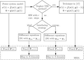
Figure 1: Procedure to obtain the matrix pencils considered.

TABLE I: Summary of matrix pencils considered. For each pencil, both the dense and sparse matrix form is given. Numerical deformation can be determined by comparing the eigenvalues of ${\boldsymbol{\rm P}}_{\scriptscriptstyle\rm PC}(z)$, ${\boldsymbol{\rm\bar{P}}}_{\scriptscriptstyle\rm PC}(z)$, $\boldsymbol{\rm P}_{d}(s)$, with those of ${\boldsymbol{P}}(s)$. To facilitate comparison, eigenvalues of $Z$-domain pencils are mapped to the $S$-domain.

Approximation by	Symbol	Sparse Matrix Form	Dense Matrix Form	Domain (Map to $S$)
N/A (DAE system)	${\boldsymbol{P}}(s)$	$s\boldsymbol{\rm E}-\boldsymbol{\rm A}$	$s\boldsymbol{\rm I}-\boldsymbol{\rm A}_{\rm s}$	$S$ (Not needed)
HM, ${\boldsymbol{y}}_{\rm int}=\boldsymbol{y}_{n}\ \$	${\boldsymbol{\rm P}}_{\scriptscriptstyle\rm PC}(z)$	$z\begin{bmatrix}\boldsymbol{\rm I}&\boldsymbol{0}\\ \boldsymbol{{g}}_{x}&\boldsymbol{{g}}_{y}\\ \end{bmatrix}-\begin{bmatrix}\boldsymbol{\rm I}+h\boldsymbol{\rm C}_{r}\boldsymbol{{f}}_{x}&h\boldsymbol{\rm C}_{r}\boldsymbol{{f}}_{y}\\ \boldsymbol{0}&\boldsymbol{\rm 0}\\ \end{bmatrix}$	$z\boldsymbol{\rm I}-(\boldsymbol{\rm I}+h\boldsymbol{\rm C}_{r}\boldsymbol{\rm A}_{\rm s})$	$Z$ ($s=\frac{{\rm log}(z)}{h}$)
HM, ${\boldsymbol{y}}_{\rm int}=\boldsymbol{y}_{n+1}\$	${\boldsymbol{\rm\bar{P}}}_{\scriptscriptstyle\rm PC}(z)$	$z\begin{bmatrix}\boldsymbol{\rm I}&-\boldsymbol{\rm B}\boldsymbol{{f}}_{y}\\ \boldsymbol{{g}}_{x}&\boldsymbol{{g}}_{y}\\ \end{bmatrix}-\begin{bmatrix}\boldsymbol{\rm I}+h\boldsymbol{\rm C}_{r}\boldsymbol{{f}}_{x}&(h\boldsymbol{\rm C}_{r}-\boldsymbol{\rm B})\boldsymbol{{f}}_{y}\\ \boldsymbol{\rm 0}&\boldsymbol{\rm 0}\\ \end{bmatrix}$	$z(\boldsymbol{\rm I}+\boldsymbol{\rm M})-(\boldsymbol{\rm I}+h\boldsymbol{\rm C}_{r}\boldsymbol{\rm A}_{\rm s}+\boldsymbol{\rm M})$	$Z$ ($s=\frac{{\rm log}(z)}{h}$)
PSA analysis in [17]	$\boldsymbol{\rm P}_{d}(s)$	$s\boldsymbol{\rm E}-\begin{bmatrix}\boldsymbol{{f}}_{x}&\boldsymbol{0}\\ \boldsymbol{{g}}_{x}&\boldsymbol{{g}}_{y}\\ \end{bmatrix}-\begin{bmatrix}\boldsymbol{0}&\boldsymbol{{f}}_{y}\\ \boldsymbol{0}&\boldsymbol{0}\\ \end{bmatrix}e^{-sh}$	$s\boldsymbol{\rm I}-\boldsymbol{{f}}_{x}+\boldsymbol{{f}}_{y}\boldsymbol{{g}}_{y}^{-1}\boldsymbol{{g}}_{x}e^{-sh}$	$S$ (Not needed)

Therefore, in terms of matrix pencils, the idea in [17] is that the numerical effect of PSA (in particular the interface error) can be seen by comparing the eigenvalues of $\boldsymbol{\rm P}_{d}(s)$ and $\boldsymbol{\rm P}(s)$. A limitation of this approach is that it does not take into account the integration scheme applied, or, equivalently, it assumes that its effect can be neglected. For example, using HM with $r=1$ or $2$ would make no difference on the interface error in view of $\boldsymbol{\rm P}_{d}(s)$. On the contrary, the matrix pencils proposed in this paper to quantify the interface error, i.e. ${\boldsymbol{\rm\bar{P}}}_{\scriptscriptstyle\rm PC}(z)$ and ${\boldsymbol{\rm P}}_{\scriptscriptstyle\rm PC}(z)$, take into account both the numerical method applied and the adopted interfacing strategy, and, from this viewpoint, they are exact.

Finally, a summary of the pencils $\boldsymbol{\rm P}(s)$, ${\boldsymbol{\rm P}}_{\scriptscriptstyle\rm PC}(z)$, ${\boldsymbol{\rm\bar{P}}}_{\scriptscriptstyle\rm PC}(z)$, and $\boldsymbol{\rm P}_{d}(s)$, is given in Table I. Moreover, a flow chart that outlines the process to derive these pencils is presented in Fig. 1. A comparison of the information given by these pencils is provided in the case study presented in Section V.

V Case Studies

In this section, we illustrate the proposed technique to study the numerical stability and accuracy of PSA. The results in Section V-A are based on the IEEE 39-bus benchmark system, whereas Section V-B is based on a 1479-bus model of the All-Island Irish Transmission System (AIITS). Simulations are carried out using the power system analysis software tool Dome [31]. The examined systems permit efficient calculation of their whole spectra, and thus, throughout this section, eigenvalues are computed with LAPACK [32], using dense matrix forms (see Table I).

V-A IEEE 39-bus system

This section considers the IEEE 39-bus system, the static and dynamic data of which are detailed in [33]. The 39-bus system comprises 10 synchronous machines represented by fourth order, two-axis models, 34 transmission lines, 12 transformers, and 19 loads. Each machine is equipped with an Automatic Voltage Regulator (AVR), a Turbine Governor (TG), and a Power System Stabilizer (PSS). The DAE model has in total 129 states and 262 algebraic variables. An equilibrium of the DAEs is obtained from the solution of the power flow problem and the initialization of dynamic components. Then, the small-signal dynamics of the system are determined by computing the eigenvalues of the matrix pencil $\boldsymbol{\rm P}(s)$ (see Section IV-A). In particular, eigenvalue analysis of $\boldsymbol{\rm P}(s)$ shows that the test system is stable around the examined equilibrium. The system’s fastest and slowest dynamics are represented, respectively, by the eigenvalues $-106.01$ and $-0.02$, which gives from (26) a stiffness ratio of $5.3\cdot 10^{3}$.

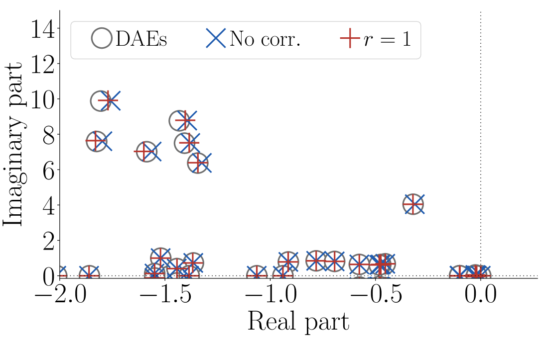
(a) $h=0.001$ s.

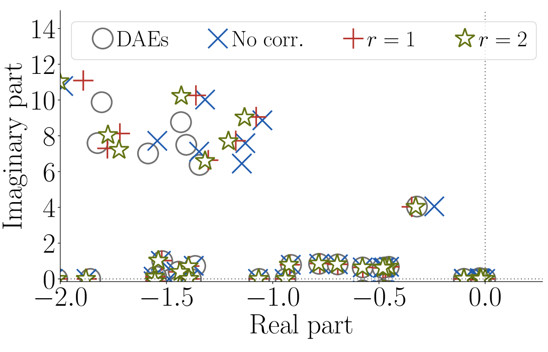
(b) $h=0.01$ s.

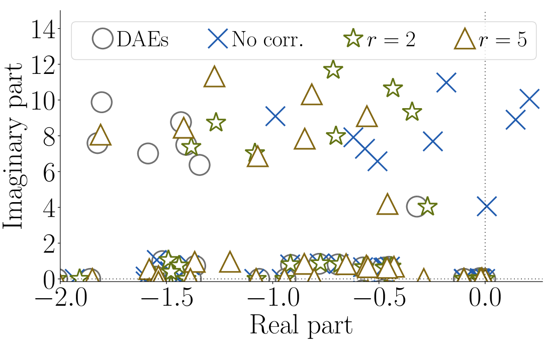
(c) $h=0.04$ s.

Figure 2: 39-bus system: Eigenvalue analysis of HM, interfacing by extrapolation.

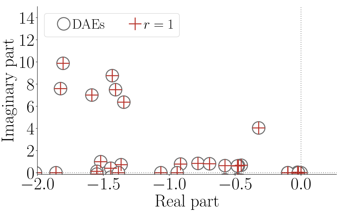
(a) $h=0.001$ s.

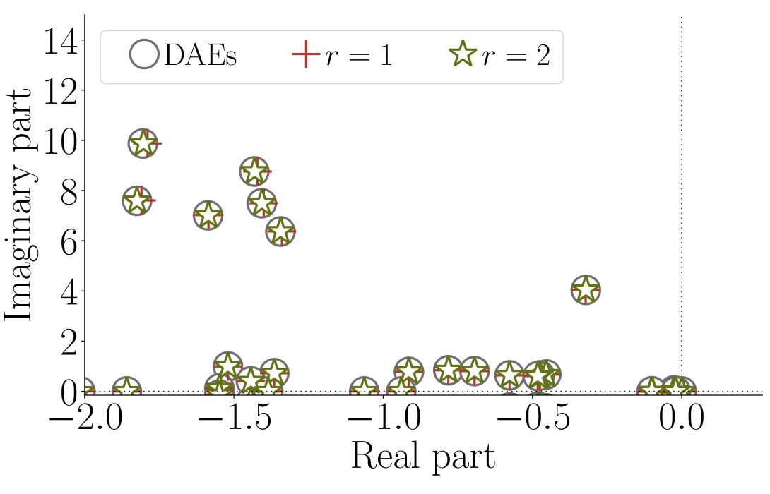
(b) $h=0.01$ s.

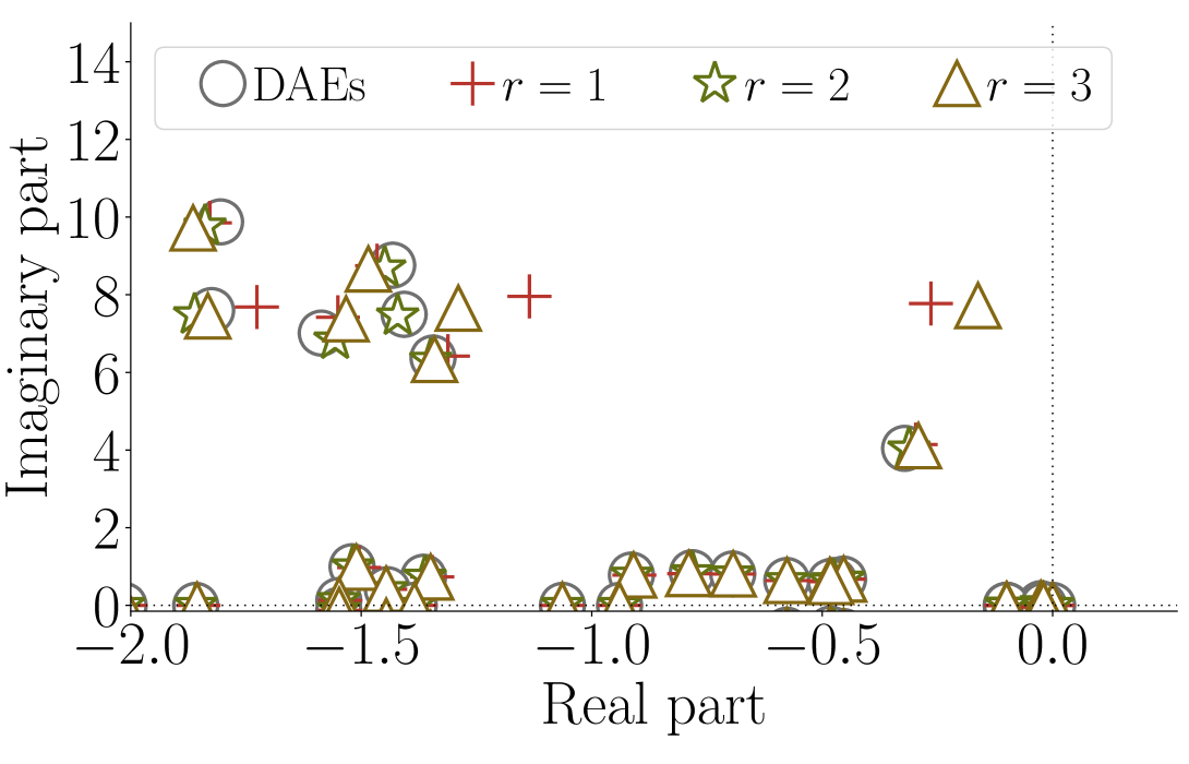
(c) $h=0.04$ s.

Figure 3: 39-bus system: Eigenvalue analysis of HM, perfect interfacing.

V-A1 Interfacing by Extrapolation

In the following, we consider that PSA is employed for the numerical integration of the system. In particular, we consider that the system is numerically solved using HM, and that interfacing is handled through extrapolation of the known values of the algebraic variables, i.e. ${\boldsymbol{y}}_{\rm int}=\boldsymbol{y}_{n}$, as described in Section III. To quantify the deformation caused to the dynamic modes of the system due to the application of the PSA-HM numerical scheme, we calculate the pencil ${\boldsymbol{\rm P}}_{\scriptscriptstyle\rm PC}(z)$ given by (38) and compute its eigenvalues, which we then map from the $Z$-domain to the $S$-domain according to (36). Figure 2 shows the numerical deformation introduced to the rightmost eigenvalues of the system for different time step sizes and for different number of corrector steps. For the sake of comparison, the case where no corrector step is applied is also provided in each plot. Note that in this case the integration scheme reduces to FEM, see (28). Results suggest that if a small time step is employed, then a single corrector step ($r=1$) suffices to refine accuracy, see Fig. 2(a), where $h=0.001$ s. For $h=0.01$ s, one corrector step is not adequate to achieve precise representation of the system’s response, while using $r=2$ slightly improves the accuracy for most modes, yet leaving a non-negligible error. Moreover, higher values of $r$ increase the computational burden of the numerical method, without however providing a proportionate improvement in precision. This is to be expected for large-enough time steps, where the effect of the extrapolation of algebraic variables becomes significant. Finally, for $h=0.04$ s, the solution is guaranteed to diverge if no corrector step is applied, since this case shows distorted eigenvalues in the right half of the $S$-plane, indicating numerical instability. In particular, the numerical stability margin of the system when no corrector is applied is found to be $h=0.035$ s. Including corrector steps, although it prevents numerical instability, does not yield a precise approximation of the system’s dynamic modes. Furthermore, interestingly, there also exist modes for which the accuracy deteriorates with higher values of $r$.

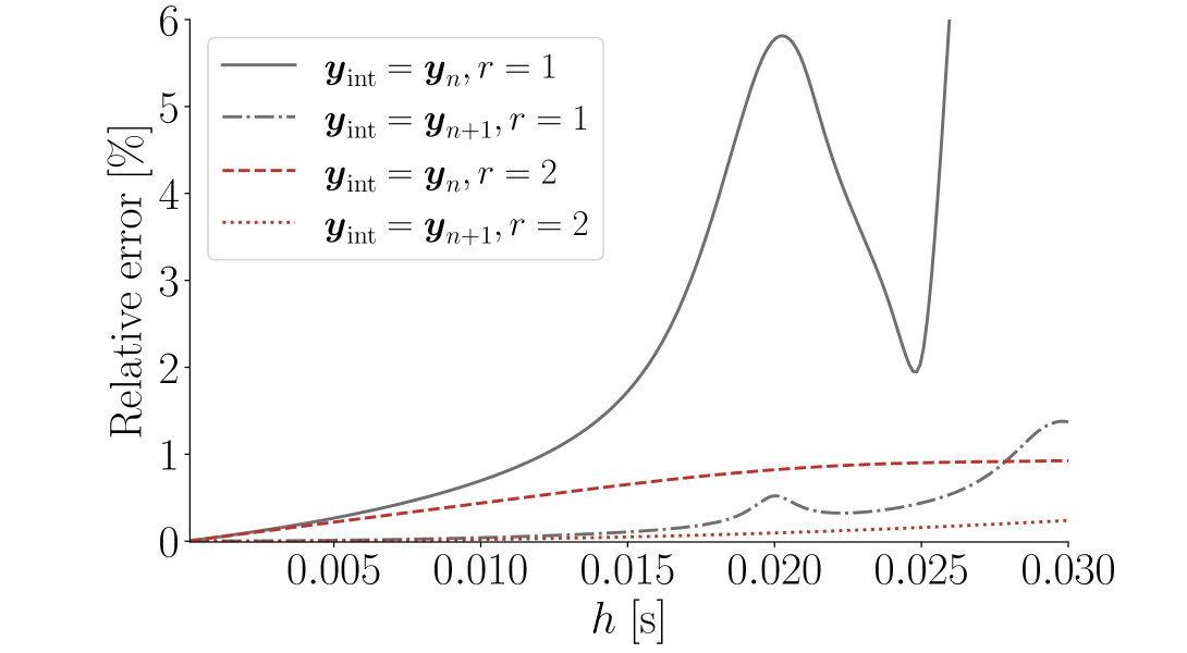
(a) Mode 1.

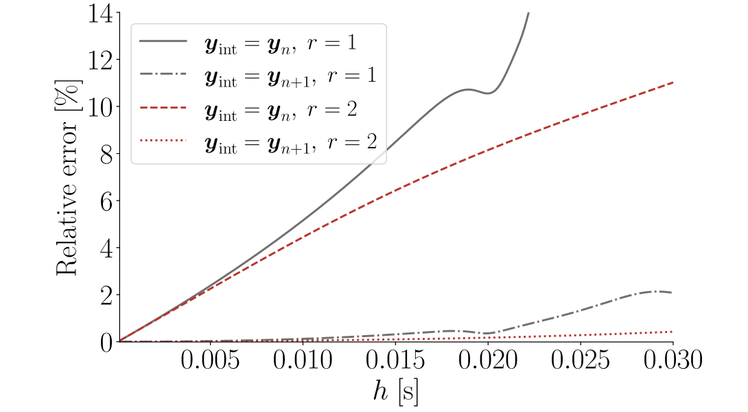
(b) Mode 2.

Figure 4: 9-bus system: Numerical deformation of least damped modes by HM.

V-A2 Comparison with Perfect Interfacing

In this section, we assume that the employed PSA-HM scheme achieves elimination of the interface error or, equivalently, that ${\boldsymbol{y}}_{\rm int}=\boldsymbol{y}_{n+1}$. The numerical deformation of the dynamic modes in this scenario can be quantified through the eigenvalues of the pencil ${\boldsymbol{\rm\bar{P}}}_{\scriptscriptstyle\rm PC}(z)$. The results for different time steps and number of corrector steps are presented in Fig. 3. These results indicate that, for time steps in the range $0.001$-$0.01$ s, using 1 to 2 corrector steps is adequate to achieve a precise approximation of the examined system’s dynamics (Figs. 3(a), 3(b)). For larger step sizes (see Fig. 3(c)), corrector steps allow only partial accuracy refinement.

In the following, we provide a further comparison of the results obtained with ${\boldsymbol{y}}_{\rm int}=\boldsymbol{y}_{n}$ and ${\boldsymbol{y}}_{\rm int}=\boldsymbol{y}_{n+1}$. With this aim, we focus on the two most critical modes of the system as defined by their damping ratios. The most lightly damped mode (hereafter Mode 1) of the system is represented by the complex pair $-0.3212\pm\jmath 4.0435$, which has damping ratio $7.92$% and natural frequency $0.64$ Hz. The second most lightly damped mode (hereafter Mode 2) is represented by the pair $-1.4318\pm\jmath 8.7610$, which has damping ratio $16.13$% and natural frequency $1.41$ Hz.

TABLE II: 39-bus system: Upper time step bounds that satisfy a $0.1$% relative error requirement for Modes 1 and 2.

$r$	1	1	2	2
$\boldsymbol{y}_{\rm int}$	$\boldsymbol{y}_{n}$	$\boldsymbol{y}_{n+1}$	$\boldsymbol{y}_{n}$	$\boldsymbol{y}_{n+1}$
max. time step [s]	0.0002	0.009	0.0002	0.015

We track the numerical deformation of Modes 1 and 2 as functions of the integration time step $h$. The results for two different setups of the HM ($r=1$ and $2$) are summarized in Fig. 4, where the relative error is defined as $100\cdot{|\hat{s}_{i}-s_{i}|}/{|s_{i}|}$, with $s_{i}$ being an eigenvalue of the system and $\hat{s}_{i}$ the corresponding numerically deformed eigenvalue. Figure 4(a) shows that, although extrapolating algebraic variables from the previous time step (${\boldsymbol{y}}_{\rm int}=\boldsymbol{y}_{n}$) introduces distortion, the structure of the integration method plays the most important role in the approximation of Mode 1. In particular, when $r=1$, the interface error causes a deformation that becomes significant for large values of $h$. Yet, with two corrector steps ($r=2$), the error is drastically reduced for all values of $h$ considered, with the relative deformation being below $1$%, regardless of the adopted interfacing strategy. On the other hand, Fig. 4(b) indicates that the interfacing strategy plays the most important role in the approximation of Mode 2. Specifically, extrapolation of algebraic variables significantly deforms Mode 2 both for small and larger time steps, with additional corrector steps not being able to notably reduce the error. Finally, assuming for the two modes a prescribed relative error requirement smaller than $0.1$%, the estimated maximum admissible time step for the four different PSA setups examined are extracted from Fig. 4 and summarized in Table II. We note here that the above discussion is based on two modes for the sake of illustration, but this is not a limitation of the proposed analysis, which can be extended to include more, or even all system modes.

V-A3 Comparison with Method in [17]

We finally provide a discussion on the accuracy of the delay-based analysis of the PSA described in [17]. As mentioned in Section IV-E, [17] focuses on the effect of extrapolating the algebraic variables while, on the other hand, effectively neglecting the impact of the specific integration method applied. To illustrate how this technique compares to the approach described in this paper, we calculate the matrix pencil $\boldsymbol{\rm P}_{d}(s)$ and compute its eigenvalues as the simulation time step $h$ is varied. Figure 5 presents the root loci obtained for the two least damped modes of the system (Modes 1 and 2). From the figure, it is obvious that the method in [17] is not able to capture modes whose deformation is more due to the integration method applied and less due to the extrapolation of algebraic variables, such as Mode 1 (see Fig. 5(a)). On the contrary, it can be accurate in tracking the approximation of modes like Mode 2, the deformation of which is mostly due to interfacing by extrapolation.

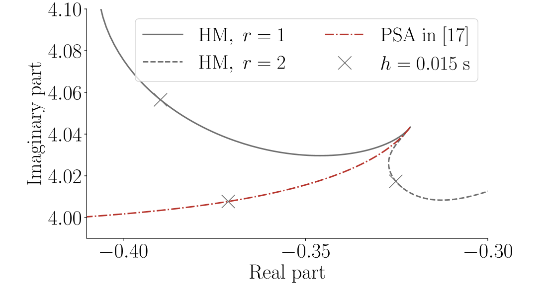
(a) Mode 1.

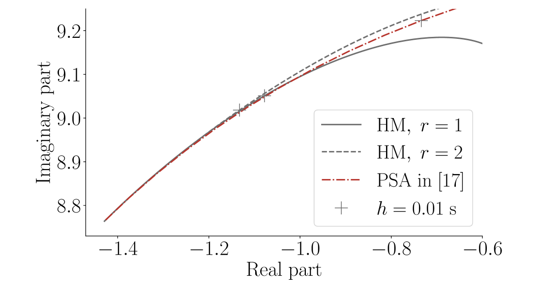
(b) Mode 2.

Figure 5: 39-bus system: HM (${\boldsymbol{y}}_{\rm int}=\boldsymbol{y}_{n}$) vs method in [17].

V-B All-Island Irish Transmission System

This section is based on a 1479-bus model of the AIITS. Topology and steady-state data have been provided by the Irish transmission system operator, EirGrid Group, whereas dynamic data have been determined based on our knowledge about the current technology of generators and automatic controllers. The system model consists of 796 lines, 1055 transformers, 245 loads, 176 wind generators, and 22 Synchronous Generators equipped with AVRs and TGs. Moreover, $6$ SGs are equipped with PSSs. In total, the system model includes 1615 state and 7225 algebraic variables. Eigenvalue analysis of the matrix pencil $\boldsymbol{\rm P}(s)$ shows that the DAE power system model is stable under small disturbances. The fastest and slowest eigenvalues of the system are respectively, $-99900.01$ and $-0.0013$. These yield a stiffness ratio of $7.6\cdot 10^{7}$. Note that this is four orders of magnitude larger than the stiffness of the 39-bus system considered in Section V-A.

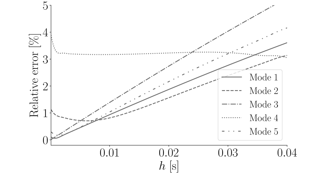
(a) Relative error.

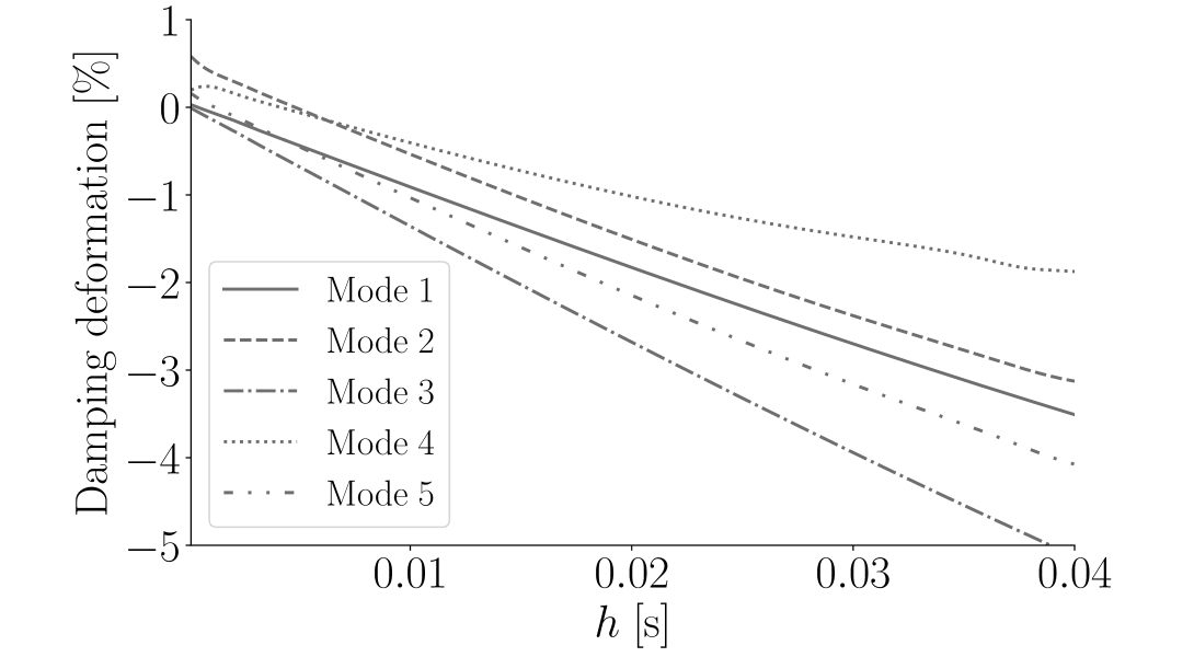
(b) Damping ratio deformation.

Figure 6: AIITS: Deformation of least damped modes by HM (${\boldsymbol{y}}_{\rm int}=\boldsymbol{y}_{n}$).

For the sake of illustration, we assume that HM with interfacing by extrapolation of algebraic variables (${\boldsymbol{y}}_{\rm int}=\boldsymbol{y}_{n}$) is employed for the solution of the AIITS. In this case, to apply the proposed technique we compute the eigenvalues of the associated pencil ${\boldsymbol{\rm P}}_{\scriptscriptstyle\rm PC}(z)$ (see (38)). The full spectrum of ${\boldsymbol{\rm P}}_{\scriptscriptstyle\rm PC}(z)$ for a given time step is computed with LAPACK in $\sim 2.4$ s. We track the deformation of the five least damped dynamic modes of the system as the integration time step size is varied and we present the results in Figs. 6.

The damping deformation shown in Fig. 6(b) is defined as follows. If $s_{i}$ is an eigenvalue of the DAE system with damping ratio $\zeta$, and $\hat{s}_{i}$ is the corresponding deformed eigenvalue with damping ratio $\hat{\zeta}$, then the damping deformation is calculated as $100\cdot(\hat{\zeta}-\zeta)$. Results indicate that numerical errors tend to increase with the time step, although they can also remain constant or decrease for some modes and in certain regions, e.g. see Modes 2 and 4 in Fig. 6 Furthermore, we note that errors for some modes can be very large even for very small time steps (an effect that was not observed on the IEEE 39-bus system). For example, the relative error of Mode 4 for $h=10^{-4}$ s is about $4$%. This effect is caused by the one-step mismatch between state and algebraic variables present when interfacing by extrapolation. This effect is further illustrated in Fig. 7.

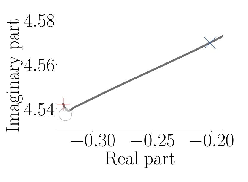
(a) Mode 1 (${\boldsymbol{y}}_{\rm int}=\boldsymbol{y}_{n}$).

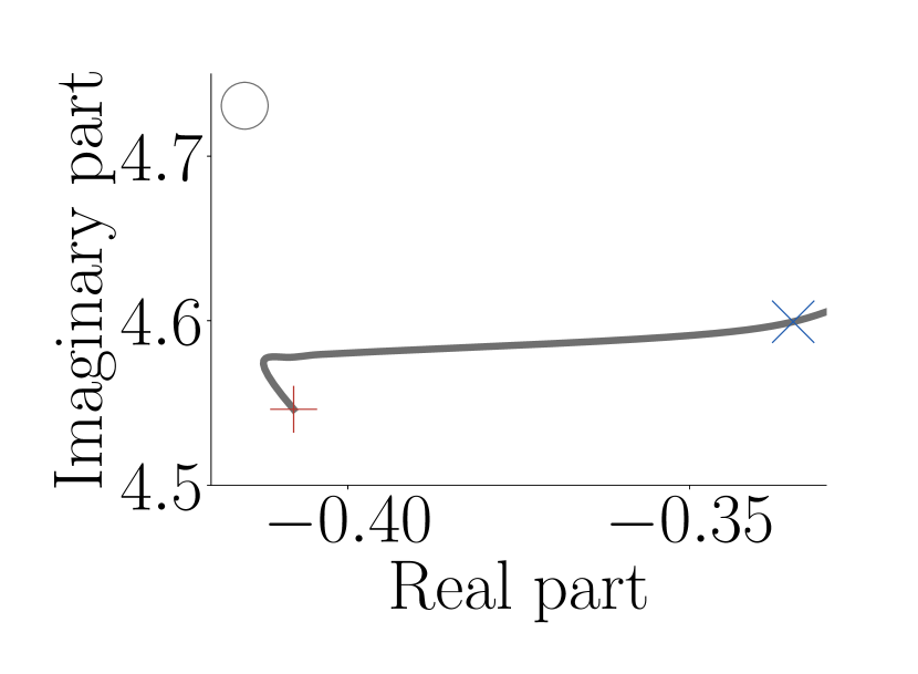
(b) Mode 4 (${\boldsymbol{y}}_{\rm int}=\boldsymbol{y}_{n}$).

Figure 7: AIITS: Eigenvalue tracking for Modes 1 and 4.

VI Conclusion

This paper proposes a novel technique based on SSSA to study the numerical stability and precision of the PSA applied for the solution of DAE power system models. The proposed technique takes into account the dynamics of the model to be solved, the integration method applied, as well as the adopted interfacing strategy, and allows estimating useful time step bounds that achieve prescribed simulation accuracy criteria. Formulation and simulation results are given for the well-known HM, while the applicability of the proposed approach to any method of the Adams-Bashforth family is duly discussed. Comparison with existing literature is also provided.

We will dedicate future work to study the effect on the proposed tool of automatic time step size and order control techniques. Moreover, we will employ the proposed approach to study the numerical robustness of state-of-art power converter models solved with PSA, such as the ones in [15, 16].

-A Proof of (33)

Let first rewrite (29) and (30) as follows:

$$\tilde{\boldsymbol{\xi}}^{(0)}_{n+1} =(\boldsymbol{\rm I}+h\boldsymbol{{f}}_{x})\tilde{\boldsymbol{x}}_{n}+h\boldsymbol{{f}}_{y}\tilde{\boldsymbol{y}}_{n}\,,$$ (46)

$$\tilde{\boldsymbol{\xi}}^{(i)}_{n+1} =(\boldsymbol{\rm I}+\frac{h}{2}\boldsymbol{{f}}_{x})\tilde{\boldsymbol{x}}_{n}+\frac{h}{2}\boldsymbol{{f}}_{x}\tilde{\boldsymbol{\xi}}^{(i-1)}_{n+1}+\frac{h}{2}\boldsymbol{{f}}_{y}(\tilde{\boldsymbol{y}}_{n}+\tilde{\boldsymbol{y}}_{\rm int})\,.$$ (47)

For the $1$-st corrector step, using (46) in (47) for $i=1$ gives:

$$\tilde{\boldsymbol{\xi}}^{(1)}_{n+1}= (\boldsymbol{\rm I}+h\boldsymbol{{f}}_{x}+\frac{h^{2}}{2}\boldsymbol{{f}}_{x}^{2})\tilde{\boldsymbol{x}}_{n}$$ (48)

$$+(\boldsymbol{\rm I}+h\boldsymbol{{f}}_{x})\frac{h}{2}\boldsymbol{{f}}_{y}\tilde{\boldsymbol{y}}_{n}+\frac{h}{2}\boldsymbol{{f}}_{y}\tilde{\boldsymbol{y}}_{\rm int}\,.$$

Similarly, for $i=2$, using (48) in (47) gives:

$$\tilde{\boldsymbol{\xi}}^{(2)}_{n+1}= (\boldsymbol{\rm I}+(\boldsymbol{\rm I}+\frac{h}{2}\boldsymbol{{f}}_{x}+\frac{h^{2}}{4}\boldsymbol{{f}}_{x}^{2})h\boldsymbol{{f}}_{x})\tilde{\boldsymbol{x}}_{n}+(\frac{1}{2}\boldsymbol{\rm I}+\frac{h}{4}\boldsymbol{{f}}_{x}$$

$$+\frac{h^{2}}{4}\boldsymbol{{f}}_{x}^{2}){h}\boldsymbol{{f}}_{y}\tilde{\boldsymbol{y}}_{n}+(\frac{1}{2}\boldsymbol{\rm I}+\frac{h}{4}\boldsymbol{{f}}_{x}){h}\boldsymbol{{f}}_{y}\tilde{\boldsymbol{y}}_{\rm int}\,.$$

By induction, we get for the $r$-th corrector step:

$$\tilde{\boldsymbol{\xi}}^{(r)}_{n+1}=(\boldsymbol{\rm I}+h\boldsymbol{\rm C}_{r}\boldsymbol{{f}}_{x})\tilde{\boldsymbol{x}}_{n} +(\boldsymbol{\rm C}_{r}-0.5\boldsymbol{\rm C}_{r-1})h\boldsymbol{{f}}_{y}\tilde{\boldsymbol{y}}_{n}$$ (49)

$$+0.5{h}\boldsymbol{\rm C}_{r-1}\boldsymbol{{f}}_{y}\tilde{\boldsymbol{y}}_{\rm int}\,,$$

where $\boldsymbol{\rm C}_{r}$ is given by (34), and $\boldsymbol{\rm C}_{r}=\boldsymbol{\rm I}+0.5h\boldsymbol{\rm C}_{r-1}\boldsymbol{{f}}_{x}$. From (31), (32), (49), we arrive at (33).

-B Proof of (41)

Let us first rewrite the predictor in the following form:

$$\boldsymbol{\xi}^{(0)}_{n+1} =\boldsymbol{x}_{n}+h\sum_{j=0}^{k-1}c_{j}\boldsymbol{f}(\boldsymbol{x}_{n-k+j+1},\boldsymbol{y}_{n-k+j+1})\,,$$ (50)

where the coefficients $c_{j}$ can be obtained by using backward difference properties, i.e.:

$$\nabla^{j+1}\boldsymbol{f}(\boldsymbol{x}_{n},\boldsymbol{y}_{n}) =\nabla^{j}\boldsymbol{f}(\boldsymbol{x}_{n},\boldsymbol{y}_{n})-\nabla^{j}\boldsymbol{f}(\boldsymbol{x}_{n-1},\boldsymbol{y}_{n-1})\,,$$

$$\nabla^{0}\boldsymbol{f}(\boldsymbol{x}_{n},\boldsymbol{y}_{n}) =\boldsymbol{f}(\boldsymbol{x}_{n},\boldsymbol{y}_{n})\,.$$

Additionally, the equilibrium point $(\boldsymbol{x}_{o},\boldsymbol{y}_{o})$ is also a fixed point of the numerical method, under the assumption that the system has been in steady-state for a time equal to $kh$. Linearizing (40) around this point, we have for the predictor:

$$\tilde{\boldsymbol{\xi}}^{(0)}_{n+1}=\tilde{\boldsymbol{x}}_{n}+h\sum_{j=0}^{k-1}c_{j}(\boldsymbol{{f}}_{x}\tilde{\boldsymbol{x}}_{n-k+j+1}+\boldsymbol{{f}}_{y}\tilde{\boldsymbol{y}}_{n-k+j+1})\,,$$ (51)

and for the $i$-th corrector step:

$$\tilde{\boldsymbol{\xi}}^{(i)}_{n+1}=\tilde{\boldsymbol{x}}_{n} +h\sum_{j=0}^{k-1}b_{j}(\boldsymbol{{f}}_{x}\tilde{\boldsymbol{x}}_{n-k+j+1}+\boldsymbol{{f}}_{y}\tilde{\boldsymbol{y}}_{n-k+j+1})$$

$$+hb_{k}(\boldsymbol{{f}}_{x}\tilde{\boldsymbol{\xi}}^{(i-1)}_{n+1}+\boldsymbol{{f}}_{y}\tilde{\boldsymbol{y}}_{\rm int})\,.$$ (52)

We proceed as follows: For $i=1$, substitution of (51) in (52) allows eliminating $\tilde{\boldsymbol{\xi}}^{(0)}_{n+1}$ and obtain $\tilde{\boldsymbol{\xi}}^{(1)}_{n+1}$. Subsequently, $\tilde{\boldsymbol{\xi}}^{(1)}_{n+1}$ is substituted in (52), and so on $\forall i<r$, until we obtain $\tilde{\boldsymbol{\xi}}^{(r)}_{n+1}$. Taking into account (31), we obtain the following form:

$$\tilde{\boldsymbol{x}}_{n+1} =\boldsymbol{\rm R}_{1}\tilde{\boldsymbol{x}}_{n}+\boldsymbol{\rm Q}_{1}\tilde{\boldsymbol{y}}_{n}+\boldsymbol{\rm R}_{2}\tilde{\boldsymbol{x}}_{n-1}+\boldsymbol{\rm Q}_{2}\tilde{\boldsymbol{y}}_{n-1}$$ (53)

$$+\ldots+\boldsymbol{\rm R}_{k}\tilde{\boldsymbol{x}}_{n-k+1}+\boldsymbol{\rm Q}_{k}\tilde{\boldsymbol{y}}_{n-k+1}\,,$$

where $\boldsymbol{\rm R}_{j}$, $\boldsymbol{\rm Q}_{j}$ are proper coefficient matrices. Considering (32) and using the notation $\mbox{$\boldsymbol{\rm x}$}_{n}=(\tilde{\boldsymbol{x}}_{n},\tilde{\boldsymbol{y}}_{n})$, (53), (32) give:

$$\boldsymbol{\rm K}\mbox{$\boldsymbol{\rm x}$}_{n+1}=\boldsymbol{\rm H}_{1}\mbox{$\boldsymbol{\rm x}$}_{n}+\boldsymbol{\rm H}_{2}\mbox{$\boldsymbol{\rm x}$}_{n-1}+\ldots+\boldsymbol{\rm H}_{k}\mbox{$\boldsymbol{\rm x}$}_{n-k+1}\,,$$ (54)

$${\text{where}}\hskip 11.38109pt\boldsymbol{\rm K}=\begin{bmatrix}\boldsymbol{\rm I}&\boldsymbol{\rm 0}\\ \boldsymbol{{g}}_{x}&\boldsymbol{{g}}_{y}\\ \end{bmatrix},\ \boldsymbol{\rm H}_{j}=\begin{bmatrix}\boldsymbol{\rm R}_{j}&\boldsymbol{\rm Q}_{j}\\ \boldsymbol{0}&\boldsymbol{0}\\ \end{bmatrix},\ j\geq 1\,.$$

Then, by setting $\boldsymbol{\rm y}_{n+1}^{[0]}=\boldsymbol{\rm x}_{n+1}$, $\boldsymbol{\rm y}_{n+1}^{[1]}=\boldsymbol{\rm x}_{n}$, $\ldots$ , $\boldsymbol{\rm y}_{n+1}^{[k-1]}=\boldsymbol{\rm x}_{n-k+2}$, and $\boldsymbol{\rm y}_{n}^{[0]}=\boldsymbol{\rm x}_{n}=\boldsymbol{\rm y}_{n+1}^{[1]}$, $\boldsymbol{\rm y}_{n}^{[1]}=\boldsymbol{\rm x}_{n-1}=\boldsymbol{\rm y}_{n+1}^{[2]}$, $\boldsymbol{\rm y}_{n}^{[k-1]}=\boldsymbol{\rm x}_{n-k+1}$. Then, (54) can be equivalently written as:

$$\boldsymbol{\rm H}_{k}\boldsymbol{\rm y}_{n}^{[k-1]}=\boldsymbol{\rm K}\boldsymbol{\rm y}_{n+1}^{[0]}-\boldsymbol{\rm H}_{1}\boldsymbol{\rm y}_{n+1}^{[1]}-\boldsymbol{\rm H}_{2}\boldsymbol{\rm y}_{n+1}^{[2]}-\ldots-\boldsymbol{\rm H}_{k-1}\boldsymbol{\rm y}_{n+1}^{[k-1]}\,.$$

Collecting the relationships above in a matrix form, we arrive at (41), with $\boldsymbol{\rm y}_{n}=(\boldsymbol{\rm y}_{n}^{[0]},\boldsymbol{\rm y}_{n}^{[1]},\ldots,\boldsymbol{\rm y}_{n}^{[k-1]})$, and:

$$\boldsymbol{\mathcal{E}}=\begin{bmatrix}\boldsymbol{0}&\boldsymbol{\rm I}\\ \boldsymbol{\rm K}&-\boldsymbol{\rm H}\\ \end{bmatrix},\ \boldsymbol{\mathcal{A}}=\begin{bmatrix}\boldsymbol{\rm I}&\boldsymbol{0}\\ \boldsymbol{0}&\boldsymbol{\rm H}_{k}\\ \end{bmatrix},\ \boldsymbol{\rm H}=[\boldsymbol{\rm H}_{1}\ \boldsymbol{\rm H}_{2}\ \ldots\ \boldsymbol{\rm H}_{k-1}]\,.$$

Georgios Tzounas (M’21) received the Diploma (M.E.) in Electrical and Computer Engineering from the National Technical Univ. of Athens, Greece, in 2017, and the Ph.D. from Univ. College Dublin (UCD), Ireland, in 2021. In Jan.-Apr. 2020, he was a visiting researcher at Northeastern Univ., Boston, MA. From Oct. 2020 to May 2022, he was a Senior Researcher at UCD. He is currently a Postdoctoral Researcher at ETH Zürich, working with the Power Systems Laboratory and the NCCR Automation project. His research interests include modelling, stability analysis and control of power systems.

Gabriela Hug (SM’14) was born in Baden, Switzerland. She received the M.Sc. degree in electrical engineering and the Ph.D. degree from the Swiss Federal Institute of Technology (ETH), Zürich, Switzerland, in 2004 and 2008, respectively. After the Ph.D. degree, she worked with the Special Studies Group of Hydro One, Toronto, ON, Canada, and from 2009 to 2015, she was an Assistant Professor with Carnegie Mellon University, Pittsburgh, PA, USA. She is currently a Professor with the Power Systems Laboratory, ETH Zurich. Her research is dedicated to control and optimization of electric power systems.

References

- [1] P. Giesl and S. Hafstein, “Review on computational methods for Lyapunov functions,” Discrete & Continuous Dynamical Systems-B, vol. 20, no. 8, p. 2291, 2015.
- [2] A. Abate, D. Ahmed, M. Giacobbe, and A. Peruffo, “Formal synthesis of Lyapunov neural networks,” IEEE Control Systems Letters, vol. 5, no. 3, pp. 773–778, 2020.
- [3] J. Anderson and A. Papachristodoulou, “Advances in computational Lyapunov analysis using sum-of-squares programming,” Discrete & Continuous Dynamical Systems-B, vol. 20, no. 8, p. 2361, 2015.
- [4] J. Machowski, Z. Lubosny, J. W. Bialek, and J. R. Bumby, Power system dynamics: stability and control. John Wiley & Sons, 2020.
- [5] P. Kundur, Power System Stability and Control. New York: Mc-Grall Hill, 1994.
- [6] I. A. Hiskens, “Power system modeling for inverse problems,” IEEE Transactions on Circuits and Systems I: Regular Papers, vol. 51, no. 3, pp. 539–551, 2004.
- [7] B. Stott, “Power system dynamic response calculations,” Proceedings of the IEEE, vol. 67, no. 2, pp. 219–241, Feb. 1979.
- [8] P. Aristidou, D. Fabozzi, and T. Van Cutsem, “Dynamic simulation of large-scale power systems using a parallel Schur-complement-based decomposition method,” IEEE Transactions on Parallel and Distributed Systems, vol. 25, no. 10, pp. 2561–2570, 2013.
- [9] G. Gurrala, A. Dimitrovski, S. Pannala, S. Simunovic, and M. Starke, “Parareal in time for fast power system dynamic simulations,” IEEE Transactions on Power Systems, vol. 31, no. 3, pp. 1820–1830, 2015.
- [10] S. Jin, Z. Huang, R. Diao, D. Wu, and Y. Chen, “Comparative implementation of high performance computing for power system dynamic simulations,” IEEE Transactions on Smart Grid, vol. 8, no. 3, pp. 1387–1395, 2017.
- [11] T. Noda, K. Takenaka, and T. Inoue, “Numerical integration by the 2-stage diagonally implicit Runge-Kutta method for electromagnetic transient simulations,” IEEE Transactions on Power Delivery, vol. 24, no. 1, pp. 390–399, 2009.
- [12] C. Fu, J. D. McCalley, and J. Tong, “A numerical solver design for extended-term time-domain simulation,” IEEE Transactions on Power Systems, vol. 28, no. 4, pp. 4926–4935, 2013.
- [13] D. Fabozzi and T. Van Cutsem, “Simplified time-domain simulation of detailed long-term dynamic models,” in Proceedings of the IEEE PES General Meeting, 2009, pp. 1–8.
- [14] J. Sanchez-Gasca, R. D’Aquila, W. Price, and J. Paserba, “Variable time step, implicit integration for extended-term power system dynamic simulation,” in Proceedings of Power Industry Computer Applications Conference, 1995, pp. 183–189.
- [15] D. Ramasubramanian, W. Wang, P. Pourbeik, E. Farantatos, A. Gaikwad, S. Soni, and V. Chadliev, “Positive sequence voltage source converter mathematical model for use in low short circuit systems,” IET Generation, Transmission & Distribution, vol. 14, no. 1, pp. 87–97, 2020.
- [16] D. Ramasubramanian, X. Wang, S. Goyal, M. Dewadasa, Y. Li, R. O’Keefe, and P. Mayer, “Parameterization of generic positive sequence models to represent behavior of inverter based resources in low short circuit scenarios,” Electric Power Systems Research, vol. 213, p. 108616, 2022.
- [17] F. Milano, “Delay-based numerical stability of the partitioned-solution approach,” in Proceedings of the IEEE PES General Meeting. IEEE, 2016, pp. 1–5.
- [18] G. Tzounas, I. Dassios, and F. Milano, “Small-signal stability analysis of numerical integration methods,” IEEE Transactions on Power Systems, vol. 37, no. 6, pp. 4796–4806, Nov. 2022.
- [19] ——, “Small-signal stability analysis of implicit integration methods for power systems with time delays,” Electric Power System Research, vol. 211, no. 108266, Oct. 2022.
- [20] T. Davis, Direct methods for sparse linear systems. SIAM, 2006.
- [21] F. Milano, I. Dassios, M. Liu, and G. Tzounas, Eigenvalue Problems in Power Systems. CRC Press, Taylor & Francis Group, 2020.
- [22] I. Dassios, G. Tzounas, and F. Milano, “ The Möbius transform effect in singular systems of differential equations,” Applied Mathematics and Computation, vol. 361, pp. 338–353, 2019.
- [23] S. Tomov, J. Dongarra, and M. Baboulin, “Towards dense linear algebra for hybrid GPU accelerated manycore systems,” Parallel Computing, vol. 36, no. 5-6, pp. 232–240, 2010.
- [24] G. Tzounas, I. Dassios, M. Liu, and F. Milano, “Comparison of numerical methods and open-source libraries for eigenvalue analysis of large-scale power systems,” Applied Sciences, vol. 10, no. 21, 2020.
- [25] Y. Li, G. Geng, and Q. Jiang, “An efficient parallel Krylov-Schur method for eigen-analysis of large-scale power systems,” IEEE Transactions on Power Systems, vol. 31, no. 2, pp. 920–930, 2015.
- [26] ——, “A parallelized contour integral Rayleigh–Ritz method for computing critical eigenvalues of large-scale power systems,” IEEE Transactions on Smart Grid, vol. 9, no. 4, pp. 3573–3581, 2016.
- [27] PSS/E 33.0, Program Application Guide Volume 2. Siemens, 2011.
- [28] General Electric Energy Consulting, “General Electric (GE) PSLF,” geenergyconsulting.com/practice-area/software-products/pslf.
- [29] G. C. Verghese, I. J. Pérez-Arriaga, and F. C. Schweppe, “Selective modal analysis with applications to electric power systems, part ii: the dynamic stability problem,” IEEE Transactions on Power Apparatus and Systems, vol. PAS-101, no. 9, pp. 3126–3134, Sep. 1982.
- [30] J. H. Chow, Power System Coherency and Model Reduction, ser. Power Electronics and Power Systems 94. New York: Springer-Verlag, 2013.
- [31] F. Milano, “A Python-based software tool for power system analysis,” in Proceedings of the IEEE PES General Meeting, Jul. 2013.
- [32] E. Angerson, Z. Bai, J. Dongarra, A. Greenbaum, A. McKenney, J. D. Croz, S. Hammarling, J. Demmel, C. Bischof, and D. Sorensen, “LAPACK: A portable linear algebra library for high-performance computers,” in Proceedings of the ACM/IEEE Conference on Supercomputing, Nov. 1990, pp. 2–11.
- [33] Illinois Center for a Smarter Electric Grid (ICSEG), “IEEE 39-Bus System,” publish.illinois.edu/smartergrid/ieee-39-bus-system/.