Abstract

Modern statistical analysis often encounters high dimensional models but with limited sample sizes. This makes the target data based statistical estimation very difficult. Then how to borrow information from another large sized source data for more accurate target model estimation becomes an interesting problem. This leads to the useful idea of transfer learning. Various estimation methods in this regard have been developed recently. In this work, we study transfer learning from a different perspective. Specifically, we consider here the problem of testing for transfer learning sufficiency. By transfer learning sufficiency (denoted as the null hypothesis), we mean that, with the help of the source data, the useful information contained in the feature vectors of the target data can be sufficiently extracted for predicting the interested target response. Therefore, the rejection of the null hypothesis implies that information useful for prediction remains in the feature vectors of the target data and thus calls for further exploration. To this end, we develop a novel testing procedure and a centralized and standardized test statistic, whose asymptotic null distribution is analytically derived. Simulation studies are presented to demonstrate the finite sample performance of the proposed method. A deep learning related real data example is presented for illustration purpose.

KEYWORDS: Deep Learning; High Dimensional Data; Logistic Regression; Testing Statistical Hypothesis; Transfer Learning; Transfer Learning Sufficiency

Modern statistical analysis often encounters challenging situations, where the target model is of high dimension but the accessible sample is of a very limited size. This is particularly true for medical, genetic, and image related studies, where the supporting samples are hard to obtain due to ethical or cost issues (Li et al., 2022a). Consider for example the analysis of skin cutaneous melanoma (SKCM) disease. The widely used SKCM dataset consists of only 347 patient samples but a total of 18,335 gene expression levels measured for each sample. Consider modern deep learning researches as another example. For this research field, the topic of few-shot learning (i.e., training models on a few samples) has attracted arising attentions from researchers, because data collection and labeling is often very expensive (Wang et al., 2021). Given the fact that deep learning models often have thousands of hundreds of parameters to estimate, the problem of “small sample size and high dimensionality” becomes inevitable. Then, how to accurately train a high dimensional target model with a limited sample size becomes a practically important problem.

One seemingly very promising way to solve this problem is transfer learning (Pan and Yang, 2009). By transfer learning, we expect that there exists another huge sized auxiliary dataset, which is different from but somewhat related with the target dataset. For convenience, we refer to this auxiliary dataset as a source dataset. The probability distribution generating the source/target dataset is referred to as the source/target population. It is remarkable that the source population is often different from the target population. To fix this idea, let ($X,Y$) and ($X^{*},Y^{*}$) be the observations generated from the target population and source population, respectively. The interested response $Y$ in the target population could be totally different from $Y^{*}$ in the source population. For example, $Y^{*}$ is often assumed to be a categorical response taken values in $\{0,1,...,K\}$, but $Y$ is allowed to be continuous. Nevertheless, the covariate $X$ and $X^{*}$ must be of the same dimension $p$. Otherwise, no transfer learning can be conducted. Although the sample size of target data is often limited, the size of the source data is expected to be huge. Consequently, various high dimensional models can be estimated on the source data with reasonable accuracy. Then how to transfer the valuable information learned from the source data to the target model becomes the key issue. To this end, various transfer learning methods have been developed.

In the computer science literature, there exist a variety of strategies for transfer learning; see Weiss et al. (2016) and Farahani et al. (2020) for an excellent review. Among them, the arguably most typical transfer learning strategy is the feature-based approach (Oquab et al., 2014; Shin et al., 2016; Guo et al., 2018). The key idea is to find a common feature space underlying the source data and having predictive power for the target model in the meanwhile. Consider for example a categorical response $Y^{*}$. Then a deep learning model can often be written as $P(Y^{*}=k)=\exp\{Z_{\mathbb{B}}^{\top}(X^{*})\gamma_{k}\}/1+\sum_{k=1}^{K}\exp\{Z_{\mathbb{B}}^{\top}(X^{*})\gamma_{k}\}$, where $Z_{\mathbb{B}}(\cdot)$ is a feature generating function (Donahue et al., 2014; He et al., 2016; Ji et al., 2021). It transforms the high dimensional vector $X^{*}$ into a lower dimensional one as $Z_{\mathbb{B}}(X^{*})$ in the feature space. Since the dimension of $X^{*}$ is large, the dimension of the unknown parameter $\mathbb{B}$ for the feature generating function is also high. Fortunately, the source data size is often huge. Therefore, the unknown parameter $\mathbb{B}$ (or its linear transformation) can be estimated with reasonable accuracy. Once $\mathbb{B}$ is estimated (denoted by $\widehat{\mathbb{B}}$), the estimated feature generating function $Z_{\widehat{\mathbb{B}}}(\cdot)$ can be readily applied to the target data with the high dimensional covariate $X$. This leads to the newly estimated feature vector $Z_{\widehat{\mathbb{B}}}(X)$. By modeling the relationship between $Z_{\widehat{\mathbb{B}}}(X)$ and $Y$, the valuable information learned from the source data can be transferred to the target model.

Recently, transfer learning has attracted great attention from the statistical literature, but from a somewhat different perspective. A number of researchers have developed novel new algorithms for different models, such as linear regression (Li et al., 2022a), generalized linear regression (Tian and Feng, 2022), nonparametric regression (Cai and Wei, 2021), multiple testing (Liang et al., 2022), and Gaussian graphical models (Li et al., 2022b). The general idea here is to estimate the target model and source model simultaneously, and then utilize the similarity between the source and target models to improve the estimation accuracy of the target model. For example, Li et al. (2022a) propose a Trans-Lasso method for transfer learning in a high dimensional linear regression model. The basic idea is to pool source data and target data together so that an initial estimator can be obtained. Thereafter, the bias of the initial estimator is corrected by the target data. Similar methods are also developed for generalized linear regression models by Tian and Feng (2022).

Inspired by these pioneer researches from both the computer science literature and statistical literature, we take here a very unique perspective to study transfer learning. On one side, our approach shares similar spirit as those in the computer science literature. Specifically, we assume a feature generating function $Z_{\mathbb{B}}(X)$, which can be learned by the source data and then transferred to the target model for generating lower dimensional feature vectors. We follow this direction mainly because it is probably the most widely adopted transfer learning strategy in practice. In fact, many most commonly used deep learning frameworks (e.g., TensorFlow and Pytorch) have implemented this strategy for transfer learning. On the other side, our proposed method also benefits from those pioneered works in the statistical literature. We are inspired by the statistical theory developed therein. By these inspirational statistical theory, one can gain better understanding about the information transferring dynamics between the source data and target data. As a consequence, new estimation and inference procedure can be developed with statistical guarantees.

As our first attempt, we follow the past literature to start with the simplest but possibly the most important feature generating function, i.e., the linear transformation (Lu and Zhang, 2010; Fan and Fine, 2013). Specifically, we assume for the source data a standard multinominal logistic regression model as $P(Y^{*}=k)=\exp\{X^{*\top}\beta_{k}\}/[1+\sum_{k=1}^{K}\exp\{X^{*\top}\beta_{k}\}]$ for $1\leq k\leq K$. Then the arguably simplest feature generating function can be defined as $Z^{*}=Z_{\mathbb{B}}(X^{*})=\mathbb{B}^{\top}X^{*}$, where $\mathbb{B}=(\beta_{1},\beta_{2},...,\beta_{K})\in\mathbb{R}^{p\times K}$ with $K\ll p$. We next assume for the target data a binary logistic regression model as $P(Y=1)=\exp(X^{\top}\theta)/\{1+\exp(X^{\top}\theta)\}$, where $\theta\in\mathbb{R}^{p}$ is the target parameter of interest. We then consider how to transfer the knowledge learned from the source data about $\mathbb{B}$ to help the estimation of $\theta$. The key issue here is whether $\theta\in\mathcal{S}(\mathbb{B})$, where $\mathcal{S}(\mathbb{B})$ stands for the linear space generated by the column vectors of $\mathbb{B}$. If $\theta\in\mathcal{S}(\mathbb{B})$ indeed happens, we then should have $\theta=\mathbb{B}\gamma$ for some $\gamma\in\mathbb{R}^{K}$. Accordingly, the target model can be rewritten as $P(Y=1)=\exp(Z^{\top}\gamma)/\{1+\exp(Z^{\top}\gamma)\}$, where $Z=\mathbb{B}^{\top}X\in\mathbb{R}^{K}$. Thereafter, instead of working on the high dimensional vector $X$ directly, we can work on the dimension-reduced vector $Z$ without any loss about the prediction accuracy. In this case, we say the transfer learning is sufficient in the sense that $P(Y=1|\mathbb{B}^{\top}X)=P(Y=1|X)$. Otherwise, if $\theta\notin\mathcal{S}(\mathbb{B})$, we should have $P(Y=1|\mathbb{B}^{\top}X)\neq P(Y=1|X)$ for a significant amount of $X$. Therefore, there exists non-negligible loss in prediction accuracy. In this case, we say the transfer learning is insufficient. In other words, valuable information useful for more accurate prediction about $Y$ remains in $X$ and has not been fully captured by $\mathbb{B}^{\top}X$.

Practically, $\mathbb{B}$ is an unknown parameter. Then how to estimate $\mathbb{B}$ becomes an important problem. With the help of source data, we can easily obtain an estimate $\widehat{\mathbb{B}}=(\widehat{\beta}_{1},\widehat{\beta}_{2},...,\widehat{\beta}_{K})$, where $\widehat{\beta}_{k}$ is (for example) the maximum likelihood estimator of $\beta_{k}$ computed on the source data. Under appropriate regularity conditions, we should have $\widehat{\mathbb{B}}$ to be consistent and asymptotically normal as $N\to\infty$. Since the source data usually have a huge sample size, we can expect $\widehat{\mathbb{B}}$ to have sufficient accuracy. With the estimated $\widehat{\mathbb{B}}$, the lower dimensional vector $Z$ can be replaced by $\widehat{Z}=\widehat{\mathbb{B}}^{\top}X$. Then the target model using $\widehat{Z}$ as the input can be estimated accordingly. This leads to a maximum likelihood estimator $\widehat{\gamma}$ for the coefficient $\gamma$. With the relationship $\theta=\mathbb{B}\gamma$, an estimator for $\theta$ can be defined as $\widehat{\theta}=\widehat{\mathbb{B}}\widehat{\gamma}$, which we refer to as the transfer learning (TL) estimator. To theoretically support our method, a rigorous asymptotic theory has been developed. We find that, under appropriate regularity conditions, the resulting TL estimator $\widehat{\theta}$ can be asymptotically as efficient as the oracle estimator. Here the oracle estimator is defined to be the ideal estimator obtained with a perfectly recovered lower dimensional feature vector $Z_{\mathbb{B}}(X)$.

Since the target data are often extremely valuable, we wish the useful information contained in the target feature has been fully utilized with the help of transfer learning. Otherwise, a significant amount of valuable information remains in the target feature for further exploration. This leads to an interesting theoretical problem. That is how to test sufficiency for transfer learning. To solve the problem, we develop here a novel testing procedure. The key idea is as follows. As mentioned before, a consistent estimator for the regression coefficient $\theta$ can be obtained for the target model, under the null hypothesis of transfer learning sufficiency and with the help of the source data. Note that this task can hardly be accomplished by using the target data only. Thereafter, pseudo residuals can be differentiated. Under appropriate regularity conditions, they should be uncorrelated with every single feature asymptotically. Accordingly, we should expect the sample covariance between the pseudo residual and each predictor to be close to 0. We are then inspired to have those sample covariances computed for each predictor squared and summed up together. This leads to an interesting test statistic sharing similar spirit as that of Lan et al. (2014). However, as demonstrated by Lan et al. (2014), to make test statistic of this form have a non-degenerate asymptotic distribution, appropriate centralization operation is necessarily needed. This leads to a centralized test statistic with significantly reduced bias and variability. We show rigorously that this centralized test statistic is asymptotically distributed as a standard normal distribution under the null hypothesis and after appropriate location-scale transformation. Extensive simulation studies are presented to demonstrate this testing procedure’s finite sample performance. A deep learning related real dataset is analyzed for illustration purpose.

The rest of the article is organized as follows. Section 2 describes our theoretical framework for transfer learning. Based on the proposed theoretical framework, a transfer-learning based maximum likelihood estimator is developed for the target model. Its asymptotical properties are then rigorously studied. Thereafter, the problem of testing sufficiency for transfer learning is studied. In this regard, a high dimensional testing procedure is developed based on the sum of squared sample covariances between the pseudo-residuals and predictors. After appropriate centralization and standardization, its asymptotical null distribution is rigorously established. The finite sample performance of the proposed methodology is then evaluated by extensive numerical studies on both simulated and real datasets in Section 3. Lastly, Section 4 concludes the paper with a brief discussion.

2.1. Transfer Learning Estimator

Consider a target dataset with a total of $n$ samples. Let $(X_{i},Y_{i})$ be the observation collected from the $i$th subject ($1\leq i\leq n$) in the target dataset. Here $Y_{i}\in\{0,1\}$ is a binary response and $X_{i}=(X_{i1},\dots,X_{ip})^{\top}\in\mathbb{R}^{p}$ is the associated $p$-dimensional features. Without loss of generality, we assume all features in $X_{i}$ are centralized such that $E(X_{i})=0$. Further assume that $(X_{i},Y_{i})$ for different subjects are independently and identically distributed. To model the regression relationship between $X_{i}$ and $Y_{i}$, we consider a standard logistic regression model as

$$P\Big{(}Y_{i}=1\big{|}X_{i}\Big{)}=\frac{\exp(X_{i}^{\top}\theta)}{1+\exp(X_{i}^{\top}\theta)}=g\Big{(}X_{i}^{\top}\theta\Big{)},$$ (2.1)

where $\theta=(\theta_{1},\dots,\theta_{p})^{\top}\in\mathbb{R}^{p}$ is the $p$-dimensional regression coefficient, and $g(x)=\exp(x)/\{1+\exp(x)\}$ is the sigmoid function for any scalar $x$. We refer to (2.1) as the target model. To estimate the target model, the maximum likelihood estimation method can be used. Specifically, a log-likelihood function can be constructed as

$$\mathcal{L}_{n}^{\text{Target}}(\theta)=\sum_{i=1}^{n}\Bigg{[}Y_{i}\Big{(}X_{i}^{\top}\theta\Big{)}-\log\bigg{\{}1+\exp\Big{(}X_{i}^{\top}\theta\Big{)}\bigg{\}}\Bigg{]}.$$ (2.2)

Then the maximum likelihood estimator (MLE) of the target model can be obtained as $\widehat{\theta}_{\text{mle}}^{\text{Target}}=\mbox{argmax}_{\theta}\mathcal{L}_{n}^{\text{Target}}(\theta)$. If the feature dimension $p$ is fixed and the target sample size $n\to\infty$, we should have $\widehat{\theta}_{\text{mle}}^{\text{Target}}$ to be $\sqrt{n}$-consistent and asymptotically normal (McCullagh and Nelder, 1989; Shao, 2003). Unfortunately, we often encounter the situation, where the target sample size $n$ is very limited but the feature dimension $p$ is ultrahigh. This leads to a challenging situation with $n\approx p$ or $n<p$. In this case, the maximum likelihood estimator should be biased or even computationally infeasible (Sur and Candes, 2019; Candes and Sur, 2020).

To solve this problem, we can seek for the help of transfer learning. The general idea is to borrow information from the source data. Specifically, define $(X_{i}^{*},Y_{i}^{*})$ to be the observation collected for the $i$th sample with $1\leq i\leq N$ in the source data. Assume the covariate $X_{i}^{*}=(X_{i1}^{*},\dots,X_{ip}^{*})^{\top}\in\mathbb{R}^{p}$ to have the same dimension as $X_{i}$. Similarly, we also assume $E(X_{i}^{*})=0$. However, different from the target data, we assume the response $Y_{i}^{*}$ in the source data to be a $(K+1)$-level categorical variable, i.e., $Y_{i}^{*}\in\{0,1,\dots,K\}$. We typically expect $K$ to be relatively large so that ample amount of information can be provided by $Y_{i}^{*}$. In the meanwhile, $K$ should not be too large neither. Instead, it should be much smaller than the target sample size $n$. Otherwise, the rich information provided by $Y_{i}^{*}$ cannot be conveniently transferred to the target model with a limited sample size.

To study the regression relationship between $X_{i}^{*}$ and $Y_{i}^{*}$, we assume the following multi-class logistic regression model as

$$P(Y_{i}^{*}=k|X_{i}^{*})=\frac{\exp(X_{i}^{*\top}\beta_{k})}{1+\sum_{j=1}^{K}\exp(X_{i}^{*\top}\beta_{j})}\text{ for }1\leq k\leq K,$$ (2.3)

where $\beta_{k}=(\beta_{k1},\dots,\beta_{kp})^{\top}\in\mathbb{R}^{p}$ is the $p$-dimension regression coefficient for class $k$ with respect to the base class $0$. We refer to (2.3) as the source model, and define $\mathbb{B}=(\beta_{1},\dots,\beta_{K})\in\mathbb{R}^{p\times K}$ to be the corresponding coefficient matrix. Then the log-likelihood function of the source model can be spelled out as

$$\mathcal{L}^{\text{Source}}_{N}(\mathbb{B})=\sum_{i=1}^{N}\Bigg{[}\sum_{k=1}^{K}I(Y_{i}^{*}=k)X_{i}^{*\top}\beta_{k}-\log\bigg{\{}1+\sum_{k=1}^{K}\exp\Big{(}X_{i}^{*\top}\beta_{k}\Big{)}\bigg{\}}\Bigg{]}.$$

Thereafter, the maximum likelihood estimator of the source model can be computed as $\widehat{\mathbb{B}}^{\text{Source}}_{\text{mle}}=(\widehat{\beta}_{1},\dots,\widehat{\beta}_{K})=\mbox{argmax}_{\mathbb{B}}\mathcal{L}^{\text{Source}}_{N}(\mathbb{B})$. Under appropriate regularity conditions, we should have $\widehat{\mathbb{B}}^{\text{Source}}_{\text{mle}}$ to be consistent and asymptotically normal as $N\to\infty$ (Fan and Peng, 2004). It is remarkable that, we assume in this work the source sample size $N$ is much larger than both the target sample size $n$ and the feature dimension $p$. Therefore, based on the large source data, the parameter $\mathbb{B}$ can be estimated with sufficient accuracy. Next, we consider how to estimate the parameter $\theta$ for the target model by transferring useful information from $\widehat{\mathbb{B}}^{\text{Source}}_{\text{mle}}$.

To borrow information from the source data by $\widehat{\mathbb{B}}^{\text{Source}}_{\text{mle}}$, we need to define a feature generating function $Z_{\mathbb{B}}(X)$, which can be learned by the source data and then transferred to the target data. Given the source model (2.3), we can define an arguably simplest feature generating function as $Z^{*}_{i}=Z_{\mathbb{B}}(X^{*}_{i})=\mathbb{B}^{\top}X^{*}_{i}\in\mathbb{R}^{K}$ for the source data. We typically assume $K\ll p$, so that the dimension of the new feature $Z^{*}_{i}$ generated by the feature generating function is much smaller than that of the original feature $X^{*}_{i}$. Then the question is whether this feature generating function $Z_{\mathbb{B}}(X)$ is applicable for the target data. In other words, whether the rich information contained in the original high dimensional feature $X_{i}$ in the target data can be sufficiently represented by the dimension-reduced feature $Z_{i}=Z_{\mathbb{B}}(X_{i})=\mathbb{B}^{\top}X_{i}\in\mathbb{R}^{K}$. If the answer is positive, we should be able to write $X_{i}^{\top}\theta=Z_{\mathbb{B}}^{\top}(X_{i})\gamma=(X_{i}^{\top}\mathbb{B})\gamma=Z_{i}^{\top}\gamma$ for some $\gamma=(\gamma_{1},\dots,\gamma_{K})^{\top}\in\mathbb{R}^{K}$. Accordingly, we should have $\theta=\mathbb{B}\gamma$. If this happens, we should have $P(Y_{i}=1|X_{i})=P(Y_{i}=1|Z_{i})$. Therefore, we say the transfer learning offered by $Z_{\mathbb{B}}(X)$ is sufficient. Otherwise, we say the transfer learning is insufficient.

Recall that the dimension of $Z_{i}$ is much smaller than the dimension of $X_{i}$. Therefore, instead of working on the high dimensional vector $X_{i}$ directly, we can work on the dimension-reduced vector $Z_{i}$ with the regression coefficient $\gamma$. Then the target model (2.1) can be rewritten as

$$P\Big{(}Y_{i}=1\big{|}Z_{i}\Big{)}=\frac{\exp(Z_{i}^{\top}\gamma)}{1+\exp(Z_{i}^{\top}\gamma)}.$$

Since $\mathbb{B}$ is an unknown parameter, we have to replace it by some appropriate estimator. As discussed before, one natural choice is the maximum likelihood estimator $\widehat{\mathbb{B}}_{\text{mle}}^{\text{Source}}$. Accordingly, we can replace $Z_{i}$ by $\widehat{Z}_{i}=\widehat{\mathbb{B}}_{\text{mle}}^{\text{Source}\top}X_{i}$. This leads to the following working model as

$$P\Big{(}Y_{i}=1\big{|}Z_{i}\Big{)}\approx\frac{\exp(\widehat{Z}_{i}^{\top}\gamma)}{1+\exp(\widehat{Z}_{i}^{\top}\gamma)}.$$

Accordingly, a working log-likelihood function can be written as

$$\mathcal{L}_{n}(\gamma;\widehat{Z})=\sum_{i=1}^{n}\Bigg{[}Y_{i}\Big{(}\widehat{Z}_{i}^{\top}\gamma\Big{)}-\log\bigg{\{}1+\exp\Big{(}\widehat{Z}_{i}^{\top}\gamma\Big{)}\bigg{\}}\Bigg{]}.$$ (2.4)

Then a maximum likelihood type estimator for $\gamma$ can be obtained by maximizing (2.4) as $\widehat{\gamma}=\mbox{argmax}_{\gamma}{\mathcal{L}}_{n}(\gamma;\widehat{Z})$. Recall that $\theta=\mathbb{B}\gamma$. Then an estimator for $\theta$ can be defined as $\widehat{\theta}^{\text{Transfer}}=\widehat{\mathbb{B}}_{\text{mle}}^{\text{Source}}\widehat{\gamma}$, which utilizes the information not only learned from the target data but also transferred from the source data. For convenience, we refer to it as a transfer learning (TL) estimator.

2.2. The Transferred Maximum Likelihood Estimator

We next study the asymptotic properties of the TL estimator. Let $\lambda_{\min}(A)$ and $\lambda_{\max}(A)$ be the smallest and largest eigenvalues of an arbitrary square matrix $A$, respectively. Define $\pi_{ik}=P(Y_{i}^{*}=k|X_{i}^{*})$ and $\pi_{i}=(\pi_{i1},\dots,\pi_{iK})^{\top}\in\mathbb{R}^{K}$. Write $W_{i}=\mbox{diag}(\pi_{i})-\pi_{i}\pi_{i}^{\top}$. Define $\dot{\mathcal{L}}_{n}(\gamma;Z)\in\mathbb{R}^{K}$ to be the first-order derivative of the oracle log-likelihood function $\mathcal{L}_{n}(\gamma;Z)$ with respect to $\gamma$. Here the oracle log-likelihood function $\mathcal{L}_{n}(\gamma;Z)$ is computed based on the true feature vector $Z_{i}$ instead of its estimated counterpart $\widehat{Z}_{i}$. Further define $I(\gamma)=n^{-1}E\big{[}\dot{\mathcal{L}}_{n}(\gamma;Z)\dot{\mathcal{L}}_{n}(\gamma;Z)^{\top}\big{]}=E\big{[}g(Z_{i}^{\top}\gamma)\{1-g(Z_{i}^{\top}\gamma)\}Z_{i}Z_{i}^{\top}\big{]}$ as the Fisher information matrix of the oracle log-likelihood function. Next, we define the sub-Gaussian norm for a random variable $U$ as $\|U\|_{\psi_{2}}=\inf\{t>0:E\exp(U^{2}/t^{2})\leq 2\}$, and for a random vector $V$ as $\|V\|_{\psi_{2}}=\sup_{\|u\|=1}\|u^{\top}V\|_{\psi_{2}}$. Then we say a random vector $V$ is sub-Gaussian if $\|V\|_{\psi_{2}}<\infty$; see Vershynin (2018) for more detailed discussions about the sub-Gaussian norm. For an arbitrary matrix $A=(a_{ij})\in\mathbb{R}^{m\times n}$, define its Frobenius norm as $\|A\|_{F}=\sqrt{\sum_{i=1}^{m}\sum_{j=1}^{n}a_{ij}^{2}}$. To study the theoretical properties of the TL estimator, the following technical conditions are necessarily needed:

• As $N\to\infty$, we should have $n^{2}\log N/N\to 0$ and $p\to\infty$. Moreover, there exists a positive constant $0<C<\infty$ such that $p\leq Cn$.

• Both the random vectors $X_{i}^{*}$ and $X_{i}$ are sub-Gaussian.

• Denote $\otimes$ to be the kronecker product. As $p\to\infty$, there exist two positive constants $0<C_{\min}\leq C_{\max}<\infty$ such that: (1) $C_{\min}\leq\lambda_{\min}\{E(X_{i}^{*}X_{i}^{*\top})\}\leq\lambda_{\max}\{E(X_{i}^{*}X_{i}^{*\top})\}\leq C_{\max}$, (2) $C_{\min}\leq\lambda_{\min}[E\{W_{i}\otimes(X_{i}^{*}X_{i}^{*\top})\}]\leq\lambda_{\max}[E\{W_{i}\otimes(X_{i}^{*}X_{i}^{*\top})\}]\leq C_{\max}$, (3) $C_{\min}\leq\lambda_{\min}\{E(X_{i}X_{i}^{\top})\}\leq\lambda_{\max}\{E(X_{i}X_{i}^{\top})\}\leq C_{\max}$, and (4) $C_{\min}\leq\lambda_{\min}(\Sigma_{\gamma})\leq\lambda_{\max}(\Sigma_{\gamma})\leq C_{\max}$. Here $\Sigma_{\gamma}=E(\varepsilon_{i}^{2}X_{i}X_{i}^{\top})$, where $\varepsilon_{i}=Y_{i}-E(Y_{i}|X_{i})$ is the pseudo residual.

• As $p\to\infty$, there exists a positive constant $\tau_{\max}>0$ such that $E\|Z_{i}\|^{4}\leq\tau_{\max}$ and $E(X_{i}^{\top}X_{j})^{4}\leq\tau_{\max}p^{2}$ for any $i\neq j$.

• As $p\to\infty$, we have $\lambda_{\max}(\mathbb{B}^{\top}\mathbb{B})\leq\tau_{\max}$, where $\tau_{\max}$ is the same as in (C4).

Condition (C1) implies that, the sample size of the source data should be sufficiently large in the sense that $n^{2}\log N/N\to 0$. Condition (C1) also restricts the divergence rate of the feature dimension $p$ such that it should not be of higher order than the target sample size $n$. However, we allow $p>n$. In that case, we should have $C>1$. Condition (C2) is slightly stronger than a standard moment condition. It is trivially satisfied if $X_{i}$ follows a multivariate normal distribution. A similar but stronger condition as $\sup_{i}\|X_{i}\|=O_{p}(\sqrt{p})$ has been used in the past literature (Portnoy, 1985; Welsh, 1989; He and Shao, 2000; Wang, 2011). Condition (C3) imposes uniform bounds on the maximum and minimum eigenvalues of various positive definite matrices with diverging dimension $p$. Condition (C4) imposes two moment conditions about $Z_{i}$ and $X_{i}$, which are fairly reasonable. To fix the idea, consider for example a special case with $X_{i}$ following a multivariate standard normal distribution. Then it can be verified that $E(X_{i}^{\top}X_{j})^{4}=3\mbox{tr}^{2}\{E(X_{i}X_{i}^{\top})\}+6\mbox{tr}\{E^{4}(X_{i}X_{i}^{\top})\}=3p^{2}+6p\leq\tau_{\max}p^{2}$ with $\tau_{\max}=9$. Condition (C5) is also a fairly reasonable assumption. To gain some quick understanding about this condition, assume Condition (C5) is violated. Then there should exist a vector $\gamma$ with unit length $||\gamma||=1$. In the meanwhile, we have $\gamma^{\top}(\mathbb{B}^{\top}\mathbb{B})\gamma=\lambda_{\max}(\mathbb{B}^{\top}\mathbb{B})\to\infty$ as $p\to\infty$. Then we have $\mbox{var}(Z_{i}^{\top}\gamma)=\mbox{var}(X_{i}^{\top}\mathbb{B}\gamma)=\gamma^{\top}\mathbb{B}^{\top}E(X_{i}X_{i}^{\top})\mathbb{B}\gamma\geq C_{\min}\{\gamma^{\top}(\mathbb{B}^{\top}\mathbb{B})\gamma\}=C_{\min}\lambda_{\max}(\mathbb{B}^{\top}\mathbb{B})\to\infty$. In this case, the information contained in $Z_{i}$ as measured by $\mbox{var}(Z_{i}^{\top}\gamma)$ diverges to infinity. Thus we can make nearly perfect prediction for $Y_{i}$ by $Z_{i}$. This is obviously not reasonable. Therefore, we must have Condition (C5) hold. With the above conditions, we then have the following theorem.

Theorem 1.

Assume the conditions (C1)-(C5), then $\|\widehat{\mathbb{B}}_{\text{mle}}^{\text{Source}}-\mathbb{B}\|_{F}=O_{p}(\sqrt{p/N})$.

The technical proof of Theorem 1 is similar to that of Fan and Peng (2004). However, for the sake of theoretical completeness, we provide the detailed proof in Appendix A. By Theorem 1, we know the maximum likelihood estimator $\widehat{\mathbb{B}}_{\text{mle}}^{\text{Source}}$ of the source model is $\sqrt{N/p}$-consistent. It implies that, with a huge source sample size, the parameter $\mathbb{B}$ can be estimated with reasonable accuracy. Once $\widehat{\mathbb{B}}_{\text{mle}}^{\text{Source}}$ is computed, a lower-dimensional feature vector can be computed as $\widehat{Z}_{i}=\widehat{\mathbb{B}}_{\text{mle}}^{\text{Source}\top}X_{i}$. Then a revised target model with $\widehat{Z}_{i}$ as the input can be established. The theoretical properties of the corresponding estimator $\widehat{\gamma}$ are summarized in the following theorem.

Theorem 2.

Assume the conditions (C1)-(C5), then we have: (1) $\sqrt{n}(\widehat{\gamma}-\gamma)\stackrel{{\scriptstyle d}}{{\to}}N(0,I(\gamma)^{-1})$; (2) $\sqrt{n}v^{\top}\Big{(}\widehat{\theta}^{\text{Transfer}}-\theta\Big{)}/\sigma(v)\stackrel{{\scriptstyle d}}{{\to}}N(0,1)$, where $v$ is an arbitrary $p$-dimensional vector in $\mathcal{S}(\mathbb{B})$ with unit length, and $\sigma^{2}(v)=v^{\top}\mathbb{B}I(\gamma)^{-1}\mathbb{B}^{\top}v$.

The proof of Theorem 2 can be found in Appendix B. Theorem 2 suggests that, with the help of the source model estimator $\widehat{\mathbb{B}}_{\text{mle}}^{\text{Source}}$, the estimator $\widehat{\gamma}$ of the target model should be $\sqrt{n}$-consistent and asymptotically normal. In particular, its asymptotic distribution remains to be the same as that of the oracle estimator, which is defined as $\widehat{\gamma}_{\text{oracle}}=\mbox{argmax}_{\gamma}{\mathcal{L}}_{n}(\gamma;Z)$. This is the maximum likelihood estimator obtained with the true low dimensional feature vector $Z_{i}$ instead of its estimator $\widehat{Z}_{i}$. Furthermore, with the relationship $\theta=\mathbb{B}\gamma$, the TL estimator of $\theta$ can be obtained as $\widehat{\theta}^{\text{Transfer}}=\widehat{\mathbb{B}}_{\text{mle}}^{\text{Source}}\widehat{\gamma}$. Then Theorem 2 suggests that, for any $v\in\mathcal{S}(\mathbb{B})$, the estimator $v^{\top}\widehat{\theta}^{\text{Transfer}}$ is $\sqrt{n}$-consistent for $v^{\top}\theta$ and asymptotically normal.

2.3. Testing Sufficiency for Transfer Learning

The nice theoretical properties obtained in the previous section hinge on one critical assumption. That is, all information contained in $X_{i}$ about $Y_{i}$ in the target data can be sufficiently represented by $Z_{i}=\mathbb{B}^{\top}X_{i}$. In other words, the transfer learning is sufficient. However, for a practical dataset, whether the transfer learning is sufficient is not immediately clear. Thus there is great need to develop a principled statistical procedure to test for the transfer learning sufficiency. We are then motivated to develop in this section a novel solution in this regard.

Our method is motivated by the following interesting observation. If the transfer learning is sufficient in the sense that all information contained in $X_{i}$ about $Y_{i}$ has been sufficiently captured by $Z_{i}$, we should have $E(Y_{i}|Z_{i},X_{i})=E(Y_{i}|Z_{i})=g(Z_{i}^{\top}\gamma)$. Then the pseudo residual $\varepsilon_{i}=Y_{i}-E(Y_{i}|Z_{i},X_{i})=Y_{i}-g(Z_{i}^{\top}\gamma)$ should be uncorrelated with the feature vector $X_{i}$ in the sense that $E(\varepsilon_{i}X_{i})=0$. Practically, the true feature vector $Z_{i}$ and the coefficient parameter $\gamma$ are both unknown. However, with the help of source data, they can be both estimated as $\widehat{Z}_{i}=\widehat{\mathbb{B}}_{\text{mle}}^{\text{Source}\top}X_{i}$ and $\widehat{\gamma}=\mbox{argmax}_{\gamma}{\mathcal{L}}_{n}(\gamma;\widehat{Z})$. Then the estimated pseudo residual can be obtained as $\widehat{\varepsilon}_{i}=Y_{i}-g(\widehat{Z}_{i}^{\top}\widehat{\gamma})$. We then should reasonably expect $n^{-1}\sum_{i=1}^{n}\widehat{\varepsilon}_{i}X_{i}\approx 0$. This leads to a preliminary test statistic as $T_{1}=\|n^{-1}\sum_{i=1}^{n}\widehat{\varepsilon}_{i}X_{i}\|^{2}=n^{-2}\widehat{\varepsilon}^{\top}\mathbb{X}\mathbb{X}^{\top}\widehat{\varepsilon}$, where $\widehat{\varepsilon}=(\widehat{\varepsilon}_{1},\dots,\widehat{\varepsilon}_{n})^{\top}\in\mathbb{R}^{n}$ is the estimated pseudo residual vector and $\mathbb{X}=(X_{1},\dots,X_{n})^{\top}\in\mathbb{R}^{n\times p}$ is the design matrix. If the null hypothesis of transfer learning sufficiency is incorrect, we should expect $\widehat{\varepsilon}_{i}$ to be materially correlated with $X_{ij}$ for some $1\leq j\leq p$. This should make the value of $T_{1}$ unreasonably large. Similar test statistics were also constructed by Lan et al. (2014) but for testing statistical significance of a high dimensional regression model. To understand the asymptotic behavior of $T_{1}$, it is important to compute its mean and variance under the null hypothesis of transfer learning sufficiency. This leads to the following theorem.

Theorem 3.

Assume the conditions (C1)-(C4) and the null hypothesis of transfer learning sufficiency. Define $\Sigma_{\gamma}=E(\varepsilon_{i}^{2}X_{i}X_{i}^{\top})=E[g(Z_{i}^{\top}\gamma)\{1-g(Z_{i}^{\top}\gamma)\}X_{i}X_{i}^{\top}]$. We further assume that $n^{2}p/N\to 0$. Then we have $T_{1}=T^{*}_{1}+o_{p}(\sqrt{p}/n)$, where $T_{1}^{*}=n^{-2}\varepsilon^{\top}\mathbb{X}\mathbb{X}^{\top}\varepsilon$ and $\varepsilon=(\varepsilon_{1},\dots,\varepsilon_{n})^{\top}\in\mathbb{R}^{n}$ is the true pseudo residual vector. For $T^{*}_{1}$, we have $E(T^{*}_{1})=n^{-1}\mbox{tr}(\Sigma_{\gamma})$ and $\mbox{var}(T^{*}_{1})=n^{-3}\mbox{var}(\varepsilon_{i}^{2}X_{i}^{\top}X_{i})+2n^{-2}(1-n^{-1})\mbox{tr}(\Sigma_{\gamma}^{2})$.

The proof of Theorem 3 can be found in Appendix C. By Theorem 3 and Condition (C3), we have $E(T_{1}^{*})\geq(2n)^{-1}\mbox{tr}(\Sigma_{\gamma})\geq 0.5C_{\min}n^{-1}p$. Further define $\text{SE}(T_{1}^{*})=\{\mbox{var}(T_{1}^{*})\}^{1/2}$. Then by Theorem 3 and Condition (C3), we can obtain $\text{SE}(T_{1}^{*})\leq\big{\{}4n^{-3}E(X_{i}X_{i}^{\top})^{4}+4n^{-2}(1-n^{-1})\mbox{tr}(\Sigma_{\gamma}^{2})\big{\}}^{1/2}\leq 2c_{\max}(n^{-3/2}p+n^{-1}p^{1/2})$, where $c_{\max}=\max\{C_{\max},\tau_{\max}\}$. Therefore, we should have $E(T_{1}^{*})/\text{SE}(T_{1}^{*})\to\infty$ as $n\to\infty$. Consequently, it is impossible for the random variable $T_{1}/\text{SE}(T_{1})$ to converge in distribution to any non-degenerated probability distribution. Similar interesting phenomenon was also obtained in Lan et al. (2014). To solve this problem, applying appropriate centralization on $T_{1}$ is needed.

2.4. A Centralized Test Statistic

As discussed above, the order of $E(T_{1})$ is considerably larger than that of $\text{SE}(T_{1})$. Therefore, appropriate centralization on $T_{1}$ is inevitably needed. Similar operations have been used in the past literature (Li and Racine, 2007; Lan et al., 2014). Note that the leading term of $E(T_{1})$ is linearly related to $tr(\Sigma_{\gamma})$ where $\Sigma_{\gamma}=E(\varepsilon_{i}^{2}X_{i}X_{i}^{\top})$. Therefore, the bias of $T_{1}$ can be significantly reduced by subtracting this term, as long as an accurate estimator for $\Sigma_{\gamma}$ can be obtained. In this regard, a simple moment estimator of $\Sigma_{\gamma}$ can be constructed as $\widehat{\Sigma}_{\gamma}=n^{-1}\sum_{i=1}^{n}\widehat{\varepsilon}_{i}^{2}X_{i}X_{i}^{\top}$. This leads to a centralized test statistic as $T_{2}=T_{1}-n^{-1}\mbox{tr}(\widehat{\Sigma}_{\gamma})$. The mean and variance of $T_{2}$ are then given by the following theorem.

Theorem 4.

Assume the conditions (C1)-(C4) and the null hypothesis of transfer learning sufficiency. Further assume $n^{2}p/N\to 0$. Then we have $T_{2}=T_{2}^{*}+o_{p}(\sqrt{p}/n)$, where $T_{2}^{*}=n^{-2}\varepsilon^{\top}(\mathbb{X}\mathbb{X}^{\top}-\mathbb{D}_{X})\varepsilon$ and $\mathbb{D}_{X}=\mbox{diag}\{X_{1}^{\top}X_{1},\dots,X_{n}^{\top}X_{n}\}\in\mathbb{R}^{n\times n}$. For $T_{2}^{*}$, we have $E(T_{2}^{*})=0$ and $\mbox{var}(T_{2}^{*})=2n^{-2}\mbox{tr}(\Sigma_{\gamma}^{2})\{1+o(1)\}$.

The detailed proof of Theorem 4 can be found in Appendix D. By Theorem 4, we obtain the following interesting findings. First, we find that the asymptotical variance of the centralized statistic $T_{2}^{*}$ is significantly smaller than that of $T_{1}^{*}$, by an amount of $n^{-3}\mbox{var}(\varepsilon_{i}^{2}X_{i}^{\top}X_{i})=O_{p}(p^{2}/n^{3})$. Second, note that $\text{SE}(T_{2}^{*})=\{\mbox{var}(T_{2}^{*})\}^{1/2}=\{2n^{-2}\mbox{tr}(\Sigma_{\gamma}^{2})\}^{1/2}\geq C_{\min}n^{-1}p^{1/2}$. Compared with the order of $\text{SE}(T_{2}^{*})$, we find the order of $E(T_{2}^{*})$ is a small order term. Therefore a formal standardized test statistic can be constructed as $T_{3}=T_{2}/\sqrt{2n^{-2}\mbox{tr}(\Sigma_{\gamma}^{2})}$, whose asymptotic behavior is summarized in the following theorem.

Theorem 5.

Assume the conditions (C1)-(C4) and the null hypothesis of transfer learning sufficiency. Further assume $n^{2}p/N\to 0$, then $T_{3}\stackrel{{\scriptstyle d}}{{\to}}N(0,1)$ as $N\to\infty$.

The detailed proof of Theorem 5 can be found in Appendix E. Theorem 5 suggests that, the centralized and standardized test statistic $T_{3}$ is asymptotically distributed as a standard normal distribution. Note that the term $\mbox{tr}(\Sigma_{\gamma}^{2})$ is involved in $T_{3}$. Therefore, to practically apply this test procedure, a ratio consistent estimator for $\mbox{tr}(\Sigma_{\gamma}^{2})$ is needed. To solve this problem, one natural idea is to use the plug-in estimator $\mbox{tr}(\widehat{\Sigma}_{\gamma}^{2})$. The expectation of this plug-in estimator can be calculated as $E\big{\{}\mbox{tr}(\widehat{\Sigma}_{\gamma}^{2})\big{\}}=n^{-1}E\big{\{}\varepsilon_{i}^{4}(X_{i}^{\top}X_{i})^{2}\}+(1-n^{-1})\mbox{tr}(\Sigma_{\gamma}^{2})\{1+o(1)\big{\}}$. By Condition (C3), we can derive $n^{-1}E\big{\{}\varepsilon_{i}^{4}(X_{i}^{\top}X_{i})^{2}\big{\}}\geq(2n)^{-1}\big{\{}E(\varepsilon_{i}^{2}X_{i}^{\top}X_{i})\big{\}}^{2}=(2n)^{-1}\mbox{tr}^{2}(\Sigma_{\gamma})\geq C_{\min}^{2}(2n)^{-1}p^{2}$. We can also have $\mbox{tr}(\Sigma_{\gamma}^{2})\leq C_{\max}^{2}p$. This suggests that $E\{\mbox{tr}(\widehat{\Sigma}_{\gamma}^{2})\}/\mbox{tr}(\Sigma_{\gamma}^{2})\geq p/n$. As a result, when $p$ is larger than $n$, $\mbox{tr}(\widehat{\Sigma}_{\gamma}^{2})$ cannot be ratio consistent for $\mbox{tr}(\Sigma_{\gamma}^{2})$ in the sense that $\mbox{tr}(\widehat{\Sigma}_{\gamma}^{2})/\mbox{tr}(\Sigma_{\gamma}^{2})\stackrel{{\scriptstyle p}}{{\nrightarrow}}1$ as $N{\to}\infty$. The inconsistency of $\mbox{tr}(\widehat{\Sigma}_{\gamma}^{2})$ is mainly due to the extra bias term $n^{-1}E\big{\{}\varepsilon_{i}^{4}(X_{i}^{\top}X_{i})^{2}\big{\}}$. Therefore, we are motivated to construct a bias corrected estimator for $\mbox{tr}(\Sigma_{\gamma}^{2})$ as

$$\widehat{\mbox{tr}(\Sigma_{\gamma}^{2})}=\mbox{tr}(\widehat{\Sigma}_{\gamma}^{2})-n^{-2}\sum_{i=1}^{n}\widehat{\varepsilon}_{i}^{4}\big{(}X_{i}^{\top}X_{i}\big{)}^{2}=n^{-2}\sum_{i\neq j}\widehat{\varepsilon}_{i}^{2}\widehat{\varepsilon}_{j}^{2}\big{(}X_{i}^{\top}X_{j}\big{)}^{2}.$$

The ratio consistency property of $\widehat{\mbox{tr}(\Sigma_{\gamma}^{2})}$ is summarized by the following theorem.

Theorem 6.

Assume the conditions (C1)-(C4) and the null hypothesis of transfer learning sufficiency. Further assume $n^{2}p/N\to 0$, then $\widehat{\mbox{tr}(\Sigma_{\gamma}^{2})}/\mbox{tr}(\Sigma_{\gamma}^{2})\stackrel{{\scriptstyle p}}{{\to}}1$ as $N{\to}\infty$.

The detailed proof of Theorem 6 can be found in Appendix F. Theorem 6 implies that $\widehat{\mbox{tr}(\Sigma_{\gamma}^{2})}$ is a ratio consistent estimator for $\mbox{tr}(\Sigma_{\gamma}^{2})$ as $N{\to}\infty$. With this ratio consistent estimator, we can construct a practically computable test statistic as ${T}_{4}=T_{2}/\{2n^{-2}\widehat{\mbox{tr}}(\Sigma_{\gamma}^{2})\}^{1/2}$. Under the null hypothesis of transfer learning sufficiency, we should have $T_{4}$ to follow a standard normal distribution asymptotically. Then the null hypothesis of transfer learning sufficiency should be rejected, if the value of $T_{4}$ is sufficiently large. Specifically, we should reject the null hypothesis at a given significance level $\alpha$ if ${T}_{4}>z_{1-\alpha}$, where $z_{\alpha}$ is the $\alpha$th quantile of the standard normal distribution. Otherwise, the null hypothesis of transfer learning sufficiency should be accepted.

3.1. Simulation Setups

To demonstrate the finite sample performance of the TL estimator and the test statistic for transfer learning sufficiency, we present here a number of simulation studies. The whole study contains two parts. The first part focuses on the estimation performance of the TL estimator $\widehat{\theta}^{\text{Transfer}}$. The objective is to numerically investigate the influence of feature dimension $p$, target sample size $n$, and the source sample size $N$ on the statistical efficiency of the TL estimator under the null hypothesis of transfer learning sufficiency. The second part investigates the finite sample performance of the proposed test statistic $T_{4}$ for transfer learning sufficiency. Both the size (i.e., the Type I error) and the power are evaluated under different experimental settings of $(p,n,N)$. For the entire study, we fix the class number $K=8$ in the source data. Then with a given feature dimension $p$, target sample size $n$, and source sample size $N$, the detailed data generation procedure is present as follows.

Source Data. We first generate the covariate $X_{i}^{*}\in\mathbb{R}^{p}$ with $1\leq i\leq N$ independently and identically from a multivariate normal distribution with mean 0 and covariance matrix $\Sigma=(\sigma_{j_{1}j_{2}})_{p\times p}$ with $\sigma_{j_{1}j_{2}}=0.5^{|j_{1}-j_{2}|}$. Then we generate a random vector $\tilde{\beta}_{k}\in\mathbb{R}^{p}$ for $0\leq k\leq K$. All the elements of $\tilde{\beta}_{k}$ are independently and identically generated from a standard normal distribution. Next we define $\beta_{k}=\tilde{\beta}_{k}/\|\tilde{\beta}_{k}\|-\tilde{\beta}_{0}/\|\tilde{\beta}_{0}\|$. Thereafter the source response $Y_{i}^{*}$ is generated according to $P(Y_{i}^{*}=k|X_{i}^{*})=\exp(X_{i}^{*\top}\beta_{k})/\big{\{}1+\sum_{j=1}^{K}\exp(X_{i}^{*\top}\beta_{j})\big{\}}$ for $1\leq k\leq K$. Accordingly, we have $P(Y_{i}^{*}=0|X_{i}^{*})=1/\big{\{}1+\sum_{j=1}^{K}\exp(X_{i}^{*\top}\beta_{j})\big{\}}$. Let $\mathbb{B}=(\beta_{1},\dots,\beta_{k})\in\mathbb{R}^{p\times K}$. We then have a feature generating function as $Z_{\mathbb{B}}(X_{i}^{*})=\mathbb{B}^{\top}X_{i}^{*}$.

Target Data. We first generate the target covariate $X_{i}\in\mathbb{R}^{p}$ with $1\leq i\leq n$ independently and identically from the same multivariate normal distribution as for the source data. Next we compute the low dimensional feature vector $Z_{i}=Z_{\mathbb{B}}(X_{i})=\mathbb{B}^{\top}X_{i}\in\mathbb{R}^{K}$ for the target data. Then we consider how to generate the response $Y_{i}$. Specifically, under the null hypothesis of transfer learning sufficiency, we generate $Y_{i}$ according to $P(Y_{i}=1|X_{i})=P(Y_{i}=1|Z_{i})=\exp(Z_{i}^{\top}\gamma)/\{1+\exp(Z_{i}^{\top}\gamma)\}$ with $\gamma=(0.5,0.5,0.5,0.5,0.5,-1.25,0,0)^{\top}\in\mathbb{R}^{K}$. Therefore, the true coefficient $\theta$ associated with $X_{i}$ in the target mode is given by $\theta=\mathbb{B}\gamma$. In contrast, if the transfer learning is insufficient, we then generate $Y_{i}$ as $P(Y_{i}=1|X_{i})=\exp(Z_{i}^{\top}\gamma+X_{i1}\delta)/\{1+\exp(Z_{i}^{\top}\gamma+X_{i1}\delta)\}$, where $\delta>0$ is a fixed constant.

3.2. Results of Estimation Performance

We investigate the finite sample performance of the proposed TL estimator under the null hypothesis of transfer learning sufficiency. We start with the case $p<n$. In this case, we compare three different estimators of $\theta$. They are, respectively: (1) our proposed TL estimator $\widehat{\theta}^{\text{Transfer}}$; (2) the oracle estimator $\widehat{\theta}^{\text{Oracle}}$, which is also a transfer learning estimator but using the true coefficient matrix $\mathbb{B}$ instead of its estimated counterpart $\widehat{\mathbb{B}}_{\text{mle}}^{\text{Source}}$; and (3) the target data based maximum likelihood estimator $\widehat{\theta}_{\text{mle}}^{\text{Target}}$ according to (2.2). Let the feature dimension $p\in(40,80,120)$, the target sample size $n\in(400,600,800)$, and the source sample size $N\in(20000,40000,80000)$. Then different combinations of $(p,n,N)$ are studied. For each $(p,n,N)$ combination, we generate the target data and source data according to the generation process as described in Section 3.1. The experiment is randomly replicated for a total of $B=1,000$ times. For the $b$-th replication, denote one particular estimator of $\theta$ as $\widehat{\theta}^{(b)}$. Then we evaluate its estimation performance by mean squared error (MSE) as $\text{MSE}_{(b)}=p^{-1}\sum_{j=1}^{p}(\widehat{\theta}^{(b)}_{j}-\theta_{j})^{2}$. This leads to a total of $B=1,000$ MSE values. They are then log-transformed and boxplotted in Figure 1.

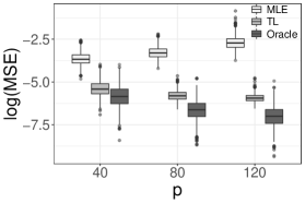
(a) $n=600$ and $N=40000$

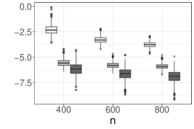
(b) $p=80$ and $N=40000$

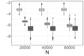
(c) $p=80$ and $n=600$

Figure 1: Boxplots of log-transformed MSE of the maximum likelihood estimator (MLE), our proposed transfer learning (TL) estimator, and the oracle transfer learning estimator in the $p<n$ case. Different combinations of $(p,n,N)$ are considered to explore the influence of $(p,n,N)$ on the estimation performance of the three estimators.

By Figure 1, we can draw the following conclusions. First, for all cases, the log(MSE) values of the MLE are always larger than those of our proposed TL estimator and the oracle estimator. This is expected, because the MLE is obtained by directly estimating a high dimensional model without any help from the source data. As a consequence, its performance is worse than the two transfer learning estimators. Second, with the feature dimension $p$ and source sample size $N$ fixed, the log(MSE) values of the TL estimator, along with the other estimators, decrease as the target sample size $n$ increases. These results demonstrate the consistency of the TL estimator, which is in line with Theorem 2. Last, with the feature dimension $p$ and target sample size $n$ fixed, we find the log(MSE) values of the TL estimator become closer to those of the oracle estimator as $N\to\infty$. This result also corroborates our theoretical findings in Theorem 2. That is, when the source sample size is large enough, the TL estimator can perform as well as the oracle estimator asymptotically.

Next consider the case with $n\leq p<N$. In this case, the MLE $\widehat{\theta}_{\text{mle}}^{\text{Target}}$ is not computable. Therefore, we only compare the estimation performance of our proposed TL estimator $\widehat{\theta}^{\text{Transfer}}$ with the oracle estimator $\widehat{\theta}^{\text{Oracle}}$. We consider the feature dimension $p\in(100,200,300)$, the target sample size $n\in(75,100,150)$, and the source sample size $N\in(20000,40000,80000)$. Then different combinations of $(p,n,N)$ are studied; see Figure 2 for details. For each combination, we randomly replicate the experiment for a total of $B=1,000$ times. For each experiment, the two transfer learning estimators are computed and the MSE values are calculated to evaluate the estimation performance. This leads to $B=1,000$ MSE values for each estimator, which are then log-transformed and boxplotted in Figure 2. Similar with the case $p<n$, we find the log(MSE) values of the two estimators both decrease as the target sample size $n$ increases, implying the consistency the two estimators. In addition, the two estimators become closer to each other as $N\to\infty$. This finding suggests that, once we provide the source data with a sufficiently large sample size, the high dimensionality effect on the estimation performance of $\theta$ is very limited.

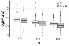
(a) $n=100$ and $N=40000$

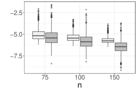
(b) $p=300$ and $N=40000$

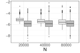
(c) $p=300$ and $n=100$

Figure 2: Boxplots of log-transformed estimation error of our proposed transfer learning (TL) estimator and the oracle transfer learning estimator in the $n\leq p<N$ case. Different combinations of $(p,n,N)$ are considered to explore the influence of $(p,n,N)$ on the estimation performance of the two estimators.

3.3. Results of Testing Performance

In this section, we investigate the finite sample performance of the proposed testing procedure for transfer learning sufficiency. We first evaluate the size of the testing procedure. In this regard, we should generate the target data under the null hypothesis of transfer learning sufficiency. Specifically, we generate $Y_{i}$ according to $P(Y_{i}=1|X_{i})=P(Y_{i}=1|Z_{i})=\exp(Z_{i}^{\top}\gamma)/\{1+\exp(Z_{i}^{\top}\gamma)\}$. In this case, we compare our proposed test statistic with the oracle one, which is computed using the true $Z_{i}$ instead of $\widehat{Z}_{i}$. We consider the feature dimension $p\in(1000,1500,2000,3000)$, the target sample size $n\in(200,300,500)$, and the source sample size $N\in(400000,800000)$. For each $(p,n,N)$ combination, we randomly replicate the experiment for a total of $B=1,000$ times. Let $T_{4}^{(b)}$ be the proposed test statistic computed in the $b$th random replication. We then compute the empirical rejection probability as $\mathrm{EJP}=B^{-1}\sum_{b=1}^{B}I(T_{4}^{(b)}>z_{1-\alpha})$. Then $\mathrm{EJP}$ corresponds to the empirical size (i.e., Type I error), since the target data are generated under the null hypothesis. The EJP of the oracle test statistic can be computed similarly. Table 1 presents the empirical sizes of our proposed test statistic and the oracle test statistic under the significance level $\alpha=0.05$. We find the empirical sizes of the two test statistics are fairly close to the nominal null $5\%$, as long as the source sample is sufficiently large. These results confirm our theoretical claims in Section 2.4.

Table 1: The empirical sizes of our proposed transfer learning sufficiency test, as well as the oracle test under the significance level $\alpha=0.05$

		Oracle Test				Empirical Test
$n$		1000	1500	2000	3000	1000	1500	2000	3000
200	$4\times 10^{5}$	0.025	0.037	0.053	0.036	0.033	0.047	0.053	0.039
	$6\times 10^{5}$	0.030	0.032	0.038	0.031	0.037	0.048	0.045	0.032
	$8\times 10^{5}$	0.034	0.039	0.047	0.038	0.033	0.038	0.041	0.039
300	$4\times 10^{5}$	0.037	0.043	0.040	0.040	0.053	0.044	0.048	0.058
	$6\times 10^{5}$	0.032	0.045	0.042	0.040	0.036	0.049	0.044	0.053
	$8\times 10^{5}$	0.022	0.039	0.041	0.039	0.028	0.040	0.047	0.045
500	$4\times 10^{5}$	0.033	0.038	0.033	0.032	0.053	0.048	0.057	0.052
	$6\times 10^{5}$	0.039	0.037	0.045	0.047	0.049	0.049	0.055	0.067
	$8\times 10^{5}$	0.026	0.041	0.033	0.030	0.033	0.048	0.042	0.041

Next, we evaluate the power of the proposed testing procedure for transfer learning sufficiency. Therefore, we should generate the target data under the alternative hypothesis, i.e., the transfer learning insufficiency. In this case, we generate $Y_{i}$ according to $P(Y_{i}=1|X_{i})=\exp(Z_{i}^{\top}\gamma+X_{i1}\delta)/\{1+\exp(Z_{i}^{\top}\gamma+X_{i1}\delta)\}$ with $\delta>0$. We refer to $\delta$ as the signal strength. A larger $\delta$ value indicates the larger effect of $X_{i1}$ on $Y_{i}$. Thus there exists more information left in $X_{i}$, which cannot be captured by $Z_{i}$ and therefore leads to stronger evidence to support the alternative hypothesis. We fix $p=2,000$ and $N=400,000$. Three target sample sizes are considered as $n\in(200,300,500)$. We also let $\delta$ vary from 1 to 5 with the step size 0.2. For each combination of $(n,\delta)$, we repeat the experiment for a total of $B=1,000$ times. For each experiment, we compute the proposed test statistics $T_{4}$ and then calculate the empirical rejection probability $\mathrm{EJP}$ in the $B$ replications under the significance level $\alpha=0.05$. The $\mathrm{EJP}$ corresponds to the empirical power of the hypothesis testing procedure, since the alternative hypothesis holds. Figure 3 displays the empirical power of the proposed test statistic in different experimental settings. By Figure 3, we find larger signal strength $\delta$ leads to better empirical power. In addition, larger target sample size $n$ leads to larger empirical power.

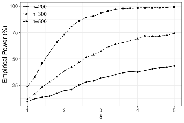
Figure 3: Empirical power of our proposed transfer learning sufficiency test with different target sample size $n$ and signal strength $\delta$. Here we set $p=2000$, $N=400000$, and the significance level $\alpha=0.05$.

3.4. A Real Data Example

To further demonstrate the proposed testing method, we present here a real data example. The target data used here is the Dogs vs.Cats dataset, which is downloadable in the Kaggle competition (https://www.kaggle.com/competitions/dogs-vs-cats/). This dataset contains $n=25,000$ images belonging to two categories (i.e., dogs or cats). The goal here is to classify each image into the two categories, which is denoted by a binary response $Y_{i}$. This is a standard image classification problem, which can be addressed by various deep learning models (Krizhevsky et al., 2012; He et al., 2016; Howard et al., 2017). To demonstrate our method, we first convert the unstructured image data into structured vectors. To this end, various pretrained deep learning models are used. Specifically, we take the feature vectors generated by the last second layer of the pretrained models as our covariate $X_{i}$, whose dimension is usually high. Given the fact that the target sample size is limited as compared with the feature dimension, we turn to transfer learning for help.

We consider the ImageNet dataset (Russakovsky et al., 2014) as our source data. This is a dataset containing a total of $N=1,281,167$ images and covering a total of $K+1=1000$ categories. To convert the images in the source data into structured vectors, the same pretrained deep learning models as for the target data are used. This leads to the high dimensional source covariate $X_{i}^{*}$. Thereafter, a standard multi-class logistic regression model can be fitted for $X_{i}^{*}$ and $Y_{i}^{*}$, where $Y_{i}^{*}\in\{0,1,...,K\}$ indicating the class label for the $i$th image in the source data. This leads to the source data based maximum likelihood estimator $\widehat{\mathbb{B}}_{\text{mle}}^{\text{Source}}$. To transfer information from the source data, a low dimensional feature vector $\widehat{Z}_{i}=\widehat{\mathbb{B}}_{\text{mle}}^{\text{Source}\top}X_{i}\in\mathbb{R}^{K}$ can be constructed for the target data. Thereafter, a standard binary logistic regression model is fitted for $\widehat{Z}_{i}$ and $Y_{i}$. Accordingly, the proposed testing procedure for transfer learning sufficiency can be applied and the prediction accuracy can be evaluated.

For the sake of comprehensive evaluation, a number of classical pretrained deep learning models are used to extract the high dimensional feature vectors $X_{i}$ and $X_{i}^{*}$. They are, respectively, the VGG (Simonyan and Zisserman, 2014) model with two different sizes, the ResNet (He et al., 2016) model with three different sizes, and the InceptionV3 (Szegedy et al., 2016). The resulting feature dimensions are given by $p=4,096$ for the VGG and $p=2,048$ for both the ResNet and InceptionV3. The original target dataset has been randomly split into two parts, among which one is used for training with the sample size 15,000 and the other one is used for testing with the sample size 10,000. The proposed testing procedure for transfer learning sufficiency is then applied on the training dataset. The resulting $p$-values are then reported in Table 2 for every pretrained deep learning model. The prediction accuracy is also evaluated but on the testing dataset. The detailed results are reported in Table 2. By Table 2, we find that the $p$-values of all tests are larger than the significance level $\alpha=0.05$. These results support the null hypostypsis of transfer learning sufficiency. This seems to be very reasonable testing results since the prediction accuracies evaluated on the test dataset are all very high.

Table 2: The $p$-values of the proposed testing procedure and the prediction accuracies on the testing dataset are reported under different pretrained deep learning models.

Model	$p$	$p$-Value	Prediction Accuracy
VGG16	4096	0.846	97.97%
VGG19	4096	0.809	97.93%
ResNet50	2048	0.827	98.06%
ResNet101	2048	0.777	98.40%
ResNet152	2048	0.755	98.50%
InceptionV3	2048	0.691	98.97%

We present here a principled methodology for testing sufficiency of transfer learning. In this regard, a transfer learning estimation procedure is developed and a testing statistic is constructed, whose asymptotic null distribution is analytically derived. Extensive numerical studies are presented to demonstrate the finite sample performance of the proposed method. To conclude this article, we consider here some interesting topics for future study. First, the testing procedure studied in this work requires the sample size of the source data to be much larger than that of the target data. However, in real practice, the sample size of the source data might be comparable with that of the target data. Then how to test for transfer learning sufficiency in this case needs further investigation. Second, if the null hypothesis of transfer learning sufficiency is rejected, how to further improve the estimation accuracy of the target model becomes the next important problem. Last, we use linear transformation in the feature generating function, which might be too restrictive. Then how to test for transfer learning sufficiency with nonlinear feature generating functions is another important problem worthwhile further studying.

APPENDIX

Appendix A. Proof of Theorem 1

Let $\mathbb{U}=(u_{1},\dots,u_{K})\in\mathbb{R}^{p\times K}$ be a matrix with unit length in the sense that $\|\mathbb{U}\|_{F}=1$, where $u_{k}=(u_{k1},\dots,u_{kp})^{\top}\in\mathbb{R}^{p}$ is the $k$th column vector of $\mathbb{U}$. Next, by Fan and Li (2001), it suffices to show that for an arbitrary $\varepsilon>0$, we have

$$\liminf_{n\to\infty}P\Big{\{}\sup_{\|\mathbb{U}\|_{F}=1}\mathcal{L}_{N}^{\text{Source}}\big{(}\mathbb{B}+C\sqrt{p/N}\mathbb{U})<\mathcal{L}_{N}^{\text{Source}}\big{(}\mathbb{B})\Big{\}}\geq 1-\varepsilon$$ (A.1)

for a sufficiently large but fixed constant $C>0$. By Taylor expansion, we have

$$p^{-1}\Big{\{}\mathcal{L}_{N}^{\text{Source}}\Big{(}\mathbb{B}+C\sqrt{p/N}\mathbb{U}\Big{)}-\mathcal{L}_{N}^{\text{Source}}\big{(}\mathbb{B}\big{)}\Big{\}}=C(Np)^{-1/2}\sum_{k=1}^{K}\bigg{(}\frac{\partial\mathcal{L}_{N}^{\text{Source}}(\mathbb{B})}{\partial\beta_{k}}\bigg{)}^{\top}u_{k}$$

$$+2^{-1}C^{2}N^{-1}\sum_{k=1}^{K}\sum_{l=1}^{K}u_{k}^{\top}\Big{(}\frac{\partial^{2}\mathcal{L}_{N}^{\text{Source}}(\mathbb{B})}{\partial\beta_{k}\partial\beta_{l}^{\top}}\Big{)}u_{l}$$

$$+6^{-1}C^{3}p^{1/2}N^{-3/2}\sum_{j=1}^{K}\frac{\partial}{\partial\beta_{j}}\Big{\{}\sum_{k=1}^{K}\sum_{l=1}^{K}u_{k}^{\top}\Big{(}\frac{\partial^{2}\mathcal{L}_{N}^{\text{Source}}(\mathbb{\bar{B}})}{\partial\beta_{k}\partial\beta_{l}^{\top}}\Big{)}u_{l}\Big{\}}^{\top}u_{j},$$ (A.2)

where $\bar{\mathbb{B}}=\mathbb{B}+\nu C\sqrt{p/N}\mathbb{U}$ for some $\nu\in(0,1)$. We next study the three terms in (A.2) separately. By the Cauchy-Schwarz inequality, we have $|\sum_{k=1}^{K}(\partial\mathcal{L}_{N}^{\text{Source}}(\mathbb{B})/\partial\beta_{k})^{\top}u_{k}|\leq\{\sum_{k=1}^{K}\|u_{k}\|^{2}\}^{1/2}\{\sum_{k=1}^{K}\|\partial\mathcal{L}_{N}^{\text{Source}}(\mathbb{B})/\partial\beta_{k}\|^{2}\}^{1/2}=\{\sum_{k=1}^{K}\|\partial\mathcal{L}_{N}^{\text{Source}}(\mathbb{B})/\partial\beta_{k}\|^{2}\}^{1/2}$. Direct computation leads to $E\|\partial\mathcal{L}_{N}^{\text{Source}}(\mathbb{B})/\partial\beta_{k}\|^{2}=E(\sum_{i=1}^{N}\pi_{ik}(1-\pi_{ik})X_{i}^{*\top}X_{i}^{*})\leq NE(X_{i}^{*\top}X_{i}^{*})=NE\{\mbox{tr}(X_{i}^{*\top}X_{i}^{*})\}=N\mbox{tr}\{E(X_{i}^{*}X_{i}^{*\top})\}\leq Np\lambda_{\max}\{E(X_{i}^{*}X_{i}^{*\top})\}=O(Np)$ by Condition (C3). This leads to $\|\partial\mathcal{L}_{N}^{\text{Source}}(\mathbb{B})/\partial\beta_{k}\|=O_{p}(\sqrt{Np})$ . As a consequence, we have $\sqrt{1/Np}\sum_{k=1}^{K}(\partial\mathcal{L}_{N}^{\text{Source}}(\mathbb{B})/\partial\beta_{k})^{\top}u_{k}=O_{p}(1)$. Then we consider the second term of (A.2). For any $\eta>0$ and $k\in\{1,\dots,K\}$, by Chebyshev’s inequality, we have

$$P\bigg{[}\Big{\|}N^{-1}\sum_{i=1}^{N}\pi_{ik}(1-\pi_{ik})X_{i}^{*}X_{i}^{*\top}-E\Big{\{}\pi_{ik}(1-\pi_{ik})X_{i}^{*}X_{i}^{*\top}\Big{\}}\Big{\|}_{F}>\eta\bigg{]}$$

$$\leq\eta^{-2}\sum_{j=1}^{p}\sum_{l=1}^{p}E\bigg{[}N^{-1}\sum_{i=1}^{N}\pi_{ik}(1-\pi_{ik})X_{ij}^{*}X_{il}^{*}-E\Big{\{}\pi_{ik}(1-\pi_{ik})X_{ij}^{*}X_{il}^{*}\Big{\}}\bigg{]}^{2}=O(p^{2}/N).$$

By Condition (C1), we know that $p^{2}/N\leq C^{2}n^{2}/N\to 0$. As a result, we have $\|N^{-1}\sum_{i=1}^{N}\pi_{ik}(1-\pi_{ik})X_{i}^{*}X_{i}^{*\top}-E\{\pi_{ik}(1-\pi_{ik})X_{i}^{*}X_{i}^{*\top}\}\|_{F}=o_{p}(1)$. Similarly, for $k,l\in\{1,\dots,K\}$ and $k\neq l$, we can show that $\|N^{-1}\sum_{i=1}^{N}\pi_{ik}\pi_{il}X_{i}^{*}X_{i}^{*\top}-E(\pi_{ik}\pi_{il}X_{i}^{*}X_{i}^{*\top})\|_{F}=o_{p}(1)$. Recall that $W_{i}=\mbox{diag}(\pi_{i})-\pi_{i}\pi_{i}^{\top}\in\mathbb{R}^{K\times K}$ with $\pi_{i}=(\pi_{i1},\dots,\pi_{iK})^{\top}$ and $\pi_{ik}=P(Y_{i}^{*}=k|X_{i}^{*})$. Combining the above results, we have

$$\begin{split}&\lambda_{\min}^{2}\bigg{[}N^{-1}\sum_{i=1}^{N}W_{i}\otimes\big{(}X_{i}^{*}X_{i}^{*\top}\big{)}-E\Big{\{}W_{i}\otimes\big{(}X_{i}^{*}X_{i}^{*\top}\big{)}\Big{\}}\bigg{]}\\ \leq&\Big{\|}N^{-1}\sum_{i=1}^{N}W_{i}\otimes\big{(}X_{i}^{*}X_{i}^{*\top}\big{)}-E\Big{\{}W_{i}\otimes\big{(}X_{i}^{*}X_{i}^{*\top}\big{)}\Big{\}}\Big{\|}_{F}^{2}\\ =&\sum_{k=1}^{K}\Big{\|}N^{-1}\sum_{i=1}^{N}\pi_{ik}(1-\pi_{ik})X_{i}^{*}X_{i}^{*\top}-E\Big{\{}\pi_{ik}(1-\pi_{ik})X_{i}^{*}X_{i}^{*\top}\Big{\}}\Big{\|}_{F}^{2}\\ +&\sum_{k\neq l}\Big{\|}N^{-1}\sum_{i=1}^{N}\pi_{ik}\pi_{il}X_{i}^{*}X_{i}^{*\top}-E\Big{(}\pi_{ik}\pi_{il}X_{i}^{*}X_{i}^{*\top}\Big{)}\Big{\|}_{F}^{2}=o_{p}(1)\end{split}$$

By Weyl’s inequality (Seber, 2008), we know that $\lambda_{\min}(A+B)\geq\lambda_{\min}(A)+\lambda_{\min}(B)$ for any two symmetric matrices $A$ and $B$. As a result, for the second term of (A.2), we have

$$\begin{split}&-N^{-1}\sum_{k=1}^{K}\sum_{l=1}^{K}u_{k}^{\top}\frac{\partial^{2}\mathcal{L}_{N}^{\text{Source}}(\mathbb{B})}{\partial\beta_{k}\partial\beta_{l}^{\top}}u_{l}-\lambda_{\min}\bigg{[}E\Big{\{}W_{i}\otimes\big{(}X_{i}^{*}X_{i}^{*\top}\big{)}\Big{\}}\bigg{]}\\ =&\mathrm{vec}(\mathbb{U})^{\top}\Big{\{}N^{-1}\sum_{i=1}^{N}W_{i}\otimes\big{(}X_{i}^{*}X_{i}^{*\top}\big{)}\Big{\}}\mathrm{vec}(\mathbb{U})-\lambda_{\min}\bigg{[}E\Big{\{}W_{i}\otimes\big{(}X_{i}^{*}X_{i}^{*\top}\big{)}\Big{\}}\bigg{]}\\ \geq&\lambda_{\min}\Big{\{}N^{-1}\sum_{i=1}^{N}W_{i}\otimes\big{(}X_{i}^{*}X_{i}^{*\top}\big{)}\Big{\}}-\lambda_{\min}\bigg{[}E\Big{\{}W_{i}\otimes\big{(}X_{i}^{*}X_{i}^{*\top}\big{)}\Big{\}}\bigg{]}\\ \geq&\lambda_{\min}\bigg{[}N^{-1}\sum_{i=1}^{N}W_{i}\otimes\big{(}X_{i}^{*}X_{i}^{*\top}\big{)}-E\Big{\{}W_{i}\otimes\big{(}X_{i}^{*}X_{i}^{*\top}\big{)}\Big{\}}\bigg{]}\stackrel{{\scriptstyle p}}{{\to}}0.\end{split}$$ (A.3)

By the Condition (C3), we know that $E\{W_{i}\otimes(X_{i}^{*}X_{i}^{*\top})\}$ is a positive definite matrix with $\lambda_{\min}\{E(W_{i}\otimes X_{i}^{*}X_{i}^{*\top})\}\geq C_{\min}$ for some positive constant $C_{\min}>0$. As a consequence, we have $-N^{-1}\sum_{k=1}^{K}\sum_{l=1}^{K}u_{k}^{\top}\partial^{2}\mathcal{L}_{N}^{\text{Source}}(\mathbb{B})/\partial\beta_{k}\partial\beta_{l}^{\top}u_{l}>0$ with probability tending to one. For the third term of (A.2), by Cauchy-Schwarz inequality,

$$\Big{|}\frac{\partial}{\partial\beta_{j}}\Big{\{}\sum_{k=1}^{K}\sum_{l=1}^{K}u_{k}^{\top}\Big{(}\frac{\partial^{2}\mathcal{L}_{N}^{\text{Source}}(\mathbb{\bar{B}})}{\partial\beta_{k}\partial\beta_{l}^{\top}}\Big{)}u_{l}\Big{\}}^{\top}u_{j}\Big{|}=\Big{|}\sum_{k=1}^{K}\sum_{l=1}^{K}\sum_{i=1}^{N}\Big{(}\frac{\partial p_{ikl}}{\partial\beta_{j}}\Big{)}^{\top}u_{j}\Big{(}X_{i}^{*\top}u_{k}\Big{)}\Big{(}X_{i}^{*\top}u_{l}\Big{)}\Big{|}$$

$$\leq\sum_{k=1}^{K}\sum_{l=1}^{K}\sup_{i}\Big{\|}\frac{\partial p_{ikl}}{\partial\beta_{j}}\Big{|}_{\beta_{j}=\bar{\beta}_{j}}\Big{\|}\Big{\{}\sum_{i=1}^{N}(u_{k}^{\top}X_{i}^{*}X_{i}^{*\top}u_{k})\Big{\}}^{1/2}\Big{\{}\sum_{i=1}^{N}(u_{l}^{\top}X_{i}^{*}X_{i}^{*\top}u_{l})\Big{\}}^{1/2},$$

where $p_{ikl}=\pi_{ik}(1-\pi_{ik})$ if $k=l$ and $p_{ikl}=-\pi_{ik}\pi_{il}$ if $k\neq l$. By simple computation, in the case of $k=l$, we have $\partial p_{ikl}/\partial\beta_{j}=\pi_{ik}(1-\pi_{ik})(1-2\pi_{ik})X_{i}^{*}$ if $j=k=l$, and $\partial p_{ikl}/\partial\beta_{j}=-\pi_{ik}\pi_{ij}(1-2\pi_{ik})X_{i}^{*}$ if $j\neq k$. In the case of $k\neq l$, we have $\partial p_{ikl}/\partial\beta_{j}=2\pi_{ik}\pi_{il}\pi_{ij}X_{i}^{*}$ if $j\neq k$, and $j\neq l$ and $\partial p_{ikl}/\partial\beta_{j}=-\pi_{ik}\pi_{il}(1-2\pi_{ij})X_{i}^{*}$ if $j=k$ or $j=l$. In all cases, we have $\sup_{i}\|\partial p_{ikl}/\partial\beta_{j}\|\leq 2\sup_{i}\|X_{i}^{*}\|$. Note that by Condition (C2), we know that each component of $X_{i}^{*}$ is sub-Gaussian. Thus, by Proposition 2.5.2 in Vershynin (2018), we know that $E\exp(X_{ij}^{*2}/\|X^{*}_{ij}\|_{\psi_{2}}^{2})\leq 2$. Let $j^{*}_{i}=\max\{j:X_{ij}^{*2}/\|X^{*}_{ij}\|_{\psi_{2}}^{2}\}$. Then by the fact that $\|X_{i}^{*}\|_{\psi_{2}}\geq\|X^{*}_{ij}\|_{\psi_{2}}$, we have $E\exp\{\|X_{i}^{*}\|^{2}/(p\|X_{i}^{*}\|_{\psi_{2}}^{2})\}\leq E\exp(X_{ij^{*}}^{*2}/\|X^{*}_{ij^{*}}\|_{\psi_{2}}^{2})\leq 2$. Then we know that $\|X_{i}^{*}\|/\sqrt{p}$ is sub-Gaussian. By the results of Exercise 2.5.10 in Vershynin (2018), we then have $\sup_{i}\|X_{i}^{*}\|=O_{p}(\sqrt{p\log N})$. As a result, we have $\sup_{i}\|\partial p_{ikl}/\partial\beta_{j}\|=O_{p}(\sqrt{p\log N})$. By a similar proof of (LABEL:min_eigen), we know that $\lambda_{\max}(N^{-1}\sum_{i=1}^{N}X_{i}^{*}X_{i}^{*\top})-\lambda_{\max}\{E(X_{i}^{*}X_{i}^{*\top})\}\stackrel{{\scriptstyle p}}{{\to}}0$. By Condition (C3), we know that $\lambda_{\max}\{E(X_{i}^{*}X_{i}^{*\top})\}\leq C_{\max}$. Note that $\|u_{k}\|\leq 1$. Then we have $N^{-1}\sum_{i=1}^{N}u_{k}^{\top}X_{i}^{*}X_{i}^{*\top}u_{k}\leq\lambda_{\max}(N^{-1}\sum_{i=1}^{N}X_{i}^{*}X_{i}^{*\top})=O_{p}(1)$. As a result, we have $\sum_{i=1}^{N}u_{k}^{\top}X_{i}^{*}X_{i}^{*\top}u_{k}=O_{p}(N)$. Consequently, by Condition (C1), the third term of (A.2) is of the order $p^{1/2}N^{-3/2}O_{p}(\sqrt{p\log N})O_{p}(N)=O_{p}(\sqrt{p^{2}\log N/N})=O_{p}(\sqrt{n^{2}\log N/N})=o_{p}(1)$. Then we can choose a sufficiently large $C$ such that $\mathcal{L}_{N}^{\text{Source}}(\mathbb{B}+C\sqrt{p/N}\mathbb{U})-\mathcal{L}_{N}^{\text{Source}}(\mathbb{B})<0$, which completes the theorem proof.

Appendix B. Proof of Theorem 2

The theorem conclusion can be established in three steps. In the first step, we show that there exists a local optimizer $\widehat{\gamma}$, which is $\sqrt{n}$-consistent. In the second step, we study the asymptotic normality of $\widehat{\gamma}$. In the third step, we analyse the asymptotic behavior of $\widehat{\theta}^{\text{Transfer}}$.

Step 1. $\sqrt{n}$-consistency

Recall that $\mathcal{L}_{n}(\gamma;\widehat{Z})=\sum_{i=1}^{n}[Y_{i}(\widehat{Z}_{i}^{\top}\gamma)-\log\{1+\exp(\widehat{Z}_{i}^{\top}\gamma)\}]$ is the working log-likelihood. By Fan and Li (2001), we would like to show that, for an arbitrary but fixed $\varepsilon>0$, we have

$$\liminf_{n\to\infty}P\Big{\{}\sup_{\|u\|=1}\mathcal{L}_{n}\big{(}\gamma+C_{\varepsilon}n^{-1/2}u;\widehat{Z}\big{)}<\mathcal{L}_{n}\big{(}\gamma;\widehat{Z}\big{)}\Big{\}}\geq 1-\varepsilon,$$ (B.1)

for a sufficiently large constant $C_{\varepsilon}>0$. To this end, Taylor expansion is applied as

$$\mathcal{L}_{n}\Big{(}\gamma+C_{\varepsilon}n^{-1/2}u;\widehat{Z}\Big{)}-\mathcal{L}_{n}\Big{(}\gamma;\widehat{Z}\Big{)}$$

$$=C_{\varepsilon}n^{-1/2}\dot{\mathcal{L}}_{n}(\gamma;\widehat{Z})^{\top}u-2^{-1}C_{\varepsilon}^{2}u^{\top}\Big{\{}-n^{-1}\ddot{\mathcal{L}}_{n}(\gamma;\widehat{Z})\Big{\}}u+o_{p}(1),$$ (B.2)

where $\dot{\mathcal{L}}_{n}(\gamma,\widehat{Z})$ and $\ddot{\mathcal{L}}_{n}(\gamma,\widehat{Z})$ are the first-order and second-order partial derivative of the working log-likelihood function $\mathcal{L}_{n}(\gamma;\widehat{Z})$ with respect to $\gamma$, respectively. To verify (B.1), it suffices to show the following two key results:

$$(1)\sup_{\|u\|=1}n^{-1/2}\dot{\mathcal{L}}_{n}(\gamma;\widehat{Z})^{\top}u=O_{p}(1),$$ (B.3)

$$(2)\lambda_{\min}\{-n^{-1}\ddot{\mathcal{L}}_{n}(\gamma;\widehat{Z})\}\geq\tau_{\min}>0,$$ (B.4)

for some positive constant $\tau_{\min}$ with probability tending to one. Then we verify the conclusions by the following two sub-steps.

Step 1.1. We start with (B.3). Direct computation leads to $n^{-1/2}\dot{\mathcal{L}}_{n}(\gamma,\widehat{Z})^{\top}u=n^{-1/2}\dot{\mathcal{L}}_{n}(\gamma,Z)^{\top}u+n^{-1/2}\{\dot{\mathcal{L}}_{n}(\gamma,\widehat{Z})-\dot{\mathcal{L}}_{n}(\gamma,Z)\}^{\top}u$. The first term $n^{-1/2}\dot{\mathcal{L}}_{n}(\gamma,Z)^{\top}u$ can be uniformly bounded by $n^{-1/2}\|\dot{\mathcal{L}}_{n}(\gamma,Z)\|=O_{p}(1)$; see Fan and Li (2001). We thus focus on the second term. By mean value theorem and Cauchy-Schwarz inequality, we can verify that

$$\bigg{|}n^{-1/2}\Big{\{}\dot{\mathcal{L}}_{n}(\gamma,\widehat{Z})-\dot{\mathcal{L}}_{n}(\gamma,Z)\Big{\}}^{\top}u\bigg{|}\leq\sum_{i=1}^{n}\bigg{|}n^{-1/2}g\Big{(}\xi_{i}^{\top}\gamma\Big{)}\Big{\{}1-g\Big{(}\xi_{i}^{\top}\gamma\Big{)}\Big{\}}(\widehat{Z}_{i}-Z_{i})^{\top}\xi_{i}\gamma^{\top}u\bigg{|}$$

$$+\sum_{i=1}^{n}\bigg{|}n^{-1/2}\Big{\{}Y_{i}-g\Big{(}\xi_{i}^{\top}\gamma\Big{)}\Big{\}}(\widehat{Z}_{i}-Z_{i})^{\top}u\bigg{|}$$

$$\leq\sqrt{n}\Big{\{}n^{-1}\sum_{i=1}^{n}\|\widehat{Z}_{i}-Z_{i}\|^{2}\Big{\}}^{1/2}\bigg{[}n^{-1}\sum_{i=1}^{n}\Big{\|}g\Big{(}\xi_{i}^{\top}\gamma\Big{)}\Big{\{}1-g\Big{(}\xi_{i}^{\top}\gamma\Big{)}\Big{\}}\xi_{i}\Big{\|}^{2}\bigg{]}^{1/2}\|\gamma\|$$

$$+\bigg{\{}\sum_{i=1}^{n}\Big{|}Y_{i}-g\Big{(}\xi_{i}^{\top}\gamma\Big{)}\Big{|}^{2}\bigg{\}}^{1/2}\Big{\{}n^{-1}\sum_{i=1}^{n}\|\widehat{Z}_{i}-Z_{i}\|^{2}\Big{\}}^{1/2},$$ (B.5)

where $\xi_{i}=\eta_{i}\widehat{Z}_{i}+(1-\eta_{i})Z_{i}$ for some $\eta_{i}\in(0,1)$. We first evalutate the first term of (B.5). Simple computation leads to $n^{-1}\sum_{i=1}^{n}\|\widehat{Z}_{i}-Z_{i}\|^{2}=n^{-1}\sum_{i=1}^{n}\|(\widehat{\mathbb{B}}-\mathbb{B})^{\top}X_{i}\|^{2}=\sum_{k=1}^{K}(\widehat{\beta}_{k}-\beta_{k})^{\top}(n^{-1}\sum_{i=1}^{n}X_{i}X_{i}^{\top})(\widehat{\beta}_{k}-\beta_{k})\leq\lambda_{\max}(n^{-1}\sum_{i=1}^{n}X_{i}X_{i}^{\top})\sum_{k=1}^{K}\|\widehat{\beta}_{k}-\beta_{k}\|^{2}$. In the meanwhile, by Theorem 6.5 in Wainwright (2019) and Condition (C1), we know that there exists some constant $C_{1}>0$ such that $\lambda_{\max}\{n^{-1}\sum_{i=1}^{n}X_{i}X_{i}^{\top}-E(X_{i}X_{i}^{\top})\}\leq C_{1}(\sqrt{p/n}+p/n)\leq C_{1}(\sqrt{C}+C)$ with probability tending to one. Then by Condition (C3), we have $\lambda_{\max}(n^{-1}\sum_{i=1}^{n}X_{i}X_{i}^{\top})\leq C_{1}(\sqrt{C}+C)+\lambda_{\max}\{E(X_{i}X_{i}^{\top})\}\leq C_{1}(\sqrt{C}+C)+C_{\max}$ with probability tending to one. That is, $\lambda_{\max}(n^{-1}\sum_{i=1}^{n}X_{i}X_{i}^{\top})=O_{p}(1)$. By Theorem 1, we have $\|\widehat{\beta}_{k}-\beta_{k}\|=O_{p}(\sqrt{p/N})$ for $k=1,\dots,K$. As a consequence, we have $n^{-1}\sum_{i=1}^{n}\|\widehat{Z}_{i}-Z_{i}\|^{2}=O_{p}(p/N)$. Furthermore, note that $\xi_{i}=\eta_{i}(\widehat{Z}_{i}-Z_{i})+Z_{i}$. By Condition (C4), we know that $E\|Z_{i}\|^{2}\leq\{E\|Z_{i}\|^{4}\}^{1/2}\leq\tau_{\max}^{1/2}$. We then have $n^{-1}\sum_{i=1}^{n}\|g(\xi_{i}^{\top}\gamma)\{1-g(\xi_{i}^{\top}\gamma)\}\xi_{i}\|^{2}\leq n^{-1}\sum_{i=1}^{n}\|\xi_{i}\|^{2}\leq 2n^{-1}\sum_{i=1}^{n}(\|Z_{i}\|^{2}+\|\eta_{i}(\widehat{Z}_{i}-Z_{i})\|^{2})=O_{p}(1)$. As a consequence, the first term of (B.5) is of order $O_{p}(\sqrt{np/N})$. Then we consider the second term of (B.5). We have $\{\sum_{i=1}^{n}|Y_{i}-g(\xi_{i}^{\top}\gamma)|^{2}\}^{1/2}\leq\sqrt{n}$ since $|Y_{i}-g(\xi_{i}^{\top}\gamma)|\leq 1$. Note that $n^{-1}\sum_{i=1}^{n}\|\widehat{Z}_{i}-Z_{i}\|^{2}=O_{p}(p/N)$. Then the second term of (B.5) is of order $O_{p}(\sqrt{np/N})$. Combining all the preceding results, we obtain that $|n^{-1/2}\{\dot{\mathcal{L}}_{n}(\gamma,\widehat{Z})-\dot{\mathcal{L}}_{n}(\gamma,Z)\}^{\top}u|=O_{p}(\sqrt{np/N})$. By Condition (C1) we know that $np/N\leq Cn^{2}/N\to 0$. Then we have $n^{-1/2}\dot{\mathcal{L}}_{n}(\gamma,\widehat{Z})^{\top}u=n^{-1/2}\dot{\mathcal{L}}_{n}(\gamma,Z)^{\top}u+o_{p}(1)=O_{p}(1)$. This proves (B.3).

Step 1.2. We next study (B.4). Recall $I(\gamma)=-E\{n^{-1}\ddot{\mathcal{L}}_{n}(\gamma,Z)\}$ is the Fisher information matrix of the oracle likelihood. Then $\eqref{Ln Taylor second}$ follows if we can show that

$$\sup_{\|u\|=1}\Big{|}u^{\top}\Big{\{}-n^{-1}\ddot{\mathcal{L}}_{n}(\gamma;\widehat{Z})-I(\gamma)\Big{\}}u\Big{|}\leq\sup_{\|u\|=1}\Big{|}n^{-1}u^{\top}\ddot{\mathcal{L}}_{n}(\gamma;\widehat{Z})u-n^{-1}u^{\top}\ddot{\mathcal{L}}_{n}(\gamma;Z)u\Big{|}$$

$$+\sup_{\|u\|=1}\Big{|}u^{\top}\Big{\{}-n^{-1}\ddot{\mathcal{L}}_{n}(\gamma;Z)-I(\gamma)\Big{\}}u\Big{|}=o_{p}(1).$$ (B.6)

By Law of Large Numbers, we have $-n^{-1}\ddot{\mathcal{L}}_{n}(\gamma;Z)\stackrel{{\scriptstyle p}}{{\to}}I(\gamma)$. As a result, (B.4) follows if we can show that $\sup_{\|u\|=1}n^{-1}u^{\top}\{\ddot{\mathcal{L}}_{n}(\gamma;\widehat{Z})-\ddot{\mathcal{L}}_{n}(\gamma;Z)\}u=o_{p}(1)$. By the mean value theorem, we can write

$$\Big{|}u^{\top}\Big{\{}n^{-1}\ddot{\mathcal{L}}_{n}(\gamma;\widehat{Z})-n^{-1}\ddot{\mathcal{L}}_{n}(\gamma;Z)\Big{\}}u\Big{|}$$

$$= n^{-1}\bigg{|}\sum_{i=1}^{n}\bigg{[}g\Big{(}\widehat{Z}_{i}^{\top}\gamma\Big{)}\Big{\{}1-g\Big{(}\widehat{Z}_{i}^{\top}\gamma\Big{)}\Big{\}}\Big{(}\widehat{Z}_{i}^{\top}u\Big{)}^{2}-g\Big{(}Z_{i}^{\top}\gamma\Big{)}\Big{\{}1-g\Big{(}Z_{i}^{\top}\gamma\Big{)}\Big{\}}\Big{(}Z_{i}^{\top}u\Big{)}^{2}\bigg{]}\bigg{|}$$

$$= \bigg{[}\Big{\{}1-2g\Big{(}\tilde{\xi}_{i}^{\top}\gamma\Big{)}\Big{\}}g\Big{(}\tilde{\xi}_{i}^{\top}\gamma\Big{)}\Big{\{}1-g\Big{(}\tilde{\xi}_{i}^{\top}\gamma\Big{)}\Big{\}}\Big{(}\tilde{\xi}_{i}^{\top}u\Big{)}^{2}\gamma+2g\Big{(}\tilde{\xi}^{\top}\gamma\Big{)}\Big{\{}1-g\Big{(}\tilde{\xi}_{i}^{\top}\gamma\Big{)}\Big{\}}\Big{(}\tilde{\xi}_{i}^{\top}u\Big{)}u\bigg{]}$$

$$\times n^{-1}\bigg{|}\sum_{i=1}^{n}\Big{(}\widehat{Z}_{i}-Z_{i}\Big{)}^{\top}\bigg{|}\leq\Big{\{}n^{-1}\sum_{i=1}^{n}\|\widehat{Z}_{i}-Z_{i}\|^{2}\Big{\}}^{1/2}\times\Big{(}I_{1}+I_{2}\Big{)}=O_{p}(\sqrt{p/N})(I_{1}+I_{2}),$$

where $I_{1}=\big{\{}n^{-1}\sum_{i=1}^{n}\big{\|}\big{\{}1-2g\big{(}\tilde{\xi}_{i}^{\top}\gamma\big{)}\big{\}}g\big{(}\tilde{\xi}_{i}^{\top}\gamma\big{)}\big{\{}1-g\big{(}\tilde{\xi}_{i}^{\top}\gamma\big{)}\big{\}}\big{(}\tilde{\xi}_{i}^{\top}u\big{)}^{2}\gamma\big{\|}^{2}\big{\}}^{1/2}$, $I_{2}=\big{\{}n^{-1}\sum_{i=1}^{n}\\ \big{\|}2g\big{(}\tilde{\xi}^{\top}\gamma\big{)}\big{\{}1-g\big{(}\tilde{\xi}_{i}^{\top}\gamma\big{)}\big{\}}\big{(}\tilde{\xi}_{i}^{\top}u\big{)}u\big{\|}^{2}\big{\}}^{1/2}$, and $\tilde{\xi}_{i}=\tilde{\eta}_{i}\widehat{Z}_{i}+(1-\tilde{\eta}_{i})Z_{i}$ for some $\tilde{\eta}_{i}\in[0,1]$. Next, we should evaluate $I_{1}$ and $I_{2}$ sequentially. For $I_{1}$, we can verify that $I_{1}^{2}\leq n^{-1}\|\gamma\|^{2}\sum_{i=1}^{n}(\tilde{\xi}_{i}^{\top}u)^{2}\leq n^{-1}\|\gamma\|^{2}\sum_{i=1}^{n}\|\tilde{\xi}_{i}\|^{2}$ The first inequality holds by the following results: (a) $|g(\tilde{\xi}_{i}^{\top}\tilde{\gamma})\{1-g(\tilde{\xi}_{i}^{\top}\tilde{\gamma})\}|\leq 1$ and (b) $|1-2g(\tilde{\xi}_{i}^{\top}\tilde{\gamma})|\leq 1$. Then by a similar procedure as in Step 1.1, we have $n^{-1}\sum_{i=1}^{n}\|\tilde{\xi}_{i}\|^{2}=O_{p}(1)$. Note that by assuming $\gamma$ is bounded, we have $I_{1}=O_{p}(1)$. For $I_{2}$, by similar argument above, we can show that $I_{2}^{2}\leq n^{-1}\sum_{i=1}^{n}\|\tilde{\xi}_{i}\|^{2}=O_{p}(1)$. Thus, the first term of (B.6) is bounded by $O_{p}(\sqrt{p/N})=o_{p}(1)$. Combining the above results, we have $\sup_{\|u\|=1}|-n^{-1}u^{\top}\ddot{\mathcal{L}}_{n}(\gamma;\widehat{Z})u-u^{\top}I(\gamma)u|=o_{p}(1)$ and $\inf_{\|u\|=1}\big{\{}-n^{-1}u^{\top}\ddot{\mathcal{L}}_{n}(\gamma;\widehat{Z})u\big{\}}\geq\inf_{\|u\|=1}\big{\{}-n^{-1}u^{\top}\ddot{\mathcal{L}}_{n}(\gamma;\widehat{Z})u-u^{\top}I(\gamma)u\big{\}}\\ +\inf_{\|u\|=1}\big{\{}u^{\top}I(\gamma)u\big{\}}=o_{p}(1)+\lambda_{\min}\{I(\gamma)\}.$ Note that $I(\gamma)$ is a positive definite matrix whose eigenvalues are bounded away from zero. Consequently, we have $\lambda_{\min}\{I(\gamma)\}>0$. As a consequence, we have $\lambda_{\min}\{n^{-1}u^{\top}\ddot{\mathcal{L}}_{n}(\gamma;\widehat{Z})u\}=\inf_{\|u\|=1}\{n^{-1}u^{\top}\ddot{\mathcal{L}}_{n}(\gamma;\widehat{Z})u\}>2^{-1}\lambda_{\min}\{I(\gamma)\}$ with probability tending to one. Thus, for the $\varepsilon$ mentioned above, we can take a sufficiently large $C_{\varepsilon}$ such that $\sup_{\|u\|=1}\mathcal{L}_{n}(\gamma+C_{\varepsilon}n^{-1/2}u;\widehat{Z})<\mathcal{L}_{n}(\gamma;\widehat{Z})$. Combining the preceding steps, we complete the proof of $\sqrt{n}$-consistency.

Step 2. Asymptotic Normality

We next study the asymptotic distribution of $\widehat{\gamma}$. Note that $\widehat{\gamma}$ is a local optimizer of $\mathcal{L}_{n}(\gamma;\widehat{Z})$. We then should have $\dot{\mathcal{L}}_{n}(\gamma;\widehat{Z})=0$. Recall that $\widehat{\gamma}$ is $\sqrt{n}$-consistent for $\gamma$. We can then apply Taylor’s expansion at $\gamma$. This leads to

$$0=n^{-1/2}\dot{\mathcal{L}}_{n}(\widehat{\gamma};\widehat{Z})=n^{-1/2}\dot{\mathcal{L}}_{n}(\gamma;\widehat{Z})+n^{-1}\ddot{\mathcal{L}}_{n}(\gamma;\widehat{Z})\sqrt{n}(\widehat{\gamma}-\gamma)+o_{p}(1).$$ (B.7)

Then we verify the asymptotic normality of $\widehat{\gamma}$ by the following two conclusions: (a) $n^{-1/2}\dot{\mathcal{L}}_{n}(\gamma;\widehat{Z})\stackrel{{\scriptstyle d}}{{\to}}N(0,I(\gamma))$; and (b) $-n^{-1}\ddot{\mathcal{L}}_{n}(\gamma;\widehat{Z})\stackrel{{\scriptstyle p}}{{\to}}I(\gamma)$. We next prove the two above conclusions separately.

Step 2.1. We start with the asymptotic normality of $n^{-1/2}\dot{\mathcal{L}}_{n}(\gamma;\widehat{Z})$. Simple computation leads to $n^{-1/2}\dot{\mathcal{L}}_{n}(\gamma;\widehat{Z})=n^{-1/2}\dot{\mathcal{L}}_{n}(\gamma;Z)+n^{-1/2}\{\dot{\mathcal{L}}_{n}(\gamma;\widehat{Z})-\dot{\mathcal{L}}_{n}(\gamma;Z)\}$. By Central Limit Theorem, we have $n^{-1/2}\dot{\mathcal{L}}_{n}(\gamma;Z)\stackrel{{\scriptstyle d}}{{\to}}N(0,I(\gamma))$. By a similar procedure in Step 1.1 and the property of $\ell_{2}$ norm, we have $n^{-1/2}\|\dot{\mathcal{L}}_{n}(\gamma;\widehat{Z})-\dot{\mathcal{L}}_{n}(\gamma;Z)\|=\sup_{\|u\|=1}n^{-1/2}\|\{\dot{\mathcal{L}}_{n}(\gamma;\widehat{Z})-\dot{\mathcal{L}}_{n}(\gamma;Z)\}^{\top}u\|=o_{p}(1)$. Combining the above two results, we have $n^{-1/2}\dot{\mathcal{L}}_{n}(\gamma;\widehat{Z})\stackrel{{\scriptstyle d}}{{\to}}N(0,I(\gamma))$.

Step 2.2. We show consistency of $-n^{-1}\ddot{\mathcal{L}}_{n}(\gamma;\widehat{Z})$. For an arbitrary matrix $A=(a_{ij})\in\mathbb{R}^{m\times n}$, define its spectral norm as $\|A\|_{2}=\sqrt{\lambda_{\max}(A^{\top}A)}$. By (B.6), we have

$$\Big{\|}-n^{-1}\ddot{\mathcal{L}}_{n}(\gamma;\widehat{Z})-I(\gamma)\Big{\|}_{2}=\sup_{\|u\|=1}\Big{|}u^{\top}\Big{\{}-n^{-1}\ddot{\mathcal{L}}_{n}(\gamma;\widehat{Z})-I(\gamma)\Big{\}}u\Big{|}=o_{p}(1).$$

Consequently, we have $-n^{-1}\ddot{\mathcal{L}}_{n}(\gamma;\widehat{Z})\stackrel{{\scriptstyle p}}{{\to}}I(\gamma)$. Then $n^{-1}\ddot{\mathcal{L}}_{n}(\gamma;\widehat{Z})$ is invertible with probability tending to one. As a result, by Slutsky’s theorem, we have $\sqrt{n}(\widehat{\gamma}-\gamma)=\{-n^{-1}\ddot{\mathcal{L}}_{n}(\gamma;\widehat{Z})\}^{-1}\{n^{-1/2}\dot{\mathcal{L}}_{n}(\gamma;\widehat{Z})\}+o_{p}(1)\stackrel{{\scriptstyle d}}{{\to}}N(0,I(\gamma)^{-1}).$ This completes the proof of asymptotic normality of $\widehat{\gamma}$.

Step 3. Consistency and Asymptotic Normality of $\widehat{\theta}^{\text{Transfer}}$

We next study the asymptotic behavior of $\widehat{\theta}^{\text{Transfer}}$. The proof includes two parts. In the first part, we verify the $\sqrt{n}$-consistency of $\widehat{\theta}^{\text{Transfer}}$, while in the second part, we shown the asymptotic normality of $\widehat{\theta}^{\text{Transfer}}$.

Step 3.1. We start with the $\sqrt{n}$-consistency. By Cauchy-Schwarz inequality and the property of operator norm (Seber, 2008), we have $||\widehat{\theta}^{\text{Transfer}}-\theta||\leq||\widehat{\mathbb{B}}_{\text{mle}}^{\text{Source}}-\mathbb{B}||_{F}||\widehat{\gamma}||+\lambda_{\max}^{1/2}(\mathbb{B}^{\top}\mathbb{B})||\widehat{\gamma}-\gamma||$. Recall that we have shown $\widehat{\gamma}-\gamma=O_{p}(1/\sqrt{n})$ in Step 1. By Theorem 1, the first term is of order $O_{p}(\sqrt{p/N})\{\gamma+O_{p}(1/\sqrt{n})\}=O_{p}(\sqrt{p/N})$. Then by Condition (C5), we know the second term is of order $O(1)O_{p}(1/\sqrt{n})=O_{p}(1/\sqrt{n})$. Furthermore, given $n^{2}\log N/N\to 0$ and $p\leq Cn$ by Condition (C1), we can obtain $||\widehat{\theta}^{\text{Transfer}}-\theta||=O_{p}(1/\sqrt{n})$ and thus $\widehat{\theta}^{\text{Transfer}}$ is $\sqrt{n}$-consistent.

Step 3.2. Then we evaluate the asymptotic normality of $\widehat{\theta}^{\text{Transfer}}$. By the theorem condition $v\in\mathcal{S}(\mathbb{B})$ , there exists a vector $\zeta\in\mathbb{R}^{K}$ such that $v=\mathbb{B}\zeta$. As a result, we have $\sigma^{2}(v)=v^{\top}\mathbb{B}I^{-1}(\gamma)\mathbb{B}^{\top}v=\zeta^{\top}\mathbb{B}^{\top}\mathbb{B}I^{-1}(\gamma)\mathbb{B}^{\top}\mathbb{B}\zeta\geq\lambda_{\max}^{-1}\{I(\gamma)\}\lambda_{\min}\{\mathbb{B}^{\top}\mathbb{B}\}$. Similarly, we have $\sigma^{2}(v)\leq\lambda_{\min}^{-1}\{I(\gamma)\}\lambda_{\max}(\mathbb{B}^{\top}\mathbb{B})$. By Condition (C5) and the positive definiteness of $I(\gamma)$ and $\mathbb{B}^{\top}\mathbb{B}$, we have $\sigma^{2}(v)=O(1)$ and $\sigma^{-2}(v)=O(1)$. Note that $\sqrt{n}v^{\top}(\widehat{\theta}^{\text{Transfer}}-\theta)/\sigma(v)=\sqrt{n}v^{\top}(\widehat{\mathbb{B}}_{\text{mle}}^{\text{Source}}-\mathbb{B})\widehat{\gamma}/\sigma(v)+\sqrt{n}v^{\top}\mathbb{B}(\widehat{\gamma}-\gamma)/\sigma(v)$. By Condition (C1), Theorem 1, and Cauchy-Schwarz inequality, we know that $\sqrt{n}v^{\top}(\widehat{\mathbb{B}}_{\text{mle}}^{\text{Source}}-\mathbb{B})\widehat{\gamma}/\sigma(v)\leq\sqrt{n}\|v\|\|\widehat{\mathbb{B}}_{\text{mle}}^{\text{Source}}-\mathbb{B}\|_{F}\|\widehat{\gamma}\|/\sigma(v)=\sqrt{n}O_{p}(\sqrt{p/N})O_{p}(1)=O_{p}(\sqrt{np/N})=O_{p}(\sqrt{n^{2}/N})=o_{p}(1)$. Note that $\|\mathbb{B}^{\top}v\|\leq\lambda_{\max}(\mathbb{B}^{\top}\mathbb{B})\leq\tau_{\max}$. By the results in Step 1.1, (B.6) and (B.7), we know that

$$0=n^{-1/2}\sigma^{-1}(v)v^{\top}\mathbb{B}\Big{\{}-n^{-1}\ddot{\mathcal{L}}_{n}(\gamma;\widehat{Z})\Big{\}}^{-1}\dot{\mathcal{L}}_{n}(\gamma;\widehat{Z})-\sqrt{n}\sigma^{-1}(v)v^{\top}\mathbb{B}(\widehat{\gamma}-\gamma)+o_{p}(1)$$

$$=n^{-1/2}\sigma^{-1}(v)v^{\top}\mathbb{B}I(\gamma)^{-1}\dot{\mathcal{L}}_{n}(\gamma;Z)-\sqrt{n}\sigma^{-1}(v)v^{\top}\mathbb{B}(\widehat{\gamma}-\gamma)+o_{p}(1)$$

$$=\sum_{i=1}^{n}Y_{ni}-\sqrt{n}\sigma^{-1}(v)v^{\top}\mathbb{B}(\widehat{\gamma}-\gamma)+o_{p}(1),$$ (B.8)

where $Y_{ni}=n^{-1/2}\sigma^{-1}(v)\{Y_{i}-g(Z_{i}^{\top}\gamma)\}v^{\top}\mathbb{B}I(\gamma)^{-1}Z_{i}$ for $1\leq i\leq n$. Then by the Lindeberg-Feller Central Limit Theorem (Van der Vaart, 1998), the asymptotic normality of the first term of (B.8) holds if we can show for any $\eta_{0}>0$

$$(1)\ \sum_{i=1}^{n}E\|Y_{ni}\|^{2}I\{\|Y_{ni}\|\geq\eta_{0}\}\to 0\quad\text{and}\quad(2)\ \sum_{i=1}^{n}\mbox{var}(Y_{ni})\to 1.$$ (B.9)

Then we verify these two conclusions subsequently. For the first conclusion, by Chebyshev’s inequality and Condition (C5), we have

$$\sum_{i=1}^{n}E\|Y_{ni}\|^{2}I\{\|Y_{ni}\|\geq\eta_{0}\}\leq\eta_{0}^{-2}\sum_{i=1}^{n}E\|Y_{ni}\|^{4}\leq n^{-2}\sigma^{-4}(v)\sum_{i=1}^{n}E\Big{\{}v^{\top}\mathbb{B}I(\gamma)^{-1}Z_{i}\Big{\}}^{4}$$

$$\leq n^{-2}\sigma^{-4}(v)\sum_{i=1}^{n}\lambda_{\max}^{2}(\mathbb{B}^{\top}\mathbb{B})\lambda_{\min}^{-4}\{I(\gamma)\}E\|Z_{i}\|^{4}=O(n^{-1})=o(1).$$

As a consequence, the first conclusion of (B.9) holds. Then we consider the second conclusion of (B.9). By direct computation, we know that $E(Y_{ni})=n^{-1/2}\sigma^{-1}(v)v^{\top}\mathbb{B}\times I(\gamma)^{-1}E[\{Y_{i}-g(Z_{i}^{\top}\gamma)\}Z_{i}]=0$. Then we have

$$\sum_{i=1}^{n}\mbox{var}(Y_{ni})=\sum_{i=1}^{n}n^{-1}\sigma^{-2}(v)v^{\top}\mathbb{B}I(\gamma)^{-1}E\bigg{[}\Big{\{}Y_{i}-g(Z_{i}^{\top}\gamma)\Big{\}}^{2}Z_{i}Z_{i}^{\top}\bigg{]}I(\gamma)^{-1}\mathbb{B}^{\top}v=1.$$

Then we have verified the second conclusion of (B.9). Combining the above results, we have $\sqrt{n}\sigma^{-1}(v)v^{\top}(\widehat{\theta}^{\text{Transfer}}-\theta)=\sqrt{n}\sigma^{-1}(v)v^{\top}\mathbb{B}(\widehat{\gamma}-\gamma)+o_{p}(1)=n^{-1/2}\sigma^{-1}(v)v^{\top}\mathbb{B}I(\gamma)^{-1}\\ \dot{\mathcal{L}}_{n}(\gamma;Z)+o_{p}(1)\stackrel{{\scriptstyle d}}{{\to}}N(0,1)$. Then we complete the proof of asymptotic normality of $\widehat{\theta}^{\text{Transfer}}$. The theorem proof is complete.

Appendix C. Proof of Theorem 3

Define $\widetilde{\mathbb{W}}=\mbox{diag}[g(\widehat{Z}_{1}^{\top}\gamma)\{1-g(\widehat{Z}_{1}^{\top}\gamma)\},\dots,g(\widehat{Z}_{n}^{\top}\gamma)\{1-g(\widehat{Z}_{n}^{\top}\gamma)\}]\in\mathbb{R}^{n\times n}$ and $\mathbb{W}=\mbox{diag}[g(Z_{1}^{\top}\gamma)\{1-g(Z_{1}^{\top}\gamma)\},\dots,g(Z_{n}^{\top}\gamma)\{1-g(Z_{n}^{\top}\gamma)\}]\in\mathbb{R}^{n\times n}$. Let $\mathbb{Z}=(Z_{1},\dots,Z_{n})^{\top}\in\mathbb{R}^{n\times K}$ be the design matrix of the dimension reduced features and $\widehat{\mathbb{Z}}=(\widehat{Z}_{1},\dots,\widehat{Z}_{n})^{\top}\in\mathbb{R}^{n\times K}$ be the estimated matrix of $\mathbb{Z}$. Let $\tilde{\varepsilon}_{i}=Y_{i}-g(\widehat{Z}_{i}^{\top}\gamma)$ and $\tilde{\varepsilon}=(\tilde{\varepsilon}_{1},\dots,\tilde{\varepsilon}_{n})^{\top}\in\mathbb{R}^{n}$. Recall that when the null hypothesis holds, the pseudo residual is $\varepsilon_{i}=Y_{i}-g(Z_{i}^{\top}\gamma)$. Let $\varepsilon=(\varepsilon_{1},\dots,\varepsilon_{n})^{\top}\in\mathbb{R}^{n}$ be the vector of pseudo residuals. Then by the proof in Theorem 2, we have $\widehat{\gamma}-\gamma=(\widehat{\mathbb{Z}}^{\top}\widetilde{\mathbb{W}}\widehat{\mathbb{Z}})^{-1}\widehat{\mathbb{Z}}^{\top}\tilde{\varepsilon}+o_{p}(n^{-1/2})$. Recall that $\widehat{\varepsilon}=(\widehat{\varepsilon}_{1},\dots,\widehat{\varepsilon}_{n})^{\top}$ with $\widehat{\varepsilon}_{i}=Y_{i}-g(\widehat{Z}_{i}^{\top}\widehat{\gamma})$. By Taylor expansion, we have

$$\widehat{\varepsilon}=\tilde{\varepsilon}-\widetilde{\mathbb{W}}\widehat{\mathbb{Z}}(\widehat{\gamma}-\gamma)+o_{p}(n^{-1/2})=\Big{\{}\mathbb{I}_{n}-\widetilde{\mathbb{W}}\widehat{\mathbb{Z}}\Big{(}\widehat{\mathbb{Z}}^{\top}\widetilde{\mathbb{W}}\widehat{\mathbb{Z}}\Big{)}^{-1}\widehat{\mathbb{Z}}^{\top}\Big{\}}\tilde{\varepsilon}+o_{p}(n^{-1/2}),$$

where $\mathbb{I}_{n}$ is the identity matrix. Then the test statistic can be written as

$$T_{1}=n^{-2}\tilde{\varepsilon}^{\top}\Big{\{}\mathbb{I}_{n}-\widehat{\mathbb{Z}}\Big{(}\widehat{\mathbb{Z}}^{\top}\widetilde{\mathbb{W}}\widehat{\mathbb{Z}}\Big{)}^{-1}\widehat{\mathbb{Z}}^{\top}\widetilde{\mathbb{W}}\Big{\}}\mathbb{X}\mathbb{X}^{\top}\Big{\{}\mathbb{I}_{n}-\widetilde{\mathbb{W}}\widehat{\mathbb{Z}}\Big{(}\widehat{\mathbb{Z}}^{\top}\widetilde{\mathbb{W}}\widehat{\mathbb{Z}}\Big{)}^{-1}\widehat{\mathbb{Z}}^{\top}\Big{\}}\tilde{\varepsilon}+o_{p}(n^{-1})$$

$$=n^{-2}\Big{\{}\varepsilon^{\top}\mathbb{X}\mathbb{X}^{\top}\varepsilon+(\tilde{\varepsilon}^{\top}\mathbb{X}\mathbb{X}^{\top}\tilde{\varepsilon}-\varepsilon^{\top}\mathbb{X}\mathbb{X}^{\top}\varepsilon)+\tilde{\varepsilon}^{\top}\widehat{\mathbb{Z}}\Big{(}\widehat{\mathbb{Z}}^{\top}\widetilde{\mathbb{W}}\widehat{\mathbb{Z}}\Big{)}^{-1}\widehat{\mathbb{Z}}^{\top}\widetilde{\mathbb{W}}\mathbb{X}\mathbb{X}^{\top}\widetilde{\mathbb{W}}\widehat{\mathbb{Z}}\Big{(}\widehat{\mathbb{Z}}^{\top}\widetilde{\mathbb{W}}\widehat{\mathbb{Z}}\Big{)}^{-1}\widehat{\mathbb{Z}}^{\top}\tilde{\varepsilon}$$

$$-2\tilde{\varepsilon}^{\top}\mathbb{X}\mathbb{X}^{\top}\widetilde{\mathbb{W}}\widehat{\mathbb{Z}}\Big{(}\widehat{\mathbb{Z}}^{\top}\widetilde{\mathbb{W}}\widehat{\mathbb{Z}}\Big{)}^{-1}\widehat{\mathbb{Z}}^{\top}\tilde{\varepsilon}\Big{\}}+o_{p}(n^{-1})=T_{1}^{*}+R_{1}+R_{2}-2R_{3}+o_{p}(n^{-1}),$$

where $T_{1}^{*}=n^{-2}\varepsilon^{\top}\mathbb{X}\mathbb{X}^{\top}\varepsilon,R_{1}=n^{-2}(\tilde{\varepsilon}^{\top}\mathbb{X}\mathbb{X}^{\top}\tilde{\varepsilon}-\varepsilon^{\top}\mathbb{X}\mathbb{X}^{\top}\varepsilon),R_{2}=n^{-2}\tilde{\varepsilon}^{\top}\widehat{\mathbb{Z}}(\widehat{\mathbb{Z}}^{\top}\widetilde{\mathbb{W}}\widehat{\mathbb{Z}})^{-1}\widehat{\mathbb{Z}}^{\top}\widetilde{\mathbb{W}}\times\mathbb{X}\mathbb{X}^{\top}\widetilde{\mathbb{W}}\widehat{\mathbb{Z}}(\widehat{\mathbb{Z}}^{\top}\widetilde{\mathbb{W}}\widehat{\mathbb{Z}})^{-1}\widehat{\mathbb{Z}}^{\top}\tilde{\varepsilon}$, and $R_{3}=n^{-2}\tilde{\varepsilon}^{\top}\mathbb{X}\mathbb{X}^{\top}\widetilde{\mathbb{W}}\widehat{\mathbb{Z}}(\widehat{\mathbb{Z}}^{\top}\widetilde{\mathbb{W}}\widehat{\mathbb{Z}})^{-1}\widehat{\mathbb{Z}}^{\top}\tilde{\varepsilon}$. Recall that $\Sigma_{\gamma}=E(\varepsilon_{i}^{2}X_{i}X_{i}^{\top})=E[g(Z_{i}^{\top}\gamma)\{1-g(Z_{i}^{\top}\gamma)\}X_{i}X_{i}^{\top}]=(\sigma_{j_{1}j_{2}}^{(\gamma)})_{p\times p}$. By Condition (C3), we know that $pC_{\min}^{2}\leq\mbox{tr}(\Sigma_{\gamma}^{2})\leq pC_{\max}^{2}$. Then, the theorem conclusion follows if we can show the following five results

$$(1)E(T_{1}^{*})=n^{-1}\mbox{tr}(\Sigma_{\gamma}),$$ (C.1)

$$(2)\mbox{var}(T_{1}^{*})=n^{-3}\mbox{var}(\varepsilon_{i}^{2}X_{i}^{\top}X_{i})+2n^{-2}\mbox{tr}(\Sigma_{\gamma}^{2})\{1+o(1)\},$$ (C.2)

$$(3)R_{1}=o_{p}\{n^{-1}\sqrt{p}\},$$ (C.3)

$$(4)R_{2}=o_{p}\{n^{-1}\sqrt{p}\},$$ (C.4)

$$(5)R_{3}=o_{p}\{n^{-1}\sqrt{p}\}.$$ (C.5)

Note that if the above results hold, we should have $R_{i}/\mbox{var}^{1/2}(T_{1}^{*})\stackrel{{\scriptstyle p}}{{\to}}0$ for $i=1,2,3$. The remainder terms should be negligible. The five conclusions are to be verified subsequently.

Step 1. We start with $E(T_{1}^{*})$. Under the null hypothesis, we know that conditional on $\mathbb{Z}$, $Y_{i}$ is independent with $X_{i}$. Thus, we can compute the conditional expectation as $E(\varepsilon^{\top}\mathbb{X}\mathbb{X}^{\top}\varepsilon|\mathbb{Z})=E\{\mbox{tr}(\varepsilon\varepsilon^{\top}\mathbb{X}\mathbb{X}^{\top})|\mathbb{Z}\}=\mbox{tr}\{E(\varepsilon\varepsilon^{\top}|\mathbb{Z})E(\mathbb{X}\mathbb{X}^{\top}|\mathbb{Z})\}=\mbox{tr}\{\mathbb{W}E(\mathbb{X}\mathbb{X}^{\top}|\mathbb{Z})\}=\mbox{tr}\{E(\mathbb{X}^{\top}\mathbb{W}\mathbb{X}|\mathbb{Z})\}=\mbox{tr}\{E[\sum_{i=1}^{n}g(Z_{i}^{\top}\gamma)\{1-g(Z_{i}^{\top}\gamma)\}X_{i}X_{i}^{\top}|\mathbb{Z}]\}=n\mbox{tr}\{E[g(Z_{i}^{\top}\gamma)\{1-g(Z_{i}^{\top}\gamma)\}X_{i}X_{i}^{\top}|\mathbb{Z}]\}$. Thus, we have $E(T_{1}^{*})=n^{-2}E\{E(\varepsilon^{\top}\mathbb{X}\mathbb{X}^{\top}\varepsilon|\mathbb{Z})\}=n^{-1}\mbox{tr}(\Sigma_{\gamma})$.

Step 2. We consider $\mbox{var}(T_{1}^{*})=n^{-4}E(\varepsilon^{\top}\mathbb{X}\mathbb{X}^{\top}\varepsilon)^{2}-n^{-4}\{E(\varepsilon^{\top}\mathbb{X}\mathbb{X}^{\top}\varepsilon)\}^{2}$. We first consider $E(\varepsilon^{\top}\mathbb{X}\mathbb{X}^{\top}\varepsilon)^{2}$. Then we have

$$E\Big{(}\varepsilon^{\top}\mathbb{X}\mathbb{X}^{\top}\varepsilon\Big{)}^{2}=E\bigg{\{}\sum_{j=1}^{p}\Big{(}\sum_{i=1}^{n}X_{ij}\varepsilon_{i}\Big{)}^{2}\bigg{\}}^{2}=E\bigg{(}\sum_{j=1}^{p}\sum_{i_{1},i_{2}}\varepsilon_{i_{1}}\varepsilon_{i_{2}}X_{i_{1}j}X_{i_{2}j}\bigg{)}^{2}$$

$$= \sum_{j_{1},j_{2}}\sum_{i_{1}i_{2}i_{3}i_{4}}E\Big{(}\varepsilon_{i_{1}}\varepsilon_{i_{2}}\varepsilon_{i_{3}}\varepsilon_{i_{4}}X_{i_{1}j_{1}}X_{i_{2}j_{2}}X_{i_{3}j_{1}}X_{i_{4}j_{2}}\Big{)}$$

$$= \sum_{j_{1},j_{2}}\sum_{i=1}^{n}E\Big{(}\varepsilon_{i}^{4}X_{ij_{1}}^{2}X_{ij_{2}}^{2}\Big{)}+\sum_{j_{1},j_{2}}\sum_{i_{1}\neq i_{2}}E\Big{(}\varepsilon_{i_{1}}^{2}\varepsilon_{i_{2}}^{2}X_{i_{1}j_{1}}^{2}X_{i_{2}j_{2}}^{2}\Big{)}$$

$$+ 2\sum_{j_{1},j_{2}}\sum_{i_{1}\neq i_{2}}E\Big{(}\varepsilon_{i_{1}}^{2}\varepsilon_{i_{2}}^{2}X_{i_{1}j_{1}}X_{i_{1}j_{2}}X_{i_{2}j_{1}}X_{i_{2}j_{2}}\Big{)}$$

$$= nE\bigg{\{}\varepsilon_{i}^{4}\Big{(}X_{i}^{\top}X_{i}\Big{)}^{2}\bigg{\}}+n(n-1)\sum_{j_{1},j_{2}}E\Big{(}\varepsilon_{i}^{2}X_{ij_{1}}^{2}\Big{)}E\Big{(}\varepsilon_{i_{2}}^{2}X_{ij_{2}}^{2}\Big{)}$$

$$+ 2n(n-1)\sum_{j_{1},j_{2}}E^{2}\Big{(}\varepsilon_{i}^{2}X_{ij_{1}}X_{ij_{2}}\Big{)}$$

$$= nE\bigg{\{}\varepsilon_{i}^{4}\Big{(}X_{i}^{\top}X_{i}\Big{)}^{2}\bigg{\}}+n(n-1)\bigg{\{}\sum_{j}\sigma_{jj}^{(\gamma)}\bigg{\}}^{2}+2n(n-1)\sum_{j_{1},j_{2}}\sigma_{j_{1}j_{2}}^{2(\gamma)}$$

$$= nE\bigg{\{}\varepsilon_{i}^{4}\Big{(}X_{i}^{\top}X_{i}\Big{)}^{2}\bigg{\}}+n(n-1)\mbox{tr}^{2}(\Sigma_{\gamma})+2n(n-1)\mbox{tr}(\Sigma_{\gamma}^{2}).$$

Then we have $\mbox{var}(T_{1}^{*})=n^{-4}E(\varepsilon^{\top}\mathbb{X}\mathbb{X}^{\top}\varepsilon)^{2}-n^{-4}\{E(\varepsilon^{\top}\mathbb{X}\mathbb{X}^{\top}\varepsilon)\}^{2}=n^{-3}E\{\varepsilon_{i}^{4}(X_{i}^{\top}X_{i})^{2}\}-n^{-3}\mbox{tr}^{2}(\Sigma_{\gamma})+2n^{-2}(1-n^{-1})\mbox{tr}(\Sigma_{\gamma}^{2})=n^{-3}\mbox{var}(\varepsilon_{i}^{2}X_{i}^{\top}X_{i})+2n^{-2}(1-n^{-1})\mbox{tr}(\Sigma_{\gamma}^{2})$.

Step 3. Next we study the order of $R_{1}$. By the mean value theorem, we have

$$|R_{1}| = n^{-2}\Big{|}\tilde{\varepsilon}^{\top}\mathbb{X}\mathbb{X}^{\top}\tilde{\varepsilon}-\varepsilon^{\top}\mathbb{X}\mathbb{X}^{\top}\varepsilon\Big{|}=n^{-2}\sum_{i=1}^{n}\sum_{j=1}^{n}\Big{|}\Big{(}\tilde{\varepsilon}_{i}\tilde{\varepsilon}_{j}-\varepsilon_{i}\varepsilon_{j}\Big{)}X_{i}^{\top}X_{j}\Big{|}$$

$$\leq n^{-2}\sum_{i=1}^{n}\sum_{j=1}^{n}\Big{|}\Big{(}\tilde{\varepsilon}_{i}\tilde{\varepsilon}_{j}-\tilde{\varepsilon}_{i}\varepsilon_{j}\Big{)}X_{i}^{\top}X_{j}\Big{|}+n^{-2}\sum_{i=1}^{n}\sum_{j=1}^{n}\Big{|}\Big{(}\tilde{\varepsilon}_{i}\varepsilon_{j}-\varepsilon_{i}\varepsilon_{j}\Big{)}X_{i}^{\top}X_{j}\Big{|}$$

$$\leq 2n^{-2}\sum_{i=1}^{n}\sum_{j=1}^{n}\Big{|}(\tilde{\varepsilon}_{i}-\varepsilon_{i})X_{i}^{\top}X_{j}\Big{|}$$

$$= 2n^{-2}\sum_{i=1}^{n}\sum_{j=1}^{n}g\Big{(}\bar{\xi}_{i}^{\top}\gamma\Big{)}\Big{\{}1-g\Big{(}\bar{\xi}_{i}^{\top}\gamma\Big{)}\Big{\}}\Big{|}(\widehat{Z}_{i}-Z_{i})^{\top}\gamma X_{i}^{\top}X_{j}\Big{|}\leq R_{11}+R_{12},$$

where $\bar{\xi}_{i}=\bar{\eta}_{i}\widehat{Z}_{i}+(1-\bar{\eta}_{i})Z_{i}$ for some $\bar{\eta}_{i}\in[0,1]$, $R_{11}=2n^{-2}\sum_{i=1}^{n}|(\widehat{Z}_{i}-Z_{i})^{\top}\gamma X_{i}^{\top}X_{i}|$ and $R_{12}=2n^{-2}\sum_{i\neq j}|(\widehat{Z}_{i}-Z_{i})^{\top}\gamma X_{i}^{\top}X_{j}|$. Then we evaluate the above two terms subsequently. For $R_{11}$, by Cauchy-Schwarz inequality, we have $R_{11}\leq 2n^{-1}\|\gamma\|\big{(}n^{-1}\sum_{i=1}^{n}\|\widehat{Z}_{i}-Z_{i}\|^{2}\big{)}^{1/2}\big{\{}n^{-1}\sum_{i=1}^{n}(X_{i}^{\top}X_{i})^{2}\big{\}}^{1/2}$. By the proof of Theorem 2, we have $n^{-1}\sum_{i=1}^{n}\|\widehat{Z}_{i}-Z_{i}\|^{2}=O_{p}(p/N)$. By the sub-Gaussianity of $X_{i}$, we have $E\{n^{-1}\sum_{i=1}^{n}(X_{i}^{\top}X_{i})^{2}\}=E(X_{i}^{\top}X_{i})^{2}\leq\kappa_{\max}p^{2}$ for some $0<\kappa_{max}<\infty$. Thus, we have $n^{-1}\sum_{i=1}^{n}(X_{i}^{\top}X_{i})^{2}=O_{p}(p^{2})$. Note that by Condition (C1), we have $p^{2}/N\leq n^{2}/N\to 0$. As a result, we have $R_{11}=2n^{-1}O_{p}(p^{1/2}/N^{1/2})O_{p}(p)=O_{p}(n^{-1}p^{3/2}N^{-1/2})=o_{p}(n^{-1}p^{1/2})$.

We then focus on $R_{12}$. By Cauchy-Schwarz inequality, we have $R_{12}\leq 2\|\gamma\|\big{(}n^{-1}\sum_{i=1}^{n}\\ \|\widehat{Z}_{i}-Z_{i}\|^{2}\big{)}^{1/2}\big{\{}n^{-2}\sum_{i\neq j}(X_{i}^{\top}X_{j})^{2}\big{\}}^{1/2}$. By Condition (C4) and Cauchy-Schwarz inequality, we have $E\{n^{-2}\sum_{i\neq j}(X_{i}^{\top}X_{j})^{2}\}=(1-n^{-1})E[\{n(n-1)\}^{-1}\sum_{i\neq j}(X_{i}^{\top}X_{j})^{2}]=(1-n^{-1})E(X_{i}^{\top}X_{j})^{2}\leq\{E(X_{i}^{\top}X_{j})^{4}\}^{1/2}\leq\tau_{\max}^{1/2}p$. Note that $n^{-1}\sum_{i=1}^{n}\|\widehat{Z}_{i}-Z_{i}\|^{2}=O_{p}(p/N)$. As a result, we have $R_{12}=O_{p}(p^{1/2}N^{-1/2})O_{p}(p^{1/2})=O_{p}(pN^{-1/2})=o_{p}(n^{-1}p^{1/2})$ where the last equality from the assumption $n^{2}p/N\to 0$. Combining the above results, the proof of (C.3) is completed.

Step 4. Next we evaluate $R_{2}$. Let $\widehat{\mathbb{H}}=\widehat{\mathbb{Z}}(\widehat{\mathbb{Z}}^{\top}\widetilde{\mathbb{W}}\widehat{\mathbb{Z}})^{-1}\widehat{\mathbb{Z}}^{\top}=(\widehat{h}_{ij})_{K\times K}$ and $\mathbb{H}=\mathbb{Z}(\mathbb{Z}^{\top}\mathbb{W}\mathbb{Z})^{-1}\mathbb{Z}^{\top}=(h_{ij})_{K\times K}$. Then $R_{2}=n^{-2}\tilde{\varepsilon}^{\top}\widehat{\mathbb{H}}\widetilde{\mathbb{W}}\mathbb{X}\mathbb{X}^{\top}\widetilde{\mathbb{W}}\widehat{\mathbb{H}}\tilde{\varepsilon}\leq n^{-2}\lambda_{\max}(\mathbb{X}\mathbb{X}^{\top})\tilde{\varepsilon}^{\top}\widehat{\mathbb{H}}^{2}\tilde{\varepsilon}$. Next we should study $\lambda_{\max}(\mathbb{X}\mathbb{X}^{\top})$ and $\tilde{\varepsilon}^{\top}\widehat{\mathbb{H}}^{2}\tilde{\varepsilon}$ separately.

Step 4.1. We first consider $\lambda_{\max}(\mathbb{X}\mathbb{X}^{\top})$. By Chebychev inequality, we know that for any $t>0$, we have $P(\lambda_{\max}(\mathbb{X}\mathbb{X}^{\top})>t)\leq t^{-4}E[\lambda^{4}_{\max}\{(\mathbb{X}\mathbb{X}^{\top})^{4}\}]\leq t^{-4}E[\mbox{tr}\{(\mathbb{X}\mathbb{X}^{\top})^{4}\}]$. Then we consider $E[\mbox{tr}\{(\mathbb{X}\mathbb{X}^{\top})^{4}\}]$. We decompose the index set into the following six subsets: (i) $\mathcal{A}_{1}=\{(i_{1},i_{2},i_{3},i_{4}):i_{1}\neq i_{2}\neq i_{3}\neq i_{4}\}$, (ii) $\mathcal{A}_{2}=\{(i_{1},i_{2},i_{3},i_{4}):i_{j_{1}}\neq i_{j_{2}}\neq i_{j_{3}}=i_{j_{4}}\text{ for some }j_{1},j_{2},j_{3},j_{4}\in\{1,2,3,4\}\}$, (iii) $\mathcal{A}_{3}=\{(i_{1},i_{2},i_{3},i_{4}):i_{1}=i_{2}\neq i_{3}=i_{4}\text{ or }i_{1}=i_{4}\neq i_{2}=i_{3}\}$, (iv) $\mathcal{A}_{4}=\{(i_{1},i_{2},i_{3},i_{4}):i_{1}=i_{3}\neq i_{2}=i_{4}\}$, (v) $\mathcal{A}_{5}=\{(i_{1},i_{2},i_{3},i_{4}):i_{j_{1}}=i_{j_{2}}=i_{j_{3}}\neq i_{j_{4}}\text{ for some }j_{1},j_{2},j_{3},j_{4}\in\{1,2,3,4\}\}$ and (vi) $\mathcal{A}_{6}=\{(i_{1},i_{2},i_{3},i_{4}):i_{1}=i_{2}=i_{3}=i_{4}\}$. Note that $E[\mbox{tr}\{(\mathbb{X}\mathbb{X}^{\top})^{4}\}]=\sum_{k=1}^{6}\sum_{\mathcal{A}_{k}}E(X_{i_{1}}^{\top}X_{i_{2}}X_{i_{2}}^{\top}X_{i_{3}}X_{i_{3}}^{\top}X_{i_{4}}X_{i_{4}}^{\top}X_{i_{1}})$. We then evaluate the sum of the expectations in different $\mathcal{A}_{k}$’s sequentially. Note that for $(i_{1},i_{2},i_{3},i_{4})\in\mathcal{A}_{1}$, we should have $X_{i_{1}},X_{i_{2}},X_{i_{3}}$ and $X_{i_{4}}$ mutually independent. Therefore, we have

$$\sum_{\mathcal{A}_{1}}E\Big{(}X_{i_{1}}^{\top}X_{i_{2}}X_{i_{2}}^{\top}X_{i_{3}}X_{i_{3}}^{\top}X_{i_{4}}X_{i_{4}}^{\top}X_{i_{1}}\Big{)}=\sum_{i_{1}\neq i_{2}\neq i_{3}\neq i_{4}}E\Big{\{}\mbox{tr}\Big{(}X_{i_{1}}X_{i_{1}}^{\top}X_{i_{2}}X_{i_{2}}^{\top}X_{i_{3}}X_{i_{3}}^{\top}X_{i_{4}}X_{i_{4}}^{\top}\Big{)}\Big{\}}$$

$$=n(n-1)(n-2)(n-3)\mbox{tr}\Big{\{}E^{4}\Big{(}X_{i}X_{i}^{\top}\Big{)}\Big{\}}=O(n^{4}p).$$

For $\mathcal{A}_{2}$, we have $|\mathcal{A}_{2}|\leq|\mathcal{A}^{c}|=n^{4}-|\mathcal{A}|=n^{4}-n(n-1)(n-2)(n-3)\leq 6n^{3}$ when $n\geq 2$. Note that $\mbox{tr}(AB)\leq\mbox{tr}(A)\mbox{tr}(B)$ for any positive definite matrices $A$ and $B$ (Seber, 2008). Note that by sub-Gaussianity of $X_{i}$, we have $E(X_{i}^{\top}X_{i})^{4}\leq\kappa_{\max}^{\prime}p^{4}$ for some $0<\kappa_{max}^{\prime}<\infty$. Then by Cauchy-Schwarz inequality, Holder’s inequality, and Condition (C3), we have

$$\begin{split}&\sum_{\mathcal{A}_{2}}E\Big{(}X_{i_{1}}^{\top}X_{i_{2}}X_{i_{2}}^{\top}X_{i_{3}}X_{i_{3}}^{\top}X_{i_{4}}X_{i_{4}}^{\top}X_{i_{1}}\Big{)}\leq 6n^{3}E\bigg{[}\mbox{tr}\Big{\{}X_{i_{1}}X_{i_{1}}^{\top}X_{i_{2}}X_{i_{2}}^{\top}\big{(}X_{i_{3}}X_{i_{3}}^{\top}\big{)}^{2}\Big{\}}\bigg{]}\\ =&6n^{3}\mbox{tr}\Big{\{}E^{2}\big{(}X_{i}X_{i}^{\top}\big{)}E\big{(}X_{i}X_{i}^{\top}\big{)}^{2}\Big{\}}\leq 6n^{3}\mbox{tr}^{1/2}\Big{\{}E^{4}\big{(}X_{i}X_{i}^{\top}\big{)}\Big{\}}\mbox{tr}^{1/2}\Big{\{}E^{2}\big{(}X_{i}X_{i}^{\top}\big{)}^{2}\Big{\}}\\ \leq&6C_{\max}^{2}n^{3}p^{1/2}E^{1/2}\Big{(}X_{i_{2}}^{\top}X_{i_{1}}X_{i_{1}}^{\top}X_{i_{1}}X_{i_{1}}^{\top}X_{i_{2}}X_{i_{2}}^{\top}X_{i_{2}}\Big{)}\\ \leq&6C_{\max}^{2}n^{3}p^{1/2}\Big{\{}E\big{(}X_{i_{1}}^{\top}X_{i_{2}}\big{)}^{4}\Big{\}}^{1/4}\Big{\{}E\big{(}X_{i}^{\top}X_{i}\big{)}^{4}\Big{\}}^{1/4}=O(n^{3}p^{2}).\end{split}$$

For $\mathcal{A}_{3}$, note that $|\mathcal{A}_{3}|\leq 2n^{2}$. Then by the preceding result, we have

$$\sum_{\mathcal{A}_{3}}E\Big{(}X_{i_{1}}^{\top}X_{i_{2}}X_{i_{2}}^{\top}X_{i_{3}}X_{i_{3}}^{\top}X_{i_{4}}X_{i_{4}}^{\top}X_{i_{1}}\Big{)}\leq 2n^{2}\mbox{tr}\Big{[}E\Big{\{}\big{(}X_{i_{1}}X_{i_{1}}^{\top}\big{)}^{2}\big{(}X_{i_{2}}X_{i_{2}}^{\top}\big{)}^{2}\Big{\}}\Big{]}$$

$$=2n^{2}\mbox{tr}\Big{\{}E^{2}\big{(}X_{i}X_{i}^{\top}\big{)}^{2}\Big{\}}\leq 2C_{\max}^{2}n^{2}p^{3}=O(n^{2}p^{3}).$$

For $\mathcal{A}_{4}$, note that $|\mathcal{A}_{4}|\leq n^{2}$. We then have $\sum_{\mathcal{A}_{4}}E(X_{i_{1}}^{\top}X_{i_{2}}X_{i_{2}}^{\top}X_{i_{3}}X_{i_{3}}^{\top}X_{i_{4}}X_{i_{4}}^{\top}X_{i_{1}})\leq n^{2}E(X_{i_{1}}^{\top}X_{i_{2}})^{4}\leq\tau_{max}n^{2}p^{2}=O(n^{2}p^{2}),$ where the last inequality holds by Condition (C3). For $\mathcal{A}_{5}$, by Cauchy-Schwarz inequality and Condition (C4), we have

$$\sum_{\mathcal{A}_{5}}E\Big{(}X_{i_{1}}^{\top}X_{i_{2}}X_{i_{2}}^{\top}X_{i_{3}}X_{i_{3}}^{\top}X_{i_{4}}X_{i_{4}}^{\top}X_{i_{1}}\Big{)}\leq n^{2}E\Big{\{}\big{(}X_{i_{1}}^{\top}X_{i_{1}}\big{)}^{2}\big{(}X_{i_{1}}^{\top}X_{i_{2}}\big{)}^{2}\Big{\}}$$

$$\leq n^{2}\Big{\{}E\big{(}X_{i}^{\top}X_{i}\big{)}^{4}\Big{\}}^{1/2}\Big{\{}E\big{(}X_{i_{1}}^{\top}X_{i_{2}}\big{)}^{4}\Big{\}}^{1/2}\leq\kappa_{\max}^{\prime 1/2}\tau_{\max}^{1/2}n^{2}p^{3}=O(n^{2}p^{3}).$$

For $\mathcal{A}_{6}$, we know that $\sum_{\mathcal{A}_{6}}E(X_{i_{1}}^{\top}X_{i_{2}}X_{i_{2}}^{\top}X_{i_{3}}X_{i_{3}}^{\top}X_{i_{4}}X_{i_{4}}^{\top}X_{i_{1}})=nE(X_{i}^{\top}X_{i})^{4}=O(np^{4})$. Combining the preceding results and Condition (C1), we have $E[\mbox{tr}\{(\mathbb{X}\mathbb{X}^{\top})^{4}\}]=O(n^{4}p)+O(n^{3}p^{2})+O(n^{2}p^{3})+O(np^{4})=O(n^{4}p).$ As a result, we have $\lambda_{\max}(\mathbb{X}\mathbb{X}^{\top})=O_{p}(np^{1/4})$.

Step 4.2. We study $\tilde{\varepsilon}^{\top}\widehat{\mathbb{H}}^{2}\tilde{\varepsilon}=R_{21}+R_{22}+R_{23}$, where $R_{21}=\tilde{\varepsilon}^{\top}(\widehat{\mathbb{H}}^{2}-\mathbb{H}^{2})\tilde{\varepsilon}$, $R_{22}=\tilde{\varepsilon}^{\top}\mathbb{H}^{2}\tilde{\varepsilon}-\varepsilon^{\top}\mathbb{H}^{2}\varepsilon$ and $R_{23}=\varepsilon^{\top}\mathbb{H}^{2}\varepsilon$. Then we evaluate the above three terms subsequently.

Step 4.2.1. For $R_{21}$, we first consider $\|\widehat{\mathbb{H}}-\mathbb{H}\|_{F}$. Note that $\|AB\|_{F}\leq\|A\|_{F}\|B\|_{F}$ for arbitrary matrices $A$ and $B$ (Seber, 2008). Thus, we have $\|\widehat{\mathbb{H}}-\mathbb{H}\|_{F}\leq\mathbb{H}_{1}+\mathbb{H}_{2}$, where $\mathbb{H}_{1}=\mbox{tr}(\widehat{\mathbb{Z}}^{\top}\widehat{\mathbb{Z}})\|(\widehat{\mathbb{Z}}^{\top}\widetilde{\mathbb{W}}\widehat{\mathbb{Z}})^{-1}-(\mathbb{Z}^{\top}\mathbb{W}\mathbb{Z})^{-1}\|_{F}$ and $\mathbb{H}_{2}=\|\widehat{\mathbb{Z}}(\mathbb{Z}^{\top}\mathbb{W}\mathbb{Z})^{-1}\widehat{\mathbb{Z}}-\mathbb{Z}(\mathbb{Z}^{\top}\mathbb{W}\mathbb{Z})^{-1}\mathbb{Z}^{\top}\|_{F}$. Then we consider $\mathbb{H}_{1}$. By the proof in Theorem 2, we have $\|\widehat{\mathbb{Z}}^{\top}\widetilde{\mathbb{W}}\widehat{\mathbb{Z}}-\mathbb{Z}^{\top}\mathbb{W}\mathbb{Z}\|_{F}^{2}=O_{p}(np/N)$. Then we have $\|(\widehat{\mathbb{Z}}^{\top}\widetilde{\mathbb{W}}\widehat{\mathbb{Z}})^{-1}-(\mathbb{Z}^{\top}\mathbb{W}\mathbb{Z})^{-1}\|_{F}\leq\|(\widehat{\mathbb{Z}}^{\top}\widetilde{\mathbb{W}}\widehat{\mathbb{Z}})^{-1}\|_{F}\|\widehat{\mathbb{Z}}^{\top}\widetilde{\mathbb{W}}\widehat{\mathbb{Z}}-\mathbb{Z}^{\top}\mathbb{W}\mathbb{Z}\|_{F}\|(\mathbb{Z}^{\top}\mathbb{W}\mathbb{Z})^{-1}\|_{F}=O_{p}(\sqrt{p/n^{3}N})$ since $n^{-1}\widehat{\mathbb{Z}}^{\top}\widetilde{\mathbb{W}}\widehat{\mathbb{Z}}=O_{p}(1)$ and $n^{-1}\mathbb{Z}^{\top}\mathbb{W}\mathbb{Z}=O_{p}(1)$ by the proof in Theorem 2. Note that $\mbox{tr}(\widehat{\mathbb{Z}}^{\top}\widehat{\mathbb{Z}})=\sum_{i=1}^{n}\widehat{Z}_{i}^{\top}\widehat{Z}_{i}=O(n)$. Thus we have $\mathbb{H}_{1}=O_{p}(\sqrt{p/nN})$. Next we study $\mathbb{H}_{2}$ and have

$$\mathbb{H}_{2}=\|\widehat{\mathbb{Z}}(\mathbb{Z}^{\top}\mathbb{W}\mathbb{Z})^{-1}\widehat{\mathbb{Z}}-\mathbb{Z}(\mathbb{Z}^{\top}\mathbb{W}\mathbb{Z})^{-1}\mathbb{Z}^{\top}\|_{F}$$

$$\leq\|\widehat{\mathbb{Z}}(\mathbb{Z}^{\top}\mathbb{W}\mathbb{Z})^{-1}\widehat{\mathbb{Z}}-\widehat{\mathbb{Z}}(\mathbb{Z}^{\top}\mathbb{W}\mathbb{Z})^{-1}\mathbb{Z}^{\top}\|_{F}+\|\widehat{\mathbb{Z}}(\mathbb{Z}^{\top}\mathbb{W}\mathbb{Z})^{-1}\mathbb{Z}^{\top}-\mathbb{Z}(\mathbb{Z}^{\top}\mathbb{W}\mathbb{Z})^{-1}\mathbb{Z}^{\top}\|_{F}$$

$$\leq\|\widehat{\mathbb{Z}}\|_{F}\|(\mathbb{Z}^{\top}\mathbb{W}\mathbb{Z})^{-1}\|_{F}\|\widehat{\mathbb{Z}}-\mathbb{Z}\|_{F}+\|\widehat{\mathbb{Z}}-\mathbb{Z}\|_{F}\|(\mathbb{Z}^{\top}\mathbb{W}\mathbb{Z})^{-1}\|_{F}\|\mathbb{Z}\|_{F}=O_{p}(\sqrt{p/N}),$$

where the last equality holds by the following facts: (1) $\|\widehat{\mathbb{Z}}\|_{F}=O_{p}(\sqrt{n})$, (2) $\|\mathbb{Z}\|_{F}=O_{p}(\sqrt{n})$, (3) $\|(\mathbb{Z}^{\top}\mathbb{W}\mathbb{Z})^{-1}\|_{F}=O_{p}(1/n)$ and (4) $\|\widehat{\mathbb{Z}}-\mathbb{Z}\|_{F}=(\sum_{i=1}^{n}\|\widehat{Z}_{i}-Z_{i}\|^{2})^{1/2}=O_{p}(\sqrt{np/N})$. Combining the above results, we have $\|\widehat{\mathbb{H}}-\mathbb{H}\|_{F}=O_{p}(\sqrt{p/N})$. By Law of Large Numbers, we have $n^{-1}\mathbb{Z}^{\top}\mathbb{W}\mathbb{Z}\stackrel{{\scriptstyle p}}{{\to}}I(\gamma)$ and $n^{-1}\mathbb{Z}^{\top}\mathbb{Z}=n^{-1}\sum_{i=1}^{n}Z_{i}Z_{i}^{\top}\stackrel{{\scriptstyle p}}{{\to}}E(Z_{i}Z_{i}^{\top})$. Thus, we have $n^{-1}\mathbb{Z}^{\top}\mathbb{W}\mathbb{Z}=O_{p}(1)$ and $n^{-1}\mathbb{Z}^{\top}\mathbb{Z}=O_{p}(1)$. Note that $I(\gamma)$ is positive definite matrix with $\lambda_{\min}\{I(\gamma)\}>0$. As a result, $\lambda_{\min}(n^{-1}\mathbb{Z}^{\top}\mathbb{W}\mathbb{Z})\geq 2^{-1}\lambda_{\min}\{I(\gamma)\}>0$ with probability tending to one. Then we have

$$\|\mathbb{H}\|_{F}^{2}=\mbox{tr}(\mathbb{H}^{2})=\mbox{tr}\Big{\{}\mathbb{Z}\Big{(}\mathbb{Z}^{\top}\mathbb{W}\mathbb{Z}\Big{)}^{-1}\mathbb{Z}^{\top}\mathbb{Z}\Big{(}\mathbb{Z}^{\top}\mathbb{W}\mathbb{Z}\Big{)}^{-1}\mathbb{Z}^{\top}\Big{\}}$$

$$=\mbox{tr}\Big{\{}\Big{(}n^{-1}\mathbb{Z}^{\top}\mathbb{Z}\Big{)}\Big{(}n^{-1}\mathbb{Z}^{\top}\mathbb{W}\mathbb{Z}\Big{)}^{-1}\Big{(}n^{-1}\mathbb{Z}^{\top}\mathbb{Z}\Big{)}\Big{(}n^{-1}\mathbb{Z}^{\top}\mathbb{W}\mathbb{Z}\Big{)}^{-1}\Big{\}}=O_{p}(1)$$

Similarly, we have $\|\widehat{\mathbb{H}}\|_{F}^{2}=O_{p}(1)$. Then $\|\widehat{\mathbb{H}}^{2}-\mathbb{H}^{2}\|_{F}\leq\|\widehat{\mathbb{H}}-\mathbb{H}\|_{F}(\|\widehat{\mathbb{H}}\|_{F}+\|\mathbb{H}\|_{F})=O_{p}(\sqrt{p/N})$. Thus we have $\tilde{\varepsilon}^{\top}(\widehat{\mathbb{H}}^{2}-\mathbb{H}^{2})\tilde{\varepsilon}\leq\|\widehat{\mathbb{H}}^{2}-\mathbb{H}^{2}\|_{F}\tilde{\varepsilon}^{\top}\tilde{\varepsilon}=O_{p}(\sqrt{n^{2}p/N})=o_{p}(1)$.

Step 4.2.2. We study $R_{22}$. By Cauchy-Schwarz inequality, we have

$$|R_{22}| = \Big{|}\sum_{i,j}^{n}h_{ij}\Big{(}\tilde{\varepsilon}_{i}\tilde{\varepsilon}_{j}-\varepsilon_{i}\varepsilon_{j}\Big{)}\Big{|}=\Big{|}\sum_{i,j}^{n}h_{ij}\tilde{\varepsilon}_{i}\Big{(}\tilde{\varepsilon}_{j}-\varepsilon_{j}\Big{)}+\sum_{i,j}^{n}h_{ij}\varepsilon_{j}\Big{(}\tilde{\varepsilon}_{i}-\varepsilon_{i}\Big{)}\Big{|}$$

$$\leq \Big{|}\sum_{i,j}^{n}h_{ij}\tilde{\varepsilon}_{i}g\Big{(}\bar{\xi}_{j}^{\top}\gamma\Big{)}\Big{\{}1-g\Big{(}\bar{\xi}_{j}^{\top}\gamma\Big{)}\Big{\}}\Big{(}\widehat{Z}_{j}-Z_{j}\Big{)}^{\top}\gamma\Big{|}$$

$$+ \Big{|}\sum_{i,j}^{n}h_{ij}\varepsilon_{j}g\Big{(}\bar{\xi}_{i}^{\top}\gamma\Big{)}\Big{\{}1-g\Big{(}\bar{\xi}_{i}^{\top}\gamma\Big{)}\Big{\}}\Big{(}\widehat{Z}_{i}-Z_{i}\Big{)}^{\top}\gamma\Big{|}$$

$$\leq 2\Big{(}\sum_{i,j}^{n}h_{ij}^{2}\Big{)}^{1/2}\Big{(}n\sum_{i=1}^{n}\|\widehat{Z}_{i}-Z_{i}\|^{2}\Big{)}^{1/2}\|\gamma\|.$$

By the preceding proof, we know that $\sum_{i,j}^{n}h_{ij}^{2}=\mbox{tr}(\mathbb{H}^{2})=O_{p}(1)$. As a result, by condition $n^{2}p/N\to 0$, we have $|R_{22}|=O_{p}(1)O_{p}(\sqrt{n^{2}p/N})=O_{p}(\sqrt{n^{2}p/N})=o_{p}(1)$.

Step 4.2.3. We consider $R_{23}$. By direct computation, we have $R_{23}=\varepsilon^{\top}\mathbb{H}^{2}\varepsilon=\mbox{tr}(\varepsilon\varepsilon^{\top}\mathbb{H}^{2})\leq\mbox{tr}(\mathbb{H}^{2})=O_{p}(1)$. Combining the results in Step 4.2.1 to Step 4.2.3, we know that $\tilde{\varepsilon}^{\top}\widehat{\mathbb{H}}^{2}\tilde{\varepsilon}=O_{p}(1)$. Combining the preceding results, we have $np^{-1/2}R_{2}\leq n^{-1}p^{-1/2}\lambda_{\max}(\mathbb{X}\mathbb{X}^{\top})\tilde{\varepsilon}^{\top}\widehat{\mathbb{H}}^{2}\tilde{\varepsilon}=n^{-1}p^{-1/2}O_{p}(np^{1/4})O_{p}(1)=O_{p}(p^{-1/4})=o_{p}(1)$. Then $R_{2}=o_{p}(n^{-1}\sqrt{p})$. We complete the proof of (C.4).

Step 5. Now we evaluate $R_{3}$. Note that we have shown $E[\mbox{tr}\{(\mathbb{X}\mathbb{X}^{\top})^{4}\}]=O(n^{4}p)$ and $\|\widehat{\mathbb{H}}\|_{F}=O_{p}(1)$. By Cauchy-Schwarz inequality, we have

$$|R_{3}|=n^{-2}\Big{|}\tilde{\varepsilon}^{\top}\mathbb{X}\mathbb{X}^{\top}\widetilde{\mathbb{W}}\widehat{\mathbb{H}}\tilde{\varepsilon}\Big{|}=n^{-2}\Big{|}\mbox{tr}\Big{(}\tilde{\varepsilon}\tilde{\varepsilon}^{\top}\mathbb{X}\mathbb{X}^{\top}\widetilde{\mathbb{W}}\widehat{\mathbb{H}}\Big{)}\Big{|}\leq n^{-2}\Big{|}\mbox{tr}\Big{(}\mathbb{X}\mathbb{X}^{\top}\widehat{\mathbb{H}}\Big{)}\Big{|}$$

$$\leq n^{-2}\mbox{tr}^{1/2}\Big{\{}\big{(}\mathbb{X}\mathbb{X}^{\top}\big{)}^{2}\Big{\}}\mbox{tr}^{1/2}\big{(}\widehat{\mathbb{H}}^{2}\big{)}\leq n^{-2}\mbox{tr}^{1/4}\Big{\{}\big{(}\mathbb{X}\mathbb{X}^{\top}\big{)}^{4}\Big{\}}\mbox{tr}^{1/2}\big{(}\widehat{\mathbb{H}}^{2}\big{)}$$

$$=n^{-2}O_{p}(np^{1/4})O_{p}(1)=O_{p}(n^{-1}p^{1/4})=o_{p}(n^{-1}p^{1/2}).$$

Then we prove the conclusion (C.5). As a consequence, we complete the whole proof of the theorem.

Appendix D. Proof of Theorem 4

Define $\mathbb{D}_{X}=\mbox{diag}\{X_{1}^{\top}X_{1},\dots,X_{n}^{\top}X_{n}\}\in\mathbb{R}^{n\times n}$. Then we have $\mbox{tr}(\widehat{\Sigma}_{\gamma})=n^{-1}\widehat{\varepsilon}^{\top}\mathbb{D}_{X}\widehat{\varepsilon}$. By a similar procedure of the proof in Theorem 3, we decompose the test statistic $T_{2}=T_{1}-n^{-1}\mbox{tr}(\widehat{\Sigma}_{\gamma})$ as

$$T_{2}=n^{-2}\Big{[}\varepsilon^{\top}(\mathbb{X}\mathbb{X}^{\top}-\mathbb{D}_{X})\varepsilon+\{\tilde{\varepsilon}^{\top}(\mathbb{X}\mathbb{X}^{\top}-\mathbb{D}_{X})\tilde{\varepsilon}-\varepsilon^{\top}(\mathbb{X}\mathbb{X}^{\top}-\mathbb{D}_{X})\varepsilon\}$$

$$+\tilde{\varepsilon}^{\top}\widehat{\mathbb{Z}}\Big{(}\widehat{\mathbb{Z}}^{\top}\widetilde{\mathbb{W}}\widehat{\mathbb{Z}}\Big{)}^{-1}\widehat{\mathbb{Z}}^{\top}\widetilde{\mathbb{W}}(\mathbb{X}\mathbb{X}^{\top}-\mathbb{D}_{X})\widetilde{\mathbb{W}}\widehat{\mathbb{Z}}\Big{(}\widehat{\mathbb{Z}}^{\top}\widetilde{\mathbb{W}}\widehat{\mathbb{Z}}\Big{)}^{-1}\widehat{\mathbb{Z}}^{\top}\tilde{\varepsilon}$$

$$-2\tilde{\varepsilon}^{\top}(\mathbb{X}\mathbb{X}^{\top}-\mathbb{D}_{X})\widetilde{\mathbb{W}}\widehat{\mathbb{Z}}\Big{(}\widehat{\mathbb{Z}}^{\top}\widetilde{\mathbb{W}}\widehat{\mathbb{Z}}\Big{)}^{-1}\widehat{\mathbb{Z}}^{\top}\tilde{\varepsilon}\Big{]}+o_{p}(1)=T_{2}^{*}+\tilde{R}_{1}+\tilde{R}_{2}-2\tilde{R}_{3}+o_{p}(n^{-1}),$$

where $T_{2}^{*}=n^{-2}\varepsilon^{\top}(\mathbb{X}\mathbb{X}^{\top}-\mathbb{D}_{X})\varepsilon,\tilde{R}_{1}=n^{-2}\{\tilde{\varepsilon}^{\top}(\mathbb{X}\mathbb{X}^{\top}-\mathbb{D}_{X})\tilde{\varepsilon}-\varepsilon^{\top}(\mathbb{X}\mathbb{X}^{\top}-\mathbb{D}_{X})\varepsilon\},\tilde{R}_{2}=n^{-2}\tilde{\varepsilon}^{\top}\widehat{\mathbb{Z}}(\widehat{\mathbb{Z}}^{\top}\widetilde{\mathbb{W}}\widehat{\mathbb{Z}})^{-1}\widehat{\mathbb{Z}}^{\top}\widetilde{\mathbb{W}}(\mathbb{X}\mathbb{X}^{\top}-\mathbb{D}_{X})\widetilde{\mathbb{W}}\widehat{\mathbb{Z}}(\widehat{\mathbb{Z}}^{\top}\widetilde{\mathbb{W}}\widehat{\mathbb{Z}})^{-1}\widehat{\mathbb{Z}}^{\top}\tilde{\varepsilon}$, and $\tilde{R}_{3}=n^{-2}\tilde{\varepsilon}^{\top}(\mathbb{X}\mathbb{X}^{\top}-\mathbb{D}_{X})\times\widetilde{\mathbb{W}}\widehat{\mathbb{Z}}(\widehat{\mathbb{Z}}^{\top}\widetilde{\mathbb{W}}\widehat{\mathbb{Z}})^{-1}\widehat{\mathbb{Z}}^{\top}\tilde{\varepsilon}$. Then the theorem conclusion follows if we can show the following four results

$$(1)E(T_{2}^{*})=0,\mbox{var}(T_{2}^{*})=2n^{-2}\mbox{tr}(\Sigma_{\gamma}^{2})\{1+o(1)\}$$ (D.1)

$$(2)\tilde{R}_{1}=o_{p}\{n^{-1}\sqrt{p}\},$$ (D.2)

$$(3)\tilde{R}_{2}=o_{p}\{n^{-1}\sqrt{p}\},$$ (D.3)

$$(4)\tilde{R}_{3}=o_{p}\{n^{-1}\sqrt{p}\}.$$ (D.4)

These four conclusions are counterparts for the conclusion (C.1)-(C.5). We next show the four results sequentially.

Step 1. By direct computation, we have $E(T_{2}^{*})=E(T_{1}^{*})-n^{-2}E(\varepsilon^{\top}\mathbb{D}_{X}\varepsilon)=n^{-1}\mbox{tr}(\Sigma_{\gamma})-n^{-2}E(\sum_{i=1}^{n}\varepsilon_{i}^{2}X_{i}^{\top}X_{i})=0$. Then we consider the variance $\mbox{var}(T_{2}^{*})=n^{-4}E(T_{2}^{*2})=E(\varepsilon^{\top}\mathbb{X}\mathbb{X}^{\top}\varepsilon)^{2}+n^{-4}E(\varepsilon^{\top}\mathbb{D}_{X}\varepsilon)^{2}-2n^{-4}E(\varepsilon^{\top}\mathbb{X}\mathbb{X}^{\top}\mathbb{D}_{X}\varepsilon)$. By the proof in Theorem 3, we have $E(\varepsilon^{\top}\mathbb{X}\mathbb{X}^{\top}\varepsilon)^{2}=nE\{\varepsilon^{4}(X_{i}^{\top}X_{i})^{2}\}+n(n-1)\mbox{tr}^{2}(\Sigma_{\gamma})+2n(n-1)\mbox{tr}(\Sigma_{\gamma}^{2})$. Then we have

$$E(\varepsilon^{\top}\mathbb{D}_{X}\varepsilon)^{2}=E\bigg{\{}\Big{(}\sum_{i=1}^{n}\varepsilon_{i}^{2}X_{i}^{\top}X_{i}\Big{)}^{2}\bigg{\}}=\sum_{i=1}^{n}E\bigg{\{}\varepsilon_{i}^{4}\Big{(}X_{i}^{\top}X_{i}\Big{)}^{2}\bigg{\}}+\sum_{i\neq j}E\Big{(}\varepsilon_{i}^{2}\varepsilon_{j}^{2}X_{i}^{\top}X_{i}X_{j}^{\top}X_{j}\Big{)}$$

$$=nE\bigg{\{}\varepsilon_{i}^{4}\Big{(}X_{i}^{\top}X_{i}\Big{)}^{2}\bigg{\}}+n(n-1)E^{2}\Big{(}\varepsilon_{i}^{2}X_{i}^{\top}X_{i}\Big{)}=nE\bigg{\{}\varepsilon_{i}^{4}\Big{(}X_{i}^{\top}X_{i}\Big{)}^{2}\bigg{\}}+n(n-1)\mbox{tr}^{2}(\Sigma_{\gamma}).$$

By straightforward computation, we have

$$E(\varepsilon^{\top}\mathbb{X}\mathbb{X}^{\top}\mathbb{D}_{X}\varepsilon)=E\bigg{\{}\Big{(}\sum_{j_{1},j_{2}}^{n}\varepsilon_{j_{1}}\varepsilon_{j_{2}}X_{j_{1}}^{\top}X_{j_{2}}\Big{)}\Big{(}\sum_{i=1}^{n}\varepsilon_{i}^{2}X_{i}^{\top}X_{i}\Big{)}\bigg{\}}$$

$$=\sum_{i,j_{1},j_{2}}E\Big{(}\varepsilon_{i}^{2}\varepsilon_{j_{1}}\varepsilon_{j_{2}}X_{i}^{\top}X_{i}X_{j_{1}}^{\top}X_{j_{2}}\Big{)}=nE\bigg{\{}\varepsilon_{i}^{4}\Big{(}X_{i}^{\top}X_{i}\Big{)}^{2}\bigg{\}}+\sum_{i\neq j}E\Big{(}\varepsilon_{i}^{2}\varepsilon_{j}^{2}X_{i}^{\top}X_{i}X_{j}^{\top}X_{j}\Big{)}$$

$$=nE\bigg{\{}\varepsilon_{i}^{4}\Big{(}X_{i}^{\top}X_{i}\Big{)}^{2}\bigg{\}}+n(n-1)\mbox{tr}^{2}(\Sigma_{\gamma}).$$

As a consequence, we have $\mbox{var}(T_{2}^{*})=2n^{-2}(1-n^{-1})\mbox{tr}(\Sigma_{\gamma}^{2})$.

Step 2. By a similar procedure of Step 3 in Theorem 3, we can show that $\tilde{R}_{1}=O_{p}(p/N^{1/2})=o_{p}(n^{-1}p^{1/2})$.

Step 3. By a similar procedure of Step 4 in Theorem 3, we can show that $\tilde{R}_{2}=o_{p}(n^{-1}p^{1/2})$.

Step 4. By Cauchy-Schwarz inequality, we have $\tilde{R}_{3}=o_{p}(n^{-1}p^{1/2})$. Then we complete the theorem proof.

Appendix E. Proof of Theorem 5

By the proof in Theorem 4, we only need to prove the asymptotic normality of $T_{2}^{*}$. We next verify this conclusion by the Martingale Central Limit Theorem (Hall and Heyde, 1980; Lan et al., 2014). Let $\Delta_{n,i}=2n^{-2}\sum_{j=1}^{i-1}\varepsilon_{i}\varepsilon_{j}X_{i}^{\top}X_{j}$ and $T_{n,r}=\sum_{i=2}^{r}\Delta_{n,i}$. Then let $\mathcal{F}_{r}=\sigma\{(\varepsilon_{1},X_{1}^{\top})^{\top},\dots,(\varepsilon_{r},X_{r}^{\top})^{\top}\}$ be the $\sigma$-algebra generated by $(\varepsilon_{j},X_{j})^{\top}$ for $1\leq j\leq r$. Then we have $T_{n,r}\in\mathcal{F}_{r}$. Note that for $j\leq q<i$, we have $E(\varepsilon_{i}\varepsilon_{j}X_{i}^{\top}X_{j}|\mathcal{F}_{q})=E(\varepsilon_{i}X_{i}^{\top})\varepsilon_{j}X_{j}=0$ and for $q<j\leq i-1$, we have $E(\varepsilon_{i}\varepsilon_{j}X_{i}^{\top}X_{j}|\mathcal{F}_{q})=E(\varepsilon_{i}\varepsilon_{j}X_{i}^{\top}X_{j})=E(\varepsilon_{i}X_{i}^{\top})E(\varepsilon_{j}X_{j})=0$. Then for any $q<i$, we have $E(\Delta_{n,i}|\mathcal{F}_{q})=0$. Thus, we have $E(T_{n,r}|\mathcal{F}_{q})=T_{n,q}$ for any $q<r$. As a consequence, the sequence $\{T_{n,r},2\leq r\leq n\}$ forms a martingale with respect to $\mathcal{F}_{r}$. Let $V_{n,i}=E(\Delta_{n,i}^{2}|\mathcal{F}_{i-1})$ and $V_{n}=\sum_{i=2}^{n}V_{n,i}$. To apply the Martingale Central Limit Theorem (Hall and Heyde, 1980; Lan et al., 2014), we then need to show that: (1) $V_{n}/\{2n^{-2}\mbox{tr}(\Sigma_{\gamma}^{2})\}\stackrel{{\scriptstyle p}}{{\to}}1$ and (2)

$$\frac{n^{2}}{2\mbox{tr}(\Sigma_{\gamma}^{2})}\sum_{i=2}^{n}E\Big{[}\Delta_{n,i}^{2}I\Big{\{}|\Delta_{n,i}|>\eta\sqrt{2}n^{-1}\mbox{tr}^{1/2}(\Sigma_{\gamma}^{2})\Big{\}}\Big{|}\mathcal{F}_{i-1}\Big{]}\stackrel{{\scriptstyle p}}{{\to}}0,$$ (E.1)

for any $\eta>0$. We next verify the above two conclusions separately. For $V_{n}$ we have

$$V_{n} = \sum_{i=2}^{n}E\Big{(}\Delta_{n,i}^{2}|\mathcal{F}_{i-1}\Big{)}=4n^{-4}\sum_{i=2}^{n}E\Big{(}\sum_{1\leq j_{1},j_{2}\leq i-1}\varepsilon_{i}^{2}\varepsilon_{j_{1}}\varepsilon_{j_{2}}X_{j_{1}}^{\top}X_{i}X_{i}^{\top}X_{j_{2}}\Big{|}\mathcal{F}_{i-1}\Big{)}$$

$$= 4n^{-4}\sum_{i=2}^{n}\sum_{1\leq j_{1},j_{2}\leq i-1}\varepsilon_{j_{1}}\varepsilon_{j_{2}}X_{j_{1}}^{\top}\Sigma_{\gamma}X_{j_{2}}$$

$$= 4n^{-4}\sum_{i=2}^{n}\sum_{j=1}^{i-1}\varepsilon_{j}^{2}X_{j}^{\top}\Sigma_{\gamma}X_{j}+8n^{-4}\sum_{i=2}^{n}\sum_{1\leq j_{1}<j_{2}\leq i-1}\varepsilon_{j_{i}}\varepsilon_{j_{2}}X_{j_{1}}^{\top}\Sigma_{\gamma}X_{j_{2}}=V_{n1}+V_{n2},$$

where $V_{n1}=4n^{-4}\sum_{i=1}^{n-1}(n-i)\varepsilon_{i}^{2}X_{i}^{\top}\Sigma_{\gamma}X_{i}$ and $V_{n2}=8n^{-4}\sum_{i_{1}<i_{2}}^{n-1}(n-i_{2})\varepsilon_{i_{1}}\varepsilon_{i_{2}}(X_{i_{1}}^{\top}\Sigma_{\gamma}X_{i_{2}})$. Then we study $V_{n1}$ and $V_{n2}$ separately. Specifically, we have $E(V_{n1})=4n^{-4}\sum_{i=1}^{n-1}(n-i)\mbox{tr}(\Sigma_{\gamma}^{2})=2n^{-2}\mbox{tr}(\Sigma_{\gamma}^{2})\{1+o(1)\}$. By a similar step in Theorem 1, we can show that $\|X_{i}\|/\sqrt{p}$ is sub-Gaussian. As a result, we have $E(X_{i}^{\top}X_{i})^{2}=O(p^{2})$. Next, by Cauchy-Schwarz inequality and Condition (C3), we have

$$\mbox{var}(V_{n1})=16n^{-8}\sum_{i=1}^{n-1}(n-i)^{2}\mbox{var}\Big{(}\varepsilon_{i}^{2}X_{i}^{\top}\Sigma_{\gamma}X_{i}\Big{)}$$

$$\leq 16n^{-8}\sum_{i=1}^{n-1}(n-i)^{2}C_{\max}^{2}E\Big{(}X_{i}^{\top}X_{i}\Big{)}^{2}=O(n^{-5}p^{2})=o(n^{-4}p^{2}).$$

As a result, $\mbox{var}(V_{n1})=o\{\mbox{var}^{2}(T_{2}^{*})\}$. This implies that $V_{n1}/\mbox{var}(T_{2}^{*})\stackrel{{\scriptstyle p}}{{\to}}1$. Then we consider $V_{n2}$. It can be verify that $E(V_{n2})=0$. We then have

$$\mbox{var}(V_{n2}) = 64n^{-8}\sum_{1\leq i_{1}<i_{2}\leq n-1}(n-i_{2})^{2}E\Big{\{}\varepsilon_{i_{1}}^{2}\varepsilon_{i_{2}}^{2}\Big{(}X_{i_{1}}^{\top}\Sigma_{\gamma}X_{i_{2}}\Big{)}^{2}\Big{\}}$$

$$= 64n^{-8}\sum_{1\leq i_{1}<i_{2}\leq n-1}(n-i_{2})^{2}\mbox{tr}\Big{\{}E\Big{(}\varepsilon_{i_{1}}^{2}X_{i_{1}}X_{i_{1}}^{\top}\Sigma_{\gamma}\Big{)}E\Big{(}\varepsilon_{i_{2}}^{2}X_{i_{2}}X_{i_{2}}^{\top}\Sigma_{\gamma}\Big{)}\Big{\}}$$

$$= 64n^{-8}\sum_{1\leq i_{1}<i_{2}\leq n-1}(n-i_{2})^{2}\mbox{tr}(\Sigma_{\gamma}^{4})\leq 64n^{-4}\mbox{tr}(\Sigma_{\gamma}^{4}).$$

By Condition (C3), we know that $\mbox{tr}(\Sigma_{\gamma}^{4})\leq C_{\max}^{4}p$. Thus, we have $\mbox{var}(V_{n2})=O(n^{-4}p)=o\{\mbox{var}^{2}(T_{2}^{*})\}$. We then prove $V_{n2}/\mbox{var}(T_{2}^{*})\stackrel{{\scriptstyle p}}{{\to}}0$.

Next we consider the second conclusion of (E.1). For any $\eta>0$, by the Chebychev’s inequality, we have

$$\frac{n^{2}}{2\mbox{tr}(\Sigma_{\gamma}^{2})}\sum_{i=2}^{n}E\Big{[}\Delta_{n,i}^{2}I\Big{\{}|\Delta_{n,i}|>\eta\sqrt{2}n^{-1}\mbox{tr}^{1/2}(\Sigma_{\gamma}^{2})\Big{\}}\Big{|}\mathcal{F}_{i-1}\Big{]}\leq\frac{n^{4}}{4\eta^{2}\mbox{tr}^{2}(\Sigma_{\gamma}^{2})}\sum_{i=2}^{n}E(\Delta_{n,i}^{4}).$$

Thus, the conclusion holds if we can show $\sum_{i=2}^{n}E(\Delta_{n,i}^{4})=o(n^{-4}p^{2})$. It follows that

$$\sum_{i=2}^{n}E(\Delta_{n,i}^{4})=16n^{-8}\sum_{i=2}^{n}\sum_{1\leq j_{1},j_{2},j_{3},j_{4}\leq i-1}E\Big{(}\varepsilon_{i}^{4}\varepsilon_{j_{1}}\varepsilon_{j_{2}}\varepsilon_{j_{3}}\varepsilon_{j_{4}}X_{i}^{\top}X_{j_{1}}X_{i}^{\top}X_{j_{2}}X_{i}^{\top}X_{j_{3}}X_{i}^{\top}X_{j_{4}}\Big{)}$$

$$= 16n^{-8}\sum_{i=2}^{n}\sum_{j=1}^{i-1}E\Big{\{}\varepsilon_{i}^{4}\varepsilon_{j}^{4}\Big{(}X_{i}^{\top}X_{j}\Big{)}^{4}\Big{\}}+96n^{-8}\sum_{i=2}^{n}\sum_{1\leq j_{1}\neq j_{2}\leq i-1}E\Big{\{}\varepsilon_{i}^{4}\varepsilon_{j_{1}}^{2}\varepsilon_{j_{2}}^{2}\Big{(}X_{i}^{\top}X_{j_{1}}\Big{)}^{2}\Big{(}X_{i}X_{j_{2}}\Big{)}^{2}\Big{\}}.$$

By condition (C4), we have $16n^{-8}\sum_{i=2}^{n}\sum_{j=1}^{i-1}E\big{\{}\varepsilon_{i}^{4}\varepsilon_{j}^{4}(X_{i}^{\top}X_{j})^{4}\big{\}}\leq 16n^{-8}\sum_{i=2}^{n}\sum_{j=1}^{i-1}\\ E\big{(}X_{i}^{\top}X_{j}\big{)}^{4}=O(n^{-6}p^{2})$. Similarly, by Cauchy-Schwarz inequality, we have

$$16n^{-8}\sum_{i=2}^{n}\sum_{1\leq j_{1}\neq j_{2}\leq i-1}E\Big{\{}\varepsilon_{i}^{4}\varepsilon_{j_{1}}^{2}\varepsilon_{j_{2}}^{2}\Big{(}X_{i}^{\top}X_{j_{1}}\Big{)}^{2}\Big{(}X_{i}^{\top}X_{j_{2}}\Big{)}^{2}\Big{\}}$$

$$\leq 8n^{-8}\sum_{i=2}^{n}\sum_{1\leq j_{1}\neq j_{2}\leq i-1}\bigg{[}E\Big{\{}\varepsilon_{i}^{4}\varepsilon_{j_{1}}^{4}\Big{(}X_{i}^{\top}X_{j_{1}}\Big{)}^{4}\Big{\}}+E\Big{\{}\varepsilon_{i}^{4}\varepsilon_{j_{2}}^{4}\Big{(}X_{i}^{\top}X_{j_{2}}\Big{)}^{4}\Big{\}}\bigg{]}$$

$$\leq 16n^{-5}E\Big{\{}\varepsilon_{i}^{4}\varepsilon_{j}^{4}\Big{(}X_{i}^{\top}X_{j}\Big{)}^{4}\Big{\}}=O\Big{(}n^{-5}p^{2}\Big{)}=o(n^{-4}p^{2}).$$

Thus, the second conclusion of (E.1) holds. As a consequence, we have verified the asymptotic normality of $T_{2}^{*}$. Then by Theorem 4 and Slutsky’s Theorem, we conclude that $T_{3}\stackrel{{\scriptstyle d}}{{\to}}N(0,1)$.

Appendix F. Proof of Theorem 6

By simple computation, we can rewrite $\widehat{\mbox{tr}(\Sigma_{\gamma}^{2})}$ as $\widehat{\mbox{tr}(\Sigma_{\gamma}^{2})}=(1-n^{-1})(U_{1}+U_{2})$, where $U_{1}=\{n(n-1)\}^{-1}\sum_{i\neq j}\varepsilon_{i}^{2}\varepsilon_{j}^{2}(X_{i}^{\top}X_{j})^{2}$ and $U_{2}=\{n(n-1)\}^{-1}\sum_{i\neq j}(\widehat{\varepsilon}_{i}^{2}\widehat{\varepsilon}_{j}^{2}-\varepsilon_{i}^{2}\varepsilon_{j}^{2})(X_{i}^{\top}X_{j})^{2}$. Note that $\mbox{tr}(\Sigma_{\gamma}^{2})\leq C_{\max}^{2}p$ by Condition (C4). Then the conclusion holds if we can show (1) $U_{1}/\mbox{tr}(\Sigma_{\gamma}^{2})\stackrel{{\scriptstyle p}}{{\to}}1$ and (2) $U_{2}=o_{p}(p)$.

Step 1. We first evaluate $U_{1}$. We start with its expectation. By the independence of different samples, we have $E(U_{1})=\{n(n-1)\}^{-1}\sum_{i\neq j}E\{\varepsilon_{i}^{2}\varepsilon_{j}^{2}(X_{i}^{\top}X_{j})^{2}\}=\mbox{tr}\{E(\varepsilon_{i}^{2}\varepsilon_{j}^{2}X_{i}X_{i}^{\top}X_{j}X_{j}^{\top})\}=\mbox{tr}\{E^{2}(\varepsilon_{i}^{2}X_{i}X_{i}^{\top})\}=\mbox{tr}(\Sigma_{\gamma}^{2})$. Thus, $E(U_{1})=\mbox{tr}(\Sigma_{\gamma}^{2})$. Then we evaluate the variance of $U_{1}$. To this end, we apply the Hoeffding decomposition for high-dimensional U-statistics proposed in Zhong and Chen (2011). Let $V_{i}=(\varepsilon_{i},X_{i}^{\top})^{\top}$ for $i=1,\dots,n$, and $h(V_{i},V_{j})=\varepsilon_{i}^{2}\varepsilon_{j}^{2}(X_{i}^{\top}X_{j})^{2}$ be the kernel function. Then $h_{1}(V_{i})=E\{h(V_{i},V_{j})|V_{i}\}=E\{\varepsilon_{i}^{2}\varepsilon_{j}^{2}(X_{i}^{\top}X_{j})^{2}|V_{i}\}=\mbox{tr}\{E(\varepsilon_{i}^{2}\varepsilon_{j}^{2}X_{i}X_{i}^{\top}X_{j}X_{j}^{\top}|V_{i})\}=\mbox{tr}(\varepsilon_{i}^{2}X_{i}X_{i}^{\top}\Sigma_{\gamma})=\varepsilon_{i}^{2}X_{i}^{\top}\Sigma_{\gamma}X_{i}$. By Condition (C3) and the sub-Gaussianity of $X_{i}$, we have $\zeta_{1}=\mbox{var}\{h_{1}(V_{i})\}=\mbox{var}(\varepsilon_{i}^{2}X_{i}^{\top}\Sigma_{\gamma}X_{i})\leq E\{\varepsilon_{i}^{4}(X_{i}^{\top}\Sigma_{\gamma}X_{i})^{2}\}\leq C_{\max}^{2}E(X_{i}^{\top}X_{i})^{2}\leq C_{\max}^{2}p^{2}$. In the meanwhile by Condition (C4), we know that $\zeta_{2}=\mbox{var}\{h(V_{i},V_{j})\}=\mbox{var}(\varepsilon_{i}^{2}\varepsilon_{j}^{2}(X_{i}^{\top}X_{j})^{2})\leq E(X_{i}^{\top}X_{j})^{4}\leq\tau_{\max}p^{2}$. As a result, we have $\mbox{var}(U_{1})=2(n-2)\{n(n-1)\}^{-1}\zeta_{1}+\{n(n-1)\}^{-1}\zeta_{2}=O(n^{-1}p^{2})$. By Chebyshev’s inequality, for any $\eta>0$, we have $P(|U_{1}/\mbox{tr}(\Sigma_{\gamma}^{2})-1|>\eta)\leq\mbox{var}(U_{1})/\{\mbox{tr}^{2}(\Sigma_{\gamma}^{2})\eta^{2}\}=O(n^{-1})$. Thus we have shown the first conclusion.

Step 2. We consider $U_{2}$. Let $\phi_{i}=\psi_{i}\widehat{Z}_{i}^{\top}\widehat{\gamma}+(1-\psi_{i})Z_{i}^{\top}\gamma$ and $\tilde{\phi}_{i}=\tilde{\psi}_{i}\widehat{Z}_{i}^{\top}\widehat{\gamma}+(1-\tilde{\psi}_{i})Z_{i}^{\top}\gamma$ for some $\psi_{i},\tilde{\psi}_{i}\in(0,1)$. By the mean value theorem and Cauchy-Schwarz inequality, we have

$$|U_{2}| = \Big{|}\frac{1}{n(n-1)}\sum_{i\neq j}\Big{(}\widehat{\varepsilon}_{i}^{2}\widehat{\varepsilon}_{j}^{2}-\varepsilon_{i}^{2}\widehat{\varepsilon}_{j}^{2}+\varepsilon_{i}^{2}\widehat{\varepsilon}_{j}^{2}-\varepsilon_{i}^{2}\varepsilon_{j}^{2}\Big{)}\Big{(}X_{i}^{\top}X_{j}\Big{)}^{2}\Big{|}$$

$$\leq \frac{1}{n(n-1)}\sum_{i\neq j}|\widehat{\varepsilon}_{i}^{2}-\varepsilon_{i}^{2}|\widehat{\varepsilon}_{j}^{2}\Big{(}X_{i}^{\top}X_{j}\Big{)}^{2}+\frac{1}{n(n-1)}\sum_{i\neq j}\varepsilon_{i}^{2}|\widehat{\varepsilon}_{j}^{2}-\varepsilon_{j}^{2}|\Big{(}X_{i}^{\top}X_{j}\Big{)}^{2}$$

$$\leq \frac{2}{n(n-1)}\sum_{i\neq j}\Big{|}\widehat{\varepsilon}_{i}^{2}-\varepsilon_{i}^{2}\Big{|}\Big{(}X_{i}^{\top}X_{j}\Big{)}^{2}\leq\frac{4}{n(n-1)}\sum_{i\neq j}\Big{|}g\Big{(}\widehat{Z}_{i}^{\top}\widehat{\gamma}\Big{)}-g\Big{(}Z_{i}^{\top}\gamma\Big{)}\Big{|}\Big{(}X_{i}^{\top}X_{j}\Big{)}^{2}$$

$$+ \frac{2}{n(n-1)}\sum_{i\neq j}\Big{|}g^{2}\Big{(}\widehat{Z}_{i}^{\top}\widehat{\gamma}\Big{)}-g^{2}\Big{(}Z_{i}^{\top}\gamma\Big{)}\Big{|}\Big{(}X_{i}^{\top}X_{j}\Big{)}^{2}$$

$$= \frac{4}{n(n-1)}\sum_{i\neq j}\Big{|}g(\phi_{i})\Big{\{}1-g(\phi_{i})\Big{\}}\Big{(}\widehat{Z}_{i}^{\top}\widehat{\gamma}-Z_{i}^{\top}\gamma\Big{)}\Big{|}\Big{(}X_{i}^{\top}X_{j}\Big{)}^{2}$$

$$+ \frac{4}{n(n-1)}\sum_{i\neq j}\Big{|}g^{2}(\tilde{\phi}_{i})\Big{\{}1-g(\tilde{\phi}_{i})\Big{\}}\Big{(}\widehat{Z}_{i}^{\top}\widehat{\gamma}-Z_{i}^{\top}\gamma\Big{)}\Big{|}\Big{(}X_{i}^{\top}X_{j}\Big{)}^{2}$$

$$\leq \frac{8}{n(n-1)}\sum_{i\neq j}\Big{|}\Big{(}\widehat{Z}_{i}-Z_{i}\Big{)}^{\top}\widehat{\gamma}\Big{|}\Big{(}X_{i}^{\top}X_{j}\Big{)}^{2}+\frac{8}{n(n-1)}\sum_{i\neq j}\Big{|}Z_{i}^{\top}\Big{(}\widehat{\gamma}-\gamma\Big{)}\Big{|}\Big{(}X_{i}^{\top}X_{j}\Big{)}^{2}$$

$$\leq 8\bigg{\{}\|\widehat{\gamma}\|\Big{(}n^{-1}\sum_{i=1}^{n}\|\widehat{Z}_{i}-Z_{i}\|^{2}\Big{)}^{1/2}+\|\widehat{\gamma}-\gamma\|\Big{(}n^{-1}\sum_{i=1}^{n}\|Z_{i}\|^{2}\Big{)}^{1/2}\bigg{\}}$$

$$\times \bigg{\{}\frac{1}{n(n-1)}\sum_{i\neq j}\Big{(}X_{i}^{\top}X_{j}\Big{)}^{4}\bigg{\}}^{1/2}$$

By Step 1.1 in the proof of Theorem 2, we know that $n^{-1}\sum_{i=1}^{n}\|\widehat{Z}_{i}-Z_{i}\|^{2}=O_{p}(p/N)$. Recall that we have shown $\|\widehat{\gamma}-\gamma\|=O_{p}(n^{-1/2})$ in Theorem 2. Then we have $\|\widehat{\gamma}\|=O_{p}(1)$. By Law of Large Numbers, we know that $n^{-1}\sum_{i=1}^{n}\|Z_{i}\|^{2}\stackrel{{\scriptstyle p}}{{\to}}E\|Z_{i}\|^{2}$. As a result, we have $n^{-1}\sum_{i=1}^{n}\|Z_{i}\|^{2}=O_{p}(1)$. By Condition (C4), we have $E[\{n(n-1)\}^{-1}\sum_{i\neq j}(X_{i}^{\top}X_{j})^{4}]=E(X_{i}^{\top}X_{j})^{4}\leq\tau_{\max}p^{2}$. As a result, we have $\{n(n-1)\}^{-1}\sum_{i\neq j}(X_{i}^{\top}X_{j})^{4}=O_{p}(p^{2})$. Combining the above results, we have $U_{2}=\{O_{p}(\sqrt{p/N})+O_{p}(n^{-1/2})\}O_{p}(p)=o_{p}(p)$. Then we complete the theorem proof.

REFERENCES

Cai and Wei (2021)
Cai, T. T. and Wei, H. (2021), “Transfer Learning for Nonparametric
Classification: Minimax Rate and Adaptive Classifier,” The Annals of
Statistics, 49, 100–128.
Candes and Sur (2020)
Candes, E. J. and Sur, P. (2020), “The Phase Transition for the
Existence of the Maximum Likelihood Estimate in High-dimensional Logistic
Regression,” The Annals of Statistics, 48, 27–42.
Donahue et al. (2014)
Donahue, J., Jia, Y., Vinyals, O., Hoffman, J., Zhang, N., Tzeng, E., and
Darrell, T. (2014), “Decaf: A Deep Convolutional Activation Feature
for Generic Visual Recognition,” in International conference on
machine learning, PMLR, pp. 647–655.
Fan and Fine (2013)
Fan, C. and Fine, J. P. (2013), “Linear Transformation Model with
Parametric Covariate Transformations,” Journal of the American
Statistical Association, 108, 701–712.
Fan and Li (2001)
Fan, J. and Li, R. (2001), “Variable selection via nonconcave penalized
likelihood and its oracle properties,” Journal of the American
statistical Association, 96, 1348–1360.
Fan and Peng (2004)
Fan, J. and Peng, H. (2004), “Nonconcave penalized likelihood with a
diverging number of parameters,” The Annals of Statistics, 32,
928–961.
Farahani et al. (2020)
Farahani, A., Pourshojae, B., Rasheed, K., and Arabnia, H. R. (2020),
“A Concise Review of Transfer Learning,” in 2020
International Conference on Computational Science and Computational
Intelligence (CSCI), pp. 344–351.
Guo et al. (2018)
Guo, L., Lei, Y., Xing, S., Yan, T., and Li, N. (2018), “Deep
convolutional transfer learning network: A new method for intelligent fault
diagnosis of machines with unlabeled data,” IEEE Transactions on
Industrial Electronics, 66, 7316–7325.
Hall and Heyde (1980)
Hall, P. and Heyde, C. C. (1980), Martingale limit theory and its
application, Academic press.
He et al. (2016)
He, K., Zhang, X., Ren, S., and Sun, J. (2016), “Deep Residual Learning
for Image Recognition,” in Proceedings of the IEEE conference on
computer vision and pattern recognition, pp. 770–778.
He and Shao (2000)
He, X. and Shao, Q.-M. (2000), “On parameters of increasing
dimensions,” Journal of Multivariate Analysis, 73, 120–135.
Howard et al. (2017)
Howard, A. G., Zhu, M., Chen, B., Kalenichenko, D., Wang, W., Weyand, T.,
Andreetto, M., and Adam, H. (2017), “MobileNets: Efficient
Convolutional Neural Networks for Mobile Vision Applications,”
ArXiv, abs/1704.04861.
Ji et al. (2021)
Ji, J., Guo, Y., Yang, Z., Zhang, T., and Lu, X. (2021), “Multi-level
Dictionary Learning for Fine-grained Images Categorization with Attention
Model,” Neurocomputing, 453, 403–412.
Krizhevsky et al. (2012)
Krizhevsky, A., Sutskever, I., and Hinton, G. E. (2012), “ImageNet
Classification with Deep Convolutional Neural Networks,” in Advances
in Neural Information Processing Systems, eds. Pereira, F., Burges, C.,
Bottou, L., and Weinberger, K., Curran Associates, Inc., vol. 25.
Lan et al. (2014)
Lan, W., Wang, H., and Tsai, C. L. (2014), “Testing Covariates in
High-dimensional Regression,” Annals of the Institute of Statistical
Mathematics, 66, 279–301.
Li and Racine (2007)
Li, Q. and Racine, J. S. (2007), Nonparametric econometrics: theory and
practice, Princeton University Press.
Li et al. (2022a)
Li, S., Cai, T. T., and Li, H. (2022a), “Transfer Learning
for High-dimensional Linear Regression: Prediction, Estimation, and Minimax
Optimality,” Journal of the Royal Statistical Society, Series B, 84,
149–173.
Li et al. (2022b)
— (2022b), “Transfer Learning in Large-scale Gaussian
Graphical Models with False Discovery Rate Control,” Journal of the
American Statistical Association, in the press.
Liang et al. (2022)
Liang, Z., Cai, T. T., Sun, W., and Xia, Y. (2022), “Locally Adaptive
Transfer Learning Algorithms for Large-Scale Multiple Testing,” arXiv
preprint:2203.11461.
Lu and Zhang (2010)
Lu, W. and Zhang, H. H. (2010), “On Estimation of Partially Linear
Transformation Models,” Journal of the American Statistical
Association, 105, 683–691.
McCullagh and Nelder (1989)
McCullagh, P. and Nelder, J. (1989), Generalized Linear Models, 2nd
Edition, Chapman & Hall/CRC.
Oquab et al. (2014)
Oquab, M., Bottou, L., Laptev, I., and Sivic, J. (2014), “Learning and
Transferring Mid-level Image Representations Using Convolutional Neural
Networks,” in Proceedings of the 2014 IEEE Conference on Computer
Vision and Pattern Recognition, pp. 1717–1724.
Pan and Yang (2009)
Pan, S. J. and Yang, Q. (2009), “A Survey on Transfer Learning,”
IEEE Transactions on Knowledge and Data Engineering, 22, 1345–1359.
Portnoy (1985)
Portnoy, S. (1985), “Asymptotic behavior of estimators of
regression parameters when is large; II. Normal approximation,”
The Annals of Statistics, 13, 1403–1417.
Russakovsky et al. (2014)
Russakovsky, O., Deng, J., Su, H., Krause, J., Satheesh, S., Ma, S., Huang, Z.,
and et al. (2014), “ImageNet large scale visual recognition
challenge,” in CoRR, abs/1409.0575.
Seber (2008)
Seber, G. A. (2008), A matrix handbook for statisticians, John Wiley
& Sons.
Shao (2003)
Shao, J. (2003), Mathematical statistics, Springer Science & Business
Media.
Shin et al. (2016)
Shin, H.-C., Roth, H. R., Gao, M., Lu, L., Xu, Z., Nogues, I., Yao, J.,
Mollura, D., and Summers, R. M. (2016), “Deep convolutional neural
networks for computer-aided detection: CNN architectures, dataset
characteristics and transfer learning,” IEEE transactions on medical
imaging, 35, 1285–1298.
Simonyan and Zisserman (2014)
Simonyan, K. and Zisserman, A. (2014), “Very deep convolutional
networks for large-scale image recognition,” arXiv preprint
arXiv:1409.1556.
Sur and Candes (2019)
Sur, P. and Candes, E. J. (2019), “A modern maximum-likelihood theory
for high-dimensional logistic regression,” Proceedings of the
National Academy of Sciences, 119, 14516–14525.
Szegedy et al. (2016)
Szegedy, C., Vanhoucke, V., Ioffe, S., Shlens, J., and Wojna, Z. (2016),
“Rethinking the inception architecture for computer vision,” in
Proceedings of the IEEE conference on computer vision and pattern
recognition, pp. 2818–2826.
Tian and Feng (2022)
Tian, Y. and Feng, Y. (2022), “Transfer Learning under High-dimensional
Generalized Linear Models,” Journal of the American Statistical
Association, 1, 1–14.
Van der Vaart (1998)
Van der Vaart, A. W. (1998), Asymptotic Statistics, Cambridge Series
in Statistical and Probabilistic Mathematics, Cambridge University Press.
Vershynin (2018)
Vershynin, R. (2018), High-dimensional probability: An introduction
with applications in data science, vol. 47, Cambridge university press.
Wainwright (2019)
Wainwright, M. J. (2019), High-dimensional statistics: A non-asymptotic
viewpoint, vol. 48, Cambridge University Press.
Wang (2011)
Wang, L. (2011), “GEE analysis of clustered binary data with diverging
number of covariates,” The Annals of Statistics, 39, 389–417.
Wang et al. (2021)
Wang, Y., Yao, Q., Kwok, J. T., and Ni, L. M. (2021), “Generalizing
from a Few Examples: A Survey on Few-Shot Learning,” ACM Computing
Surveys, 53, 1–34.
Weiss et al. (2016)
Weiss, K., Khoshgoftaar, T. M., and Wang, D. (2016), “A Survey of
Transfer Learning,” Journal of Big Data, 3, 1–34.
Welsh (1989)
Welsh, A. (1989), “On M-processes and M-estimation,” The Annals
of Statistics, 337–361.
Zhong and Chen (2011)
Zhong, P.-S. and Chen, S. X. (2011), “Tests for high-dimensional
regression coefficients with factorial designs,” Journal of the
American Statistical Association, 106, 260–274.