Robust structured block preconditioner for Gaussian Kernel Matrices

An Adaptive Factorized Nyström Preconditioner for Regularized Kernel Matrices

Abstract

The spectrum of a kernel matrix significantly depends on the parameter values of the kernel function used to define the kernel matrix. This makes it challenging to design a preconditioner for a regularized kernel matrix that is robust across different parameter values. This paper proposes the Adaptive Factorized Nyström (AFN) preconditioner. The preconditioner is designed for the case where the rank $k$ of the Nyström approximation is large, i.e., for kernel function parameters that lead to kernel matrices with eigenvalues that decay slowly. AFN deliberately chooses a well-conditioned submatrix to solve with and corrects a Nyström approximation with a factorized sparse approximate matrix inverse. This makes AFN efficient for kernel matrices with large numerical ranks. AFN also adaptively chooses the size of this submatrix to balance accuracy and cost.

65F08, 65F10, 65F55, 68W25

1 Introduction

In this paper, we seek efficient preconditioning techniques for the iterative solution of large, regularized linear systems associated with a kernel matrix $\mathbf{K}$,

(1) $$(\mathbf{K}+\mu\mathbf{I})\,\mathbf{a}=\mathbf{b},$$

where $\mathbf{I}$ is the $n\times n$ identity matrix, $\mu\in\mathbb{R}$ is a regularization parameter, $\mathbf{a},\mathbf{b}\in\mathbb{R}^{n}$, and $\mathbf{K}\in\mathbb{R}^{n\times n}$ is the kernel matrix whose $(i,j)$-th entry is defined as $\mathcal{K}(\mathbf{x}_{i},\mathbf{x}_{j})$ with a symmetric positive semidefinite (SPSD) kernel function $\mathcal{K}:\mathbb{R}^{d}\times\mathbb{R}^{d}\rightarrow\mathbb{R}$ and data points $\{\mathbf{x}_{i}\}_{i=1}^{n}$. For example, $\mathcal{K}$ can be chosen as a Gaussian kernel function,

(2) $$\mathcal{K}(\mathbf{x},\mathbf{y})=\exp\left(-\frac{\|\mathbf{x}-\mathbf{y}\|_{2}^{2}}{l^{2}}\right),$$

where $l$ is a kernel function parameter called the length-scale.

Linear systems of the form (1) appear in many applications, including Kernel Ridge Regression (KRR) [1] and Gaussian Process Regression (GPR) [29]. When the number of data points $n$ is small, solution methods based on dense matrix factorizations are the most efficient. When $n$ is large, a common approach is to solve (1) using a sparse or low-rank approximation to $\mathbf{K}$ [32, 33, 25]. In this paper, we pursue an exact solution approach for (1) with iterative methods. Fast matrix-vector multiplications by $\mathbf{K}$ for the iterative solver are available through fast transforms [19, 39] and hierarchical matrix methods [2, 5, 14, 7, 30]. This paper specifically addresses the problem of preconditioning for the iterative solver.

In KRR, GPR, and other applications, the kernel function parameters must be estimated that fit the data at hand. This involves an optimization process, for example maximizing a likelihood function, which in turn involves solving (1) for kernel matrices given the same data points but different values of the kernel function parameters. Different values of the kernel function parameters lead to different characteristics of the kernel matrix. For the Gaussian kernel function above, Figure 1 (left) shows the eigenvalue spectrum of 61 regularized $1000\times 1000$ kernel matrices. $1000$ data points are sampled inside a cube with edge length $10$. In all the experiments, the side of the $d$-dimensional cube is scaled by $n^{1/d}$ in order to maintain a constant density as we increase the number of data points. For large values of $l$, the sorted eigenvalues decay rapidly, but the decay is slow for small values of $l$. Figure 1 (right) shows the number of unpreconditioned conjugate gradient (CG) iterations required to solve linear systems for these matrices. We observe that the systems are easier to solve for very large or very small values of $l$ than for moderate values of $l$.

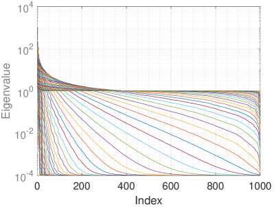
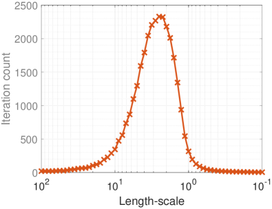
Figure 1: Left: Spectrum of $61$ regularized Gaussian kernel matrices associated with the same $1000$ points sampled randomly over a cube with edge length $10$ and a fixed regularization parameter $\mu=0.0001$ but different length-scales $l$. Right: Iteration counts of unpreconditioned CG to solve (1) for the $61$ regularized kernel matrices to reach the relative residual tolerance $10^{-4}$.

In this paper, we seek a preconditioner for kernel matrix systems (1) that is adaptive to different kernel matrices $\mathbf{K}$ corresponding to different values of kernel function parameters. When the numerical rank of $\mathbf{K}$ is small, there exist good methods [34, 16] for preconditioning $\mathbf{K}+\mu\mathbf{I}$ based on a Nyström approximation [38] to the kernel matrix. We will provide a detailed description of the Nyström approximation and the notation we will use, as it is related to our proposed preconditioner.

The $n\times n$ kernel matrix is defined by a kernel function and the set of $n$ training points $X=\{\mathbf{x}_{i}\}_{i=1}^{n}$. The Nyström approximation, which is inspired by solving an integral operator eigenvalue problem using the Nyström method, gives the low rank factorization

(3) $$\mathbf{K}\approx\widetilde{\mathbf{U}}\mathbf{\Lambda}\widetilde{\mathbf{U}}^{\top}$$

where $\mathbf{\Lambda}$ is a diagonal matrix of eigenvalues of the smaller $k\times k$ kernel matrix $\mathbf{K}_{X_{k},X_{k}}=[\mathcal{K}(x,y)]_{{x\in X_{k},\,y\in X_{k}}}$, $X_{k}=\{\mathbf{x}_{k_{i}}\}_{i=1}^{k}$ is a subset of $X$ consisting of $k$ data points referred to as landmark points. Additionally, $X_{k-1}$ is a subset of $X_{k}$. The $n\times k$ matrix $\widetilde{\mathbf{U}}$ does not have orthonormal columns, but the columns are Nyström extensions of the eigenvectors of $\mathbf{K}_{X_{k},X_{k}}$. The preconditioning operation that approximates the inverse of $\mathbf{K}+\mu\mathbf{I}$ utilizes the Sherman–Morrison–Woodbury (SMW) formula,

(4) $$(\widetilde{\mathbf{U}}\mathbf{\Lambda}\widetilde{\mathbf{U}}^{\top}+\mu\mathbf{I})^{-1}=\frac{1}{\mu}\mathbf{I}-\frac{1}{\mu}\widetilde{\mathbf{U}}(\mu\mathbf{\Lambda}^{-1}+\widetilde{\mathbf{U}}^{\top}\widetilde{\mathbf{U}})^{-1}\widetilde{\mathbf{U}}^{\top}.$$

Randomized Nyström approximations based on random projections [24, 34, 16] are often of the form

(5) $$\mathbf{K}\approx\mathbf{U}\widehat{\mathbf{\Lambda}}\mathbf{U}^{\top}$$

where $\mathbf{U}$ has explicitly orthonormalized columns and $\widehat{\mathbf{\Lambda}}$ is a diagonal matrix. Now utilizing the SMW formula and orthonormality, we have the simpler expression for the preconditioning operation:

(6) $$(\mathbf{U}\widehat{\mathbf{\Lambda}}\mathbf{U}^{\top}+\mu\mathbf{I})^{-1}=\mathbf{U}(\mathbf{\widehat{\Lambda}}+\mu\mathbf{I})^{-1}\mathbf{U}^{\top}+\frac{1}{\mu}(\mathbf{I}-\mathbf{U}\mathbf{U}^{\top}).$$

The randomized Nyström approximation based on random projections may be cheaper to compute if it is expensive to choose the landmark points (e.g., via computing leverage scores [10]). However, in some applications such as KRR, the original Nyström approximation appears to be more effective [16].

The above preconditioners using Nyström approximations and other low-rank approximations to the kernel matrix $\mathbf{K}$ involve at least an eigendecomposition or other factorization of a dense $k\times k$ matrix. These methods are effective for small $k$, but are costly for large $k$. In this paper, we address the case where the numerical rank of the kernel matrix is not small. In Section 2, we propose a 2-by-2 block approximate factorization of $\mathbf{K}+\mu\mathbf{I}$ as a preconditioner, where the (1,1) block corresponds to a set of landmark points. To select the landmark points for our preconditioner, we use farthest point sampling, and support this choice with an analysis in Section 3. We also propose a method for selecting the number of landmark points in Section 4. Section 5 demonstrates the effectiveness of the new preconditioner, and Section 6 summarizes the contributions of this paper.

2 Adaptive Factorized Nyström preconditioner

Let ${\mathbf{K}}_{nys}=\widetilde{\mathbf{U}}\mathbf{\Lambda}\widetilde{\mathbf{U}}^{\top}$ denote the Nyström approximation (3). The approximation is mathematically equal to [38]

(7) $${\mathbf{K}}_{nys}=\mathbf{K}_{X,X_{k}}\mathbf{K}_{X_{k},X_{k}}^{-1}\mathbf{K}_{X_{k},X}$$

where the notation was defined in the previous section. Without loss of generality, if the landmark points are indexed first, we can partition $\mathbf{K}$ into the block 2-by-2 form

(8) $$\mathbf{K}=\begin{bmatrix}\mathbf{K}_{11}&\mathbf{K}_{12}\\ \mathbf{K}_{12}^{\top}&\mathbf{K}_{22}\end{bmatrix},$$

where $\mathbf{K}_{11}=\mathbf{K}_{X_{k},X_{k}}$, $\mathbf{K}_{12}=\mathbf{K}_{X_{k},{X}\backslash X_{k}}$ and $\mathbf{K}_{22}=\mathbf{K}_{{X}\backslash X_{k},{X}\backslash X_{k}}$. In this notation,

(9) $${\mathbf{K}}_{nys}=\begin{bmatrix}\mathbf{K}_{11}&\mathbf{K}_{12}\\ \mathbf{K}_{12}^{\top}&\mathbf{K}_{12}^{\top}\mathbf{K}_{11}^{-1}\mathbf{K}_{12}\end{bmatrix}.$$

The difference $\mathbf{K}-{\mathbf{K}}_{nys}$ is positive semidefinite.

The Nyström preconditioner for $\mathbf{K}+\mu\mathbf{I}$ is ${\mathbf{K}}_{nys}+\mu\mathbf{I}$. For ${\mathbf{K}}_{nys}$ in the above form, solving with the Nyström preconditioner via the SMW formula requires applying the operator

(10) $$({\mathbf{K}}_{nys}+\mu\mathbf{I})^{-1}=\frac{1}{\mu}\mathbf{I}-\frac{1}{\mu^{2}}\begin{bmatrix}\mathbf{K}_{11}&\mathbf{K}_{12}\\ \end{bmatrix}^{\top}(\mathbf{K}_{11}+\frac{1}{\mu}(\mathbf{K}_{11}^{2}+\mathbf{K}_{12}\mathbf{K}_{12}^{\top}))^{-1}\begin{bmatrix}\mathbf{K}_{11}&\mathbf{K}_{12}\\ \end{bmatrix}$$

to a vector. The matrix $(\mathbf{K}_{11}+\frac{1}{\mu}(\mathbf{K}_{11}^{2}+\mathbf{K}_{12}\mathbf{K}_{12}^{\top}))$ is often ill-conditioned, but the ill-conditioning can be ameliorated [34] if the matrix is not too large (i.e., $k$ is not too large) and the Cholesky factorization of $\mathbf{K}_{11}$ can be computed rapidly.

We now propose a new preconditioner for $\mathbf{K}+\mu\mathbf{I}$ that can be efficient when $k$ is large. Recall that $\mathbf{K}_{11}$ is the kernel matrix associated with a set of landmark points $X_{k}$. In order to control the computational cost, we impose a limit on the maximum size of $X_{k}$ setting it to a constant value, such as $2000$. Let $\mathbf{LL^{\top}}$ be the Cholesky factorization of $\mathbf{K}_{11}+\mu\mathbf{I}$ and $\mathbf{G^{\top}G}$ be an approximate factorization of $(\mathbf{K}_{22}+\mu\mathbf{I}-\mathbf{K}_{12}^{\top}(\mathbf{K}_{11}+\mu\mathbf{I})^{-1}\mathbf{K}_{12})^{-1}$. Then we can define the following factorized preconditioner for $\mathbf{K}+\mu\mathbf{I}$:

(11) $$\mathbf{M}=\begin{bmatrix}\mathbf{L}&\mathbf{0}\\ \mathbf{K}_{12}^{\top}\mathbf{L}^{-\top}&\mathbf{G}^{-1}\end{bmatrix}\begin{bmatrix}\mathbf{L}^{\top}&\mathbf{L}^{-1}\mathbf{K}_{12}\\ \mathbf{0}&\mathbf{G}^{-\top}\end{bmatrix}.$$

Expanding the factors,

(12) $$\mathbf{M} =\begin{bmatrix}\mathbf{K}_{11}+\mu\mathbf{I}&\mathbf{K}_{12}\\ \mathbf{K}_{12}^{\top}&(\mathbf{G}^{\top}\mathbf{G})^{-1}+\mathbf{K}_{12}^{\top}(\mathbf{K}_{11}+\mu\mathbf{I})^{-1}\mathbf{K}_{12}\end{bmatrix}$$

(13) $$={\mathbf{K}}_{nys}+\mu\mathbf{I}+\underbrace{\begin{bmatrix}\mathbf{0}&\mathbf{0}\\ \mathbf{0}&(\mathbf{G}^{\top}\mathbf{G})^{-1}+\mathbf{K}_{12}^{\top}\left((\mathbf{K}_{11}+\mu\mathbf{I})^{-1}-(\mathbf{K}_{11})^{-1}\right)\mathbf{K}_{12}-\mu\,\mathbf{I}\end{bmatrix}}_{\text{Correction term}},$$

we see that $\mathbf{M}$ equals ${\mathbf{K}}_{nys}+\mu\mathbf{I}$ plus a correction term. Thus the preconditioner is not a Nyström preconditioner, but has similarities to it. Unlike a Nyström preconditioner, the factorized form approximates $\mathbf{K}+\mu\mathbf{I}$ entirely and does not approximate $\mathbf{K}$ separately, and thus avoids the SMW formula. In particular, when we have $\mathbf{G^{\top}G}=(\mathbf{K}_{22}+\mu\,\mathbf{I}-\mathbf{K}_{12}^{\top}(\mathbf{K}_{11}+\mu\,\mathbf{I})^{-1}\mathbf{K}_{12})^{-1}$ exactly, $\mathbf{M}=\mathbf{K}+\mu\,\mathbf{I}$.

The preconditioner requires an economical way to approximately factor the generally dense matrix $(\mathbf{K}_{22}+\mu\,\mathbf{I}-\mathbf{K}_{21}(\mathbf{K}_{11}+\mu\,\mathbf{I})^{-1}\mathbf{K}_{12})^{-1}$, which can be large. For this, we use the factorized sparse approximate inverse (FSAI) method of Kolotilina and Yeremin [22]. We use FSAI to compute a sparse approximate inverse $\mathbf{G}$ of the lower triangular Cholesky factor of a symmetric positive definite (SPD) matrix $\mathbf{K}_{22}+\mu\,\mathbf{I}-\mathbf{K}_{21}(\mathbf{K}_{11}+\mu\,\mathbf{I})^{-1}\mathbf{K}_{12}$, given a sparsity pattern for $\mathbf{G}$, i.e., $\mathbf{G^{\top}G}\approx(\mathbf{K}_{22}+\mu\,\mathbf{I}-\mathbf{K}_{21}(\mathbf{K}_{11}+\mu\,\mathbf{I})^{-1}\mathbf{K}_{12})^{-1}$. An important feature of FSAI is that the computation of $\mathbf{G}$ only requires the entries of $\mathbf{K}_{22}+\mu\,\mathbf{I}-\mathbf{K}_{21}(\mathbf{K}_{11}+\mu\,\mathbf{I})^{-1}\mathbf{K}_{12}$ corresponding to the sparsity pattern of $\mathbf{G}$ and $\mathbf{G}^{\top}$. This makes it possible to economically compute $\mathbf{G}$ even if $\mathbf{K}_{22}+\mu\,\mathbf{I}-\mathbf{K}_{21}(\mathbf{K}_{11}+\mu\,\mathbf{I})^{-1}\mathbf{K}_{12}$ is large and dense. Further, the computation of each row of $\mathbf{G}$ is independent of other rows and is thus the rows of $\mathbf{G}$ can be computed in parallel. The nonzero pattern used for row $i$ of $\mathbf{G}$ corresponds to the $w-1$ nearest neighbors of point $i$ that are numbered less than $i$ (since $\mathbf{G}$ is lower triangular), where $w$ is a parameter.

The preconditioning operation for this proposed Adaptive Factorized Nyström (AFN) preconditioner solves systems with the matrix $\mathbf{M}$. Assuming that the vectors $\mathbf{r}$ and $\mathbf{s}$ are partitioned conformally with the block structure of $\mathbf{M}$, then to solve the system

$$\mathbf{M}\begin{bmatrix}\mathbf{s}_{1}\\ \mathbf{s}_{2}\end{bmatrix}=\begin{bmatrix}\mathbf{r}_{1}\\ \mathbf{r}_{2}\end{bmatrix},$$

the algorithm is

$$\mathbf{s}_{2} :=\mathbf{G}^{\top}\mathbf{G}\left(\mathbf{r}_{2}-\mathbf{K}_{12}^{\top}(\mathbf{L}^{-\top}\mathbf{L}^{-1})\mathbf{r}_{1}\right),$$

$$\mathbf{s}_{1} :=\mathbf{L}^{-\top}\mathbf{L}^{-1}(\mathbf{r}_{1}-\mathbf{K}_{12}\mathbf{s}_{2}).$$

In the algorithm, the multiplications by $\mathbf{K}_{12}$ and $\mathbf{K}_{12}^{\top}$, can be performed rapidly using hierarchical matrix methods.

The choice of the landmark points affects the accuracy of the overall AFN preconditioner, just as this choice affects the accuracy of the Nyström preconditioners. The sparsity and the conditioning of $\mathbf{K}_{22}+\mu\,\mathbf{I}-\mathbf{K}_{12}^{\top}(\mathbf{K}_{11}+\mu\,\mathbf{I})^{-1}\mathbf{K}_{12}$ generally improves when more landmark points are chosen, which would on the other hand increase the computational cost and the instability of the Cholesky factorization of $\mathbf{K}_{11}+\mu\mathbf{I}$. In the next section, the choice of landmark points is discussed in light of these considerations.

3 Selecting the landmark points

Existing methods for selecting landmark points include uniform sampling [38], the anchor net method [6, 8], leverage score sampling [11, 17, 25], $k$-means-based sampling [40], and determinantal point process (DPP)-based sampling [3]. For our proposed preconditioner, we will select the landmark points based on a trade-off between two geometric measures in order to make the preconditioner effective and robust.

The first measure $h_{X_{k}}$, called fill distance [15, 23], is used to quantify how well the points in $X_{k}$ fill out a domain $\Omega$:

(14) $$h_{X_{k}}=\max_{\mathbf{x}\in\Omega\backslash X_{k}}\operatorname{dist}(\mathbf{x},X_{k}),$$

where $\operatorname{dist}(\mathbf{x},Y)=\inf_{\mathbf{y}\in Y}\|\mathbf{x}-\mathbf{y}\|$ is the distance between a point $\mathbf{x}$ and a set $Y$, and where $\Omega$ denotes the domain of the kernel function under consideration which can be either a continuous region or a finite discrete set. The geometric interpretation of this measure is the radius of an empty ball in $\Omega$ that does not intersect with $X_{k}$. This implies $X_{k}$ with a smaller fill distance will better fill out $\Omega$. Since $\mathbf{K}_{22}+\mu\,\mathbf{I}-\mathbf{K}_{12}^{\top}(\mathbf{K}_{11}+\mu\,\mathbf{I})^{-1}\mathbf{K}_{12}$ can be considered as the conditional covariance matrix of $X\backslash X_{k}$ conditioned on $X_{k}$ [33, 32], the screening effect [20, 28] implies that a smaller $h_{X_{k}}$ often yields a $\mathbf{K}_{22}+\mu\,\mathbf{I}-\mathbf{K}_{12}^{\top}(\mathbf{K}_{11}+\mu\,\mathbf{I})^{-1}\mathbf{K}_{12}$ that has more entries with small magnitude.

The second measure $q_{X_{k}}$, called separation distance [15, 23], is defined as the distance between the closest pair of points in $X_{k}$:

(15) $$q_{X_{k}}=\min_{\mathbf{x}_{k_{i}},\mathbf{x}_{k_{j}}\in X_{k},k_{i}\neq k_{j}}\operatorname{dist}(\mathbf{x}_{k_{i}},\mathbf{x}_{k_{j}}).$$

The geometric interpretation of this measure is the diameter of the largest ball that can be placed around every point in $X_{k}$ such that no two balls overlap. A larger $q_{X_{k}}$ indicates that the columns in $\mathbf{K}_{11}$ tend to be more linearly independent and thus leads to a more well-conditioned $\mathbf{K}_{11}$. The conditioning of $\mathbf{K}_{11}$ will affect the numerical stability of $\mathbf{L}$.

As more landmark points are sampled, both $h_{X_{k}}$ and $q_{X_{k}}$ tend to decrease. We wish to choose $X_{k}$ such that $h_{X_{k}}$ is small while $q_{X_{k}}$ is large. We will analyze the interplay between $h_{X_{k}}$ and $q_{X_{k}}$ in Section 3.1. In particular, we will show that if $h_{X_{k}}\leq Cq_{X_{k}}$ for some constant $C$, then $h_{X_{k}}$ and $q_{X_{k}}$ have the same order as the minimal value of the fill distance and the maximal value of the separation distance that can be achieved with $k$ points, respectively.

Moreover, we find that Farthest Point Sampling (FPS) [13] can generate landmark points with $h_{X_{k}}\leq q_{X_{k}}$. FPS is often used in mesh generation [27] and computer graphics [31]. In spatial statistics, FPS is also known as MaxMin Ordering (MMD) [20]. FPS initializes $X_{1}$ with an arbitrary point $\mathbf{x}_{k_{1}}$ in $X$ (better choices are possible). At step $i+1$, FPS selects the point that is farthest away from $X_{i}$

(16) $$\mathbf{x}_{k_{i+1}}=\operatorname*{arg\,max}_{\mathbf{x}\in X\backslash X_{i}}\operatorname{dist}(\mathbf{x},X_{i}).$$

See Figure 2 for an illustration of FPS on a two-dimensional dataset.

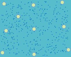
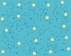
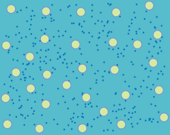
Figure 2: An illustration of FPS for selecting one, ten, twenty and thirty points from a two-dimensional dataset with $400$ points where the big circles represent the selected points and the dots denote the other data points.

The landmark points selected by FPS spread evenly in the dataset and do not form dense clusters. We will justify the use of FPS to select landmark points in the construction of the AFN preconditioner in Section 3.2.

3.1 Interplay between fill and separation distance

In this section, we will study the relationship between $h_{X_{k}}$ and $q_{X_{k}}$. We will show that if $h_{X_{k}}\leq Cq_{X_{k}}$ for a constant $C$, then $h_{X_{k}}$ and $q_{X_{k}}$ will have the same order as the minimal fill distance and maximal separation distance that can be achieved with any subset with $k$ points, respectively.

First notice that there exist a lower bound for $h_{X_{k}}$ and a upper bound for $q_{X_{k}}$, which is analyzed in the next theorem when all the points are inside a unit ball in $\mathbb{R}^{d}$.

Theorem 3.1.

Suppose all the data points are inside a unit ball $\Omega$ in $\mathbb{R}^{d}$. Then for an arbitrary subset $X_{k}=\{\mathbf{x}_{i_{1}},\dots,\mathbf{x}_{i_{k}}\}$ of $X$, the following bounds hold for $h_{X_{k}}$ and $q_{X_{k}}$:

(17) $$h_{X_{k}}\geq C_{\Omega}k^{-1/d}\quad\text{and} \quad q_{X_{k}}\leq C_{\Omega}^{\prime}k^{-1/d},$$

where $C_{\Omega}$ and $C^{{}^{\prime}}_{\Omega}$ are two constants only depending on $\Omega$.

Proof 3.2.

In order to show the lower bound of $h_{X_{k}}$, we first derive an upper bound of the volume of $\Omega$. Notice that $\Omega\subset\bigcup_{i=1}^{k}B_{h_{X_{k}}}(\mathbf{x}_{k_{i}})$ where $B_{h_{X_{k}}}(\mathbf{x}_{k_{i}})$ is the ball centered at $\mathbf{x}_{k_{i}}$ with radius $h_{X_{k}}$. Then

$$\text{Vol}(\Omega) \leq\sum_{i=1}^{k}\text{Vol}(B_{h_{X_{k}}}(\mathbf{x}_{k_{i}}))=k\frac{\pi^{d/2}}{\Gamma(\frac{d}{2}+1)}h_{X_{k}}^{d}.$$

Setting $C_{\Omega}:=1$ gives us the first bound.

Similarly, we get an upper bound of $q_{X_{k}}$ by deriving a lower bound of the volume of $\Omega$:

$$\text{Vol}(\Omega) \geq\text{Vol}(\Omega\bigcap\bigcup_{i=1}^{k}B_{\frac{q_{X_{k}}}{2}}(\mathbf{x}_{k_{i}}))=\sum_{i=1}^{k}\text{Vol}(\Omega\bigcap B_{\frac{q_{X_{k}}}{2}}(\mathbf{x}_{k_{i}}))$$

$$\geq\frac{1}{2}\sum_{i=1}^{k}\text{Vol}(B_{\frac{q_{X_{k}}}{2}}(\mathbf{x}_{k_{i}}))=k\frac{\pi^{d/2}}{2^{d+1}\Gamma(\frac{d}{2}+1)}q_{X_{k}}^{d}.$$

Here we use the fact that Vol$(\Omega\bigcap B_{\frac{q_{X_{k}}}{2}}(\mathbf{x}_{k_{i}}))\geq\frac{\pi}{2\pi}\text{Vol}(B_{\frac{q_{X_{k}}}{2}}(\mathbf{x}_{k_{i}}))$. Then setting $C^{{}^{\prime}}_{\Omega}:=2^{\frac{d+1}{d}}$ gives us the second bound.

Remark 3.3.

Similar bounds can be derived for more complex bounded domains $\Omega$ that satisfy the interior cone condition [26].

The bounds in Theorem 3.1 say that the minimal fill distance $h_{X_{k}}$ cannot be smaller than $C_{\Omega}k^{-1/d}$ while the maximal separation distance $q_{X_{k}}$ cannot be greater than $C_{\Omega}^{{}^{\prime}}k^{-1/d}$ and $\frac{C_{\Omega}}{C_{\Omega}^{{}^{\prime}}}q_{X_{k}}\leq h_{X_{k}}$. In the following theorem, we show that if a sampling scheme can select a subset $X_{k}$ with $h_{X_{k}}\leq Cq_{X_{k}}$, then $q_{X_{k}}$ has the same order as the maximal separation distance that can be achieved by a subset with $k$ points.

Theorem 3.4.

Assume the data points are on a bounded domain $\Omega$ that satisfies the interior cone condition, then if $h_{X_{k}}\leq Cq_{X_{k}}$

(18) $$C_{\Omega}k^{-1/d}\leq h_{X_{k}}\leq C\times C_{\Omega}^{\prime}k^{-1/d}, \quad\frac{C_{\Omega}}{C}k^{-1/d}\leq q_{X_{k}}\leq C_{\Omega}^{\prime}k^{-1/d}.$$

Proof 3.5.

If $h_{X}\leq Cq_{X}$, then Theorem 3.1 yields

$$C_{\Omega}k^{-1/d}\leq h_{X_{k}}\leq Cq_{X_{k}}\leq C\times C_{\Omega}^{\prime}k^{-1/d}.$$

Theorem 3.4 shows that $h_{X_{k}}$ is at most $C\times\frac{C^{{}^{\prime}}_{\Omega}}{C_{\Omega}}$ times larger than its theoretical lower bound and $q_{X_{k}}$ is at least $\frac{1}{C}\times\frac{C_{\Omega}}{C_{\Omega^{{}^{\prime}}}}$ times as large as its theoretical upper bound in this case.

3.2 Farthest point sampling

In this section, we justify the use of FPS in the construction of the proposed preconditioner. FPS is a greedy algorithm designed to select a set of data points with maximal dispersion at each iteration. FPS can generate $X_{k}$ with $h_{X_{k}}$ at most $2$ times the minimal fill distance [18] and $q_{X_{k}}$ at least half the largest separation distance over all subsets with $k$ points [37]. In the next theorem, we first verify that FPS can generate $X_{k}$ with $h_{X_{k}}\leq q_{X_{k}}$ and then use this result to show these two near-optimality properties in a unified way.

Theorem 3.6.

Suppose the minimal fill distance of a subset with $k$ points is achieved with $X^{\ast}_{k}$ and the maximal separation distance of a subset with $k$ points is achieved with $X_{k\ast}$. Then the set $X_{k}$ sampled by FPS satisfies

(19) $$h_{X_{k}}\leq q_{X_{k}}\quad\text{and}\quad q_{X_{k}}\geq\frac{1}{2}q_{X_{k*}}\quad\text{and}\quad h_{X_{k}}\leq 2h_{X_{k}^{\ast}}.$$

Proof 3.7.

Without loss of generality, we assume the subset $X_{k}$ sampled by FPS contains the points $\mathbf{x}_{1},\mathbf{x}_{2},\ldots,\mathbf{x}_{k}$. Suppose $q_{X_{k}}=\operatorname{dist}(\mathbf{x}_{j},\mathbf{x}_{m})$ with $j<m<(k+1)$, and point $\mathbf{x}_{m}$ is selected at iteration $m$ by FPS, then

(20) $$h_{X_{m-1}}=\max_{\mathbf{x}\in X\backslash X_{m-1}}\operatorname{dist}(\mathbf{x},X_{m-1})=\operatorname{dist}(\mathbf{x}_{j},\mathbf{x}_{m})=q_{X_{k}}.$$

Since $h_{X_{k}}$ is a non-increasing function of $k$, we have $h_{X_{k}}\leq h_{X_{m-1}}=q_{X_{k}}$.

We now prove $q_{X_{k}}\geq\frac{1}{2}q_{X_{k}*}$. According to the definition, there exists a subset with $k$ points $X_{k*}=\{\mathbf{x}^{1}_{*},\dots,\mathbf{x}^{k}_{*}\}$ such that

$$q_{X_{k*}}=\max_{Y\subset X,|Y|=k}\;\min_{\mathbf{x}_{i},\mathbf{x}_{j}\in Y}\operatorname{dist}(\mathbf{x}_{i},\mathbf{x}_{j}).$$

According to (20), we know all the points in $X$ must lie in one of the $m-1$ disks defined by

(21) $$C(\mathbf{x}_{i},q_{X_{k}})=\{\mathbf{x}|\|\mathbf{x}-\mathbf{x}_{i}\|\leq q_{X_{k}}\},\quad i\in[m-1].$$

Since $m-1<k$, at least two points $\mathbf{x}^{i}_{*},\mathbf{x}^{j}_{*}\in X_{k*}$ must belong to the same disk centered at some $\mathbf{x}_{l}$. Therefore, $2q_{X_{k}}\geq\operatorname{dist}(\mathbf{x}^{i}_{*},\mathbf{x}_{l})+\operatorname{dist}(\mathbf{x}^{j}_{*},\mathbf{x}_{l})\geq\operatorname{dist}(\mathbf{x}^{i}_{*},\mathbf{x}^{j}_{*})\geq q_{X_{k}*}$ via the triangle inequality.

Next, we prove $h_{X_{k}}\leq 2h_{X_{k}^{\ast}}$. At the $k$th iteration of FPS, the set $X$ can be split into $k$ clusters $\{C_{i}\}_{i=1}^{k}$ such that the point $\mathbf{x}$ in $X$ will be classified into cluster $C_{i}$ if $\operatorname{dist}(\mathbf{x}_{i},\mathbf{x})\leq\operatorname{dist}(\mathbf{x}_{j},\mathbf{x}),~{}\forall j\neq i$. At the $(k+1)$th iteration of FPS, one more point $\mathbf{x}_{k+1}$ will be selected. Then we can show that

$$\operatorname{dist}(\mathbf{x}_{i},\mathbf{x}_{j})\geq h_{X_{k}}\quad\text{for}\quad i,j\in\{1,2,\ldots,k+1\},$$

and in particular

$$q_{X_{k+1}}\geq h_{X_{k}}.$$

Assume $\mathbf{x}_{k+1}\in C_{i}$. From the definition of $h_{X_{k}}$, we know that $\operatorname{dist}(\mathbf{x}_{k+1},\mathbf{x}_{i})=h_{X_{k}}$ and $\operatorname{dist}(\mathbf{x}_{k+1},\mathbf{x}_{j})\geq\operatorname{dist}(\mathbf{x}_{k+1},\mathbf{x}_{i})$ for $j\neq i$. Moreover, we have $\operatorname{dist}(\mathbf{x}_{i},\mathbf{x}_{j})\geq q_{X_{k}}$ for $j\neq k+1$. Since $q_{X_{k}}\geq h_{X_{k}}$, we know $q_{X_{k+1}}=\operatorname{dist}(\mathbf{x}_{i},\mathbf{x}_{j})\geq h_{X_{k}}$.

Finally, assume $\mathbf{x}^{\ast}_{1},\mathbf{x}^{\ast}_{2},\ldots,\mathbf{x}^{\ast}_{k}$ are the optimal subset of $X$ that achieves the minimal fill distance with cardinality $k$. Now the set $X$ can be split into $k$ clusters $\{{C}^{\ast}_{i}\}_{i=1}^{k}$ such that the point $\mathbf{x}$ in $X$ will be classified into $C^{\ast}_{i}$ if $\operatorname{dist}(\mathbf{x}_{i}^{\ast},\mathbf{x})\leq\operatorname{dist}(\mathbf{x}_{j}^{\ast},\mathbf{x}),~{}\forall j\neq i$. Assume the points selected by FPS in the first $k+1$ iterations are $\mathbf{x}_{1},\mathbf{x}_{2},\ldots,\mathbf{x}_{k+1}$. We know that at least two points from $\mathbf{x}_{1},\mathbf{x}_{2},\ldots,\mathbf{x}_{k+1}$ belong to the same cluster. Denote these two points as $\mathbf{x}_{p}$ and $\mathbf{x}_{q}$ and the corresponding cluster is $C^{\ast}_{j}$. Then we have

$$h_{X_{k}}\leq q_{X_{k+1}}\leq\operatorname{dist}(\mathbf{x}_{p},\mathbf{x}_{q})\leq\operatorname{dist}(\mathbf{x}_{p},\mathbf{x}^{\ast}_{i})+\operatorname{dist}(\mathbf{x}_{q},\mathbf{x}^{\ast}_{i})\leq 2h_{X^{\ast}_{k}},$$

which indicates that $h_{X_{k}}\leq 2h_{X^{\ast}_{k}}$.

We now demonstrate the screening effect (mentioned in Section 3) numerically with an example in Figure 3 when FPS is applied to select landmark points. Figure 3 shows histograms of the magnitude of the entries in three matrices $\mathbf{K}_{22}+\mu\mathbf{I}$, $\mathbf{K}_{22}+\mu\,\mathbf{I}-\mathbf{K}_{12}^{\top}(\mathbf{K}_{11}+\mu\,\mathbf{I})^{-1}\mathbf{K}_{12}$ and $(\mathbf{K}_{22}+\mu\,\mathbf{I}-\mathbf{K}_{12}^{\top}(\mathbf{K}_{11}+\mu\,\mathbf{I})^{-1}\mathbf{K}_{12})^{-1}$ for $l=5$, with the matrices scaled so that their maximum entries are equal to one. The $1000$ data points $X$ are generated uniformly over a cube with edge length $10$ and $100$ landmark points $X_{100}$ are selected by FPS. The figure shows that $\mathbf{K}_{22}+\mu\,\mathbf{I}-\mathbf{K}_{12}^{\top}(\mathbf{K}_{11}+\mu\,\mathbf{I})^{-1}\mathbf{K}_{12}$ and its inverse have many more entries with smaller magnitude than $\mathbf{K}_{22}+\mu\mathbf{I}$. This example further justifies that $(\mathbf{K}_{22}+\mu\,\mathbf{I}-\mathbf{K}_{12}^{\top}(\mathbf{K}_{11}+\mu\,\mathbf{I})^{-1}\mathbf{K}_{12})^{-1}$ has more “sparsity” than $\mathbf{K}_{22}+\mu\,\mathbf{I}-\mathbf{K}_{12}^{\top}(\mathbf{K}_{11}+\mu\,\mathbf{I})^{-1}\mathbf{K}_{12}$, which supports the use of FSAI.

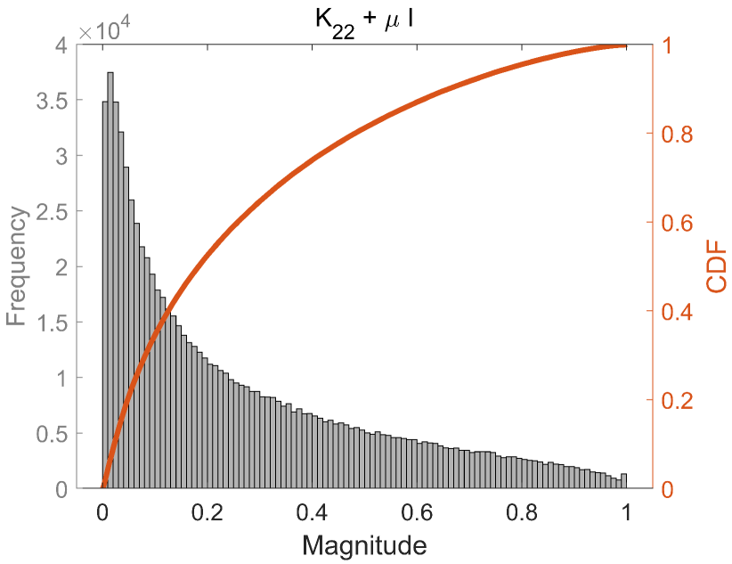
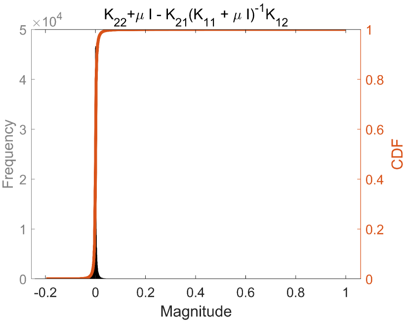
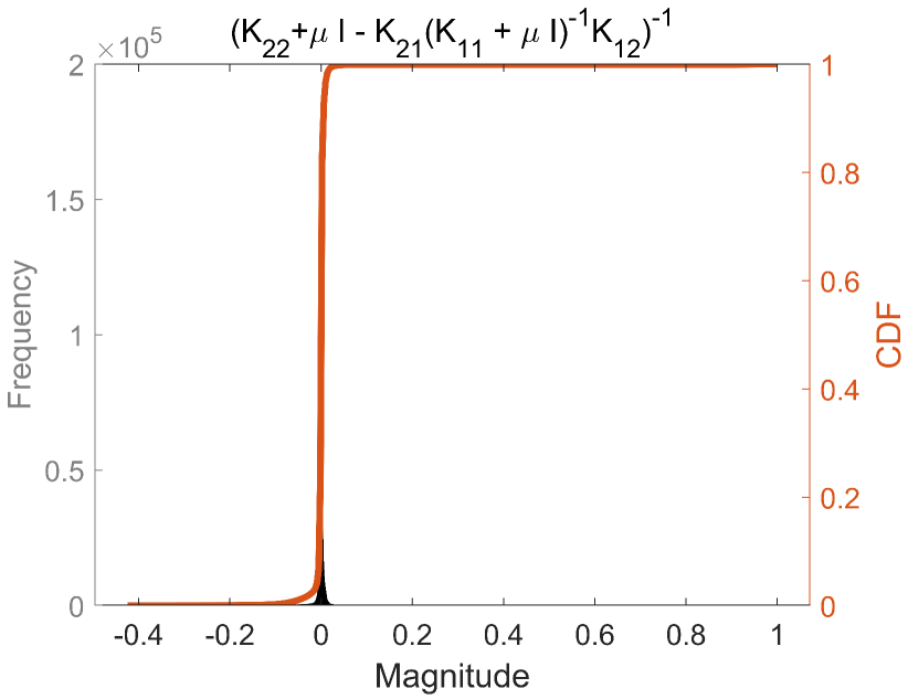
Figure 3: Histograms of the magnitude of the entries in $\mathbf{K}_{22}+\mu\mathbf{I}$, $\mathbf{K}_{22}+\mu\,\mathbf{I}-\mathbf{K}_{12}^{\top}(\mathbf{K}_{11}+\mu\,\mathbf{I})^{-1}\mathbf{K}_{12}$, and $(\mathbf{K}_{22}+\mu\,\mathbf{I}-\mathbf{K}_{12}^{\top}(\mathbf{K}_{11}+\mu\,\mathbf{I})^{-1}\mathbf{K}_{12})^{-1}$ associated with a Gaussian kernel matrix defined using $1000$ points sampled uniformly from a cube with edge length $10$, regularization parameter $\mu=0.0001$, and length-scale $l=5$. The maximum entries in these three matrices are all scaled to $1$. $\mathbf{K}$ has $243$ eigenvalues greater than $1.1\times\mu$.

3.3 Implementation of FPS

A naive implementation of FPS for selecting $k$ samples from $n$ points in $\mathbb{R}^{d}$ scales as $O(dk^{2}n)$. The scaling can be reduced to $O(\rho^{d}n\log n)$ by using an algorithm [33] that keeps the distance information in a heap and that only updates part of the heap when a new point is added to the set $X_{k}$. Here, $\rho$ is a constant greater than $1$ that controls the efficiency the sampling process.

4 Adaptive choice of approximation rank

In order to construct a preconditioner that is adaptive and efficient for a range of regularized kernel matrices arising from different values of the kernel function parameters, it is necessary to estimate the rank of the kernel matrix $\mathbf{K}$. For example, if the estimated rank is small enough that it is inexpensive to perform an eigendecomposition of a $k$-by-$k$ matrix, then the Nyström preconditioner should be used due to the reduced construction cost.

4.1 Nyström approximation error analysis based on fill distance

Define the Nyström approximation error as

$$\|\mathbf{K}-{\mathbf{K}}_{nys}\|=\|\mathbf{K}_{22}-\mathbf{K}_{21}\mathbf{K}_{11}^{-1}\mathbf{K}_{12}\|.$$

In this section, we will show that the Nyström approximation error is also related to the fill distance $h_{X_{k}}$. In particular, for Gaussian kernels defined in (2) and inverse multiquadric kernels

(22) $$\mathcal{K}(\mathbf{x},\mathbf{y})=(c^{2}+\|\mathbf{x}-\mathbf{y}\|^{2})^{-\frac{p}{2}},~{}p>0,~{}c\in\mathbb{R},$$

we can derive a Nyström approximation error estimate in terms of the fill distance, as presented in the following theorem.

Theorem 4.1.

The Nyström approximation ${\mathbf{K}}_{nys}=\mathbf{K}_{{X},X_{k}}\mathbf{K}_{X_{k},X_{k}}^{-1}\mathbf{K}_{X_{k},X}$ to $\mathbf{K}$ using the landmark points $X_{k}=\{\mathbf{x}_{k_{i}}\}_{i=1}^{k}$ has the following error estimate

(23) $$\|\mathbf{K}-{\mathbf{K}}_{nys}\|<\sqrt{n\|\mathbf{K}\|}C^{\prime}\exp(-C{{}^{\prime\prime}}/h_{X_{k}}),$$

where $C^{\prime}$ and $C{{}^{\prime\prime}}$ are constants independent of $X_{k}$.

The detailed proof of Theorem 4.1 is in Appendix A. Theorem 4.1 implies landmark points $X_{k}$ with a smaller fill distance can yield a more accurate Nyström approximation. We illustrate this numerically with an experiment. In Figure 4, we plot the fill distance curve and the Nyström approximation error curve corresponding to a Gaussian kernel with $l=10$ when $1000$ points are uniformly sampled from a cube with edge length $10$. We test random sampling and FPS for selecting the landmark points and observe that FPS leads to a smaller fill distance than random sampling. We also observe that FPS Nyström can achieve lower approximation errors than the randomly sampled one when the same $k$ is used. Thus we will use FPS to select landmark points in the construction of Nyström-type preconditioners if the estimated rank is small. Meanwhile, the rank estimation algorithm discussed in the next section also relies on FPS.

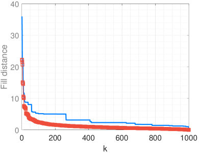
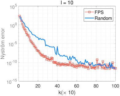
Figure 4: Comparison of fill distance and the Nyström approximation error for $1000$ points uniformly sampled from a cube with edge length $10$, when the Gaussian kernel function with length-scale $l=10$ is used. FPS and random sampling are used to sample $k$ points from $X$ to form $X_{k}$. Nyström error is computed only for the ranks which are multiples of $10$.

The error estimate in (4.1) does not involve the length-scale $l$ explicitly. However, this error estimate can still help understand how the length-scale in Gaussian kernels affects the Nyström approximation error when the same landmark points $X_{k}$ are used. Assume $h_{X_{k}}$ is the fill distance of $X_{k}$ associated with the unit length-scale. When we change the length-scale to $l$, the kernel matrix associated with length-scale $l$ can be regarded as a kernel matrix associated with the unit length-scale and the scaled data points $\tilde{\mathbf{x}}=\mathbf{x}/l$. This is because $\|\tilde{\mathbf{x}}-\tilde{\mathbf{y}}\|=\|\frac{\mathbf{x}}{l}-\frac{\mathbf{y}}{l}\|=\frac{1}{l}\operatorname{dist}(\mathbf{x},\mathbf{y})$. In this case, the fill distance on the rescaled data points becomes $\frac{h_{X_{k}}}{l}$. As a result, as $l$ increases, the exponential factor in the estimate decays faster. This is consistent with the fact that the Gaussian kernel matrix $\mathbf{K}$ is numerically low-rank when $l$ is large.

4.2 Nyström rank estimation based on subsampling

It is of course too costly in general to use a rank-revealing decomposition of $\mathbf{K}$ to compute $k$. Instead, we will compute $k$ that approximately achieves a certain Nyström approximation accuracy via checking the relative Nyström approximation error on a subsampled dataset.

First, a dataset $X_{m}$ of $m$ points is randomly subsampled from $X$. The number of points $m$ is an input to the procedure, and $m$ can be much smaller than the $k$ that will be computed. Then the coordinates of the data points in $X_{m}$ are scaled by $(m/n)^{1/d}$ and the smaller kernel matrix $\mathbf{K}_{X_{m},X_{m}}$ is formed. The rationale of this scaling is that we expect the spectrum of $\mathbf{K}_{X_{m},X_{m}}$ has a similar decay pattern as that of $\mathbf{K}_{X,X}$. We now run FPS on $X_{m}$ to construct Nyström approximations with increasing rank to $\mathbf{K}$ until the relative Nyström approximation error falls below $0.1$ and define this Nyström rank as $r$. Finally, we approximate the Nyström rank of $\mathbf{K}$ as $rn/m$. Figure 5 plots the Nyström approximation errors on subsampled matrices and original matrices associated with two different length-scales. The data points $X$ are generated randomly by sampling $1000$ points uniformly within a cube and $m=100$ points are subsampled randomly. The two relative Nyström approximation error curves show a close match in both cases. This rank estimation method is summarized in Algorithm 1. We also find that if the estimated rank is small (e.g., less than $2000$), we can perform an eigen-decomposition of $\mathbf{K}_{{X}_{m},{X}_{m}}$ associated with the unscaled data points and refine the estimation with the number of eigenvalues greater than $0.1$.

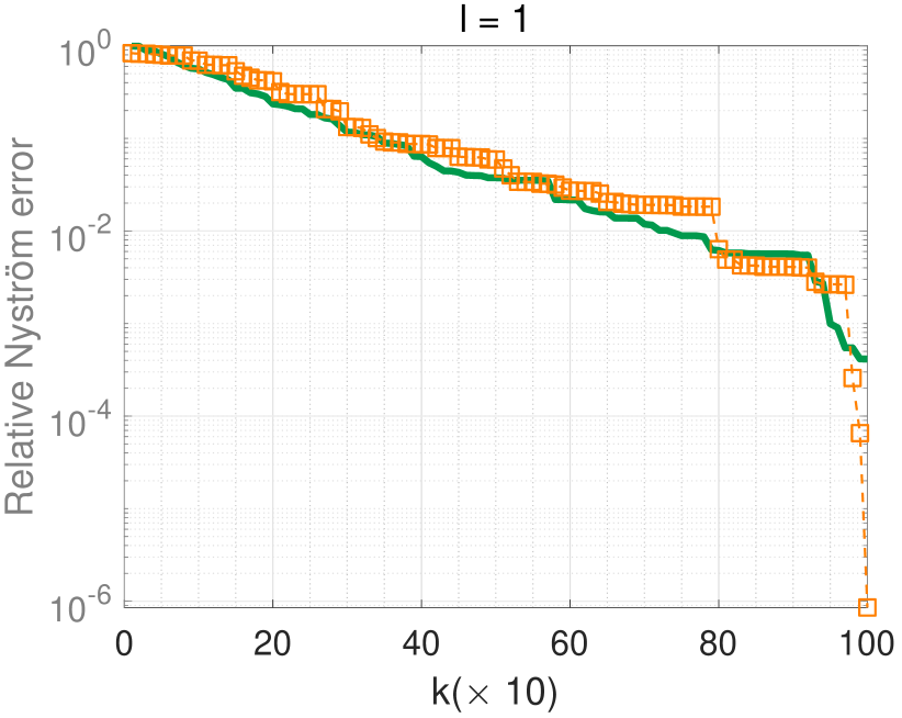
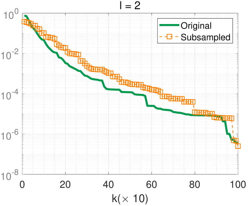
Figure 5: Comparison of the relative Nyström approximation error curves for an original dataset and a subsampled dataset with $100$ points, associated with two different length-scales. The original dataset contains 1000 uniformly sampled points from a cube with edge length $10$. The indices of the subsampled dataset are matched with those of the original dataset by computing the relative Nyström approximation errors on the original dataset only for ranks that are multiples of 10. The plot shows how the approximation error changes as the rank of the approximation increases.

Algorithm 1 Nyström rank estimation

1:  Input: dataset $X$ with size $n$, subsample size $m$, and kernel function $\mathcal{K}(\mathbf{x},\mathbf{y})$

2:  Output: approximate Nyström rank $k$

3:  Randomly subsample a subset $X_{m}$ of $m$ points from $X$ and scale the coordinates of $X_{m}$ by $({m}/{n})^{1/d}$

4:  Form the $m\times m$ matrix $\mathbf{K}_{{X}_{m},{X}_{m}}$

5:  Find the Nyström rank $r$ such that the relative Nyström approximation error for $\mathbf{K}_{{X}_{m},{X}_{m}}$ with FPS sampling falls below $0.1$

6:  Compute $k={rn}/{m}$

7:  if $k\geq 2000$ then

8:     Return $k={rn}/{m}$

9:  else

10:     Compute eigenvalues of $\mathbf{K}_{{X}_{m},{X}_{m}}$ associated with the unscaled data points

11:     Return $k=\#$ of eigenvalues greater than 0.1

12:  end if

If the estimated rank $k$ is smaller than $2000$, then the Nyström preconditioner should be used. AFN is only constructed when the estimated rank exceeds $2000$ for better efficiency. The selection of the preconditioning method is shown precisely in Algorithm 2.

Algorithm 2 Choosing the preconditioning method

1:  Input: dataset $X$, subsample size $m$

2:  Estimate numerical rank $k$ of $\mathbf{K}$ with Algorithm 1

3:  if $k\geq 2000$ then

4:     Use AFN preconditioner

5:  else

6:     Use Nyström preconditioner with $k$ landmark points selected by FPS

7:  end if

8:  Return

5 Numerical experiments

The AFN preconditioner and the preconditioning strategy (Algorithm 2) are tested for the iterative solution of regularized kernel matrix systems (1) over a wide range of length-scale parameters $l$ in the following two kernel functions

• Gaussian kernel: $\mathcal{K}(\mathbf{x},\mathbf{y})=\exp\left(-\frac{1}{l^{2}}\|\mathbf{x}-\mathbf{y}\|_{2}^{2}\right)$

• Matérn-3/2 kernel: $\mathcal{K}(\mathbf{x},\mathbf{y})=\left(1+\frac{\sqrt{3}}{l}||\mathbf{x}-\mathbf{y}||_{2}\right)\exp\left(-\frac{\sqrt{3}}{l}||\mathbf{x}-\mathbf{y}||_{2}\right)$.

We also benchmark the solution of these systems using unpreconditioned CG, and preconditioned CG, with the FSAI preconditioner and with the randomized Nyström (RAN) preconditioner [16] with randomly selected $k$ landmark points.

RAN approximates the kernel matrix with a rank-$k$ Nyström approximation based on randomly sampling the data points. Assuming the $k$-th largest eigenvalue of ${\mathbf{K}}_{nys}$ is $\lambda_{k}$, the inverse of the RAN preconditioner takes the form [16]: $(\lambda_{k}+\mu)\mathbf{U}(\mathbf{\Lambda}+\mu\mathbf{I})^{-1}\mathbf{U}^{\top}+(\mathbf{I}-\mathbf{U}\mathbf{U}^{\top})$ where $\mathbf{U}\mathbf{\Lambda}\mathbf{U}^{\top}$ is the eigendecomposition of ${\mathbf{K}}_{nys}$. In our experiments, we use $400$ nearest neighbors as the sparsity pattern for FSAI, fix the Nyström rank to be $3000$ for RAN, and use $100$ nearest neighbors as the sparsity pattern for the FSAI used in AFN.

The stopping tolerance for the relative residual norm is set to be $10^{-4}$. We randomly generated right-hand side vectors in Equation (1) with entries from the uniform distribution $[-0.5,0.5]$. For all tests we perform 3 runs and report the average results.

AFN, RAN and FSAI have been implemented in C. Experiments are run on an Ubuntu 20.04.4 LTS machine equipped with 755 GB of system memory and a 24-core 3.0 GHz Intel Xeon Gold 6248R CPU. We build our code with the GCC 9.4.0 compiler and take advantage of shared memory parallelism using OpenMP. We use the parallel BLAS and LAPACK implementation in the OpenBLAS library for basic matrix operations. H2Pack [7, 21] is used to provide linear complexity matrix-vector multiplications associated with large-scale $\mathbf{K}$ for 3D datasets with the relative error threshold $1e\!-\!8$. We utilized a brute force parallel FPS algorithm on the global dataset. OpenMP was used to apply an $O(n)$ distance update in parallel at each step. The computational cost is tractable due to a maximum of $2000$ distance updates required. The number of OpenMP threads is set to 24 in all the experiments.

5.1 Experiments with synthetic 3D datasets

The synthetic data consists of $n=1.6\times 10^{5}$ random points sampled uniformly from inside a 3D cube with edge length $\sqrt[3]{n}$. We first solve regularized linear systems associated with both Gaussian kernel and Matérn-3/2 kernel, with $\mu=0.0001$.

The computational results are tabulated in Table 1, which shows the number of solver iterations required for convergence, the preconditioner setup (construction) time, and the time required for the iterative solve. Rank estimation Algorithm 1 is used to estimate the rank $k$ for each kernel matrix with the given length-scale information shown on the first row of each table. For both kernels, we select 9 middle length-scales to justify the robustness of AFN. We also include two extreme length-scales in these tables to show the effectiveness of the preconditioning strategy using AFN summarized in Algorithm 2 across a wide range of $l$.

We first note that, for unpreconditioned CG, the iteration counts first increase and then decrease as the length-scale decreases for both kernel functions. This confirms the result seen earlier in Figure 1 that it is the linear systems associated with the middle length-scales that are most difficult to solve due to the unfavorable spectrum of these kernel matrices. We also observe that FSAI is very effective as a preconditioner for Gaussian kernel, with $l^{2}=0.1$ and Matérn-3/2 kernel, with $l=1.0$. FSAI is effective if the inverse of the kernel matrix can be approximated by a sparse matrix, which is the situation for both length-scales. We observe the opposite effect for the RAN preconditioner, which is effective for large length-scales but is poor for small length-scales. For middle length-scales, AFN substantially reduces the number of iterations compared to other methods. In particular, AFN yields almost a constant iteration number for Matérn-3/2 kernel. For Gaussian kernel with $l^{2}=1000$ and Matérn-3/2 kernel with $l=1000$, choosing AFN as the Nyström preconditioner form with the estimated rank significantly reduces the setup time for AFN compared to RAN(3000) but still keeps roughly the same preconditioning effect.

Table 1: Numerical results for the kernel matrices defined based on $n=1.6\times 10^{5}$ points sampled inside a 3D cube of edge length $\sqrt[3]{n}$. $``-"$ indicates that a run failed to converge within $500$ iterations. All experiments are run three times and reported as the average of three runs.

$l^{2}$	$1000$	$65$	$60$	$55$	$50$	$45$	$40$	$35$	$30$	$25$	$0.1$
$k$	$565$	$9600$	$9600$	$9600$	$9600$	$12800$	$12800$	$12800$	$16000$	$19200$	$160000$
Iteration Counts
CG	44.00	-	-	-	-	-	-	-	-	-	1.00
AFN	3.00	35.00	37.00	38.00	40.00	42.00	46.00	50.00	57.00	62.00	1.00
RAN	3.00	72.67	101.33	140.67	199.33	284.33	409.33	-	-	-	-
FSAI	-	-	-	-	-	-	-	-	-	-	1.00
Setup Time (s)
AFN	3.19	38.97	39.75	40.10	39.73	39.89	40.76	39.34	40.12	40.59	40.37
RAN	27.28	27.59	26.46	27.33	29.05	29.95	31.18	31.56	33.64	33.97	35.07
FSAI	10.00	9.91	10.02	10.16	9.72	9.87	10.14	9.71	10.01	9.84	13.22
Solve Time (s)
CG	9.72	-	-	-	-	-	-	-	-	-	1.75
AFN	0.43	12.49	14.00	14.99	15.82	18.02	20.15	22.59	27.26	29.10	1.91
RAN	0.81	23.29	35.73	49.98	72.20	96.75	138.88	-	-	-	-
FSAI	-	-	-	-	-	-	-	-	-	-	1.27

(a) Gaussian kernel with a fixed $\mu=0.0001$ and varying $l$.

$1/l$	1.0	0.065	0.060	0.055	0.050	0.045	0.040	0.035	0.030	0.025	0.001
$k$	160000	19200	16000	14080	12800	9600	9600	6400	6400	6400	178
Iteration Counts
CG	293.67	-	-	-	-	-	-	-	-	-	292.67
AFN	3.00	6.00	6.00	6.00	7.00	7.00	7.00	7.00	7.00	6.00	9.00
RAN	-	454.00	404.33	355.67	308.33	263.00	220.67	181.00	142.00	108.33	4.00
FSAI	5.00	-	-	-	-	-	-	-	-	-	-
Setup Time (s)
AFN	47.32	45.24	44.67	42.99	43.41	43.39	44.34	43.50	43.29	42.74	3.07
RAN	63.69	39.78	40.30	39.81	40.16	39.94	40.08	40.19	40.18	39.77	55.41
FSAI	13.98	10.31	10.18	10.19	10.29	10.26	10.30	10.28	10.02	9.84	13.80
Solve Time (s)
CG	22.41	-	-	-	-	-	-	-	-	-	22.40
AFN	2.43	2.52	2.63	2.42	3.32	2.84	3.02	2.58	2.74	2.30	0.86
RAN	-	116.37	99.32	86.87	74.04	63.98	53.58	42.24	32.19	25.93	1.36
FSAI	3.71	-	-	-	-	-	-	-	-	-	-

(b) Matérn-3/2 kernel with a fixed $\mu=0.0001$ and varying $l$.

In Table 2, we also compare the performance of AFN, RAN and FSAI for solving (1) associated with the Matérn-3/2 kernel matrices with $l=20$ and varying $\mu$. It is easy to see that the performance of RAN and FSAI deteriorates as the regularization parameter $\mu$ decreases while the iteration count of AFN remains almost a constant, which shows the improved robustness of AFN over RAN and FSAI with respect to $\mu$.

Table 2: Numerical results for the Matérn-3/2 kernel matrices associated with $l=20$ and varying $\mu$ and $n=1.6\times 10^{5}$ points sampled inside a 3D cube of edge length $\sqrt[3]{n}$. $``-"$ indicates that a run failed to converge within $500$ iterations. All experiments are run three times and reported as the average of three runs.

$\mu$	$1e\!-\!1$	$1e\!-\!2$	$1e\!-\!3$	$1e\!-\!4$	$1e\!-\!5$	$1e\!-\!6$	$1e\!-\!7$	$1e\!-\!8$	$1e\!-\!9$	$1e\!-\!10$
Iteration Counts
CG	-	-	-	-	-	-	-	-	-	-
AFN	15.00	12.00	6.00	7.00	7.00	7.00	7.00	7.00	7.00	7.00
RAN	10.33	29.00	93.33	311.33	-	-	-	-	-	-
FSAI	164.00	370.33	-	-	-	-	-	-	-	-
Setup Time (s)
AFN	43.74	43.50	42.74	44.59	43.63	43.24	44.31	44.30	43.11	43.71
RAN	40.25	39.71	39.14	40.86	39.92	40.13	40.40	40.34	39.80	40.35
FSAI	10.33	10.46	10.56	10.39	10.53	10.40	10.53	10.59	10.76	10.48
Solve Time (s)
CG	-	-	-	-	-	-	-	-	-	-
AFN	5.30	4.95	2.61	2.78	3.02	2.90	2.89	2.84	2.88	3.09
RAN	3.29	8.53	25.03	76.33	-	-	-	-	-	-
FSAI	21.43	46.44	-	-	-	-	-	-	-	-

5.2 Experiments with machine learning datasets

We test the performance of AFN on two high-dimensional datasets, namely IJCNN1 from LIBSVM [9] and Elevators from UCI [12] in this section. The training set of IJCNN1 consists of $n=49990$ data points, with $22$ features and $2$ classes, while Elevators contains $n=16599$ data points, with $18$ features and $1$ target.

Here, we perform experiments with the Gaussian kernel for IJCNN1 and Matérn-3/2 kernel for Elevators. After conducting grid searches, we select the regularization parameter to be $\mu=n\times 10^{-6}$ for both datasets so that the test error of KRR is small for the optimal length-scale $l$ in our searches. We select $12$ length-scales in two separate intervals, which include the optimal length-scales for both datasets. The grid search method was used to determine the optimal length-scale for IJCNN1, resulting in a value of $l=1$ which is consistent with the findings in [16]. In contrast, for Elevators, the optimal length-scale was determined using GPyTorch [36] and found to be $l=14$. Most of the length-scales within each interval correspond to middle length-scales. Two extreme length-scales are also considered here to show the effectiveness of AFN across a wide range of $l$. Since FSAI is less robust than RAN, we only compare AFN with RAN in this section. As these are high-dimensional datasets (22 and 18 dimensions, as mentioned) and we do not have a fast kernel matrix-vector multiplication code for high-dimensional data, these kernel matrix-vector multiplications were performed explicitly. Due to the high computational cost of FPS in high dimensions, we simply use uniform sampling to select the landmark points for AFN when the estimated rank is greater than $2000$ in these experiments.

Table 3: Numerical results for the IJCNN1 and Elevator datasets with Gaussian kernel and Matérn-3/2 kernel, respectively. $``-"$ indicates that a run failed to converge within $500$ iterations. All experiments are run three times and reported as the average of three runs. In both tests we set $\mu=n\times 10^{-6}$.

$l^{2}$	10.0	1.0	0.9	0.8	0.7	0.6	0.5	0.4	0.3	0.2	0.1	0.01
$k$	1278	8798	10397	11197	13197	14996	17396	20395	24394	29394	37192	48190
Iteration Counts
CG	218.00	-	-	-	-	-	-	-	-	481.00	418.00	239.00
AFN	3.00	44.00	43.33	42.00	41.00	39.00	36.67	33.00	29.33	25.33	19.67	9.00
RAN	2.00	12.67	13.67	15.67	18.67	21.67	26.00	32.00	40.00	51.00	66.67	73.33
Setup Time (s)
AFN	4.18	15.69	15.66	15.30	15.53	15.29	15.30	15.68	16.34	15.51	15.19	15.15
RAN	52.44	40.81	41.68	41.20	41.73	41.40	41.09	41.59	41.08	40.90	43.58	48.16
Solve Time (s)
CG	30.63	-	-	-	-	-	-	-	-	55.23	46.73	34.73
AFN	0.97	8.07	8.99	8.24	7.47	7.55	6.88	6.50	5.94	5.05	5.01	2.44
RAN	0.70	2.93	3.04	3.01	4.03	4.90	4.87	6.13	8.11	9.40	11.89	12.83

(a) IJCNN1 with Gaussian kernel.

$1/l$	1.0	0.1	0.09	0.08	0.07	0.06	0.05	0.04	0.03	0.02	0.01	0.0005
$k$	16599	12083	11685	11419	11087	10822	10224	9427	8166	6838	5576	983
Iteration Counts
CG	29.00	324.00	325.00	331.00	339.00	347.00	355.00	358.00	349.00	331.00	303.00	124.00
AFN	3.00	9.33	9.67	9.67	10.00	10.00	10.00	10.00	10.00	49.00	60.00	5.00
RAN	20.67	71.67	71.00	69.33	67.00	65.00	61.00	57.33	59.67	69.67	75.33	7.33
Setup Time (s)
AFN	9.58	5.34	5.45	5.79	5.60	5.48	5.42	5.47	5.36	5.76	6.06	1.94
RAN	38.78	28.64	44.28	42.45	30.86	32.53	44.61	36.91	39.38	38.32	35.72	34.90
Solve Time (s)
CG	0.54	3.65	3.73	3.71	3.79	3.92	4.01	4.06	3.93	3.75	3.48	1.39
AFN	0.21	0.38	0.40	0.43	0.40	0.40	0.49	0.39	0.38	1.83	2.22	0.11
RAN	0.68	2.04	1.84	2.08	1.82	1.76	1.67	1.49	1.76	1.88	2.00	0.28

(b) Elevators with Matérn-3/2 kernel.

We report the computational results in Table 3. The patterns of the change of iteration counts, setup time and solution time with respect to the length-scales on both datasets are similar to those observed in the 3D experiments. First, the iteration counts of unpreconditioned CG first increases and then decreases as $l$ decreases in both datasets. This indicates that the spectrum of the kernel matrices associated with high-dimensional datasets could be related to those associated with low-dimensional data. AFN is again able to significantly reduce the iteration counts compared to unpreconditioned CG in all tests. We notice that the iteration count of the RAN preconditioned CG increases as the estimated rank increases on the IJCNN1 dataset. This implies that in order to converge in the same number of iterations as $l$ becomes smaller, RAN type preconditioners need to keep increasing the Nyström approximation rank $k$ and thus require longer setup time and more storage. AFN requires smaller setup time in all of the experiments and leads to smaller iteration counts when $l^{2}<0.4$ on the IJCNN1 dataset and all length-scales on the Elevators dataset. In addition, we can also observe that AFN yields the smallest total time in all of the experiments on both datasets compared with RAN.

6 Conclusion

In this paper, we introduced an approximate block factorization of $\mathbf{K}+\mu\mathbf{I}$ that is inspired by the existence of a Nyström approximation, $\mathbf{K}\approx\mathbf{K}_{X,X_{k}}\mathbf{K}_{X_{k},X_{k}}^{-1}\mathbf{K}_{X_{k},X}$. The approximation is designed to efficiently handle the case where $k$ is large, by using sparse approximate inverses.

We further introduced a preconditioning strategy that is robust for a wide range of length-scales. When the length-scale is large, existing Nyström preconditioners work well. For the challenging length-scales, the AFN preconditioner proposed in this paper is the most effective. We justify the use of FPS to select landmark points in order to construct an accurate and stable AFN preconditioner and propose a rank estimation algorithm using a subsampling of the entire dataset.

In future work, we plan to study whether the dependence on ambient dimension in Theorem 3.4 can be reduced to the intrinsic dimension of the data manifold and apply AFN to accelerate the convergence of stochastic trace estimation and gradient based optimization algorithms.

Appendix A Proof of Theorem 4.1

The proof of Theorem 4.1 relies on Theorem A.1 from [4]. Theorem A.1 states that any bounded map $\mathcal{T}$ from a Hilbert space to a RKHS corresponding to certain smooth radial kernels such as the Gaussian kernel defined in (2) and the inverse multiquadrics kernel defined in (22) always admits a low rank approximation in $L_{\mu}^{2}:=\{f(x)|\int|f(x)|^{2}d\mu<\infty\}$. Furthermore, the approximation error bound can be quantified by fill distance. Before we proceed to Theorem A.1, we first introduce a few notations that will be used in the statement of Theorem A.1. On a domain $\Omega$, the integral operator $\mathcal{K}_{\mu}:L_{\mu}^{2}\rightarrow\mathcal{H}$ is defined as:

$$\mathcal{K}_{\mu}(f)(\cdot)=\int\mathcal{K}(\cdot,\mathbf{x})f(\cdot)d\mu.$$

The restriction operator $\mathcal{R}_{\mu}:\mathcal{H}\rightarrow L_{\mu}^{2}$ is defined as the restriction of $f\in\mathcal{H}$ to the support of $\mu$, interpolation operator $\mathcal{S}_{X_{k}}:\mathcal{H}\rightarrow\mathcal{H}$ is defined by interpolating the values of $f$ on a subset $X_{k}\subset\Omega$ as:

$$\mathcal{S}_{X_{k}}(f)(\mathbf{x})=\sum_{i=1}^{k}\alpha_{i}\mathcal{K}(\mathbf{x}_{i},\mathbf{x}),$$

with $(\alpha_{1},\dots,\alpha_{k})^{\top}=\mathbf{K}_{X_{k},X_{k}}^{-1}(f(\mathbf{x}_{1}),\dots,f(\mathbf{x}_{k}))^{\top}.$ Since the range of $\mathcal{R}_{\mu}$ and $\mathcal{S}_{X_{k}}$ is different, the following norm is used to measure their difference:

$$\|\mathcal{R}_{\mu}-\mathcal{S}_{X_{k}}\|_{\mathcal{H}\rightarrow L_{\mu}^{2}}:=\max_{f\in\mathcal{H},f\neq 0}\frac{\|(\mathcal{R}_{\mu}-\mathcal{S}_{X_{k}})(f)\|_{L_{\mu}^{2}}}{\|f\|_{\mathcal{H}}}.$$

Theorem A.1 ([4]).

Let $\mathcal{H}$ denote the RKHS corresponding to the kernel $\mathcal{K}$. Given a probability measure $\mu$ on $\Omega$ and a set $X_{k}\subset\Omega$, there exist constants $C^{\prime},~{}C^{\prime\prime}>0$ such that

(24) $$\|\mathcal{R}_{\mu}-\mathcal{S}_{X_{k}}\|_{\mathcal{H}\rightarrow L_{\mu}^{2}}<C^{\prime}\exp(-C^{\prime\prime}/h_{X_{k}}).$$

When $\Omega=X=\{\mathbf{x}_{1},\dots,\mathbf{x}_{n}\}$ and the uniform discrete measure $\mu_{{X}}=\frac{1}{n}\sum_{i=1}^{n}\delta_{\mathbf{x}_{i}}$ is used with $\delta_{\mathbf{x}_{i}}$ being the Dirac measure at point $\mathbf{x}_{i}$, we have

$$\mathcal{K}_{\mu_{{X}}}(f)(\mathbf{x})=\frac{1}{n}\sum_{i=1}^{n}\mathcal{K}(\mathbf{x}_{i},\mathbf{x})f(\mathbf{x}_{i})$$

and $\mathcal{H}_{{X}}=\operatorname{span}\{K(\mathbf{x}_{1},\cdot),\dots,K(\mathbf{x}_{n},\cdot)\}.$ The integral operator, interpolation operator and restriction operator can then be written in the matrix form as $\mathcal{K}_{\mu_{{X}}}(f)(X)=\frac{1}{n}\mathbf{K}f(X)$, $\mathcal{S}_{X_{k}}(f)({X})=\mathbf{K}_{X,X_{k}}\mathbf{K}_{X_{k},X_{k}}^{-1}{f}({X_{k}})$, and $\mathcal{R}_{\mu_{{X}}}=\mathbf{I}\in\mathbb{R}^{n\times n}$, respectively. Since $\mathcal{R}_{\mu_{X}}\circ\mathcal{K}_{\mu_{{X}}}=\mathcal{K}_{\mu_{{X}}}$, we have

$$\mathcal{K}_{\mu_{{X}}}-\mathcal{S}_{{X}_{k}}\circ\mathcal{K}_{\mu_{{X}}}=(\mathcal{R}_{\mu_{X}}-\mathcal{S}_{X_{k}})\circ\mathcal{K}_{\mu_{{X}}}.$$

Thus, we can get the following inequality

$$\|(\mathcal{R}_{\mu_{X}}-\mathcal{S}_{X_{k}})\circ\mathcal{K}_{\mu_{{X}}}\|_{L_{\mu_{{X}}}^{2}\rightarrow L_{\mu_{{X}}}^{2}}\leq\|(\mathcal{R}_{\mu_{X}}-\mathcal{S}_{X_{k}})\|_{\mathcal{H}_{{X}}\rightarrow L_{\mu_{{X}}}^{2}}\|\mathcal{K}_{\mu_{X}}\|_{L_{\mu_{{X}}}^{2}\rightarrow\mathcal{H}_{{X}}}.$$

Based on Theorem A.1, we know that

$$\|(\mathcal{R}_{\mu_{X}}-\mathcal{S}_{X_{k}})\circ\mathcal{K}_{\mu_{{X}}}\|_{L_{\mu_{{X}}}^{2}\rightarrow L_{\mu_{{X}}}^{2}}\leq C^{\prime}\exp(-C^{\prime\prime}/h_{X_{k}})\|\mathcal{K}_{\mu_{X}}\|_{L_{\mu_{{X}}}^{2}\rightarrow\mathcal{H}_{{X}}}.$$

In the next theorem, we will derive an error estimate for the Nyström approximation error by further proving

$$\|(\mathcal{R}_{\mu_{X}}-\mathcal{S}_{X_{k}})\circ\mathcal{K}_{\mu_{{X}}}\|_{L_{\mu_{X}}^{2}\rightarrow L_{\mu_{{X}}}^{2}} =\frac{1}{n}\|\mathbf{K}-{\mathbf{K}}_{nys}\|,$$

and $\|\mathcal{K}_{\mu_{X}}\|_{L_{\mu_{{X}}}^{2}\rightarrow\mathcal{H}_{{X}}}^{2}=\sqrt{\mathbf{\|K\|}/n}$.

Theorem 4.1.

The Nyström approximation ${\mathbf{K}}_{nys}=\mathbf{K}_{{X},X_{k}}\mathbf{K}_{X_{k},X_{k}}^{-1}\mathbf{K}_{X_{k},X}$ to $\mathbf{K}$ using the landmark points $X_{k}=\{\mathbf{x}_{k_{i}}\}_{i=1}^{k}$ has the following error estimate

(25) $$\|\mathbf{K}-{\mathbf{K}}_{nys}\|<\sqrt{n\|\mathbf{K}\|}C^{\prime}\exp(-C^{\prime\prime}/h_{X_{k}}),$$

where $C^{\prime}$ and $C^{{}^{\prime\prime}}$ are constants independent of $X_{k}$.

Proof A.2.

Since $\mathcal{R}_{\mu_{X}}\circ\mathcal{K}_{\mu_{{X}}}=\mathcal{K}_{\mu_{{X}}}$, we have

$$\mathcal{K}_{\mu_{{X}}}-\mathcal{S}_{{X}_{k}}\circ\mathcal{K}_{\mu_{{X}}}=(\mathcal{R}_{\mu_{X}}-\mathcal{S}_{X_{k}})\circ\mathcal{K}_{\mu_{{X}}}.$$

Notice $\mathcal{K}_{\mu_{{X}}}$ is a map from $L_{\mu_{{X}}}^{2}$ to $\mathcal{H}_{{X}}$ and from the definition of the norm, we get the following inequality

(26) $$\|(\mathcal{R}_{\mu_{X}}-\mathcal{S}_{X_{k}})\circ\mathcal{K}_{\mu_{{X}}}\|_{L_{\mu_{{X}}}^{2}\rightarrow L_{\mu_{{X}}}^{2}}\leq\|(\mathcal{R}_{\mu_{X}}-\mathcal{S}_{X_{k}})\|_{\mathcal{H}_{{X}}\rightarrow L_{\mu_{{X}}}^{2}}\|\mathcal{K}_{\mu_{X}}\|_{L_{\mu_{{X}}}^{2}\rightarrow\mathcal{H}_{{X}}}.$$

Based on Theorem A.1, we obtain

(27) $$\|(\mathcal{R}_{\mu_{X}}-\mathcal{S}_{X_{k}})\|_{\mathcal{H}_{{X}}\rightarrow L_{\mu_{{X}}}^{2}}<C^{\prime}\exp(-C^{\prime\prime}/h_{X_{k}}).$$

First, recall that

$$\|(\mathcal{R}_{\mu_{X}}-\mathcal{S}_{X_{k}})\circ\mathcal{K}_{\mu_{{X}}}\|_{L_{\mu_{{X}}}^{2}\rightarrow L_{\mu_{{X}}}^{2}} =\max_{f\in L_{\mu_{{X}}}^{2},f\neq 0}\frac{\|(\mathcal{R}_{\mu_{{X}}}-\mathcal{S}_{X_{k}})\circ\mathcal{K}_{\mu_{{X}}}(f)\|_{L_{\mu_{X}}^{2}}}{\|f\|_{L_{\mu_{{X}}}^{2}}},$$

and

$$\|(\mathcal{R}_{\mu_{{X}}}-\mathcal{S}_{X_{k}})\circ\mathcal{K}_{\mu_{{X}}}(f)\|_{L_{\mu_{X}}^{2}} =\sqrt{\int_{X}\left((\mathcal{R}_{\mu_{{X}}}-\mathcal{S}_{X_{k}})\circ\mathcal{K}_{\mu_{{X}}}(f)\right)^{2}d\mu_{X}}$$

$$=\sqrt{\frac{1}{n}\sum_{i=1}^{n}\left((\mathcal{R}_{\mu_{{X}}}-\mathcal{S}_{X_{k}})\circ\mathcal{K}_{\mu_{{X}}}(f)(\mathbf{x}_{i})\right)^{2}}$$

$$=\sqrt{\frac{1}{n}\sum_{i=1}^{n}\left((\mathcal{R}_{\mu_{{X}}}\circ\mathcal{K}_{\mu_{{X}}}(f)(\mathbf{x}_{i})-\mathcal{S}_{X_{k}}\circ\mathcal{K}_{\mu_{{X}}}(f)(\mathbf{x}_{i}))\right)^{2}}.$$

Define two vectors based on the two function evaluations at $X$:

$$\mathbf{F}_{1}=(\mathcal{R}_{\mu_{{X}}}\circ\mathcal{K}_{\mu_{{X}}}(f))(X),\quad\text{and}\quad\mathbf{F}_{2}=(\mathcal{S}_{X_{k}}\circ\mathcal{K}_{\mu_{{X}}}(f))(X).$$

Then we obtain

$$\|(\mathcal{R}_{\mu_{{X}}}-\mathcal{S}_{X_{k}})\circ\mathcal{K}_{\mu_{{X}}}(f)\|_{L_{\mu_{X}}^{2}} =\frac{1}{\sqrt{n}}\|\mathbf{F}_{1}-\mathbf{F}_{2}\|.$$

Notice that $\mathbf{F}_{1}$ and $\mathbf{F}_{2}$ can also be written as

$$\mathbf{F}_{1}=\frac{1}{n}\mathbf{K}f(X),\quad\text{and}\quad\mathbf{F}_{2}=\frac{1}{n}\mathbf{K}_{X,X_{k}}\mathbf{K}_{X_{k},X_{k}}^{-1}\mathbf{K}_{X_{k},X}f(X).$$

Thus,

$$\|(\mathcal{R}_{\mu_{{X}}}-\mathcal{S}_{X_{k}})\circ\mathcal{K}_{\mu_{{X}}}(f)\|_{L_{\mu_{X}}^{2}} =\frac{1}{\sqrt{n}}\|\frac{1}{n}\mathbf{K}f(X)-\frac{1}{n}\mathbf{K}_{X,X_{k}}\mathbf{K}_{X_{k},X_{k}}^{-1}\mathbf{K}_{X_{k},X}f(X)\|$$

$$=\frac{1}{n^{3/2}}\|(\mathbf{K}-{\mathbf{K}}_{nys})f(X)\|.$$

On the other hand,

$$\|f\|_{L_{\mu_{X}}^{2}} =\sqrt{\int_{X}f^{2}d\mu_{X}}=\sqrt{\frac{1}{n}\sum_{i=1}^{n}f(\mathbf{x}_{i})^{2}}=\frac{1}{\sqrt{n}}\|f(X)\|.$$

As a result, we get

$$\|(\mathcal{R}_{\mu_{X}}-\mathcal{S}_{X_{k}})\circ\mathcal{K}_{\mu_{{X}}}\|_{L_{\mu_{X}}^{2}\rightarrow L_{\mu_{{X}}}^{2}} =\max_{f\in L_{\mu_{X}}^{2},f\neq 0}\frac{\|(\mathcal{R}_{\mu_{{X}}}-\mathcal{S}_{X_{k}})\circ\mathcal{K}_{\mu_{{X}}}(f)\|_{L_{\mu_{X}}^{2}}}{\|f\|_{L_{\mu_{X}}^{2}}}$$

$$=\max_{f\in L_{\mu_{X}}^{2},f\neq 0}\frac{\|(\mathbf{K}-{\mathbf{K}}_{nys})f(X)\|}{n\|f(X)\|}$$

$$=\max_{\mathbf{f}\in\mathbb{R}^{n},\mathbf{f}\neq 0}\frac{\|(\mathbf{K}-{\mathbf{K}}_{nys})\mathbf{f}\|}{n\|\mathbf{f}\|}=\frac{1}{n}\|\mathbf{K}-{\mathbf{K}}_{nys}\|.$$

Since there exists an orthogonal basis $\{f_{i}\}_{i=1}^{n}$ of eigenfunctions of $\mathcal{K}_{\mu_{X}}$ in $L_{\mu_{X}}^{2}$ with the eigenvalues $\lambda_{i}$, we can express any $f\in L_{\mu_{X}^{2}}$ as $f=\sum_{i=1}^{n}\alpha^{(i)}f_{i}$. As a result, we have

$$\|\mathcal{K}_{\mu_{X}}\|_{L_{\mu_{{X}}}^{2}\rightarrow\mathcal{H}_{{X}}}^{2}= \max_{f\in L_{\mu_{X}}^{2},f\neq 0}\frac{\|\mathcal{K}_{\mu_{{X}}}(f)\|_{\mathcal{H}_{{X}}}^{2}}{\|f\|_{L_{\mu_{X}}^{2}}^{2}}$$

$$=\max_{f\in L_{\mu_{X}}^{2},f\neq 0}\frac{\langle\sum_{i=1}^{n}\alpha^{(i)}\mathcal{K}_{\mu_{{X}}}(f_{i}),\sum_{i=1}^{n}\alpha^{(i)}\mathcal{K}_{\mu_{{X}}}(f_{i})\rangle_{\mathcal{H}_{{X}}}}{\|\sum_{i=1}^{n}\alpha^{(i)}f_{i}\|_{L_{\mu_{{X}}}^{2}}^{2}}.$$

Proposition 10.28 in [35] shows that $\{\mathcal{K}_{\mu_{{X}}}(f_{i})\}$ is orthogonal in $\mathcal{H}_{X}$:

(28) $$\langle\mathcal{K}_{\mu_{{X}}}(f_{i}),\mathcal{K}_{\mu_{{X}}}(f_{j})\rangle_{\mathcal{H}_{{X}}}=\langle\mathcal{R}_{\mu_{X}}\mathcal{K}_{\mu_{{X}}}(f_{i}),f_{j}\rangle_{L_{\mu_{X}}^{2}}=\lambda_{i}\langle f_{i},f_{j}\rangle_{L_{\mu_{X}}^{2}}.$$

Thus we obtain

$$\|\mathcal{K}_{\mu_{X}}\|_{L_{\mu_{{X}}}^{2}\rightarrow\mathcal{H}_{{X}}}^{2} =\max_{f\in L_{\mu_{X}}^{2},f\neq 0}\frac{\sum_{i=1}^{n}\lambda_{i}|\alpha^{(i)}|^{2}\|f_{i}\|_{L_{\mu_{X}}^{2}}^{2}}{\sum_{i=1}^{n}|\alpha^{(i)}|^{2}\|f_{i}\|_{L_{\mu_{X}}^{2}}^{2}}$$

$$=\max_{f\in L_{\mu_{X}}^{2},f\neq 0}\sum_{i=1}^{n}\frac{|\alpha^{(i)}|^{2}\|f_{i}\|_{L_{\mu_{X}}^{2}}^{2}}{\sum_{i=1}^{n}|\alpha^{(i)}|^{2}\|f_{i}\|_{L_{\mu_{X}}^{2}}^{2}}\lambda_{i}$$

$$=\lambda_{1}.$$

Since

$$\mathcal{K}_{\mu_{{X}}}(f_{i})(X)=\lambda_{i}f_{i}(X)\quad\text{and}\quad\mathcal{K}_{\mu_{{X}}}(f_{i})(X)=\frac{1}{n}\mathbf{K}f_{i}(X),$$

we get

$$\mathbf{K}f_{i}(X)=n\lambda_{i}f_{i}(X),$$

which implies that $n\lambda_{i}$ are the eigenvalues of the kernel matrix $\mathbf{K}$ and in particular,

(29) $$n\lambda_{1}=\|\mathbf{K}\|.$$

Finally, we have

$$\frac{1}{n}\|\mathbf{K}-{\mathbf{K}}_{nys}\|<\sqrt{\lambda_{1}}C^{\prime}\exp(-C^{\prime\prime}/h_{X_{k}})=\frac{1}{\sqrt{n}}\sqrt{\|\mathbf{K}\|}C^{\prime}\exp(-C^{\prime\prime}/h_{X_{k}}).$$

References

- [1] A. Alaoui and M. W. Mahoney, Fast randomized kernel ridge regression with statistical guarantees, in Advances in Neural Information Processing Systems, C. Cortes, N. Lawrence, D. Lee, M. Sugiyama, and R. Garnett, eds., vol. 28, Curran Associates, Inc., 2015.
- [2] S. Ambikasaran, D. Foreman-Mackey, L. Greengard, D. W. Hogg, and M. O’Neil, Fast direct methods for gaussian processes, IEEE Transactions on Pattern Analysis and Machine Intelligence, 38 (2016), pp. 252–265.
- [3] M.-A. Belabbas and P. J. Wolfe, Spectral methods in machine learning and new strategies for very large datasets, Proceedings of the National Academy of Sciences, 106 (2009), pp. 369–374.
- [4] M. Belkin, Approximation beats concentration? An approximation view on inference with smooth radial kernels, in Conference On Learning Theory, PMLR, 2018, pp. 1348–1361.
- [5] D. Cai, E. Chow, L. Erlandson, Y. Saad, and Y. Xi, SMASH: Structured matrix approximation by separation and hierarchy, Numerical Linear Algebra with Applications, 25 (2018), p. e2204.
- [6] D. Cai, E. Chow, and Y. Xi, Data-driven linear complexity low-rank approximation of general kernel matrices: A geometric approach, arXiv preprint arXiv:2212.12674, (2022).
- [7] D. Cai, H. Huang, E. Chow, and Y. Xi, Data-driven construction of hierarchical matrices with nested bases, SIAM Journal on Scientific Computing, accepted, (2023).
- [8] D. Cai, J. G. Nagy, and Y. Xi, Fast deterministic approximation of symmetric indefinite kernel matrices with high dimensional datasets, SIAM Journal on Matrix Analysis and Applications, 43 (2022), pp. 1003–1028.
- [9] C.-C. Chang and C.-J. Lin, LIBSVM: a library for support vector machines, ACM Transactions on Intelligent Systems and Technology (TIST), 2 (2011), pp. 1–27.
- [10] M. B. Cohen, C. Musco, and C. Musco, Input sparsity time low-rank approximation via ridge leverage score sampling, in Proceedings of the Twenty-Eighth Annual ACM-SIAM Symposium on Discrete Algorithms, SIAM, 2017, pp. 1758–1777.
- [11] P. Drineas and M. W. Mahoney, On the Nyström method for approximating a Gram matrix for improved kernel-based learning, Journal of Machine Learning Research, 6 (2005), pp. 2153–2175.
- [12] D. Dua, C. Graff, et al., UCI machine learning repository, (2017).
- [13] Y. Eldar, M. Lindenbaum, M. Porat, and Y. Y. Zeevi, The farthest point strategy for progressive image sampling, IEEE Transactions on Image Processing, 6 (1997), pp. 1305–1315.
- [14] L. Erlandson, D. Cai, Y. Xi, and E. Chow, Accelerating parallel hierarchical matrix-vector products via data-driven sampling, in 2020 IEEE International Parallel and Distributed Processing Symposium (IPDPS), 2020, pp. 749–758.
- [15] G. E. Fasshauer, Meshfree Approximation Methods with Matlab, World Scientific, 2007.
- [16] Z. Frangella, J. A. Tropp, and M. Udell, Randomized Nyström Preconditioning, arXiv preprint arXiv:2110.02820, (2021).
- [17] A. Gittens and M. W. Mahoney, Revisiting the Nyström method for improved large-scale machine learning, The Journal of Machine Learning Research, 17 (2016), pp. 3977–4041.
- [18] T. F. Gonzalez, Clustering to minimize the maximum intercluster distance, Theoretical Computer Science, 38 (1985), pp. 293–306.
- [19] L. Greengard and J. Strain, The fast gauss transform, SIAM Journal on Scientific and Statistical Computing, 12 (1991), pp. 79–94.
- [20] J. Guinness, Permutation and grouping methods for sharpening gaussian process approximations, Technometrics, 60 (2018), pp. 415–429.
- [21] H. Huang, X. Xing, and E. Chow, H2Pack: High-performance H2 matrix package for kernel matrices using the proxy point method, 47 (2020), pp. 1–29.
- [22] L. Y. Kolotilina and A. Y. Yeremin, Factorized sparse approximate inverse preconditionings I: Theory, SIAM J. Matrix Anal. Appl., 14 (1993), pp. 45––58.
- [23] D. Lazzaro and L. B. Montefusco, Radial basis functions for the multivariate interpolation of large scattered data sets, Journal of Computational and Applied Mathematics, 140 (2002), pp. 521–536.
- [24] P.-G. Martinsson and J. A. Tropp, Randomized numerical linear algebra: Foundations and algorithms, Acta Numerica, 29 (2020), pp. 403–572.
- [25] C. Musco and C. Musco, Recursive sampling for the Nyström method, in Advances in Neural Information Processing Systems, 2017, pp. 3833–3845.
- [26] S. Müller, Komplexität und Stabilität von kernbasierten Rekonstruktionsmethoden, PhD Thesis, Niedersächsische Staats-und Universitätsbibliothek Göttingen, 2009.
- [27] G. Peyré and L. D. Cohen, Geodesic remeshing using front propagation, International Journal of Computer Vision, 69 (2006), pp. 145–156.
- [28] M. Pourahmadi, Joint mean-covariance models with applications to longitudinal data: Unconstrained parameterisation, Biometrika, 86 (1999), pp. 677–690.
- [29] C. Rasmussen and C. Williams, Gaussian Processes for Machine Learning, Adaptive Computation and Machine Learning, MIT Press, Cambridge, MA, USA, Jan. 2006.
- [30] E. Rebrova, G. Chávez, Y. Liu, P. Ghysels, and X. S. Li, A study of clustering techniques and hierarchical matrix formats for kernel ridge regression, in 2018 IEEE International Parallel and Distributed Processing Symposium Workshops (IPDPSW), 2018, pp. 883–892.
- [31] T. Schlömer, D. Heck, and O. Deussen, Farthest-point optimized point sets with maximized minimum distance, in Proceedings of the ACM SIGGRAPH Symposium on High Performance Graphics, 2011, pp. 135–142.
- [32] F. Schäfer, M. Katzfuss, and H. Owhadi, Sparse Cholesky factorization by Kullback–Leibler minimization, SIAM Journal on Scientific Computing, 43 (2021), pp. A2019–A2046.
- [33] F. Schäfer, T. J. Sullivan, and H. Owhadi, Compression, inversion, and approximate PCA of dense kernel matrices at near-linear computational complexity, Multiscale Modeling & Simulation, 19 (2021), pp. 688–730.
- [34] G. Shabat, E. Choshen, D. B. Or, and N. Carmel, Fast and accurate Gaussian kernel ridge regression using matrix decompositions for preconditioning, SIAM Journal on Matrix Analysis and Applications, 42 (2021), pp. 1073–1095.
- [35] H. Wendland, Scattered data approximation, vol. 17, Cambridge University Press, 2004.
- [36] J. Wenger, G. Pleiss, P. Hennig, J. Cunningham, and J. Gardner, Preconditioning for scalable gaussian process hyperparameter optimization, in International Conference on Machine Learning, PMLR, 2022, pp. 23751–23780.
- [37] D. J. White, The maximal-dispersion problem, IMA Journal of Management Mathematics, 3 (1991), pp. 131–140.
- [38] C. K. Williams and M. Seeger, Using the Nyström method to speed up kernel machines, in Advances in Neural Information Processing Systems, 2001, pp. 682–688.
- [39] C. Yang, R. Duraiswami, and L. S. Davis, Efficient kernel machines using the improved fast gauss transform, in Advances in Neural Information Processing Systems, L. Saul, Y. Weiss, and L. Bottou, eds., vol. 17, MIT Press, 2004.
- [40] K. Zhang and J. T. Kwok, Clustered Nyström method for large scale manifold learning and dimension reduction, IEEE Transactions on Neural Networks, 21 (2010), pp. 1576–1587.