Probabilistic Reasoning at Scale: Trigger Graphs to the Rescue

Abstract.

The role of uncertainty in data management has become more prominent than ever before, especially because of the growing importance of machine learning-driven applications that produce large uncertain databases. A well-known approach to querying such databases is to blend rule-based reasoning with uncertainty. However, techniques proposed so far struggle with large databases. In this paper, we address this problem by presenting a new technique for probabilistic reasoning that exploits Trigger Graphs (TGs) – a notion recently introduced for the non-probabilistic setting. The intuition is that TGs can effectively store a probabilistic model by avoiding an explicit materialization of the lineage and by grouping together similar derivations of the same fact. Firstly, we show how TGs can be adapted to support the possible world semantics. Then, we describe techniques for efficiently computing a probabilistic model, and formally establish the correctness of our approach. We also present an extensive empirical evaluation using a prototype called LTGs. Our comparison against other leading engines shows that LTGs is not only faster, even against approximate reasoning techniques, but can also reason over probabilistic databases that existing engines cannot scale to.

1. Introduction

Motivation. Uncertainty is inherent to modern data management. Traditionally, the roots of uncertainty are traced back to mining knowledge from unstructured data sources (Bosselut et al., 2019; Wu et al., 2012, 2015; Dong et al., 2014) and to querying sensor measurements (Khoussainova et al., 2008), but now its presence is even more predominant due to the widespread usage of neural architectures. The database community has extensively studied the problem of efficiently querying uncertain data, with many seminal results having conflated into Probabilistic databases (PDBs) (Suciu et al., 2011). PDBs enable querying uncertain data under an elegant semantics known as possible world semantics (Suciu et al., 2011).

A second notion with a rich history in the data management community is that of rule-based languages. In particular, Datalog, a language that allows expressing recursive queries in a declarative fashion, finds multiple applications both in academia and in industry (Abiteboul et al., 1995; Barceló and Pichler, 2012; Moustafa et al., 2016). One application is querying Knowledge Graphs (KGs), a graph-like type of Knowledge Base (KB). Beyond querying KGs, Datalog also finds applications in AI and machine learning, giving rise to a paradigm known as neurosymbolic AI (Manhaeve et al., 2018; Tsamoura et al., 2021b). For instance, Zhu et al. in (Zhu et al., 2014) and Huang et al. in (Huang et al., 2021) use rules for visual question answering.

Problem. Adopting rule-based reasoning for querying uncertain data requires integrating reasoning with uncertainty in a principled fashion. For instance, to query the predictions of a neural network (Huang et al., 2021), or a Web-mined KG (e.g., Google’s Knowledge Vault (Dong et al., 2014)) using Datalog rules, we need to extend the Datalog semantics with uncertainty. Despite that blending logic with uncertainty has a long tradition in databases and AI (Sato, 1995; Richardson and Domingos, 2006; Bach et al., 2017; Bárány et al., 2017), current approaches for probabilistic rule-based reasoning either face scalability limitations or impose several syntactic restrictions. For instance, Markov Logic Networks (MLNs) (Richardson and Domingos, 2006), Probabilistic Soft Logic (PSL) (Bach et al., 2017) and ICL (Poole, 2008) require either the rules to be ground or to satisfy several syntactic restrictions ensuring non-recursion. In the context of PDBs, although there are techniques to efficiently query them under certain cases as shown by Dalvi and Suciu in (Dalvi and Suciu, 2007a), those techniques only support non-recursive queries.

The state of affairs remains the same for rule-based languages that allow non-ground Datalog rules under the possible world semantics (Sato, 1995; De Raedt et al., 2007; Fierens et al., 2015). Since the problem is untractable in the worst case, reasoning can become prohibitively expensive even for PDBs of a few thousands of facts (see (Aditya et al., 2019; Zhu et al., 2014) for a discussion). To tackle the above limitations, several approximation techniques (Huang et al., 2021; Gutmann et al., 2008; Renkens et al., 2012) that have been proposed. However, beyond being impractical if high confidence is needed, e.g., autonomous driving or health care, approximate techniques still cannot scale beyond a certain level.

As an alternative to approximation techniques, the authors in (Tsamoura et al., 2020) have recently proposed $\Delta\mathit{Tc}_{\mathcal{P}}$, a new technique that builds upon work on provenance semirings (Green et al., 2007) and the well-known $\mathit{Tc}_{\mathcal{P}}$ operator from the logic programming community (Vlasselaer et al., 2016). $\Delta\mathit{Tc}_{\mathcal{P}}$ improves the scalability of exact probabilistic reasoning by reducing it to non-probabilistic reasoning (Tsamoura et al., 2020). Despite outperforming prior art in terms of runtime, $\Delta\mathit{Tc}_{\mathcal{P}}$ still faces several performance bottlenecks. Firstly, $\Delta\mathit{Tc}_{\mathcal{P}}$ is required to perform Boolean formula comparisons after reasoning with the rules to ensure termination (L1). However, Boolean comparisons can be very expensive when querying graphs (Fierens et al., 2015; Renkens et al., 2014; Vlasselaer et al., 2016). Secondly, $\Delta\mathit{Tc}_{\mathcal{P}}$ may keep multiple copies of the same formula (L2) increasing the memory consumption. Beyond these two limitations, $\Delta\mathit{Tc}_{\mathcal{P}}$ introduced an additional one: rewriting the rules into more complex ones and maintaining additional structures (L3). These limitations can introduce performance bottlenecks in some cases. For instance, in our experiments with $\Delta\mathit{Tc}_{\mathcal{P}}$ on the well-known benchmark LUBM (Guo et al., 2011), we measured that the overhead introduced by L1 and L3 can take up to $96\%$ of the total runtime.

Our approach. In this paper, we introduce a new technique for performing probabilistic rule-based reasoning under the possible world semantics that overcomes the three limitations mentioned above. In doing so, we show that we can reason over PDBs in a much more scalable way than it is currently possible.

Our technique is based on Trigger Graphs (TGs), a structure that was recently introduced for non-probabilistic rule-based reasoning  (Tsamoura et al., 2021a). A TG is an acyclic directed graph that captures all the operations that should be performed to compute the model of a non-probabilistic database using a set of rules, i.e., to compute an extension of the database for which all the rules are logically satisfied. It has been shown in (Tsamoura et al., 2021a) that reasoning with TGs is much more efficient than reasoning using prior techniques (Deutsch et al., 2008; Benedikt et al., 2017) due to the ability of TGs to avoid redundant derivations.

A limitation of TGs is that they cannot be used as-is for probabilistic reasoning. In this paper, we show that with the right modifications, TGs can maintain the provenance of the derivations, which can be directly used to compute their probability (Kimmig et al., 2011). In doing so, probabilistic reasoning can be implemented in a way that overcomes limitations L1–L3 from above. Regarding L1, TGs eliminate the requirement to perform Boolean formula comparisons. Regarding L2, storing the derivation provenance in the TG removes the need to store the same formula multiple times. Moreover, we show how we can collapse multiple derivation trees into one to save space and hence improving the runtime. Finally, regarding L3, TGs allow us to maintain the provenance natively overcoming the requirement to rewrite the rules into more complex forms or to maintain additional structures.

We implemented our technique in a new engine called Lineage TGs (LTGs) and compared its performance against leading engines, namely $\mathsf{ProbLog2}$ (Schoenfisch and Stuckenschmidt, 2017; van Bremen et al., 2019) and $\mathsf{vProbLog}$ (Tsamoura et al., 2020). Our empirical evaluation considers scenarios from the Web (LUBM (Guo et al., 2011), DBpedia (Bizer et al., 2009) and Claros (Rahtz et al., 2011)) and probabilistic logic programming communities (Smokers (Domingos et al., 2008)). We additionally ran experiments using popular real-world KGs (YAGO and WN18RR (Dettmers et al., 2018)) and rules mined with state-of-the-art techniques (AnyBurl (Meilicke et al., 2019)). Finally, we also considered a recent benchmark called VQAR (Huang et al., 2021). In VQAR, the probabilistic facts are derived by neural networks, while the rules are used to answer queries over images (Huang et al., 2021). This benchmark is challenging for prior art because reasoning leads to an explosion of derivations. Indeed, the benchmark has motivated $\mathsf{Scallop}$ (Huang et al., 2021), a recent approximate probabilistic reasoning engine with state-of-the-art performance. We compared LTGs against $\mathsf{Scallop}$ and observed that LTGs often outperforms Scallop even though Scallop does not search for all the explanations. Noticeably, LTGs is the only engine that can compute the full probabilistic model of VQAR due to its ability to maintain compact model representations.

Overall, our experimental results show that our approach outperforms the other engines, often significantly, both in terms of runtime and RAM consumption. Moreover, in multiple scenarios, LTGs can mean the difference between answering queries over PDBs using rules and not answering them at all.

To summarize, our contributions are as follows:
$\bullet$ We introduce a new technique for reasoning over large PDBs based on the distribution semantics and TGs.

$\bullet$ We introduce an extension that avoids the combinatorial explosions of derivations via compression.

$\bullet$ We show that our approach is correct and that it provides anytime bounds like prior art ((Vlasselaer et al., 2016; Tsamoura et al., 2020)).

$\bullet$ We implement our technique in a new engine, called LTGs, and compare its performance against state-of-the-art engines using a portfolio of benchmarks from various communities.

2. Preliminaries

We start our discussion with a short recap of some basic notions related to logic and (probabilistic) rule-based reasoning.

A term is either a constant or a variable. Atoms have the form ${p(t_{1},\dots,t_{n})}$, where $p$ is an $n$-ary predicate, and each $t_{i}$ is a term. An atom is ground if its terms are all constants. Ground atoms are also called facts. A term mapping $\sigma$ is a (possibly partial) mapping from terms to terms; we write ${\sigma=\{t_{1}\mapsto s_{1},\dots,t_{n}\mapsto s_{n}\}}$ to denote that ${\sigma(t_{i})=s_{i}}$ for ${1\leq i\leq n}$. Let $\alpha$ be a term, a formula or a set of terms or formulas. Then $\sigma(\alpha)$ is obtained by replacing each occurrence of a term $t$ in $\alpha$ that also occurs in the domain of $\sigma$ with $\sigma(t)$ (i.e., terms outside the domain of $\sigma$ remain unchanged). We refer to $\sigma(\alpha)$ as an instantiation of $\alpha$. Symbol $\models$ denotes logical entailment. For a set of ground atoms $I$ and an atom $\alpha$, ${I\models\alpha}$ holds if ${\alpha\in I}$. Symbol $\equiv$ denotes logical equivalence.

A Datalog rule is a universally quantified implication of the form

(1) $$p(\mathbf{X}) \leftarrow\bigwedge\nolimits_{j=1}^{n}p_{j}(\mathbf{X}_{j}).$$

Above, $\mathbf{X}$ and $\mathbf{X}_{j}$, $1\leq j\leq n$ are vectors of variables and each variable occurring in $\mathbf{X}$ also occurs in some $\mathbf{X}_{j}$. From now on, we will refer to Datalog rules as rules. We refer to the right part of a rule as its premise and to the left as its conclusion.

Logic programs. A (non-probabilistic) logic program $\mathcal{P}$ is a pair ${(\mathcal{R},\mathcal{F})}$, where $\mathcal{R}$ is a set of rules and $\mathcal{F}$ is a set of facts. The Herbrand base $\mathsf{HB}(\mathcal{P})$ of a program $\mathcal{P}$ denotes the set of all ground atoms that can be computed using all constants and predicates occurring in $\mathcal{P}$. An interpretation of $\mathcal{P}$ is an assignment of each atom in the Herbrand base of $\mathcal{P}$ to either true or false. We can equivalently see an interpretation as a subset of $\mathsf{HB}(\mathcal{P})$ including only the atoms that are assigned to true. An interpretation is a model of $\mathcal{P}$ if ${I\models r}$ holds for each rule $r$ in $\mathcal{P}$. The least Herbrand model of $\mathcal{P}$ is the one with the fewest atoms among all models of $\mathcal{P}$. Every program of Datalog rules admits a finite model. We use ${\mathcal{P}\models\alpha}$ or ${(\mathcal{R},\mathcal{F})\models\alpha}$ to denote ${\mathcal{R}\cup\mathcal{F}\models\alpha}$, where $\alpha$ is a ground atom.

Queries are defined using a fresh predicate $\mathtt{Q}$. A tuple ${\mathbf{a}}$ of constants is an answer to $\mathtt{Q}$ w.r.t. a program ${(\mathcal{R},\mathcal{F})}$ iff ${\mathcal{R}\cup\mathcal{F}\models\mathtt{Q}(\mathbf{a})}$. The above definition allows us to represent conjunctive queries (CQs) (Chandra and Merlin, 1977) by introducing a rule defining $\mathtt{Q}$ in its conclusion (Benedikt et al., 2018).

PDBs. A tuple-independent Probabilistic Database (PDB) $\mathcal{D}$ is a pair ${(\mathcal{F},\pi)}$, where $\mathcal{F}$ is a set of facts. Each fact is viewed as an independent Bernoulli random variable that becomes true (resp. false) with probability $\pi(f)$ (resp. $1-\pi(f)$) (Suciu et al., 2011). Below, we will write ${\pi(f)::f}$ to denote a fact $f$ and its probability of being true. A PDB induces a distribution on all database instances, which we call possible worlds. Each subset of $\mathcal{F}$ is a possible world. Viewing the database facts as independent random variables allows us to compute the probability $\Pr(\mathcal{C})$ of a possible world $\mathcal{C}$ in $\mathcal{D}$ as the product of the probabilities of the facts that are true in $\mathcal{C}$ multiplied by the product of the probabilities of the facts that are false in $\mathcal{C}$. The probability of a formula $\varphi$ in $\mathcal{D}$ is then the sum of the probabilities of all possible worlds in which $\varphi$ holds.

Probabilistic logic programs (Vlasselaer et al., 2015) extend PDBs with rule-based reasoning. A probabilistic logic program, or probabilistic program for short, is a triple ${\mathcal{P}=(\mathcal{R},\mathcal{F},\pi)}$, where $\mathcal{R}$, $\mathcal{F}$ and $\pi$ are defined as above. The probability of a formula $\varphi$ in $\mathcal{P}$ is defined analogously to PDBs. However, this time we consider all possible worlds of $(\mathcal{F},\pi)$ which along with the rules $\mathcal{R}$ entail $\varphi$:

(2) $$\sum\limits_{C\subseteq\mathcal{F}\mid C\cup\mathcal{R}\models\varphi}\,\Pr(C)$$

Notice that it is possible to assign probabilities also to the rules by adding extra “dummy” facts to the rule premises with probabilities equal to that of the rules (De Raedt and Kimmig, 2015).

An explanation of a ground atom $\alpha$ in $\mathcal{P}$ is a minimal subset $C$ of $\mathcal{F}$ so that together with $\mathcal{R}$ it entails $\alpha$. We denote explanations using the conjunction of the constituting atoms. The lineage of $\alpha$ in $\mathcal{P}$ is the disjunction of its explanations in $\mathcal{P}$.

Example 0.

Consider the set of rules $\mathcal{R}$ describing graph reachability

($$r_{1} p(X,Y) \leftarrow e(X,Y)$$)

($$r_{2} p(X,Y) \leftarrow p(X,Z)\wedge p(Z,Y)$$)

According to $\mathcal{R}$, there exists a path from $X$ to $Y$ if there exists either an edge from $X$ to $Y$, or paths from $X$ to $Z$ and $Z$ to $Y$. Consider also the set $\mathcal{F}$ including the probabilistic facts ${e(a,b)}$, ${e(b,c)}$, ${e(a,c)}$ and ${e(c,b)}$. Each fact $f$ is true with a probability denoted as ${\pi(f)}$.

Consider fact ${p(a,b)}$. Its probability in ${\mathcal{P}=(\mathcal{R},\mathcal{F},\pi)}$ equals the sum of the probabilities of all possible worlds that include either fact ${e(a,b)}$ or facts ${e(a,c)}$ and ${e(c,b)}$. Thus, ${e(a,b)}$ and ${e(a,c)\wedge e(c,b)}$ are the two explanations of ${p(a,b)}$ in $\mathcal{P}$ and ${e(a,b)\vee e(a,c)\wedge e(c,b)}$ is its lineage.

For the rest of the section we fix a program ${\mathcal{P}=(\mathcal{R},\mathcal{F},\pi)}$. Probabilistic programs have multiple least Herbrand models: for each possible world $\mathcal{C}$ of the PDB $(\mathcal{F},\pi)$, the least Herbrand model of the logic program ${(\mathcal{R},\mathcal{C})}$ is also a (least Herbrand) model of $\mathcal{P}$.

Probabilistic reasoning. State-of-the-art probabilistic reasoning techniques, like the ones proposed by ProbLog (Tsamoura et al., 2020; Vlasselaer et al., 2016) and Scallop (Huang et al., 2021) build upon work on provenance semirings (Green et al., 2007).

Let $\mathsf{V}$ denote the set of Boolean variables associated with the facts from $\mathcal{F}$. The idea is to first associate each fact $\alpha$ with a Boolean formula $\lambda_{\alpha}$ over $\mathsf{V}$, which represents $\alpha$’s provenance (Green et al., 2007), and then to compute $\Pr(\alpha)$ via weighted model counting (WMC) (Roth, 1996) on $\lambda_{\alpha}$. To compute $\alpha$ and $\lambda_{\alpha}$, Vlasselaer et al. borrowed ideas from bottom-up Datalog evaluation and introduced the notion of the least parameterized model and the $\mathit{Tc}_{\mathcal{P}}$ operator for computing it (Vlasselaer et al., 2016). A least parameterized model of $\mathcal{P}$ includes for each atom $\alpha$ occurring in any of the least Herbrand models of $\mathcal{P}$, a pair of the form ${(\alpha,\lambda_{\alpha})}$. We often refer to a least parameterized model as a probabilistic model.

$\mathit{Tc}_{\mathcal{P}}$ proceeds in rounds, where each round $k$ computes, for each atom $\alpha$, a formula $\lambda^{k}_{\alpha}$ encoding all derivations of atom $\alpha$ of depth ${\leq k}$. Each round includes three steps: a derivation step (DE), an aggregation step (AG), and a formula update step (FU). DE instantiates the rules in $\mathcal{R}$ using the atoms derived so far and computes a Boolean formula out of each rule instantiation. Then, for each atom $\alpha$, AG computes a new formula $\mu^{k}_{\alpha}$ by disjointing all formulas computed for $\alpha$ at DE. Finally, FU computes a new formula $\lambda^{k}_{\alpha}=\mu^{k}_{\alpha}\vee\lambda^{k-1}_{\alpha}$ if $\mu^{k}_{\alpha}\not\equiv\lambda^{k-1}_{\alpha}$ or by setting $\lambda^{k}_{\alpha}=\lambda^{k-1}_{\alpha}$ otherwise. The technique terminates at round $k$ when all the formulas computed during the $k$-th round are logically equivalent to the formulas computed during the ${(k-1)}$-th round.

Table 1. Formulas in the first three rounds of $\mathit{Tc}_{\mathcal{P}}$ and $\Delta\mathit{Tc}_{\mathcal{P}}$. $\omega$ denotes the formula ${\lambda^{2}_{p(a,b)}\wedge\lambda^{2}_{p(b,b)}\vee\lambda^{2}_{p(a,c)}\wedge\lambda^{1}_{p(c,b)}}$.

R	Atom	${\mu^{i}}$	${\lambda^{i}}$
1	$p(a,b)$	${e(a,b)}$	${e(a,b)}$
	$p(b,c)$	${e(b,c)}$	${e(b,c)}$
	$p(a,c)$	${e(a,c)}$	${e(a,c)}$
	$p(c,b)$	${e(c,b)}$	${e(c,b)}$
2	$p(a,b)$	${\lambda^{1}_{p(a,c)}\wedge\lambda^{1}_{p(c,b)}}$	${e(a,c)\wedge e(c,b)\vee e(a,b)}$
	$p(a,c)$	${\lambda^{1}_{p(a,b)}\wedge\lambda^{1}_{p(b,c)}}$	${e(a,b)\wedge e(b,c)\vee e(a,c)}$
	$p(b,b)$	${\lambda^{1}_{p(b,c)}\wedge\lambda^{1}_{p(c,b)}}$	${e(b,c)\wedge e(c,b)}$
3	$p(a,b)$	$\omega$	${\mu^{3}_{p(a,b)}\vee\lambda^{2}_{p(a,b)}\equiv\lambda^{2}_{p(a,b)}}$
	$p(b,c)$	${\lambda^{2}_{p(b,b)}\wedge\lambda^{1}_{p(b,c)}}$	${\mu^{3}_{p(b,c)}\vee\lambda^{2}_{p(b,c)}\equiv\lambda^{2}_{p(b,c)}}$
	$p(a,c)$	${\lambda^{2}_{p(a,b)}\wedge\lambda^{1}_{p(b,c)}}$	${\mu^{3}_{p(a,c)}\vee\lambda^{2}_{p(a,c)}\equiv\lambda^{2}_{p(a,c)}}$
	$p(b,b)$	${\lambda^{2}_{p(b,b)}\wedge\lambda^{2}_{p(b,b)}}$	${\mu^{3}_{p(b,b)}\vee\lambda^{2}_{p(b,b)}\equiv\lambda^{2}_{p(b,b)}}$

Example 0.

We demonstrate $\mathit{Tc}_{\mathcal{P}}$ over Example 1. In the first round, $\mathit{Tc}_{\mathcal{P}}$ computes all paths of length one by instantiating $r_{1}$ using the facts in $\mathcal{F}$. For instance, the instantiation ${p(a,b)\leftarrow e(a,b)}$ states that there is a path from $a$ to $b$, since there is an edge from $a$ to $b$. Hence, ${\lambda^{1}_{p(a,b)}=e(a,b)}$. In the second round, $\mathit{Tc}_{\mathcal{P}}$ computes all paths of length up to two. There, the instantiation ${p(a,b)\leftarrow p(a,c)\wedge p(c,b)}$ is computed. This instantiation states that there is a path from $a$ to $b$ as there is a path from $a$ to $c$ and from $c$ to $b$. Since ${\lambda^{1}_{p(a,c)}=e(a,c)}$ and ${\lambda^{1}_{p(c,b)}=e(c,b)}$, formula ${e(a,c)\wedge e(c,b)}$ is computed out of this rule instantiation and FU sets $\lambda^{2}_{p(a,b)}={e(a,c)\wedge e(c,b)\vee e(a,b)}$. Then, $\mathit{Tc}_{\mathcal{P}}$ starts the third round to compute all paths of lengths up to three. As all formulas computed in the third round are logically equivalent to the ones computed in the second round, $\mathit{Tc}_{\mathcal{P}}$ terminates. Table 1 reports some of the formulas computed in the first three rounds. For brevity, column $\mu^{i}$ in Table 1 does not show formulas for all rule instantiations. Instead, it shows only formulas computed from rule instantiations that involve at least one “fresh” fact, i.e., a fact that has been either derived or its formula has been updated during the previous round. For instance, Table 1 does not show formulas for facts $p(b,c)$ and $p(c,b)$ in round two, as those facts can only be derived via $r_{1}$ and database facts at this point. As we discuss below, the derivations in Table 1 reflect those of $\Delta\mathit{Tc}_{\mathcal{P}}$.

Computing a probabilistic model is challenging because we are called to store, for each atom, all explanations in its lineage, which can be exponentially many (De Raedt and Kimmig, 2015). Moreover, computing the probability of a given lineage is #P-hard (Valiant, 1979). Due to the above, there can be worst-case inputs for which the computation either of the lineage or of its probability can either take too long or fill the memory. Although our approach does not change the worst-complexity of the problem, its goal, similarly to $\Delta\mathit{Tc}_{\mathcal{P}}$, is to improve the scalability and thus reduce significantly the number of worst-case inputs.

$\Delta\mathit{Tc}_{\mathcal{P}}$ addresses the problem of $\mathit{Tc}_{\mathcal{P}}$, i.e., re-computing the same rule instantiations, e.g., ${p(a,b)\leftarrow e(a,b)}$ is computed both in the second and the third round of $\mathit{Tc}_{\mathcal{P}}$. To avoid those re-computations, (Tsamoura et al., 2020) introduced $\Delta\mathit{Tc}_{\mathcal{P}}$ as an extension of $\mathit{Tc}_{\mathcal{P}}$ inspired by Semi Naïve Evaluation (SNE). SNE is a well-known Datalog technique that restricts the rule instantiations in round $k$ to the ones involving at least one atom whose lineage was updated in the ${(k-1)}$-th round (Abiteboul et al., 1995). The authors in (Tsamoura et al., 2020) also proposed a declarative implementation of $\Delta\mathit{Tc}_{\mathcal{P}}$ that works by rewriting the rules’ introducing auxiliary atoms and by adding new rules for populating them.

3. Motivation

Example 2 reveals several limitations of $\mathit{Tc}_{\mathcal{P}}$ and $\Delta\mathit{Tc}_{\mathcal{P}}$. Firstly, both $\mathit{Tc}_{\mathcal{P}}$ and $\Delta\mathit{Tc}_{\mathcal{P}}$ perform boolean formula comparisons at the end of each round. For instance, they both logically compare at the end of the second round formula $\lambda^{1}_{p(a,b)}$ with formula $\mu^{2}_{p(a,b)}\vee\lambda^{1}_{p(a,b)}$ to update the formula of ${p(a,b)}$ (L1). These comparisons may become the bottleneck in scenarios involving querying paths (Fierens et al., 2015; Renkens et al., 2014; Vlasselaer et al., 2016).

Secondly, both $\mathit{Tc}_{\mathcal{P}}$ and $\Delta\mathit{Tc}_{\mathcal{P}}$ may keep multiple copies of the same formula increasing the memory consumption (L2). For instance, formula ${e(a,b)}$ is kept in both copies of the formulas associated with ${p(a,b)}$ in the first and the second round of $\mathit{Tc}_{\mathcal{P}}$ and $\Delta\mathit{Tc}_{\mathcal{P}}$. In general, if a formula for a fact $\alpha$ is updated $k$ time in total, then each formula $\mu^{\ell}_{\alpha}$ that is computed for $\alpha$ at the AG step of round $\ell$, is kept ${k-\ell}$ times.

Thirdly, regarding $\Delta\mathit{Tc}_{\mathcal{P}}$, the runtime overhead to instantiate the rewritten rules can be substantial, as the execution of each rule involves multiple additional semi-joins and outer-joins, see (Benedikt et al., 2017; Tsamoura et al., 2021a); furthermore, maintaining additional structures introduces extra memory overhead. The above two limitations are referred to as L3. Our objective is to compute the probability of each fact $\alpha$ in $\mathcal{P}$ in a way that overcomes limitations L1–L3.

Figure 1a organizes the derivations in the first three rounds of Example 1 into a graph $\Gamma$ including an edge from fact ${\alpha_{1},\dots,\alpha_{n}}$ to fact $\alpha$, for each rule instantiation ${\alpha\leftarrow\alpha_{1}\land\dots\land\alpha_{n}}$. This figure reveals the close correspondence between each derivation tree and the formulas computed at each round of $\mathit{Tc}_{\mathcal{P}}$ and $\Delta\mathit{Tc}_{\mathcal{P}}$. Consider, for instance, fact ${p(a,b)}$. There are four occurrences of ${p(a,b)}$ in $\Gamma$, each one defining a different derivation tree. We use $\tau_{1}$ and $\tau_{7}$ to denote the derivation trees of ${p(a,b)}$ of depth one and two. Tree $\tau_{1}$ has a single leaf node, ${e(a,b)}$ which coincides with the formula of ${p(a,b)}$ in the first round of $\mathit{Tc}_{\mathcal{P}}$ and $\Delta\mathit{Tc}_{\mathcal{P}}$. Tree $\tau_{7}$ has two leaf nodes, ${e(a,c)}$ and ${e(c,b)}$. The conjunction of these two nodes results in the intermediate formula $\mu^{2}_{p(a,b)}$. Formula ${\lambda^{2}_{p(a,b)}}$ is computed by aggregating $\tau_{1}$ and $\tau_{7}$.

The above suggests an alternative approach to $\mathit{Tc}_{\mathcal{P}}$ and $\Delta\mathit{Tc}_{\mathcal{P}}$, that is to maintain all derivation trees of a fact $\alpha$ and aggregate them to compute its lineage. Computing the probability of the lineage gives us then the probabilty of $\alpha$ in $\mathcal{P}$ (Kimmig et al., 2011). Computing and maintaining the derivations in an efficient fashion is where Trigger Graphs (TGs) come to the rescue.

A TG is an acyclic graph where each node is associated with a rule. Figure 1b shows a TG computed out of the rules in Example 1. In the figure, we write, next to each node $v_{i}$, the rule it is associated with. For instance, node $v_{1}$ is associated with $r_{1}$, while all the remaining nodes are associated with rule $r_{2}$. A TG can be seen as a “blueprint” that tells us how to compute least Herbrand models. The instructions are contained in the edges because they indicate the sets of facts over which rules will be instantiated. For instance, the two edges from $v_{1}$ to $v_{2}$ indicate that both facts in the premise of $r_{2}$ will be instantiated over the facts derived by $r_{1}$ over $\mathcal{F}$.

(a)

(b)

Figure 1. (a) Derivations in $(\Delta)\mathit{Tc}_{\mathcal{P}}$ and TG $G$ from Example 1.

Our work exploits TGs to efficiently compute all derivation trees. Probabilistic reasoning in a TG-guided fashion allows us to overcome L1–L3. Regarding L1, we show that to ensure termination, we simply need to check whether a fact has been derived multiple times in the same derivation tree, without performing any comparison of boolean formulas. Regarding L2, we can exploit the topology of the TG to avoid storing full copies of the derivation trees on each node, resulting in significant memory savings. Finally, in contrast to (Tsamoura et al., 2020), our approach does not need to rewrite the rules into more complex ones or to introduce additional rules. This addresses L3.

Notice that we cannot use the definition of TGs from (Tsamoura et al., 2021a) for our purposes. This is because TGs are not designed to store the lineage of the inferred facts. To overcome this limitation, we must perform several modifications that include extending TGs to maintain the provenance, defining a new termination criterion (as the one used for TGs is not sufficient), and implementing mechanisms that collapse the lineage to avoid a memory blow-up. The modifications conflated into a new type of TG which we call lineage TG (LTG).

4. Probabilistic Reasoning with TGs

We present our proposed technique. We start by recapitulating the notion of Execution Graphs (EGs), the basis of TGs (Tsamoura et al., 2021a), and discuss how to compute Herbrand models with them. Then, we introduce our procedure for computing EGs that are suitable for probabilistic query answering (Section 4.1). Finally, we show that our procedure is correct, i.e., it produces an EG that allows us to correctly compute the lineage, and hence the probabilities, of the query answers (Section 4.2). We refer to such TGs as lineage TGs.

Definition 0.

[From (Tsamoura et al., 2021a)] An execution graph (EG) for a set of rules $\mathcal{R}$ is an acyclic, node- and edge-labeled digraph ${G=(V,E,\mathsf{rule},\ell)}$, where $V$ and $E$ are the sets of nodes and edges of the graph, respectively, and $\mathsf{rule}$ and $\ell$ are the node- and edge-labeling functions. Each node $v$ (i) is labeled with some rule, denoted by $\mathsf{rule}(v)$, from $\mathcal{R}$; and (ii) there can be a labeled edge of the form ${u\rightarrow_{j}v}$, from node $u$ to node $v$, only if the $j$-th predicate in the body of $\mathsf{rule}(v)$ equals the head predicate of $\mathsf{rule}(u)$.

Figure 1b shows an EG $G$ for the rules from Example 1. An EG $G$ for a set of rules $\mathcal{R}$ delineates a plan for executing the rules in $\mathcal{R}$ over a set of facts $\mathcal{F}$. If $G$ contains a plan that computes a least Herbrand model, then we say that $G$ is a TG. Indeed, the graph in Figure 1b is a TG. Reasoning over $\mathcal{F}$ using $G$ involves traversing the graph in a bottom-up fashion, instantiating each rule $r$ associated with a node $v$ using the facts associated with its parent nodes and storing the results within $v$. If a node $v$ has no parents, then we say it is a source node and $r$ is instantiated using the facts in $\mathcal{F}$. The depth of a node $v$ in G is the number of nodes in the longest path that ends in $v$. The depth $\mathsf{d}({\textit{G}})$ of G is 0 if G is the empty graph; otherwise, it is the maximum depth of the nodes in G.

Below, we illustrate an example of reasoning over EGs (and TGs).

Example 0.

We demonstrate how reasoning over the facts from Example 1 works using the EG from Figure 1b. Reasoning starts from $v_{1}$, then proceeds to $v_{2}$ and finishes with $v_{3}$, $v_{4}$ and $v_{5}$. As $v_{1}$ has no incoming edges, we instantiate the premise of $r_{1}$ (the rule associated with rule $v_{1}$) over all facts in $\mathcal{F}$. The term mappings ${h_{1}=(a,b)}$, ${h_{2}=(b,c)}$, ${h_{3}=(a,c)}$ and ${h_{4}=(c,b)}$ will be computed when instantiating $r_{1}$ associated with $v_{1}$. All the facts that result after instatiating the conclusion of $r_{1}$, using each term mapping $h_{i}$, will be stored in $v_{1}$.

After reasoning over $v_{1}$, the next node to consider is $v_{2}$, which is associated with rule $r_{2}$. The edges ${v_{1}\rightarrow_{1}v_{2}}$ and ${v_{1}\rightarrow_{2}v_{2}}$ dictate that both atoms in the premise of $r_{2}$ must be instantiated using facts stored within $v_{1}$. The term mappings ${h_{5}=(a,b,c)}$, ${h_{6}=(b,c,b)}$ and ${h_{7}=(a,c,b)}$ will instantiate $r_{2}$ in the context of $v_{2}$ and $\mathcal{F}$ and the derived facts ${p(a,c)}$, ${p(b,b)}$ and ${p(a,b)}$ will be stored in $v_{2}$.

4.1. EGs for probabilistic reasoning

The structure of an EG (or TG) maps to a series of steps to infer the facts in the Herbrand model. By tracing back the rule instantiations, we can compute all derivation trees for the facts and extract their lineage. From now on, we assume without loss of generality that EGs are canonical: non-leaf nodes $v$ are associated with rules of the form ${p(\mathbf{X})\leftarrow\bigwedge\nolimits_{j=1}^{n}p_{j}(\mathbf{X}_{j})}$ and the EGs include an edge of the form ${u_{j}\rightarrow_{j}v}$, for each ${1\leq j\leq n}$. As shown in (Tsamoura et al., 2021a), we can always rewrite the rules into a form leading to canonical EGs.

A major difference against reasoning in a non-probabilistic setting is that now, instead of storing a set of facts inside the nodes, we must store their associated derivation trees. The trees in the nodes depend on a certain context: the ancestor nodes in the EG.

Definition 0.

Let $(\mathcal{R},\mathcal{F})$ be a program, G be a canonical EG for $\mathcal{R}$ and $v$ be a node in G associated with a rule $r$. The set of trees $\mathsf{T}(\alpha,v,\mathcal{F})$ is constructed as follows:

• if $v$ is a source node, for each instantiation $\alpha\leftarrow\alpha_{1}\land\ldots\land\alpha_{n}$ of $r$ so that each $\alpha_{i}$ is in $\mathcal{F}$, $\mathsf{T}(\alpha,v,\mathcal{F})$ includes a tree with root $\alpha$ and edges $\alpha_{i}\rightarrow\alpha$; otherwise,

• for each instantiation $\alpha\leftarrow\alpha_{1}\land\ldots\land\alpha_{n}$ of $r$ so that for each $\mathsf{T}(\alpha_{i},u_{i},\mathcal{F})\neq\emptyset$, $\mathsf{T}(\alpha,v,\mathcal{F})$ includes for each combination of trees ${(\tau_{1},\dots,\tau_{n})}$ from ${\mathsf{T}(\alpha_{1},u_{1},\mathcal{F})\times\dots\times\mathsf{T}(\alpha_{n},u_{n},\mathcal{F})}$, a tree with root node $\alpha$ and an edge from the root of each $\tau_{i}$ to $\alpha$ (recall that G is canonical).

We refer to a tree in $\mathsf{T}(\alpha,v,\mathcal{F})$ as a derivation tree.

Figure 1a shows the derivation trees $\tau_{1}$–$\tau_{11}$ computed when reasoning over the facts in Example 1 using the EG from Figure 1b. Throughout, we write $\mathsf{root}(\tau)$ to denote the fact at the root of the derivation tree $\tau$ and $\mathsf{children}(v)$ to denote the subtrees whose root has an edge to node $v$. Moreover, we tag every node with a label that specifies how the fact can be derived from its (possible) ancestors. The default label is $\mathsf{AND}$, which indicates that all ancestor facts are needed to derive the fact in the node. In the next section, we will introduce and additional label, namely $\mathsf{OR}$, to specify alternative derivations.

Algorithm 1 $\mathsf{PReason}(\mathcal{P})$, where $\mathcal{P}=(\mathcal{R},\mathcal{F},\pi)$

1:${k\mathrel{\hbox to0.0pt{\raisebox{1.29167pt}{$\cdot$}\hss}\raisebox{-1.29167pt}{$\cdot$}}=0}$;   $G^{0}$ is an empty EG for $\mathcal{R}$;

2:do

3:     ${k\mathrel{\hbox to0.0pt{\raisebox{1.29167pt}{$\cdot$}\hss}\raisebox{-1.29167pt}{$\cdot$}}=k+1}$;

4:     Compute $G^{k}$ starting from $G^{k-1}$ in an incremental fashion

5:     for each node $v$ of depth $k$ do

6:         $\mathsf{tset}(v,\mathcal{F})\mathrel{\hbox to0.0pt{\raisebox{1.29167pt}{$\cdot$}\hss}\raisebox{-1.29167pt}{$\cdot$}}=\emptyset$

7:         for each ${\mathsf{T}(\alpha,v,\mathcal{F})\neq\emptyset}$ for some $\alpha$ do

8:              for each derivation tree $\tau\in\mathsf{T}(\alpha,v,\mathcal{F})$ do

9:                  if $\tau$ is not redundant w.r.t. $\alpha$ then

10:                       add $\tau$ to $\mathsf{tset}(v,\mathcal{F})$                                           

11:         if $\mathsf{tset}(v,\mathcal{F})=\emptyset$ then remove $v$ from $G$                

12:while $0pt{G^{k}}\neq 0pt{G^{k-1}}$

13:return $G^{k}(\mathcal{F})$

Another major difference against reasoning in a non-probabilistic setting relates to termination, which occurs when all facts inferred in the current round are redundant. In a non-probabilistic setting, a fact is redundant if it has been previously derived. In the probabilistic setting though, that condition compromises correctness. To decide whether a derivation is redundant, we must take into account its associated derivation tree. It turns out that it suffices to discard a derivation tree $\tau$ if $\alpha$ appears in $\tau$ more than once. If that holds, then we say $\tau$ is redundant w.r.t. $\alpha$.

We are now ready to present our reasoning procedure that constructs EGs suitable for probabilistic reasoning. The procedure, called Probabilistic Reasoning ($\mathsf{PReason}$), is outlined in Algorithm 1. Given a probabilistic program $\mathcal{P}=(\mathcal{R},\mathcal{F},\pi)$ as input, the procedure proceeds in rounds. At each round $k$, it first computes an EG of depth $k$ (line 4). This computation is done incrementally, that is, the procedure considers all nodes of depth $<k$ and then adds all possible nodes that we can construct by instantiating the rules over them. Then, Algorithm 1 executes the rules associated with the nodes of depth $k$. Executing a rule associated with a node $v$ involves computing the corresponding derivation trees (line 7) and storing a subset of them in the set $\mathsf{tset}(v,\mathcal{F})$, which contains the trees associated to $v$ (line 10). Deciding whether to discard a tree is checked as discussed above (line 9). Finally, nodes are removed if $\mathsf{tset}(v,\mathcal{F})$ is empty (line 11). $\mathsf{PReason}$ ends when all nodes in round $k$ have been removed.

Example 0.

We demonstrate Algorithm 1 over the running example. In the first iteration, Algorithm 1 computes an EG including only node $v_{1}$ from Figure 1b and stores the trees ${\tau_{1}}$ to $\tau_{4}$ within $\mathsf{tset}(v_{1},\mathcal{F})$. In the second iteration, Algorithm 1 computes the EG including the nodes $v_{1}$ and $v_{2}$ from Figure 1b and stores the trees ${\tau_{5}}$, $\tau_{6}$ and $\tau_{7}$ within $\mathsf{tset}(v_{2},\mathcal{F})$. In the third iteration, Algorithm 1 adds the nodes $v_{3}$, $v_{4}$ and $v_{5}$ to the graph computed in the previous round, see Figure 1b. Let us focus on $v_{3}$. Despite that there exists a derivation tree $\tau_{8}$ in the context of $v_{3}$ and $\mathcal{F}$, $\mathsf{tset}(v_{3},\mathcal{F})$ will be empty. This is due to the fact that the fact in the root of $\tau_{8}$ occurs also in an internal node. For similar reasons, no derivation trees are added to $\mathsf{tset}(v_{4},\mathcal{F})$ and $\mathsf{tset}(v_{5},\mathcal{F})$ and hence, Algorithm 1 terminates.

Please notice that since the derivations are organized inside the TG, we do not need to fully store all the trees in $\mathsf{tset}(v,\mathcal{F})$. Instead, we can exploit structure sharing (Urbani et al., 2016) and store only the roots of the derivation trees and pointers to their ancestors. To compute the lineage, we can reconstruct the derivation trees on-the-fly by traversing the TG.

4.2. Correctness

The correctness of $\mathsf{PReason}(\mathcal{P})$ is shown in a series of steps. Firstly, we show how derivation trees are used to compute the atoms’ lineage. Essentially, the derivation trees produced when reasoning over an EG allow us to reconstruct models like the ones from (Tsamoura et al., 2020).

In Lemma 5 below, we consider a simplification of Algorithm 1 in which the condition in the step in line 9 is ignored so that each tree visited in line 8 is added to node $v$. We will later revise this assumption. For now, with this simplification in place, we denote by $G^{i}(\mathcal{F})$ the derivation trees that are stored within the nodes of depth $i$ in $G$ when reasoning over $\mathcal{F}$ and $\mathcal{P}$ with Algorithm 1. For a derivation tree $\tau$, we also denote by $\phi(\tau)$ the Boolean formula that results after taking the conjunction of the leaf nodes in $\tau$. Similarly, we consider a simplification of $\mathit{Tc}_{\mathcal{P}}$ that avoids performing Boolean formulas checks at the end of each round and denote by $\mathcal{I}^{i}$ the instance computed at the end of the $i$-th iteration, where $\mathcal{I}^{0}=\{(f,f)\mid p::f\in\mathcal{F}\}$. It turns out that there is a one-to-one correspondence between the lineage formulas that are computed by these two simplified algorithms.

Lemma 0.

For each ${i\geq 0}$, ${(\alpha,\lambda^{i}_{\alpha})\in\mathcal{I}^{i}}$ if-f $\bigvee\nolimits_{j=1}^{m}\phi(\tau_{j})\equiv\lambda^{i}_{\alpha}$, where ${\tau_{1},\dots,\tau_{m}}$ are all trees in $G^{i}(\mathcal{F})$ with fact $\alpha$ as root.

Lemma 5 indicates that to compute the probability of an atom $\alpha$, it suffices to collect all the derivation trees for $\alpha$ stored within $G(\mathcal{F})$, compute the formulas out of each tree and, finally, take the disjunction of those formulas.

Now, let us discuss termination. From Lemma 5, it follows that deciding when to terminate reduces to deciding when the formula $\phi(\tau)$ of a derivation tree $\tau$ for an atom $\alpha$ is logically redundant due to the formula $\phi(\tau^{\prime})$ of another derivation tree $\tau^{\prime}$ for $\alpha$, i.e., ${\phi(\tau)\vee\phi(\tau^{\prime})\equiv\phi(\tau^{\prime})}$ holds. It is easy to see that when $\tau$ has $\tau^{\prime}$ as a subtree, then $\phi(\tau^{\prime})$ is a conjunct within formula $\phi(\tau)$, and hence ${\phi(\tau)\vee\phi(\tau^{\prime})\equiv\phi(\tau^{\prime})}$. When the above holds, we say that the derivation of $\alpha$ under $\tau$ is superfluous w.r.t. the derivation of $\alpha$ under $\tau^{\prime}$.

Proposition 6.

For two derivation trees for $\alpha$, $\tau$ and $\tau^{\prime}$, if $\tau^{\prime}$ is a subtree of $\tau$, then ${\phi(\tau)\vee\phi(\tau^{\prime})\equiv\phi(\tau^{\prime})}$ holds.

To detect superfluous derivations of $\alpha$, it suffices to check whether $\alpha$ occurs in an internal node of its newly computed derivation tree $\tau$, i.e., to check whether $\tau$ is redundant w.r.t. $\alpha$, as we formalized it in the previous section. Therefore, it is safe to re-enable the check in line 9 (which we disabled at the beginning of our discussion) since its task is precisely to discard redundant derivations. In this way, reasoning terminates when all nodes of depth $k$ are empty.

Lemma 0.

$\mathsf{PReason}(\mathcal{P})$ terminates for each probabilistic program $\mathcal{P}$ admitting a finite Herbrand base.

For an atom $\alpha$, we define its lineage in $G(\mathcal{F})$ as the formula that results after taking the disjunction of the formulas of the derivation trees for $\alpha$ in $G(\mathcal{F})$. We are now ready to introduce the notion of lineage TGs.

Definition 0.

For a probabilistic program $\mathcal{P}=(\mathcal{R},\mathcal{F},\pi)$, an EG $G$ for $\mathcal{P}$ is a lineage TG for $\mathcal{P}$, if for each atom ${\alpha\in\mathsf{HB}(\mathcal{P})\setminus\mathcal{F}}$, the lineage of $\alpha$ in $G(\mathcal{F})$ is logically equivalent to the lineage of $\alpha$ in $\mathcal{P}$.

The following results establishes the correctness of Algorithm 1, which follows from Lemma 5, Proposition 6 and Lemma 7.

Theorem 9.

$\mathsf{PReason}(\mathcal{P})$ is a lineage TG for any probabilistic program $\mathcal{P}$.

Moreover, at each round $k$ of reasoning over $\mathcal{P}$, the probability of each atom $\alpha$ that is computed based on its lineage in $G^{k}(\mathcal{F})$ is a lower bound of the actual probability of $\alpha$.

Corollary 10.

For each probabilistic program $\mathcal{P}$ and each atom ${\alpha\in HB(\mathcal{P})}$, the probability of its lineage in $G^{k}(\mathcal{F})$ is less than the probability of $\alpha$ in $\mathcal{P}$.

The corollary directly follows from Lemma 5 from above and the monotonicity of lineage.

5. Collapsing the lineage

A limitation of Algorithm 1 is that a node may contain multiple derivation trees for the same fact. The above may lead to an exponential growth in the number of derivations, as each of these derivation trees can be considered in future rule instantiations. This phenomenon can be observed in practice. For instance, it can be observed when reasoning under equality rules (sameAs (Motik et al., 2015; Benedikt et al., 2018)). It is also observed in VQAR, see Section 6.

To counter this problem, we propose an optimization that collapses such trees into a single one to reduce the memory consumption and the runtime. We provide a demonstrating example.

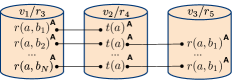
(a) All derivation trees are individually stored.

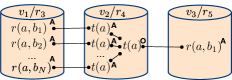
(b) All derivation trees rooted with $t(\alpha)$ are collapsed.

Figure 2. Different ways of storing $\Gamma$ in Example 1. The superscript A (O) means that the fact is labeled with $\mathsf{AND}$ ($\mathsf{OR}$). For clarity, edges to facts in $\mathcal{F}$ are not shown.

Example 0.

Consider a program with the following the three rules

($$r_{3} r(X,Y) \leftarrow q(X,Y)$$)

($$r_{4} t(X) \leftarrow r(X,Y)$$)

($$r_{5} r(X,Y) \leftarrow t(X)\wedge s(X,Y)$$)

and let $\mathcal{F}$ be a set of facts that include $q(a,b_{i})$, for ${1\leq i\leq N}$, and $s(a,b_{1})$. Figure 2a shows the lineage TG $\Gamma$ for the corresponding program and the derivation trees stored within the nodes in $\Gamma$ (for clarity, edges to facts in $\mathcal{F}$ are not shown). Node $v_{2}$ stores $N$ different trees with ${t(a)}$ as root. $N-1$ of such trees, combined with $s(a,b_{1})$ by rule $r_{5}$, lead to $N-1$ trees with $r(a,b_{1})$ as root, to be stored in $v_{3}$.

Example 1 shows that a more space-efficient technique would be to keep only the derivation tree for ${t(a)}$ in node $v_{2}$ so that only one tree with root ${r(a,b_{1})}$ is added to $v_{3}$. The challenge in doing so is to remember that $t(a)$ can be inferred in $N$ different ways.

To address this issue, we first introduce an additional label called $\mathsf{OR}$. Recall that in Section 4, all nodes in derivation trees are labeled with $\mathsf{AND}$. Intuitively, facts labeled with $\mathsf{OR}$ differ from them because they hold if only one ancestor holds. Then, we define the process of collapsing multiple derivation trees into one as follows.

Definition 0.

Let $\tau_{1},\tau_{2},\dots,\tau_{m}$ be a collection of derivation trees that have the same root fact $\alpha$. Then, $\mathsf{collapse}(\tau_{1},\tau_{2},\dots,\tau_{m})$, where $m>1$, is the derivation tree $\tau$ defined as follows:

1. $\mathsf{root}(\tau)$ is fact $\alpha$ and it is labeled with $\mathsf{OR}$; and

2. there exists an edge from $\mathsf{root}(\tau)$ to each $\mathsf{root}(\tau_{i})$.

By collapsing the derivation trees, we can reduce the number of future rule instantiations. For instance, Figure 2b shows the effect of this operation on Example 1. Here, all trees in $v_{2}$ with $t(a)$ as root are collapsed into a single entry. When rule $r_{5}$ is applied on $v_{2}$, then $t(a)$ is considered only once, which leads to the derivation of one tree instead of $N-1$ ones.

If there are no $\mathsf{OR}$-labeled nodes, then collecting the lineage of a derivation tree simply consists of collecting the leaves. Otherwise, the process has to be amended so that the branches introduced by $\mathsf{OR}$-labeled nodes are unfolded into multiple trees. We formalize the notion of unfolding derivation trees as follows.

Definition 0.

The unfolding $\mathsf{unfold}({\tau})$ of a derivation tree $\tau$ with $\mathsf{children}(\mathsf{root}(\tau))=\{\tau_{1},\dots,\tau_{m}\}$ is:

• $\{\tau\}$, if no node in $\tau$ has label $\mathsf{OR}$; or

• $\bigcup\nolimits_{\tau_{i}}\mathsf{unfold}({\tau_{i}})$, if $\mathsf{root}(\tau)$ has label $\mathsf{OR}$; or,

• $\Delta$, where, for each combination of trees ${(\delta_{1},\dots,\delta_{m})}$ from ${\mathsf{unfold}({\tau_{1}})\times\dots\times\mathsf{unfold}({\tau_{m}})}$, $\Delta$ includes a derivation tree $\varepsilon$, such that $\varepsilon$ has the same root fact as $\tau$, label $\mathsf{AND}$, and there is an edge from each $\mathsf{root}(\delta_{i})$ to $\mathsf{root}(\varepsilon)$.

In Definition 3, $\star$ regards the case where no collapsing took place; $\dagger$ regards the case where multiple derivation trees have been collapsed into one via Definition 2 so that the root of the new tree is an $\mathsf{OR}$-labelled node; finally, $\ddagger$ regards the case where $\mathsf{OR}$ appears in an ancestor of $\tau$. We illustrate Definition 3 over Example 1.

Example 0.

Suppose that all trees in node $v_{2}$ have been collapsed into a single tree $\epsilon$ with root $t(a)$, see Figure 2b, and that node $v_{3}$ stores a single derivation tree $\tau$ with the $\mathsf{AND}$-labeled fact $r(a,b_{1})$ as root. We discuss the process of unfolding $\tau$. Due to the presence of the $\mathsf{OR}$-labelled node $t(a)$ in a non-root node of $\tau$, $\mathsf{unfold}({\tau})$ will fall into case $\ddagger$ and be defined as the set of trees constructed by computing the Cartesian product of the unfoldings of the two children of $\mathsf{root}(\tau)$, i.e., $\epsilon$ and the tree with single node $s(a,b_{1})$ (the latter is not shown in Figure 2b). Since $\epsilon$ is an $\mathsf{OR}$-labeled node, $\mathsf{unfold}({\epsilon})$ is defined as the union of the unfoldings of its children, i.e., the $N$ trees with root $t(a)$ (case $\dagger$). Since none of them has an $\mathsf{OR}$-labelled node, their unfoldings are defined by the base case ($\star$), which are the trees themselves.

As a collapsed tree $\tau$ encapsulates multiple ways to derive the same fact, we say that $\tau$ is redundant w.r.t. fact $\alpha$ if $\alpha$ occurs at least twice in every derivation tree in $\mathsf{unfold}({\tau})$. This means that if we need to check whether $\tau$ is redundant, then we do not always need to fully compute $\mathsf{unfold}({\tau})$ because we can we stop as soon as we find one non-redundant derivation tree. Returning to Example 4, $r(a,b_{1})$ occurs twice in one derivation tree in $\mathsf{unfold}({\tau})$. However, $\tau$ is not redundant w.r.t. $r(a,b_{1})$ as it contains other trees in which $r(a,b_{1})$ occurs only once.

Algorithm 2 $\mathsf{PCOReason}(\mathcal{P})$, where $\mathcal{P}=(\mathcal{R},\mathcal{F},\pi)$

1:${k\mathrel{\hbox to0.0pt{\raisebox{1.29167pt}{$\cdot$}\hss}\raisebox{-1.29167pt}{$\cdot$}}=0}$;   $G^{0}$ is an empty EG for $\mathcal{R}$;

2:do

3:     ${k\mathrel{\hbox to0.0pt{\raisebox{1.29167pt}{$\cdot$}\hss}\raisebox{-1.29167pt}{$\cdot$}}=k+1}$;

4:     Compute $G^{k}$ starting from $G^{k-1}$ in an incremental fashion

5:     for each node $v$ of depth $k$ do

6:         $\mathcal{T}\mathrel{\hbox to0.0pt{\raisebox{1.29167pt}{$\cdot$}\hss}\raisebox{-1.29167pt}{$\cdot$}}=\{\mathsf{T}(\alpha,v,\mathcal{F})\neq\emptyset\mid\alpha$ is a fact$\}$   $\mathsf{tset}(v,\mathcal{F})\mathrel{\hbox to0.0pt{\raisebox{1.29167pt}{$\cdot$}\hss}\raisebox{-1.29167pt}{$\cdot$}}=\emptyset$

7:         for each ${\{\tau_{1},\dots,\tau_{n}\}\in\mathcal{T}}$ do

8:              if the average size of sets in $\mathcal{T}$ is $\geq t$ then

9:                  $Z\mathrel{\hbox to0.0pt{\raisebox{1.29167pt}{$\cdot$}\hss}\raisebox{-1.29167pt}{$\cdot$}}=\{\mathsf{collapse}(\tau_{1},\dots,\tau_{n})\}$

10:              else $Z\mathrel{\hbox to0.0pt{\raisebox{1.29167pt}{$\cdot$}\hss}\raisebox{-1.29167pt}{$\cdot$}}=\{\tau_{1},\dots,\tau_{n}\}$               

11:              for each tree $\tau\in Z$ do

12:                  if $\tau$ is not redundant w.r.t. $\alpha$ then

13:                       add $\tau$ to $\mathsf{tset}(v,\mathcal{F})$                                           

14:         if $\mathsf{tset}(v,\mathcal{F})=\emptyset$ then remove $v$ from $G$               

15:while $0pt{G^{k}}\neq 0pt{G^{k-1}}$

16:return $G^{k}(\mathcal{F})$

 Note: $t$ is a given threshold value (default value is 10).

We outline in Algorithm 2, under the name Probabilistic COllapsed Reasoning ($\mathsf{PCOReason}$), the reasoning when some derivation trees may be collapsed. The procedure proceeds similarly as in Algorithm 1. Firstly, it computes all different derivation trees that can be obtained via rule instantiations (line 6). Then, the algorithm processes one by one all the sets of trees that share the same fact $\alpha$ as root. The condition in line 8 decides whether the trees in $v$ should be collapsed using the threshold value (see discussion below). If they should be, then every set of trees is collapsed as in Definition 2. Otherwise, they are processed one-by-one (lines 11-13).

Several strategies can be implemented to decide whether to collapse the derivation trees within a node. In line 8, we use a simple threshold value and leave more complex strategies for future work. Our strategy takes into account the average number of derivation trees within a node having the same root fact. If that average is at least $t=10$ (we chose the value 10, as it sets a reduction of at least one order of magnitude), then we collapse the derivation trees in that node; otherwise, we store the trees one by one.

The following result establishes the correctness of Algorithm 2.

Theorem 5.

For each probabilistic program $\mathcal{P}$, $\mathsf{PCOReason}(\mathcal{P})$ is a lineage TG for $\mathcal{P}$.

The above result follows from the close relationship between Algorithm 1 and Algorithm 2 and the correctness of the notion of redundancy with $\mathsf{OR}$-labeled nodes.

Our technique for collapsing the lineage is similar to the technique from (Deutch et al., 2014) for computing provenance circuits. A provenance circuit is a DAG of Boolean operators and facts which can represent provenance in a compact fashion avoiding the exponential blow-up of techniques based on provenance semirings (Green et al., 2007). In (Deutch et al., 2014), the authors provided an algorithm for computing provenance via propagating circuits during the computation of the model. The technique first creates a circuit that includes every fact in the database. Then, at each round $k$, it instantiates all rules using at least one fact derived in the ${(k-1)}$-th round– that is the constrained introduced by SNE, see Section 2. If such an instantiation ${\alpha\leftarrow\alpha_{1}\wedge\dots\wedge\alpha_{N}}$ is not possible, the computation terminates. Otherwise, it takes the following steps. If $\alpha$ is derived for first time, then it adds two $\vee$-nodes to the circuit, one annotated with the fresh variable $X_{\alpha}$ and the second with the fresh variable $Y_{\alpha}$. Then, it adds a fresh $\wedge$-node $u$ and an edge from $X_{\alpha}$ to $u$. Finally, for each $\alpha_{i}$, it adds an edge from $u$ to the node annotated with $X_{\alpha_{i}}$, if $\alpha_{i}$ is an input fact, and, otherwise, to $Y_{\alpha_{i}}$.

Example 0.

Figure 3 presents the circuit computed out of the probabilistic program from Example 1. The label of each node is shown at the top of it. If a fact has been derived by a rule, then the associated variable has as a superscript the round in which it was created, i.e., variable $X^{1}_{r(a,b_{1})}$ is created during the first round.

The $\vee$ ($\wedge$) nodes in the provenance circuit fulfill the same function as the $\mathsf{OR}$ ($\mathsf{AND}$) labels. However, the way our approach collapses the lineage is significantly different. Firstly, our approach collapses only the lineage stored within a single TG node. Instead, in (Deutch et al., 2014), the collapsing considers the entire model as the technique is based on SNE and not on TGs. Secondly, our approach is adaptive as the collapsing is activated only if it is beneficial (see lines 8–9 of Algorithm 2). In contrast, in (Deutch et al., 2014), the operation is always performed, even when not needed. For instance, in Example 6 two fresh nodes are created for each $r(a,b_{i})$ fact. Instead, the collapsed tree representation in Figure 2 stores each $r(a,b_{i})$ fact once.

Figure 3. The provenance circuit from (Deutch et al., 2014) for Example 1.

6. Evaluation

Table 2. The considered benchmarks. In Smokers and VQAR, #DB and #DR depend on $N$ and on each query, respectively.

	#R	#DB	#DR	#Q
LUBM010	$127$	$1$M	$1.7$M	$14$
LUBM100	$127$	$12$M	$18$M	$14$
DBpedia	$9$k	$29$M	$33$M	$50$
Claros	$2$k	$13$M	$8$M	$50$
YAGO5	$221$	$1$M	$1$M	$50$
YAGO10	$396$	$1$M	$1$M	$76$
YAGO15	$571$	$1$M	$1$M	$50$
WN18RR5	$66$	$86$k	$87$k	$20$
WN18RR10	$116$	$86$k	$87$k	$20$
WN18RR15	$166$	$86$k	$87$k	$50$
Smokers	$5$	*	*	$110$
VQAR	$6$	*	*	$1000$

We implemented our approach in a new engine called LTGs and evaluated its performance against $\mathsf{ProbLog2}$ (Vlasselaer et al., 2016) that implements $\mathit{Tc}_{\mathcal{P}}$, $\mathsf{vProbLog}$ (Tsamoura et al., 2020), the state-of-the-art implementation of $\Delta\mathit{Tc}_{\mathcal{P}}$, and $\mathsf{Scallop}$ (Huang et al., 2021), a recent approximate probabilistic reasoning engine. To our knowledge, these are the only state-of-the-art engines for reasoning under the possible world semantics. We ran LTGs both with and without collapsing the lineage denoting the cases by “LTGs w/” and “LTGs w/o”, respectively.

To compute the probabilities of the answers given their lineage, we considered three state-of-the-art tools: PySDD (Darwiche, 2011), the d-tree compiler from (Fink et al., 2013) and c2d (Darwiche, 2004). PySDD is a well-known WMC solver that can process formulas in Disjunctive Normal Form (DNF), the form of the lineage returned by LTGs. PySDD will be our default solver, as it is adopted by all our competitors and supports DNF. The d-tree compiler is an alternative technique with competitive performance. Finally, c2d is another state-of-the-art solver that was ranked among the top three in the 2021 Model Counting Competition (https://mccompetition.org/). This solver requires formulas in Conjunctive Normal Form (CNF). To convert lineage formulas from DNF to CNF we applied the relaxed Tseitin transformation (Van den Broeck et al., 2014) that works in polynomial time in the size of the input formula.

All experiments ran on an Ubuntu 16.04 PC with an Intel i7 CPU and 94 GiB RAM.

6.1. Benchmarks

We considered benchmarks originating from the database, the probabilistic programming, and the machine learning communities.

• LUBM (Guo et al., 2011) is a popular Datalog benchmark that has been used to evaluate $\mathsf{ProbLog2}$, $\mathsf{vProbLog}$ and other engines (Nenov et al., 2015; Urbani et al., 2016; Tsamoura et al., 2021a). We considered LUBM010 and LUBM100 that include 1M and 12M facts, respectively. We used the set of same 127 rules with our competitors and the 14 available queries.

• DBpedia (Bizer et al., 2009) is one of the most well-known KGs built from Wikipedia. Claros (Rahtz et al., 2011) is an ontology of cultural heritage.

• Smokers (Domingos et al., 2008) is a popular KB in the AI community. The KB includes PDBs encoding random power-law graphs of $N$ nodes and up to $2\times N$ undirected edges. We considered $N$ between 10 and 20 as in (Tsamoura et al., 2020) and the 110 available queries. We limit the maximum reasoning depth to four and five steps as in (Tsamoura et al., 2020).

• VQAR (Huang et al., 2021) has been proposed for rule-based reasoning in the context of visual question answering. The benchmark provides over 5000 pairs of queries and probabilistic programs. Each program includes (i) uncertain facts obtained by translating into relational form neural predictions on images and (ii) rules and facts taken from the CRIC ontology (Gao et al., 2019). We considered the 1000 queries requiring the most reasoning steps. VQAR is challenging because the number of derivations explodes combinatorially.

Table 3. Total time (default is ms) to answer the queries in LUBM010 and LUBM100 with $\mathsf{ProbLog2}$ (P), $\mathsf{Scallop}$ (S), $\mathsf{vProbLog}$ (vP) and LTGs (L). Probabilities are computed via PySDD (SDD), d-tree and c2d. Shaded cells contain the best times.

$Q_{1}$ $Q_{2}$ $Q_{3}$ $Q_{4}$ $Q_{5}$ $Q_{6}$ $Q_{7}$ $Q_{8}$ $Q_{9}$ $Q_{10}$ $Q_{11}$ $Q_{12}$ $Q_{13}$ $Q_{14}$ $Q_{1}$ $Q_{2}$ $Q_{3}$ $Q_{4}$ $Q_{5}$ $Q_{6}$ $Q_{7}$ $Q_{8}$ $Q_{9}$ $Q_{10}$ $Q_{11}$ $Q_{12}$ $Q_{13}$ $Q_{14}$ P+SDD 59 NA NA NA NA NA NA NA NA NA NA 78 NA 150 NA NA NA NA NA NA NA NA NA NA NA NA NA NA S(30)+SDD 1.3s NA 729 NA 4.5s 817s 6s NA NA NA 63 165s 30s 326 15.5 NA 8.9s NA NA NA NA NA NA NA 372 NA NA 3.3s vP+SDD 587 7.2s 306 5.6s 13.6s NA 6.3s NA NA 1.3s 2s 17.3s 12.4s 3.1s 7.3s NA 2.5s NA NA NA NA NA NA NA 2s NA NA 38.7s L w/o+SDD 57 420 38 1.1s 1.3s NA 353 35.1s 348s 187 7 10.6s 541 337 647 52s 455 2.4s 4.7s NA 2s 51.8s NA 1.7s 31 12.7s 6.1s 4.9s L w/+SDD 49 383 38 175 365 NA 315 21.8s 174s 162 5 387 176 273 617 46.1s 444 1.5s 3.7s NA 1.9s 71.4s NA 1.6s 21 1.6s 2.8s 6s L w/+d-tree 49 676 40 461 595 NA 4.9s 668s 108s 1.5s 6 1s 206 273 617 42s 411 1.7s 2.7s NA 6.3s 658s NA 2.9s 21 2s 2.4s 6s L w/+c2d 49 41s 316 3.9s 62s NA 27s NA NA 2.4s 6 13s 6.2s 273 617 NA 1s 7.4s 113s NA 32s NA NA 4.2s 21 16s 16s 6s

Rule mining benchmarks. We also considered scenarios in which the rules are mined using AnyBurl (Meilicke et al., 2019), a state-of-the-art KG completion technique that outperforms both prior KG embedding techniques, e.g., ComplEx (Lacroix et al., 2018), and other rule mining techniques. Each rule that is mined by AnyBurl is assigned a confidence value based on its support in the data. To mine rules, we considered two KGs frequently used by the machine-learning community: YAGO3 (Mahdisoltani et al., 2014) (called YAGO thereafter) and WN18RR (Dettmers et al., 2018). For each KG, we created three different benchmarks by choosing for each predicate the top 5, 10, and 15 rules with the highest confidence. Both YAGO and WN18RR come with sets of training, validation, and testing KG triples. The training and validation triples are used to mine rules, while the testing triples are used at reasoning time.

Each benchmark ${B}$ forms the basis to create different scenarios. Each scenario is constructed from the databases, the rules, and the queries in ${B}$. We denote scenarios by writing the name of the benchmark followed by possible parameters, e.g., $\textsc{Smokers}4$ uses the Smokers KB and sets the max reasoning depth to four. Only Smokers and VQAR define the probability function $\pi$. For the remaining benchmarks, we implemented $\pi$ by assigning to each fact a random number within ${(0,1]}$. This is the same approach used in $\mathsf{ProbLog2}$ and $\mathsf{vProbLog}{}$ (Tsamoura et al., 2020). We created queries of 1, 2, 3, and 4 atoms for benchmarks not providing queries, using the method from (Joshi et al., 2020). The resulting queries require a variable number of reasoning steps to be answered. Table 2 reports statistics for all scenarios. #R, #DB, #DR and #Q denote the number of rules, facts, distinct fact derivations and total number of queries.

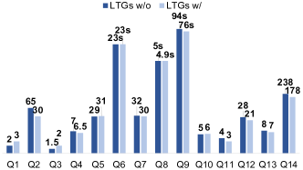
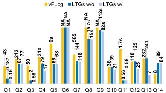
Reasoning Lineage Probability LUBM010 LUBM100

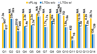
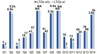
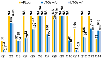
Figure 4. Runtime breakdown in ms to answer the LUBM queries.

LUBM100

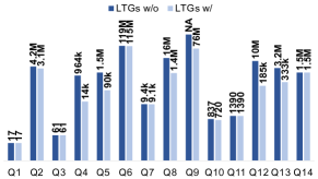
Figure 5. Number of derivations for the LUBM queries.

6.2. QA methodology

To align with the evaluation of $\mathsf{ProbLog2}$ and $\mathsf{vProbLog}$, we applied the magic sets (MS) transformation (Beeri and Ramakrishnan, 1991; Bancilhon et al., 1986; Benedikt et al., 2018). MS is a database technique that, given a query and a non-probabilistic program $\mathcal{P}$, rewrites the rules in $\mathcal{R}$ so that the bottom-up evaluation of the rewritten rules mimics the top-down evaluation of the query using $\mathcal{R}$. Tsamoura et al. (2020) have shown that MS also supports probabilistic programs.

Our experimental methodology for all scenarios other than the VQAR ones proceeds as follows. For each scenario with program ${\mathcal{P}=(\mathcal{R},\mathcal{F},\pi)}$ and query $Q$, $\mathcal{P}$ is transformed into a new program $\mathcal{P}^{Q}$ using MS. In $\mathsf{ProbLog2}$, $\mathsf{vProbLog}$, and $\mathsf{Scallop}$, query answering first computes the least parameterized model $\mathcal{M}$ of $\mathcal{P}^{Q}$ (reasoning step). Then, for each query fact $Q(\mathbf{c})$ in $\mathcal{M}$, we compute the probability of its associated formula (probability computation step). Query answering in LTGs firstly computes the lineage TG $G$ for $\mathcal{P}^{Q}$ (reasoning step), then the lineage of each $Q(\mathbf{c})$ in $G(\mathcal{F})$ (lineage collection step) and, finally, the probability of the lineage (probability computation step). With VQAR, we did not apply MS but used directly the queries proposed by $\mathsf{Scallop}$’s authors (Huang et al., 2021).

Table 4. Absolute (ms) and relative runtime overhead for collapsing the lineage during reasoning.

	LUBM010	LUBM100		LUBM010	LUBM100
Q1	0.009 (0.01%)	0.007 (0.001%)	Q8	28 (1.7%)	27 (0.6%)
Q2	1.6 (0.5%)	54 (0.1%)	Q9	115 (0.7%)	1165 (0.7%)
Q3	0.02 (0.05%)	0.01 (0.002%)	Q10	151 (0.1%)	0.2 (0.01%)
Q4	0.8 (0.4%)	0.7 (0.04%)	Q11	0.03 (0.6%)	0.04 (0.1%)
Q5	2.8 (1%)	3 (0.1%)	Q12	6.3 (1.5%)	6 (0.3%)
Q6	204 (3.4%)	2239 (2.8%)	Q13	1.6 (0.8%)	17 (0.8%)
Q7	183 (0.1%)	0.3 (0.01%)	Q14	0.9 (6.9%)	10 (6.5%)

Table 5. Average runtime (ms) and standard deviation for computing probability per query answer for LUBM010.

	vProbLog	LTGs w/
	+ PySDD	+ PySDD	+ d-tree	+ c2d
Q1	7.5 $\pm$0.1	0.001 $\pm$0.0008	0.001 $\pm$0.0007	0.002 $\pm$0.0007
Q2	7.3 $\pm$ 0.2	3.6 $\pm$1.7	13 $\pm$27	1.5s $\pm$389
Q3	7.4 $\pm$0.08	0.06/0.1	0.2 $\pm$0.08	78 $\pm$9
Q4	7.4 $\pm$ 0.07	0.5 $\pm$0.7	8.9 $\pm$49	146 $\pm$182
Q5	7 $\pm$0.08	0.1$\pm$0.1	0.4 $\pm$2	119 $\pm$80
Q6	NA	NA	NA	NA
Q7	7.1 $\pm$0.07	1.9 $\pm$1.3	70 $\pm$163	443 $\pm$164
Q8	NA	2 $\pm$1.3	84 $\pm$110	521 $\pm$147
Q9	NA	33 $\pm$39	6 $\pm$10	TO
Q10	7.5 $\pm$0.09	6 $\pm$2	358 $\pm$200	614 $\pm$163
Q11	6.9 $\pm$ 0.08	0.0009 $\pm$0.0003	0.0008 $\pm$0.0007	0.002 $\pm$0.0005
Q12	7.5 $\pm$ 0.09	2.6 $\pm$1	44 $\pm$36	980 $\pm$59
Q13	6.8 $\pm$ 0.04	0.2 $\pm$0.2	1 $\pm$1	234 $\pm$75
Q14	6.9 $\pm$0.3	0.0008 $\pm$0.0005	0.0007 $\pm$0.001	0.002 $\pm$0.0008

LTGs, $\mathsf{ProbLog2}$, and $\mathsf{vProbLog}$ are exact probabilistic reasoning engines, while $\mathsf{Scallop}$ is an approximate one that keeps only the top-$k$ explanations for each derived fact. To ensure a fair comparison, we configured $\mathsf{Scallop}$ so that the number of computed explanations is as close as possible to the ones computed by other exact engines. To this end, we set $k=30$ as the default value, the highest possible value for which $\mathsf{Scallop}$ can answer most queries (for higher values, the computation goes out of memory most of the time). Notice that even with $k=30$, $\mathsf{Scallop}$ still approximates in some cases, having an advantage. We use $\mathsf{Scallop}$($k$) to indicate $\mathsf{Scallop}$ applied for a specific $k$. We observed that when query answering terminates, it does so within a few minutes. Therefore, we set a 30 minutes timeout to let as many queries to be answered as possible without waiting for too long.

6.3. Results

For LUBM, we present a comparison between LTGs and all the other engines. For DBpedia, Claros, Smokers, YAGO, and WN18RR, the comparison does not consider $\mathsf{ProbLog2}$ and $\mathsf{Scallop}$. Regarding $\mathsf{ProbLog2}$, its performance in LUBM010 turned out to be too low to be further considered, as also observed by (Tsamoura et al., 2020). Regarding $\mathsf{Scallop}$, either it did not support some rules in the benchmarks or the data was too large to be loaded ($\mathsf{Scallop}$’s authors’ highlight scalability as a direction for future work (Huang et al., 2021)).

For VQAR, we show a comparison only between LTGs w/ and $\mathsf{Scallop}$: neither LTGs w/o nor $\mathsf{vProbLog}$ were able to compute the least parameterized model due to the combinatorial explosion of the derivations. LTGs is the only technique that can compute the full least parameterized model despite this explosion.

Notice that computing the full lineage does not necessarily mean that we can always compute its exact probability, as the problem is #P-hard (Van den Heuvel et al., 2019). To deal with such cases, approximations can be employed either upfront, by reducing the size of the lineage ($\mathsf{Scallop}$) or after the full lineage has been collected like (Gatterbauer and Suciu, 2014; Van den Heuvel et al., 2019; Olteanu et al., 2010). Approximating the probability of the lineage is an orthogonal problem. Hence, we leave the integration of such techniques with LTGs as future work, focusing on the queries for which the answers’ probabilities can be computed exactly using PySDD. In VQAR, these are 417/1000 queries. For the remaining ones, either PySDD fails or the lineage is too large ($>1M$ disjuncts) that fully computing it, although possible in some cases, goes beyond the timeout.

Overview of the experimental results. Table 3 reports the total runtime to answer the queries in LUBM010 (left-hand side) and LUBM100 (right-hand side) using all engines. In LTGs, the total runtime is the sum of the reasoning, lineage collection, and probability computation times. Figure 4 shows a breakdown of the above steps for $\mathsf{vProbLog}$ and LTGs. Lineage collection is not relevant to $\mathsf{vProbLog}$, since $\Delta\mathit{Tc}_{\mathcal{P}}$ does not require this step. Figure 5 shows the number of derivations produced when answering the LUBM queries using LTGs. The number of derivations is a rough estimator of the difficulty of each query and is independent of the implementation. “NA” in Table 3 and Figures 4 and 5 denotes either timeout or out of memory (a detailed breakdown is shown later). Table 4 shows the overhead (both absolute in ms and relative to the total reasoning time) to collapse the lineage on LUBM, while Table 5 reports the average runtime in ms to compute the probabilities of the query answers using different techniques.

Figure 6 reports the reasoning, probability computation, and the total query answering time for the DBpedia, Claros, Smokers, YAGO, and WN18RR scenarios. The figures under “Derivations” show the number of derivations for LTGs. We used boxplots since the number of queries per scenario is large. The boxplots aggregate the times of all queries whose evaluation is completed within 30 minutes. For Smokers, $k$ indicates the maximum reasoning depth which can be either four or five. In contrast, the different $k$’s in the YAGO and WN18RR scenarios denote the number of highest confidence rules kept per predicate. Table 6 reports the number of queries whose evaluation was not completed within the timeout (“TO” column) or which ran out of memory (“OOM” column) (the # queries per scenario is in Table 2). For the queries that were successfully answered, we recorded the peak RAM used by the engine. Table 6 reports the min and max values obtained in each scenario (denoted by its initial, e.g., “L” denotes LUBM) to show the memory requirements in the best and worst case.

Figures 7a, 7b, and 7c report results collected from the 417 VQAR queries for which LTGs w/ can compute exact answers. To show the impact of the approximation on runtime, Figure 7a reports a comparison of the total runtime needed by $\mathsf{Scallop}$(1) (S(1)), $\mathsf{Scallop}$(20) (S(20)), and LTGs w/ (Total LTGs). For LTGs w/, the figure also reports a breakdown of the runtime needed for reasoning (Reas.), lineage collection (Lin.), and probability computation (Prob.). All times are in ms. Since our engine allows exact query answering, we also evaluate the impact of approximations on the answers’ probabilities, i.e., we assess how close the approximate probabilities to the actual ones are. To this end, Figure 7b reports the relative probability errors of the answers computed by $\mathsf{Scallop}$(1) and $\mathsf{Scallop}$(20). The relative probability error of an answer $\alpha$ is computed by $(\epsilon_{\alpha}-\hat{\epsilon}_{\alpha})/\epsilon_{\alpha}$, where $\epsilon_{\alpha}$ denotes the exact probability (as computed by LTGs) and $\hat{\epsilon}_{\alpha}$ the approximation. In this experiment, the 417 queries produced 5949 answers. Figure 7b groups the answers based on their relative errors and reports the total number of answers within each group, i.e., regarding S(1), there are 168 answers for which the error falls in $[0,10\%)$. Finally, to provide some anecdotal evidence, we chose the 5/417 queries that $\mathsf{Scallop}$ takes the most time to answer for different $k$’s. Table 7c presents the total runtime of those queries with $\mathsf{Scallop}$ and LTGs w/, and the highest probabilities of their answers.

Table 6. Min and max peak RAM usage (GB) to answer the benchmark queries and # of OOM and TO queries.

	vProbLog		LTGs w/o		LTGs w/
	Min/Max	OOM/TO	Min/Max	OOM/TO	Min/Max	OOM/TO
L10	11/11	1/2	1.7/19	1/0	1.9/11	1/0
L100	13/14	2/12	1.8/5.7	2/0	1.9/4.8	2/0
D	30/38	3/0	2/4.9	3/0	1.9/2.5	3/0
C	19/20	3/0	2.5/6.1	3/0	2.4/5.2	3/0
Y5	11/11	12/8	1.8/1.8	12/0	1.8/1.8	11/0
Y10	11/11	30/19	1.8/1.8	25/0	1.8/1.8	25/0
Y15	11/11	12/18	2.4/2.4	12/8	1.7/1.7	12/8
W5	11/11	0/0	1.8/1.8	0/0	1.8/1.8	0/0
W10	11/11	0/0	1.8/1.9	0/0	1.8/1.8	0/0
W15	11/11	0/0	1.9/1.9	0/0	1.8/1.8	0/0
S4	11/11	0/0	1.7/1.7	0/0	1.7/17	0/0
S5	11/11	0/0	1.8/17	0/0	1.7/19	0/0
V		1000/0		1000/0	1.4/24	560/23

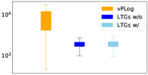
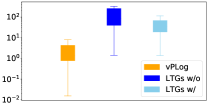
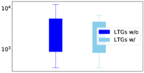
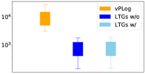
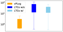
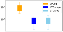
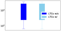
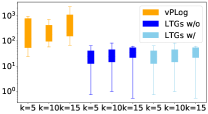
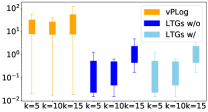
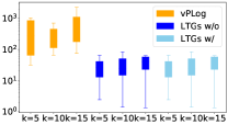
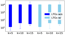
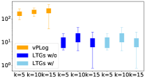
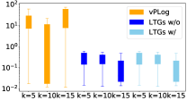
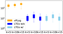
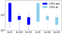
Reasoning (ms) Probability (ms) Total (ms) Derivations DBpedia Claros YAGO WN18RR Smokers

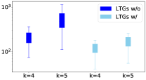
Figure 6. Time in ms to answer queries and total number of derivations for different scenarios with $\mathsf{vProbLog}$ and LTGs.

6.4. Key conclusions

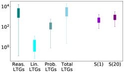
(a)

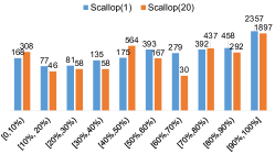
(b)

	Query ID	2343894_40	2327997_45	2322829_40	2416754_49	2346575_46
Runtime	$\mathsf{S}(1)$	1.5s	800ms	721ms	793ms	1.1s
	$\mathsf{S}(20)$	1311s	148s	88s	45s	40s
	$\mathsf{S}(30)$	TO	1415s	89s	42s	41s
	LTGs w/	353s	7.3s	6.1s	20s	17.6s
Probability	$\mathsf{S}(1)$	0.03	0.003	0.04	0.006	0.68
	$\mathsf{S}(20)$	0.12	0.02	0.05	0.007	0.97
	$\mathsf{S}(30)$	TO	0.02	0.05	0.007	0.97
	LTGs w/	0.13	0.02	0.11	0.015	0.97

(c)

Figure 7. Results related to the 417 VQAR queries that LTGs can answer exactly. (a) Runtime breakdown for LTGs w/ and total runtime in ms for $\mathsf{Scallop}$; (b) relative probability errors obtained when approximating; (c) anecdotal evidence with five queries.

C1: LTGs outperforms prior art in terms of runtime. Table 3 and Figure 6 indicate that query answering with LTGs is faster than with the other engines. For instance, the maximum total runtime drops from 195s in DBpedia and 26s in Claros with $\mathsf{vProbLog}$, to 129s and 11s, respectively, with LTGs. The average total runtime drops from 14s (DBpedia) and 8s (Claros) with $\mathsf{vProbLog}$, to 6.6s and 1.4s respectively, with LTGs. The improvements are even larger for YAGO and WN18RR: the mean runtime drops from 0.7s to 0.1s in YAGO15 and from 0.2s to 0.01s in WN18RR15.

More importantly, LTGs can mean the difference between answering and not answering the query at all. For instance, LTGs can successfully answer 13/14 queries in LUBM010 (most of them in the order of seconds) and 12/14 queries in LUBM100. Regarding $Q_{6}$ in LUBM010, LTGs completed reasoning and lineage collection successfully, but PySDD ran out of memory. Regarding $Q_{6}$ and $Q_{9}$ in LUBM100 using LTGs, it is lineage collection that ran out of memory: reasoning finished successfully. In comparison to $\mathsf{vProbLog}$, which is the second-best exact engine, LTGs is faster in all queries except for the ones in which both systems time out, with the improvements brought by LTGs being more than one order of magnitude, see $Q_{1}$ and $Q_{5}$. Table 3 also shows that LTGs is often faster than $\mathsf{Scallop}$(30), outperforming it in all cases except $Q_{6}$ in LUBM010, where $\mathsf{Scallop}$ returns approximate answers in 817s, and $Q_{14}$ in LUBM100. Regarding $Q_{6}$, the probability computation done by LTGs is intrinsically expensive and hence $\mathsf{Scallop}$, which does approximations, runs faster. Regarding $Q_{14}$, the query requires almost no reasoning and $\mathsf{vProbLog}$ had a lower overhead.

C2: Collapsing the lineage can significantly improve the performance. Consider, for instance, query $Q_{12}$ in LUBM010. It takes 10.6s to answer $Q_{12}$ with LTGs w/o and only 387ms with LTGs w/. This is because reasoning for $Q_{12}$ in LUBM010 takes 10s with LTGs w/o and only 341ms with LTGs w/, see Figure 4. Significant performance improvements are observed in other queries as well, e.g., $Q_{4}$ in LUBM010 and $Q_{2}$ in LUBM010. Overall, LTGs w/ is at least 25% faster than LTGs w/o in most of the cases. The biggest difference is observed in the VQAR queries, where lineage collapsing allows us to compute the full least parameterized model for all queries. The cause behind the reasoning time improvements is the drastic decrease in the number of derivations. For instance, $Q_{12}$ in LUBM010 involves 10M derivations with LTGs w/o, see Figure 5. Instead, the same query involves 185k derivations with LTGs w/. The number of derivations significantly decreases also in DBpedia and Smokers, while it remains roughly the same in the other cases, see Figure 6.

Often, the overhead introduced by the operation of collapsing the lineage is negligible (i.e., less than 1%, see Table 4). However, there are a few cases where it is not, like with $Q_{12}$ and $Q_{14}$. Regarding $Q_{12}$, even though the overhead is non-negligible, it brings an improvement in terms of runtime which outweighs the cost of collapsing. With $Q_{14}$, however, this is not the case because the query does not trigger enough reasoning to justify the operation of collapsing, rendering collapsing no longer beneficial.

C3: The runtime overhead to collect the lineage is small. In most scenarios, the overhead of computing the lineage is relatively small in comparison to the time needed for reasoning. For instance, in DBpedia and Claros, the maximum to collect the lineage is 1581 ms and 1533 ms, respectively. Since LTGs can reason more efficiently, this overhead is a fair price to pay to obtain a much lower total runtime. In LUBM, we observed two cases where the cost of lineage collection is prohibitively high: $Q_{6}$ and $Q_{9}$ in LUBM100. This is because the associated number of answers is so large that the cost of lineage collection outweighs the reduction in reasoning runtime.

C4: LTGs outperforms prior art in terms of memory. As we can see in Table 6, LTGs is up to four times more memory efficient than $\mathsf{vProbLog}$ in the LUBM scenarios; the improvements exceed the six times in the YAGO and WN18RR scenarios. This is because LTGs does not fully materialize the trees but stores instead pointers to the parent trees (structure sharing). The operation of collapsing the derivation trees further reduces the memory consumption. Looking again at Table 6, we notice that in the best case the max RAM usage is almost reduced by half (DBpedia, 4953MB vs. 2550MB). The only scenario where LTGs requires more RAM is with Smokers5 (S5), which is a case where the column-based data structures used by $\mathsf{vProbLog}$ take less space. Regarding LUBM010 and LTGs w/o, the higher maximum RAM consumption (19GM in LTGs w/o vs 11GB in $\mathsf{vProbLog}$) is due to $Q_{9}$, a query that $\mathsf{vProbLog}$ cannot answer. Although LTGs is overall more memory-efficient, there are still queries for which the RAM is not enough. The reason lies in the worst-case intractability of the problem at hand. One such example is $Q_{6}$ from LUBM010 where the reasoning and lineage collection step are computed successfully, but probability computation done by PySDD runs out of memory. A major contribution of our work is that it significantly reduces the number of such cases, see VQAR. Furthermore, the fact that in the most challenging cases LTGs reasons using 24GB of RAM hints that LTGs does not require expensive hardware for supporting complex scenarios.

C5: LTGs can be used in combination with different probability computation techniques. Table 3 shows that even when using different probability computation tools than PySDD, LTGs can have state-of-the-art performance: when combined with c2d, LTGs w/ outperforms $\mathsf{vProbLog}$ in 5/14 queries in LUBM010 and 9/14 queries in LUBM100; when using d-tree, LTGs w/ is almost always faster than $\mathsf{vProbLog}$. Table 5 shows that PySDD tends to be the most efficient library in terms of runtime, while c2d is the one with the slowest runtime per answer. This is because the translation from DNF into CNF via the Tseitin transformation creates inter-dependencies among different disjunctions of the lineage formulas that make the decomposition of the formula required by c2d harder. It is also interesting to point out that PySDD performs much better when it is coupled with LTGs than with $\mathsf{vProbLog}$. The reason is that PySDD translates the lineage into an internal form called vtree (Pipatsrisawat and Darwiche, 2008). The cost of that translation depends on the structures of the formulas, i.e., two formulas (one returned by LTGs and one returned by $\mathsf{vProbLog}$) may be logically equivalent, but the cost of translating them into vtrees may be different. This explains the discrepancy of runtimes, which was also observed in (Tsamoura et al., 2020).

C6: LTGs is competitive to approximate techniques. Unsurprisingly, approximating reasoning by keeping only the top $k$ proofs returns lower runtimes (Figure 7a). However, by doing so, the returned probabilities may be far from the actual ones. The difference can be substantial if we do aggressive approximations, like with $\mathsf{Scallop}$(1). For instance, we can see from Figure 7b that the relative error of 2357 answers (out of 5949) is greater than $90\%$. Figure 7c gives a couple of illustrative examples: the answers of queries 2322829_40 and 2416754_49 have probabilities that are at least two times lower than the actual ones. To reduce the approximation error, one would need to increase $k$, e.g., by running $\mathsf{Scallop}$(20) and $\mathsf{Scallop}$(30). However, by doing so, the runtime of $\mathsf{Scallop}$ increases to the point where it is no longer beneficial to approximate.

7. Related work

Several approaches perform reasoning under uncertainty including ICL (Poole, 2008), PRISM (Sato, 1995), MLNs (Richardson and Domingos, 2006), and PSL (Bach et al., 2017). ICL and PRISM support only rules where the same predicate cannot occur both in their premise and in their conclusion. MLNs and PSL are not based on logic programming but first-order logic. Hence, they do not support non-ground recursive rules, as first-order logic cannot specify the closure of a transitive relation (Grädel, 1992). Stochastic Logic Programs (Cussens, 2000), TensorLog (Cohen et al., 2020), and Probabilistic Datalog (Fuhr, 2000, 1995) do not support the possible world semantics. Bárány et al. (2017) proposed another probabilistic version of Datalog, called PPDL (Bárány et al., 2017). Different from our work, the semantics of PPDL is defined using Markov chains. We are not aware of any PPDL engine.

Several approaches aim to reduce the cost of computing the full lineage by computing a subset of it. The first ProbLog engine (De Raedt et al., 2007) implemented iterative deepening; ProbLog2 implements $k$-best (Gutmann et al., 2008) and $k$-optimal (Renkens et al., 2012) approximations; $\mathsf{Scallop}$ keeps the $k$ most likely explanations per fact achieving state-of-the-art performance (Huang et al., 2021). The main difference between these approaches and LTGs is that the latter performs exact reasoning. Our evaluation shows that even though LTGs must often do more work than approximate methods, there are cases where LTGs is still significantly more efficient.

A multitude of approximations techniques tackle the DNF probability computation problem (Dalvi and Suciu, 2007b; Olteanu et al., 2010; Ré and Suciu, 2008). Van den Heuvel et al. in (Van den Heuvel et al., 2019) have recently proposed an anytime approximation technique that builds upon “dissociation”-based bounds (Gatterbauer and Suciu, 2014). Integrating such techniques into LTGs is an interesting direction as it can extend applicability when the lineage is too large to be further processed.

Research of query answering over PDBs (Suciu et al., 2011) has provided us with a wealth of results, especially on tractability of complex queries, e.g., (Dalvi and Suciu, 2012, 2007a), and approximations, e.g., (Gribkoff and Suciu, 2016). Recent work includes finding explanations for queries, e.g., (Gribkoff et al., 2014), and querying subject to constraints (Friedman and den Broeck, 2019). Systems like MystiQ (Dalvi et al., 2009) and MayBMS (Antova et al., 2008) propose extensions to DBMSs like PostgreSQL for supporting the semantics of PDBs, while PrDB (Sen et al., 2009) introduces techniques extending databases with graphical models. In (Dylla et al., 2013) and (Dylla et al., 2013), Dylla et al. study the problem of answering queries over temporal PDBs and introduce techniques for top-k query answering over PDBs, respectively. In contrast to our work, the above line of research focuses on supporting SQL queries and not rule-based reasoning beyond view reformulation.

LTGs relates to high-performance Datalog engines including VLog (Urbani et al., 2016), RDFox (Nenov et al., 2015) and Vadalog (Bellomarini et al., 2018). It has been shown that (non-probabilistic) TG-based reasoning outperforms the above engines in terms of runtime and memory consumption (Tsamoura et al., 2021a). Furthermore, TG-based reasoning provides the means to naturally maintain the derivation provenance without extra overhead due to the induced TG. None of the aforementioned engines can be easily extended to that fashion, as they all implement the chase (Benedikt et al., 2017), which “disconnects” the facts from the rules that derived them.

$\mathsf{ProbLog2}$, $\mathsf{vProbLog}$, and $\mathsf{Scallop}$ closely relate to provenance semirings. Green et al. have defined provenance for Datalog using semirings that supports the possible world semantics (Green et al., 2007). The difference between (Green et al., 2007) and the aforementioned engines is that the latter improve the runtimes exploiting ideas from bottom-up Datalog evaluation. The authors in (Ramusat et al., 2021) provide an SNE, bottom-up method for approximating the provenance for a specific class of semirings for finding best-weight derivations. With the same spirit, (Deutch et al., 2018) proposes approximate provenance computation techniques, while (Dannert et al., 2021) develops semiring provenance for very general logical languages involving negation and fixed-point operations.

8. Conclusion

We presented a new scalable technique for probabilistic rule-based reasoning over PDBs which computes a compact probabilistic model, leveraging the topology of the TG and structure sharing. Our experiments show that our engine outperforms prior art both in terms of runtime and memory consumption, often significantly, and sometimes it can make the difference between answering a query in a few seconds and not answering it at all. Future research includes extending LTGs for reasoning over KG embedding models (e.g., (Friedman and den Broeck, 2020)). A promising direction is LTGs’ integration with approximate techniques that compute only part of the lineage (Poole, 1992; De Raedt et al., 2007; Gutmann et al., 2008; Renkens et al., 2012; Nitti et al., 2014; Gutmann et al., 2011), or with techniques that guide the computation of the proofs via machine learning i.e., reinforcement learning (Kaliszyk et al., 2018).

Appendix A Computing execution graphs incrementally

We elaborate on the step of incremental EG computation (line 4 of Algorithm 1 and line 4 of Algorithm 2). EGs can be computed incrementally, as it was shown by Tsamoura et al. (2021a). Suppose that we have already built an EG of depth ${k-1}$ and we want to add new nodes of depth $k$ so that we do not miss any rule execution. As the edges dictate the nodes over which we are instantiating the premises of the rules, we need to make sure that the extended EG exhaustively adds all possible edges. We refer to each combination of nodes of depth ${<k}$ whose facts may instantiate the premise of a rule $r$ when reasoning over an EG, as $k$-compatible nodes for $r$:

Definition 0.

[From (Tsamoura et al., 2021a)] A combination of $n$ nodes ${(u_{1},\dots,u_{n})}$ from $G$ is $k$-compatible with $r$, where ${k\geq 2}$ is an integer, if:

• the predicate in the head of $u_{i}$ is $p_{i}$;

• the depth of each $u_{i}$ is less than $k$; and

• at least one node in ${(u_{1},\dots,u_{n})}$ is of depth ${k-1}$.

The above ideas are summarized in an iterative procedure, which builds at each step $k$ an EG $G^{k}$ of depth $k$:

• (Base step) if ${k=1}$, then for each base rule $r$ add to $G^{k}$ a node $v$ associated with $r$.

• (Inductive step) otherwise, for each non-base rule $r$ and each combination of nodes ${(u_{1},\dots,u_{n})}$ from $G^{k-1}$ that is $k$-compatible with $r$, add to $G^{k}$: (i) a fresh node $v$ associated with $r$ and (ii) an edge ${u_{i}\rightarrow_{i}v}$, for each ${1\leq i\leq n}$.

Appendix B Proofs for Section 4

Algorithm 3 $\mathsf{Step}(\mathcal{I})$, where $\mathcal{P}=(\mathcal{R},\mathcal{F},\pi)$, $\mathcal{I}=\{(\alpha_{i},\lambda_{i})\}$, and $\lambda_{i}$ is a Boolean formula over elements in $\mathcal{F}$

1:$\mathcal{I}^{\prime}\mathrel{\hbox to0.0pt{\raisebox{1.29167pt}{$\cdot$}\hss}\raisebox{-1.29167pt}{$\cdot$}}=\emptyset$  $\Delta\mathrel{\hbox to0.0pt{\raisebox{1.29167pt}{$\cdot$}\hss}\raisebox{-1.29167pt}{$\cdot$}}=\emptyset$

2:for each rule $r$ in $\mathcal{P}$ and each instantiation $\alpha\leftarrow\alpha_{1}\wedge\dots\wedge\alpha_{n}$ of $r$, s.t. each ${(\alpha_{i},\lambda_{i})}$ is in $\mathcal{I}$ for some $\lambda_{i}$ do

3:     add ${(\alpha,\bigwedge_{i}^{n}\lambda_{i})}$ to $\Delta$

4:for each $\alpha$, s.t. a pair of the form ${(\alpha,\cdot)}$ is in $\Delta\cup\mathcal{I}$  do

5:     add ${(\alpha,\bigvee_{(\alpha,\varphi)}\varphi)\in\Delta}$ to $\mathcal{I}^{\prime}$

6:return $\mathcal{I}^{\prime}$

As stated in Section 4.2, Lemma 5 concerns the simplified versions of Algorithm 1 and $\mathit{Tc}_{\mathcal{P}}$ in which no termination condition is employed. In the case of Algorithm 1 that simplification means that the check in line 9 is avoided, so that each tree $\tau$ is added to $\mathsf{tset}(v,\mathcal{F})$. We recapitulate in Algorithm 3 the steps taking place during each iteration of simplified $\mathit{Tc}_{\mathcal{P}}$, when an instance $\mathcal{I}$ is provided in its input. Throughout, we fix a probabilistic logic program $\mathcal{P}=(\mathcal{R},\mathcal{F},\pi)$ and denote by $G^{i}$, the EG computed at the end of the $i$-th iteration of Algorithm 1 and by $G^{i}(\mathcal{F})$ the derivation trees that are stored within the nodes of $G^{i}$. We also denote by $\mathcal{I}^{i}$ the instance computed at the end of the $i$-th iteration of $\mathit{Tc}_{\mathcal{P}}$, where $\mathcal{I}^{0}=\{(f,f)\mid p::f\in\mathcal{F}\}$. The proof of Lemma 5 relies on Claim 1, which again concerns the simplified Algorithm 1.

Claim 1.

Let $\tau_{1},\dots,\tau_{n}$ be derivation trees in $G^{i}(\mathcal{F})$, for $i\geq 0$, so that each $\tau_{j}$ has root $\alpha_{j}$ and is stored in a node of depth $<i$. Let also $r$ be a rule and ${\alpha\leftarrow\alpha_{1}\wedge\dots\wedge\alpha_{n}}$ be an instantiation of it. Then, the following IH holds for each $i\geq 0$:

• $\rho$. There is a tree $\tau$ in $G^{i}(\mathcal{F})$ so that $\tau$ has root $\alpha$ and there is an edge from the root of $\tau_{j}$ to the root of $\tau$.

Proof.

For $i=0$, the IH $\rho$ trivially holds as $G^{0}$ is the empty graph by definition. For $i+1$ and assuming that $\rho$ holds for ${i\geq 0}$, we have the following. Let ${(u_{1},\dots,u_{n})}$ be the tuple of nodes in $G^{i}$, such that $\tau_{j}\in\mathsf{tset}(u_{j},\mathcal{F})$, for ${1\leq j\leq n}$. If each $u_{j}$ is of depth $<i$, then $\rho$ trivially holds. Hence, we consider the case in which at least one $u_{j}$ is of depth $i$.

As the root of each $\tau_{j}$ is $\alpha_{j}$ and due to the instantiation ${\alpha\leftarrow\alpha_{1}\wedge\dots\wedge\alpha_{n}}$, it follows from Definition 1 that ${(u_{1},\dots,u_{n})}$ is $i$-compatible with $r$. As ${(u_{1},\dots,u_{n})}$ is $i$-compatible with $r$, it follows from the step in line 4 of Algorithm 1 that $G^{i+1}$ includes a node $v$, so that the edge ${u_{j}\rightarrow_{j}v}$ is in $G^{i+1}$, for ${1\leq j\leq n}$. Furthermore, due to ${\alpha\leftarrow\alpha_{1}\wedge\dots\wedge\alpha_{n}}$, due to Definition 3 and since $\tau_{j}\in\mathsf{tset}(u_{j},\mathcal{F})$, for ${1\leq j\leq n}$, ${\mathsf{T}(\alpha,v,\mathcal{F})}$ includes a tree $\tau$ with root atom $\alpha$ and edges from the root of each $\tau_{j}$ to the root of $\tau$, where ${1\leq j\leq n}$. Tree $\tau$ will be stored in $\mathsf{tset}(v,\mathcal{F})$. As $\tau\in\mathsf{tset}(v,\mathcal{F})$, it follows that $\rho$ holds for $i+1$ concluding the proof of Claim 1. ∎

See 5

Proof.

For $i=0$, the IH holds in both directions as ${\mathcal{I}^{0}=\{(f,f)\mid p::f\in\mathcal{F}\}}$ and ${G^{0}(\mathcal{F})=\mathcal{F}}$ by definition and the lineage of a fact in $\mathcal{F}$ is the fact itself.

($\Rightarrow$) For $i+1$ and assuming that $\omega$ holds for $i$, the proof proceeds as follows. Suppose that a rule $r$ is instantiated under ${\alpha\leftarrow\alpha_{1}\wedge\dots\wedge\alpha_{n}}$ at step ${i+1}$ of $\mathit{Tc}_{\mathcal{P}}$ and let ${(\alpha_{j},\lambda^{i}_{\alpha_{j}})\in\mathcal{I}^{i}}$, for ${1\leq j\leq n}$. As the IH holds for $i$, we know that for each $\alpha_{j}$, there is a set of trees $\mathcal{T}_{j}$ in $G^{i}(\mathcal{F})$ all having the same root $\alpha_{j}$, so that $\bigvee\nolimits_{\tau\in\mathcal{T}_{j}}\phi(\tau)\equiv\lambda^{i}_{\alpha_{j}}$ holds. Furthermore, due to the IH, each tree in $\mathcal{T}_{j}$ is stored in a node of depth $\leq i$, for ${1\leq j\leq n}$. Due to the above, the formula computed out of the above rule instantiation in the step in line 3 of Algorithm 3 is given by

(3) $$\bigwedge_{j=1}^{n}\lambda^{i}_{\alpha_{j}}\equiv\bigwedge_{j=1}^{n}\bigvee\nolimits_{\tau\in\mathcal{T}_{j}}\phi(\tau)\equiv\bigvee_{(\tau_{1},\dots,\tau_{n})\in\mathcal{T}_{1}\times\dots\times\mathcal{T}_{n}}\phi(\tau_{1})\wedge\dots\wedge\phi(\tau_{n})$$

From Claim 1, we know that for each tuple ${(\tau_{1},\dots,\tau_{n})\in\mathcal{T}_{1}\dots\times\dots\mathcal{T}_{n}}$, there is a tree $\tau$ in $G^{i+1}(\mathcal{F})$ so that $\tau$ has root fact $\alpha$ and there is an edge from the root of $\tau_{j}$ to the root of $\tau$. From the above and the definition of $\phi$, ${\phi(\tau)=\phi(\tau_{1})\wedge\dots\phi(\tau_{n})}$ holds. Consequently, the lineage of $\alpha$ in $G^{i+1}(\mathcal{F})$ is given by

(4) $$\bigvee_{(\tau_{1},\dots,\tau_{n})\in\mathcal{T}_{1}\times\dots\times\mathcal{T}_{n}}\phi(\tau_{1})\wedge\dots\wedge\phi(\tau_{n})$$

Due to the above, $\omega$ holds for $i+1$: firstly, the formula $\lambda^{i+1}_{\alpha}$ associated with atom $\alpha$ at the end of the $(i+1)$-th iteration of the steps shown in Algorithm 3 is given by

(5) $$\lambda^{i+1}_{\alpha}=\lambda^{i}_{\alpha}\vee\bigvee\limits_{\alpha\leftarrow\alpha_{1}\wedge\dots\wedge\alpha_{n},s.t.(\alpha_{j},\lambda_{\alpha_{j}}^{i})\in\mathcal{I}^{i}}\bigwedge_{j=1}^{n}\lambda^{i}_{\alpha_{j}}$$

secondly, due to $\omega$, for all trees ${\tau_{1},\dots,\tau_{m}}$ in $G^{i}(\mathcal{F})$ with root atom $\alpha$, we have

(6) $$\bigvee\nolimits_{j=1}^{m}\phi(\tau_{j})\equiv\lambda^{i}_{\alpha}$$

and finally, the lineage of $\alpha$ in $G^{i+1}(\mathcal{F})$ is the disjunction the formula $\phi(\tau)$ of each $\tau$ in $G^{i+1}(\mathcal{F})$ with root fact $\alpha$.

($\Leftarrow$) The proof is analogous to the other direction and relies on Claim 1 and (3). ∎

See 6

Proof.

If $\tau^{\prime}$ is a subtree of $\tau$, then $\phi(\tau^{\prime})$ is a subconjunct of $\phi(\tau)$. As such, ${\phi(\tau)\vee\phi(\tau^{\prime})\equiv\phi(\tau^{\prime})}$ holds. ∎

See 7

Proof.

When a (probabilistic) logic program admits a finite Herbrand base, then there is a finite number of different rule instantiations. Due to the above, if we organize the rule instantiations in a graph $\Gamma$ so that $\Gamma$ includes an edge from atoms ${\alpha_{1},\dots,\alpha_{n}}$ to atom $\alpha$, for each rule instantiation ${\alpha\leftarrow\alpha_{1},\dots,\alpha_{n}}$, there will be a depth ${k>0}$ so that either there is no rule instantiation in which the atoms in the premise of a rule are of depth $<k$, or there are such instantiations, but there is a repetition in the atom derivations, in the sense, that an atom $\alpha$ of derivation depth $k$ includes $\alpha$ in its set of ancestor nodes. The above indicates that Algorithm 1 does terminate with programs admitting a finite Herbrand base. Notice that (probabilistic) Datalog programs always admit a finite Herbrand base, therefore Algorithm 1 always terminates. ∎

See 9

Proof.

Recall that according to Definition 8, an EG $G$ for a probabilistic program $\mathcal{P}$ s a lineage TG for $\mathcal{P}$, if for each atom ${\alpha\in\mathsf{HB}(\mathcal{P})\setminus\mathcal{F}}$, the lineage of $\alpha$ in $G(\mathcal{F})$ is logically equivalent to the lineage of $\alpha$ in $\mathcal{P}$. Lemma 5 guarantees an equivalence between the formulas computed out of the derivation trees and the disjuncts of the $\lambda$ formulas in the least parameterized model of $\mathcal{P}$ at each step of $\mathit{Tc}_{\mathcal{P}}$ assuming that both techniques employ no termination checks. Furthermore, Lemma 7 suggests termination of Algorithm 1 and consequently, due to Lemma 5, equivalence with least parameterized model of $\mathcal{P}$. ∎

See 10

Proof.

This follows straightforwardly from the fact that the lineage of an atom $\alpha$ in $G^{k}(\mathcal{F})$ is a disjunct of its full lineage in $G(\mathcal{F})$. ∎

Appendix C Proofs for Section 5

See 5

Proof.

The proof of Theorem 5 follows from Lemma 1, 2 and 3 which we show below. Throughout, we fix a probabilistic logic program $\mathcal{P}=(\mathcal{R},\mathcal{F},\pi)$ and denote by $G^{i}_{1}$ and $G^{i}_{2}$, the EGs computed at the end of the $i$-th iteration of Algorithm 1 and Algorithm 2.

Lemma 0.

For each $i\geq 0$, the following IH holds:

• $\xi_{1}$. for each derivation tree $\tau$ with root fact $\alpha$ that is stored in a node of depth $i$ in $G_{1}^{i}$, there exists a derivation tree $\varepsilon$ that is stored in a node of depth $i$ in $G_{2}^{i}$, such that ${\tau\in\mathsf{unfold}({\varepsilon})}$.

Proof.

For $i=0$, $\xi_{1}$ trivially holds, as both $G_{1}^{0}$ and $G_{2}^{0}$ are empty. For $i+1$ and assuming that $\xi_{1}$ holds for $i\geq 0$, the proof proceeds as follows. Let $\tau$ be a derivation tree that has been added to a node $v$ by the end of the $i+1$-th iteration of Algorithm 1. Let us assume $v$ is associated with rule $r$ and that the root of $\tau$ is a fact $\alpha$. According to the definition of redundancy from Section 5 and the steps in lines 9 and 10 of Algorithm 1, it follows that $\tau$ is not redundant w.r.t. $\alpha$. Furthermore, from Definition 3, it follows that there is an instantiation $\alpha\leftarrow\alpha_{1}\land\ldots\land\alpha_{n}$ of $r$ so that for each ${1\leq j\leq n}$, (i) there is a node $u_{j}$ of depth $\leq i$, (ii) a tree $\tau_{j}$ is stored in $\mathsf{tset}(u_{j},\mathcal{F})$ and (iii) the edge $u_{j}\rightarrow v$ is in $G_{1}^{i+1}$. Due to the step in line 4 of Algorithm 1, at least one node from $u_{1},\dots,u_{n}$ is of depth $i$. Since $\xi_{1}$ holds for $\leq i$, we have that for each ${\tau_{j}}$, there exists a derivation tree $\varepsilon_{j}$ stored in a node $u^{\prime}_{j}$ in $G_{2}^{i}$ having the same depth with $u_{j}$, so that $\tau_{j}\in\mathsf{unfold}({\varepsilon_{j}})$. Due to the step in line 4 of Algorithm 2, since at least one node in $u_{1},\dots,u_{n}$ is of depth $i$ and since the combination of nodes ${(u_{1},\dots,u_{n})}$ from $G_{1}^{i}$ is ($i+1$)-compatible with $r$ (see Definition 1), then the combination of nodes ${(u^{\prime}_{1},\dots,u^{\prime}_{n})}$ from $G_{2}^{i}$ is ($i+1$)-compatible with $r$. Hence, ${(u^{\prime}_{1},\dots,u^{\prime}_{n})}$ will be considered in line 4 at the beginning of the ($i+1$)-th iteration of Algorithm 2. Consequently, $G_{2}^{i+1}$ will include a node $v^{\prime}$ associated with rule $r$ and an edge from $u^{\prime}_{j}\rightarrow v^{\prime}$, for ${1\leq j\leq n}$. Furthermore, since for each ${1\leq j\leq n}$, $\varepsilon_{j}$ is stored in $u^{\prime}_{j}$, so that $\tau_{j}\in\mathsf{unfold}({\varepsilon_{j}})$, since the root of $\varepsilon_{j}$ is $\alpha_{i}$, since $\alpha\leftarrow\alpha_{1}\land\ldots\land\alpha_{n}$ is an instantiation of $r$ and due to Definition 3, it follows that for each ${1\leq j\leq n}$, $\mathsf{T}(\alpha,v^{\prime},\mathcal{F})$ will include a tree $\varepsilon$ and $G_{2}^{i+1}$ will include an edge $u^{\prime}_{j}\rightarrow v^{\prime}$. We distinguish the following cases.

• No collapsing. Hence ${Z=\mathsf{T}(\alpha,v^{\prime},\mathcal{F})}$ in line 10 of Algorithm 2. Then Algorithm 2 will iterate $\varepsilon$ in line 11. From Definition 3, we know that for each ${(\delta_{1},\dots,\delta_{n})\in\mathsf{unfold}({\varepsilon_{1}})\times\dots\times\mathsf{unfold}({\varepsilon_{n}})}$, $\mathsf{unfold}({\varepsilon})$ includes a tree $\delta$, such that $\mathsf{root}(\delta)$ is $\alpha$ and there is an edge from each $\mathsf{root}(\delta_{i})$ to $\mathsf{root}(\delta)$. Due to the above, and since $\tau_{j}$ is in $\mathsf{unfold}({\varepsilon_{j}})$, for ${1\leq j\leq n}$, it follows that $\tau$ is in $\mathsf{unfold}({\varepsilon})$. As $\tau\in\mathsf{unfold}({\varepsilon})$, since $\tau$ is not redundant w.r.t. $\alpha$ and due to the definition of redundancy from Section 5, $\varepsilon$ is not redundant w.r.t. $\alpha$ and hence, $\varepsilon$ is added to $\mathsf{tset}(v^{\prime},\mathcal{F})$ in line 13 of Algorithm 2.

• Collapsing. Hence, $\varepsilon$ is collapsed with other trees into a new tree $\varepsilon^{\prime}$. From the proof of the previous case, we know that $\tau$ is in $\mathsf{unfold}({\varepsilon})$ and $\varepsilon$ is not redundant w.r.t. $\alpha$. Since $\mathsf{unfold}({\varepsilon^{\prime}})\supseteq\mathsf{unfold}({\varepsilon})\supseteq\{\tau\}$, $\tau$ will be included in the unfolding of $\varepsilon^{\prime}$. Since $\tau\in\mathsf{unfold}({\varepsilon^{\prime}})$ and since $\tau$ is not redundant w.r.t. $\alpha$, it follows that $\varepsilon^{\prime}$ is not redundant w.r.t. $\alpha$. Hence, $\varepsilon^{\prime}$ is added to $\mathsf{tset}(v^{\prime},\mathcal{F})$ in line 13 of Algorithm 2.

The above shows that $\xi_{1}$ holds for $i+1$ concluding the proof of Lemma 1. ∎

Lemma 0.

For each $i\geq 0$, the following IH holds:

• $\xi_{2}$. for each derivation tree $\varepsilon$ with root fact $\alpha$ that is stored in a node of depth $i$ in $G_{2}^{i}$, each tree in ${\mathsf{unfold}({\varepsilon})}$ that is not redundant w.r.t. $\alpha$ is stored in a node of depth $i$ in $G_{1}^{i}$.

Proof.

Similarly to the proof of IH $\xi_{1}$, $\xi_{2}$ trivially holds for $i=0$, as both $G_{1}^{0}$ and $G_{2}^{0}$ are empty. For $i+1$ and assuming that $\xi_{2}$ holds for $i$, the proof proceeds as follows. Let $\varepsilon$ be a derivation tree that has been added to a node $v$ by the end of the ($i+1$)-th iteration of Algorithm 2. Let us assume that node $v$ is associated with rule $r$ and that the root of $\varepsilon$ is fact $\alpha$. Since $\varepsilon$ is added to node $v$, it follows that $\epsilon$ is not redundant w.r.t. $\alpha$. Furthermore, from Definition 3, it follows that there is an instantiation $\alpha\leftarrow\alpha_{1}\land\ldots\land\alpha_{n}$ of $r$ so that for each $\alpha_{j}$, there is a $\epsilon_{j}$ stored in some node $u_{j}$ of depth $\leq i$ and $u_{j}\rightarrow v$ is in $G_{2}^{i+1}$. Due to the step in line 4 of Algorithm 2, at least one node from $u_{1},\dots,u_{n}$ is of depth $i$. Since $\xi_{2}$ holds for $\leq i$, for each $\varepsilon_{j}$, where ${1\leq j\leq n}$, each tree in $\mathsf{unfold}({\varepsilon_{j}})$ that is not redundant w.r.t. $\alpha$ is stored in a node $u^{\prime}_{j}$ in $G^{i}_{1}$. Furthermore, due to $\xi_{2}$, $u^{\prime}_{j}$ has the same depth with $u_{j}$.

To prove that $\xi_{2}$ holds for $i+1$, we need to show that each tree in $\mathsf{unfold}({\varepsilon})$ that is not redundant w.r.t. $\alpha$ is stored in a node of depth $i$ in $G_{1}^{i+1}$. According to Definition 3, $\mathsf{unfold}({\varepsilon})$ includes for each ${(\delta_{1},\dots,\delta_{n})\in\mathsf{unfold}({\varepsilon_{1}})\times\dots\times\mathsf{unfold}({\varepsilon_{n}})}$, a tree $\delta$ whose root is $\alpha$ and that has an edge from each $\mathsf{root}(\delta_{i})$ to $\mathsf{root}(\delta)$. From the above, due to Definition 3, due to the instantiation $\alpha\leftarrow\alpha_{1}\land\ldots\land\alpha_{n}$ of $r$ and since each $u_{j}$ has the same depth with $u^{\prime}_{j}$, for ${1\leq j\leq n}$, it follows that each combination of nodes $(u^{\prime}_{1},\dots,u^{\prime}_{n})$ is $i+1$-compatible with $r$. From the above and due to the step in line 4 of Algorithm 1, we have that for each combination $(\tau^{\prime}_{1},\dots,\tau^{\prime}_{n})$, where $\tau^{\prime}_{j}\in\mathsf{unfold}({\varepsilon_{j}})$, for $1\leq j\leq n$, there will be a node $v^{\prime}$ of depth $i+1$ in $G_{1}^{i+1}$ and a tree $\tau^{\prime}$, so that ${\tau^{\prime}\in\mathsf{T}(\alpha,v^{\prime},\mathcal{F})}$ and there is an edge from the root of $\tau^{\prime}$ to the root of each $\tau^{\prime}_{j}$. Finally, each tree in $\mathsf{T}(\alpha,v^{\prime},\mathcal{F})$ that is not redundant w.r.t. $\alpha$ will be stored in $\mathsf{tset}(v^{\prime},\mathcal{F})$ in line 10 of Algorithm 1, proving $\xi_{2}$ for $i+1$. ∎

Lemma 0.

For a probabilistic program $\mathcal{P}=(\mathcal{R},\mathcal{F},\pi)$, $\mathsf{PReason}(\mathcal{P})$ terminates at step $i$ if-f $\mathsf{PCOReason}(\mathcal{P})$ terminates at step $i$.

Proof.

($\Rightarrow$) (By contradiction) Suppose that $\mathsf{PReason}(\mathcal{P})$ terminates at step $i$. Then, for each node $v$, all the derivation trees that are computed in line 8 of Algorithm 1 are redundant w.r.t. $\alpha$. Hence, $\mathsf{tset}(v,\mathcal{F})=\emptyset$, for each $v$ in $G^{i}_{1}$. To reach a contradiction, suppose that $\mathsf{PCOReason}(\mathcal{P})$ does not terminate at step $i$. That means that some $\varepsilon$ in line 13 of Algorithm 2 is not redundant w.r.t. $\alpha$. Due to the above, there exists at least one tree $\tau^{\prime}\in\mathsf{unfold}({\varepsilon})$ in $G_{1}^{i}(\mathcal{F})$ that is not redundant w.r.t. $\alpha$. However, if such a $\tau^{\prime}$ exists, then, according to Lemma 2, Algorithm 1 should have iterated over it in line 8, eventually adding it to the corresponding node in line 10, reaching a contradiction.

($\Leftarrow$) (By contradiction) Suppose that $\mathsf{PCOReason}(\mathcal{P})$ terminates at step $i$. Then, for each node $v$ in $G^{i}_{2}$, we have that $\mathsf{tset}(v,\mathcal{F})=\emptyset$. Suppose by contradiction, that $\mathsf{PReason}(\mathcal{P})$ does not terminate at step $i$. Then, some tree $\tau$ that is visited in line 8 of Algorithm 1 is not redundant w.r.t. $\alpha$. However, from Lemma 1, we know that tree $\tau$ will be in the unfolding of some derivation tree $\varepsilon^{\prime}$ in $G_{2}^{i}(\mathcal{F})$. Furthermore, since $\tau$ is not redundant w.r.t. $\alpha$, it follows that $\varepsilon^{\prime}$ is not redundant w.r.t. $\alpha$. Hence, $\varepsilon^{\prime}$ should be stored in the corresponding node, see line 13 of Algorithm 2, reaching a contradiction. ∎

After proving Lemma 1, 2 and 3, we are ready to return back to the proof of Theorem 5. Due to Lemma 3, we know that both Algorithm 1 and 2 terminate at the same iteration. Let $i$ be that iteration. For an atom $\alpha$, let ${\tau_{1},\dots,\tau_{n}}$ be all trees in $G^{i}_{1}(\mathcal{F})$ with root $\alpha$. Due to Lemma 1, we have that for each $\tau_{j}$, for ${1\leq j\leq n}$, there exists a derivation tree ${\varepsilon_{j}\in G^{i}_{2}(\mathcal{F})}$, such that ${\tau_{j}\in\mathsf{unfold}({\varepsilon_{j}})}$. Furthermore, due to Lemma 2, each tree $\delta\in\mathsf{unfold}({\varepsilon_{j}})$ is either one of ${\tau_{1},\dots,\tau_{n}}$, or is redundant w.r.t. $\alpha$. Let $\tau^{\prime}_{1},\dots,\tau^{\prime}_{m}$ be all trees in $\bigcup\nolimits_{j=1}^{n}\mathsf{unfold}({\varepsilon_{j}})$ that are redundant w.r.t. $\alpha$. Due to the above, we have that the lineage of $\alpha$ in $G^{i}_{2}(\mathcal{F})$ is given by:

(7) $$\bigvee\nolimits_{j=1}^{n}\bigvee\nolimits_{\delta\in\mathsf{unfold}({\varepsilon_{j}})}\phi(\delta)=\bigvee\nolimits_{j=1}^{n}\phi(\tau_{j})\vee\bigvee\nolimits_{j=1}^{m}\phi(\tau^{\prime}_{j})$$

Due to the correctness of Algorithm 1, for each such tree $\tau^{\prime}_{\kappa}$, for ${1\leq\kappa\leq m}$, there is a tree $\tau_{\ell}$, where ${1\leq\ell\leq n}$, such that $\tau_{\ell}$ is a subtree of $\tau^{\prime}_{\kappa}$– otherwise, the lineage for $\alpha$ in $G^{i}_{1}(\mathcal{F})$ would not be incomplete. From Proposition 6 and the above, it follows that

(8) $$\bigvee\nolimits_{j=1}^{n}\phi(\tau_{j})\vee\bigvee\nolimits_{j=1}^{m}\phi(\tau^{\prime}_{j})\equiv\bigvee\nolimits_{j=1}^{n}\phi(\tau_{j})$$

Equation (8) indicates that the lineage of an atom $\alpha$ in $G^{i}_{1}(\mathcal{F})$ is logically equivalent to the lineage of $\alpha$ in $G^{i}_{2}(\mathcal{F})$. From the above and since for each atom ${\alpha\in\mathsf{HB}(\mathcal{P})\setminus\mathcal{F}}$, the lineage of $\alpha$ in $G^{i}_{1}(\mathcal{F})$ is logically equivalent to the lineage of $\alpha$ in $\mathcal{P}$ (see Theorem 9), it follows that the lineage of $\alpha$ in $G^{i}_{2}(\mathcal{F})$ will be logically equivalent to the lineage of $\alpha$ in $\mathcal{P}$. Hence, Algorithm 2 will also compute a lineage TG for probabilistic program $\mathcal{P}$, completing the proof of Theorem 5. ∎

Appendix D Additional experimental results

Query generation. We applied a technique, called QueryGen, that generates synthetic queries of increasing complexity. This technique is very similar to what has been applied by (Joshi et al., 2020). It is also similar to the technique used in (Benedikt et al., 2017), extending it with a better control on the level of reasoning involved in answering the synthetic queries.

QueryGen takes as input a set of rules $\mathcal{R}$ and a set of facts $\mathcal{F}$ and returns a set of queries over the derived relations. The technique starts by computing a graph $O$. Graph $O$ includes a node for each column occurring in a derived relation and an undirected edge between each pair of columns whose data overlaps. As $O$ encodes overlapping columns in the derived relations, its construction is based on the model $M$ of the non-probabilistic program ${(\mathcal{R},\mathcal{F})}$, i.e., QueryGen first computes the model of ${(\mathcal{R},\mathcal{F})}$ and then spots overlaps in the derived data.

After computing $O$, QueryGen performs random walks on ${O}$ to compute an initial set of queries $\mathcal{Q}$, where each query involves up to $P$ derived predicates and up to $E$ free variables, which are randomly chosen. In step two, the technique computes for each query in $\mathcal{Q}$ (i) the number of its recursive predicates, (ii) the number of rules defining each of its predicates and (iii) the maximum distance between any of its predicates to an extensional predicate. By predicates, we refer to predicates occurring in the body of each query. Criteria (i) and (iii) are computed based on the dependency graph $\Delta$ of $\mathcal{R}$, where $\Delta$ includes a node for each predicate occurring in $\mathcal{R}$ and an edge from a predicate $b$ to a predicate $h$, if there exists a rule in $\mathcal{R}$ whose conclusion includes an $h$-atom and whose premise includes a $b$-atom. In particular, a predicate $h$ is recursive if $h$ occurs in a cyclic path in $\Delta$; and the distance between a predicate $h$ and an extensional predicate $b$ is defined as the length of the longest path between $b$ and $h$. To create a challenging benchmark, we eliminate the queries from $\mathcal{Q}$ with the lowest values for criteria (i)–(iii). In step three, QueryGen executes the remaining queries over $M$ – recall that $M$ is the model of the program ${(\mathcal{R},\mathcal{F})}$– and discards the empty ones. In the fourth and final step, QueryGen randomly chooses a constant occurring in the set of answers of each one of non-empty queries in $\mathcal{Q}$ and uses this constant to bind the corresponding free variable.

Let us elaborate on each step taking place in QueryGen. The first and the second step serve as a pivot to create non-empty queries over the derived predicates in $\mathcal{R}$. The ranking of the queries based on criteria (i)–(iii) aims at selecting the most difficult ones in terms of reasoning: the higher the values of (i)–(iii) become, the more reasoning is required to answer those queries. Step three ensures that the queries are indeed none-empty, while step four aims at reducing the number of answers per query. We restricted to queries including $\{1,\dots,4\}$ atoms and up to three free variables.

AnyBurl scenarios. We provide more details on how we created a probabilistic database from AnyBurl rules. AnyBurl is a rule mining technique and as such it annotates the mined rules with confidence values and not the KB facts. In our setting, it is the facts that are associated with probabilities (and not rules). However, this is not an issue. As mentioned in Section 2, there is a simple trick that allows us to transform such rulesets into a probabilistic program. The trick consists of adding an extra “dummy” fact to the premise of the rule and setting its probability with the confidence value of the rule. The KB facts created out of the training and validation triples are assigned probability equal to one.

Scallop. In the LUBM scenarios, we used Scallop’s Github release as the at the NeurIPS website does not provide an interface for specifying rules and facts. We did not employ Scallop in DBpedia and Claros, as the GitHub release does not support programs as large as the ones, throwing an exception at data loading time. Scaling Scallop to very large data sizes was left as future work by the authors (Huang et al., 2021). Furthermore, for the Smokers scenarios, Scallop may miss some proofs within the $k$ threshold. All the above issues are communicated to the authors. For the VQAR scenarios, we used the engine available at the NeurIPS website, since the one in GitHub does not support ternary predicates.

Table 7. Min and max reasoning depth (DP), # derivations (DR) and # rules (R) relevant to the benchmark queries. The statistics consider only the queries that did not timeout or ran out of memory. For VQAR, column DR shows the number of derivations after collapsing the lineage.

LUBM010 LUBM100 DBpedia Claros YAGO5 YAGO10 YAGO15 WN18RR5 WN18RR10 WN18RR15 $\textsc{Smokers}4$ $\textsc{Smokers}5$ VQAR Min/Max DP 3/22 3/22 4/19 5/25 6/12 6/12 6/14 8/12 7/12 4/14 4 5 15/15 Min/Max DR 17/107M 17/117M 26/691k 64/502k 5/91k 8/48k 19/116k 17/727 12/105 12/2k 74/364 112/1138 370k/390k Min/Max R 2/208 2/208 611/5552 6613/6672 35/275 86/1217 95/2104 147/216 257/440 95/720 3/3 3/3 6/6

DBpedia Claros YAGO WN18RR Smokers

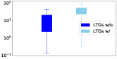
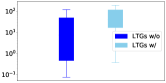
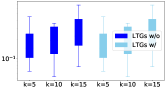
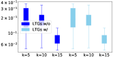
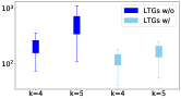
Figure 8. Time to perform lineage collection for different scenarios using LTGs.

References

- (1)
- Abiteboul et al. (1995) Serge Abiteboul, Richard Hull, and Victor Vianu. 1995. Foundations of Databases. Addison-Wesley.
- Aditya et al. (2019) Somak Aditya, Yezhou Yang, and Chitta Baral. 2019. Integrating Knowledge and Reasoning in Image Understanding. In IJCAI. 6252–6259.
- Antova et al. (2008) Lyublena Antova, Thomas Jansen, Christoph Koch, and Dan Olteanu. 2008. Fast and Simple Relational Processing of Uncertain Data. In ICDE. 983–992.
- Bach et al. (2017) Stephen H. Bach, Matthias Broecheler, Bert Huang, and Lise Getoor. 2017. Hinge-Loss Markov Random Fields and Probabilistic Soft Logic. Journal of Machine Learning Research 18 (2017), 109:1–109:67.
- Bancilhon et al. (1986) François Bancilhon, David Maier, Yehoshua Sagiv, and Jeffrey D. Ullman. 1986. Magic Sets and Other Strange Ways to Implement Logic Programs. In PODS. 1–15.
- Bárány et al. (2017) Vince Bárány, Balder ten Cate, Benny Kimelfeld, Dan Olteanu, and Zografoula Vagena. 2017. Declarative Probabilistic Programming with Datalog. ACM Trans. Database Syst. 42, 4 (2017), 22:1–22:35.
- Barceló and Pichler (2012) Pablo Barceló and Reinhard Pichler (Eds.). 2012. Datalog in Academia and Industry - Second International Workshop. Lecture Notes in Computer Science, Vol. 7494. Springer.
- Beeri and Ramakrishnan (1991) Catriel Beeri and Raghu Ramakrishnan. 1991. On the Power of Magic. Journal of Logic Programming 10 (1991), 255–299.
- Bellomarini et al. (2018) L. Bellomarini, E. Sallinger, and G. Gottlob. 2018. The Vadalog System: Datalog-based Reasoning for Knowledge Graphs. PVLDB 11, 9 (2018), 975–987.
- Benedikt et al. (2017) Michael Benedikt, George Konstantinidis, Giansalvatore Mecca, Boris Motik, Paolo Papotti, Donatello Santoro, and Efthymia Tsamoura. 2017. Benchmarking the Chase. In PODS. 37–52.
- Benedikt et al. (2018) Michael Benedikt, Boris Motik, and Efthymia Tsamoura. 2018. Goal-Driven Query Answering for Existential Rules With Equality. In AAAI. 1761–1770.
- Bizer et al. (2009) C. Bizer, J. Lehmann, G. Kobilarov, S. Auer, C. Becker, R. Cyganiak, and S. Hellman. 2009. DBpedia - A crystallization point for the Web of Data. Journal of Web Semantics 7, 3 (2009), 154–165.
- Bosselut et al. (2019) Antoine Bosselut, Hannah Rashkin, Maarten Sap, Chaitanya Malaviya, Asli Celikyilmaz, and Yejin Choi. 2019. COMET: Commonsense Transformers for Automatic Knowledge Graph Construction. In ACL. 4762–4779.
- Chandra and Merlin (1977) Ashok K. Chandra and Philip M. Merlin. 1977. Optimal Implementation of Conjunctive Queries in Relational Data Bases. In STOC. 77–90.
- Cohen et al. (2020) William W. Cohen, Fan Yang, and Kathryn Mazaitis. 2020. TensorLog: A Probabilistic Database Implemented Using Deep-Learning Infrastructure. J. Artif. Intell. Res. 67 (2020), 285–325.
- Cussens (2000) James Cussens. 2000. Stochastic Logic Programs: Sampling, Inference and Applications. In UAI. 115–122.
- Dalvi et al. (2009) Nilesh Dalvi, Christopher Ré, and Dan Suciu. 2009. Probabilistic Databases: Diamonds in the Dirt. Commun. ACM 52, 7 (2009), 86–94.
- Dalvi and Suciu (2007a) Nilesh N. Dalvi and Dan Suciu. 2007a. The dichotomy of conjunctive queries on probabilistic structures. In PODS. 293–302.
- Dalvi and Suciu (2007b) Nilesh N. Dalvi and Dan Suciu. 2007b. Efficient query evaluation on probabilistic databases. VLDB J. 16, 4 (2007), 523–544.
- Dalvi and Suciu (2012) Nilesh N. Dalvi and Dan Suciu. 2012. The dichotomy of probabilistic inference for unions of conjunctive queries. J. ACM 59, 6 (2012), 30:1–30:87.
- Dannert et al. (2021) Katrin M. Dannert, Erich Grädel, Matthias Naaf, and Val Tannen. 2021. Semiring Provenance for Fixed-Point Logic. In CSL, Vol. 183. 17:1–17:22.
- Darwiche (2004) Adnan Darwiche. 2004. New Advances in Compiling CNF to Decomposable Negation Normal Form. In ECAI. 318–322.
- Darwiche (2011) Adnan Darwiche. 2011. SDD: A New Canonical Representation of Propositional Knowledge Bases. In IJCAI. 819–826.
- De Raedt and Kimmig (2015) Luc De Raedt and Angelika Kimmig. 2015. Probabilistic (logic) programming concepts. Machine Learning 100, 1 (2015), 5–47.
- De Raedt et al. (2007) Luc De Raedt, Angelika Kimmig, and Hannu Toivonen. 2007. ProbLog: A Probabilistic Prolog and Its Application in Link Discovery. In IJCAI. 2462–2467.
- Dettmers et al. (2018) Tim Dettmers, Pasquale Minervini, Pontus Stenetorp, and Sebastian Riedel. 2018. Convolutional 2D Knowledge Graph Embeddings. In AAAI. 1811–1818.
- Deutch et al. (2018) Daniel Deutch, Amir Gilad, and Yuval Moskovitch. 2018. Efficient provenance tracking for datalog using top-k queries. VLDB Journal 27, 2 (2018), 245–269.
- Deutch et al. (2014) Daniel Deutch, Tova Milo, Sudeepa Roy, and Val Tannen. 2014. Circuits for Datalog Provenance. In ICDT. 201–212.
- Deutsch et al. (2008) A. Deutsch, A. Nash, and J. B. Remmel. 2008. The chase revisited. In PODS. 149–158.
- Domingos et al. (2008) Pedro Domingos, Stanley Kok, Daniel Lowd, Hoifung Poon, Matthew Richardson, and Parag Singla. 2008. Markov Logic. 92–117.
- Dong et al. (2014) Xin Luna Dong, Evgeniy Gabrilovich, Geremy Heitz, Wilko Horn, Ni Lao, Kevin Murphy, Thomas Strohmann, Shaohua Sun, and Wei Zhang. 2014. Knowledge Vault: A Web-Scale Approach to Probabilistic Knowledge Fusion. In KDD. 601–610.
- Dylla et al. (2013) Maximilian Dylla, Iris Miliaraki, and Martin Theobald. 2013. A Temporal-Probabilistic Database Model for Information Extraction. PVLDB 6, 14 (2013), 1810–1821.
- Dylla et al. (2013) M. Dylla, I. Miliaraki, and M. Theobald. 2013. Top-k query processing in probabilistic databases with non-materialized views. In ICDE. 122–133.
- Fierens et al. (2015) Daan Fierens, Guy Van den Broeck, Joris Renkens, Dimitar Shterionov, Bernd Gutmann, Ingo Thon, Gerda Janssens, and Luc De Raedt. 2015. Inference and learning in probabilistic logic programs using weighted Boolean formulas. Theory and Practice of Logic Programming (TPLP) 15, 3 (2015), 358–401.
- Fink et al. (2013) Robert Fink, Jiewen Huang, and Dan Olteanu. 2013. Anytime approximation in probabilistic databases. VLDB Journal 22, 6 (2013), 823–848.
- Friedman and den Broeck (2019) Tal Friedman and Guy Van den Broeck. 2019. On Constrained Open-World Probabilistic Databases. In IJCAI. 5722–5729.
- Friedman and den Broeck (2020) Tal Friedman and Guy Van den Broeck. 2020. Symbolic Querying of Vector Spaces: Probabilistic Databases Meets Relational Embeddings. In UAI. 1268–1277.
- Fuhr (1995) Norbert Fuhr. 1995. Probabilistic Datalog - A Logic For Powerful Retrieval Methods. In SIGIR. 282–290.
- Fuhr (2000) Norbert Fuhr. 2000. Probabilistic datalog: Implementing logical information retrieval for advanced applications. JASIS 51, 2 (2000), 95–110.
- Gao et al. (2019) Difei Gao, Ruiping Wang, Shiguang Shan, and Xilin Chen. 2019. From Two Graphs to N Questions: A VQA Dataset for Compositional Reasoning on Vision and Commonsense. CoRR abs/1908.02962 (2019).
- Gatterbauer and Suciu (2014) Wolfgang Gatterbauer and Dan Suciu. 2014. Oblivious Bounds on the Probability of Boolean Functions. ACM Transactions on Database Systems 39, 1 (2014).
- Grädel (1992) Erich Grädel. 1992. On transitive closure logic. In Computer Science Logic. Springer Berlin Heidelberg, 149–163.
- Green et al. (2007) Todd J. Green, Grigoris Karvounarakis, and Val Tannen. 2007. Provenance Semirings. In PODS. 31–40.
- Gribkoff and Suciu (2016) Eric Gribkoff and Dan Suciu. 2016. SlimShot: In-Database Probabilistic Inference for Knowledge Bases. PVLDB 9, 7 (2016), 552–563.
- Gribkoff et al. (2014) Eric Gribkoff, Guy Van den Broeck, and Dan Suciu. 2014. The most probable database problem. In BUDA. 1–7.
- Guo et al. (2011) Y. Guo, Z. Pan, and J. Heflin. 2011. LUBM: A Benchmark for OWL Knowledge Base Systems. Journal of Web Semantics 3, 2-3 (2011).
- Gutmann et al. (2008) Bernd Gutmann, Angelika Kimmig, Kristian Kersting, and Luc De Raedt. 2008. Parameter Learning in Probabilistic Databases: A Least Squares Approach. In Machine Learning and Knowledge Discovery in Databases. 473–488.
- Gutmann et al. (2011) Bernd Gutmann, Ingo Thon, Angelika Kimmig, Maurice Bruynooghe, and Luc De Raedt. 2011. The magic of logical inference in probabilistic programming. Theory and Practice of Logic Programming 11, 4-5 (2011), 663–680.
- Huang et al. (2021) Jiani Huang, Ziyang Li, Binghong Chen, Karan Samel, Mayur Naik, Le Song, and Xujie Si. 2021. Scallop: From Probabilistic Deductive Databases to Scalable Differentiable Reasoning. In NeurIPS. 25134–25145.
- Joshi et al. (2020) Unmesh Joshi, Ceriel J. H. Jacobs, and Jacopo Urbani. 2020. Rewrite or Not Rewrite? ML-Based Algorithm Selection for Datalog Query Answering on Knowledge Graphs. In ECAI. 792–799.
- Kaliszyk et al. (2018) Cezary Kaliszyk, Josef Urban, Henryk Michalewski, and Miroslav Olsák. 2018. Reinforcement Learning of Theorem Proving. In NeurIPS. 8836–8847.
- Khoussainova et al. (2008) Nodira Khoussainova, Magdalena Balazinska, and Dan Suciu. 2008. Probabilistic Event Extraction from RFID Data. In ICDE. 1480–1482.
- Kimmig et al. (2011) A. Kimmig, B. Demoen, L. De Raedt, V. Santos Costa, and R. Rocha. 2011. On the implementation of the probabilistic logic programming language ProbLog. Theory and Practice of Logic Programming 11, 2-3 (2011), 235–262.
- Lacroix et al. (2018) Timothée Lacroix, Nicolas Usunier, and Guillaume Obozinski. 2018. Canonical Tensor Decomposition for Knowledge Base Completion. In ICML. 2869–2878.
- Mahdisoltani et al. (2014) Farzaneh Mahdisoltani, Joanna Biega, and Fabian Suchanek. 2014. Yago3: A knowledge base from multilingual wikipedias. In CIDR.
- Manhaeve et al. (2018) Robin Manhaeve, Sebastijan Dumancic, Angelika Kimmig, Thomas Demeester, and Luc De Raedt. 2018. DeepProbLog: Neural Probabilistic Logic Programming. In NeurIPS. 3749–3759.
- Meilicke et al. (2019) Christian Meilicke, Melisachew Wudage Chekol, Daniel Ruffinelli, and Heiner Stuckenschmidt. 2019. Anytime Bottom-Up Rule Learning for Knowledge Graph Completion. In IJCAI. 3137–3143.
- Motik et al. (2015) Boris Motik, Yavor Nenov, Robert Piro, and Ian Horrocks. 2015. Handling owl:sameAs via Rewriting. In AAAI. 231–237.
- Moustafa et al. (2016) W. E. Moustafa, V. Papavasileiou, K. Yocum, and A. Deutsch. 2016. Datalography: Scaling datalog graph analytics on graph processing systems. In IEEE International Conference on Big Data. 56–65.
- Nenov et al. (2015) Yavor Nenov, Robert Piro, Boris Motik, Ian Horrocks, Zhe Wu, and Jay Banerjee. 2015. RDFox: A Highly-Scalable RDF Store. In ISWC. 3–20.
- Nitti et al. (2014) Davide Nitti, Tinne De Laet, and Luc De Raedt. 2014. Relational object tracking and learning. In ICRA. 935–942.
- Olteanu et al. (2010) Dan Olteanu, Jiewen Huang, and Christoph Koch. 2010. Approximate confidence computation in probabilistic databases. In ICDE. 145–156.
- Pipatsrisawat and Darwiche (2008) Knot Pipatsrisawat and Adnan Darwiche. 2008. New Compilation Languages Based on Structured Decomposability. In AAAI. 517–522.
- Poole (1992) David Poole. 1992. Logic Programming, Abduction and Probability. In FGCS. 530–538.
- Poole (2008) David Poole. 2008. The Independent Choice Logic and Beyond. In Probabilistic Inductive Logic Programming. 222–243.
- Rahtz et al. (2011) Sebastian Rahtz, Alexander Dutton, Donna Kurtz, Graham Klyne, Andrew Zisserman, and Relja Arandjelovic. 2011. CLAROS—Collaborating on Delivering the Future of the Past. In DH. Stanford University Library, 355–357.
- Ramusat et al. (2021) Yann Ramusat, Silviu Maniu, and Pierre Senellart. 2021. A Practical Dynamic Programming Approach to Datalog Provenance Computation. CoRR abs/2112.01132 (2021).
- Ré and Suciu (2008) Christopher Ré and Dan Suciu. 2008. Approximate Lineage for Probabilistic Databases. In VLDB. 797–808.
- Renkens et al. (2014) Joris Renkens, Angelika Kimmig, Guy Van den Broeck, and Luc De Raedt. 2014. Explanation-Based Approximate Weighted Model Counting for Probabilistic Logics. In AAAI. 2490–2496.
- Renkens et al. (2012) Joris Renkens, Guy Van den Broeck, and Siegfried Nijssen. 2012. k-Optimal: A Novel Approximate Inference Algorithm for ProbLog. In Inductive Logic Programming. 33–38.
- Richardson and Domingos (2006) Matthew Richardson and Pedro M. Domingos. 2006. Markov logic networks. Machine Learning 62, 1-2 (2006), 107–136.
- Roth (1996) Dan Roth. 1996. On the Hardness of Approximate Reasoning. Artif. Intell. 82, 1–2 (1996), 273–302.
- Sato (1995) Taisuke Sato. 1995. A statistical learning method for logic programs with distribution semantics. In ICLP. 715–729.
- Schoenfisch and Stuckenschmidt (2017) Joerg Schoenfisch and Heiner Stuckenschmidt. 2017. Analyzing real-world SPARQL queries and ontology-based data access in the context of probabilistic data. Int. J. Approx. Reasoning 90 (2017), 374–388.
- Sen et al. (2009) Prithviraj Sen, Amol Deshpande, and Lise Getoor. 2009. PrDB: Managing and Exploiting Rich Correlations in Probabilistic Databases. The VLDB Journal 18, 5 (2009), 1065–1090.
- Suciu et al. (2011) Dan Suciu, Dan Olteanu, Christopher Ré, and Christoph Koch. 2011. Probabilistic Databases. Morgan & Claypool Publishers.
- Tsamoura et al. (2021a) Efthymia Tsamoura, David Carral, Enrico Malizia, and Jacopo Urbani. 2021a. Materializing Knowledge Bases via Trigger Graphs. PVLDB 14, 6 (2021), 943–956.
- Tsamoura et al. (2020) Efthymia Tsamoura, Victor Gutiérrez-Basulto, and Angelika Kimmig. 2020. Beyond the Grounding Bottleneck: Datalog Techniques for Inference in Probabilistic Logic Programs. In AAAI. 10284–10291.
- Tsamoura et al. (2021b) Efthymia Tsamoura, Timothy Hospedales, and Loizos Michael. 2021b. Neural-Symbolic Integration: A Compositional Perspective. In AAAI. 5051–5060.
- Urbani et al. (2016) Jacopo Urbani, Ceriel Jacobs, and Markus Krötzsch. 2016. Column-Oriented Datalog Materialization for Large Knowledge Graphs. In AAAI. 258–264.
- Valiant (1979) Leslie G. Valiant. 1979. The Complexity of Enumeration and Reliability Problems. SIAM J. Comput. 8, 3 (1979), 410–421.
- van Bremen et al. (2019) Timothy van Bremen, Anton Dries, and Jean Christoph Jung. 2019. Ontology-Mediated Queries over Probabilistic Data via Probabilistic Logic Programming. In CIKM. 2437–2440.
- Van den Broeck et al. (2014) Guy Van den Broeck, Wannes Meert, and Adnan Darwiche. 2014. Skolemization for Weighted First-Order Model Counting. In KR. 111–120.
- Van den Heuvel et al. (2019) Maarten Van den Heuvel, Peter Ivanov, Wolfgang Gatterbauer, Floris Geerts, and Martin Theobald. 2019. Anytime Approximation in Probabilistic Databases via Scaled Dissociations. In SIGMOD. 1295–1312.
- Vlasselaer et al. (2015) Jonas Vlasselaer, Guy Van den Broeck, Angelika Kimmig, Wannes Meert, and Luc De Raedt. 2015. Anytime inference in probabilistic logic programs with Tp-compilation. In IJCAI. 1852–1858.
- Vlasselaer et al. (2016) Jonas Vlasselaer, Guy Van den Broeck, Angelika Kimmig, Wannes Meert, and Luc De Raedt. 2016. TP-Compilation for inference in probabilistic logic programs. International Journal of Approximate Reasoning 78 (2016), 15 – 32.
- Wu et al. (2015) Sen Wu, Ce Zhang, Feiran Wang, and Christopher Ré. 2015. Incremental Knowledge Base Construction Using DeepDive. CoRR abs/1502.00731 (2015).
- Wu et al. (2012) Wentao Wu, Hongsong Li, Haixun Wang, and Kenny Q. Zhu. 2012. Probase: A Probabilistic Taxonomy for Text Understanding. In SIGMOD. 481–492.
- Zhu et al. (2014) Yuke Zhu, Alireza Fathi, and Li Fei-Fei. 2014. Reasoning about Object Affordances in a Knowledge Base Representation. In ECCV. 408–424.