Limiting propulsion of ionic microswimmers

Abstract

Self-propulsion of catalytic Janus swimmers in electrolyte solutions is induced by inhomogeneous ion release from their surface. Here, we consider the experimentally relevant cases of particles which emit only one type of ions (type I) or equal fluxes of cations and anions (type II). In the limit of a thin electrostatic diffuse layer we derive a nonlinear outer solution for the electric field and concentrations of active (i.e. released from the surface) and passive ionic species. We show that for swimmers of type I both the maximum ion flux and propulsion velocity are constrained. This suggests that the propulsion of Janus swimmers can be optimized by tuning the concentration of active ions.

I Introduction

Catalytic Janus swimmers have drawn a considerable interest during last decadesmoran2017 ; dey2017 ; asmolov2022COCIS because of their ability to move autonomously. The potential applications include drug delivery, lab-on-a-chip devices and nano-roboticshu2020micro . The self-propulsion mechanism of ionic swimmers is based on an inhomogeneous ion release at the particle surface. Ion diffusion induces concentration gradient and electric fieldgolestanian2005propulsion .

Despite the variety of catalytic reactions, two main models for ionic flux are acceptedasmolov2022COCIS ; Wang2020practical ; peng2022generic (see Fig. 1): only one type of ions is released (Type I) and equal fluxes of cations and anions (Type II). The classical examples of the first type include bimetallicpaxton2004 and metallic-insulator howse2007 Janus particles. As a result of hydrogen peroxide decomposition on the catalytic particle side, protons are released into solution and then are adsorbed on the non-catalytic side. The ionic flux for the second type can be generated by the salt dissolution in watermcdermott2012 , enzyme-enhanced decomposition of organic compoundsdey2015micromotors ; patino2018fundamental or by photochemical reactionszhou2018 .

Charged particle immersed in an electrolyte solution is surrounded by an electric diffuse layer (EDL), where charge imbalance is large and the electric field is strong. Concentration of ionic species, electric potential and fluid flow near catalytic swimmers are governed by a system of the Nernst-Planck, Poisson and Stokes equations. The EDL is thin for swimmers of micron size, and the method of matched asymptotic expansions is usually applied for the theoretical description of self-propulsionprieve.dc:1984 ; anderson.jl:1989 ; golestanian2007 . The EDL effect appears macroscopically as a slip velocity at the particle surface. The electric field in the outer region (at distances of the order of the particle size) is not zero due to ion diffusion and small charge imbalance and can effect on the slip velocitynourhani2015 ; asmolov2022self . The analytical solutions in the outer region has been obtained for the swimmer of Type Inourhani2015 ; ibrahim2017 under the assumption that field disturbances are small and the Nernst-Planck equations can be linearized.

Recently, we have proposedasmolov2022self ; asmolov2022MDPI non-linear analytical solutions to Nernst-Planck and Poisson equations for the cases when bulk electrolyte contains active (released from the swimmer surface) ions only. However, the self-propulsion in experiments is carried out in media containing both active and passive ions. The addition of passive salt reduces the swimmer velocitymoran2017 ; ibrahim2017 ; arque2020ionic . In the present paper, we extend our previous solutions to include the effect of passive ions in the bulk. We obtain the analytical solutions in the outer region for both swimmer types and all ionic species. The depletion of active ions arise for the swimmer of Type I near an adsorbing particle side. This imposes a constraint on the maximum swimmer velocity.

Our paper is organized as follows. The governing equations are formulated in Sec. II. Their solution at distances of the order of particle size (outer region) is given in Sec. III. Our numerical results for concentrations and for the limiting particle velocity are presented in Sec. IV and are summarized in Sec. V.

II Governing equations

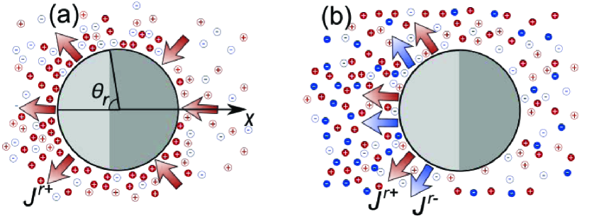
Figure 1: Two types of ionic swimmers. (a) Type I releases cations only at the active side and adsorb them at the other side. (b) Type II releases both cations and anions at the active side.

We consider an 1:1 aqueous electrolyte solution with the bulk ion concentration $c_{\infty}.$ It includes passive salt ions with dimensionless concentrations $C^{s\pm}\left(\mathbf{r}\right)\$(scaled by $c_{\infty})$ and ions which are released from the particle surface with concentrations $C^{r\pm}\left(\mathbf{r}\right)$. Here the upper (lower) sign corresponds to the positive (negative) ions. The Peclet number is assumed to be small, so that the convective fluxes are ignored, and the ion fluxes are governed by dimensionless Nernst-Planck equations

$$\nabla\cdot\mathbf{J}^{i}=0,$$ (1)

$$\mathbf{J}^{i}=-\nabla C^{i}\mp C^{i}\nabla\Phi.$$ (2)

Here $i=r\pm,$ $s\pm,$ the electric potential $\Phi$ is scaled by $k_{B}T/e,$ where $e$ is the elementary positive charge, $k_{B}$ is the Boltzmann constant, $T$ is the temperature of the system, and coordinates are scaled by the particle size $a.$

Unequal distributions of oppositely charged ions generate an electric field, governed by the Poisson equation for the electric potential,

$$\Delta\Phi=\lambda^{-2}\frac{C^{s+}+C^{r+}-C^{s-}-C^{r-}}{2},$$ (3)

where the dimensionless parameter $\lambda=\left(\kappa a\right)^{-1}$ is the ratio of the Debye length $\kappa^{-1}=\left(8\pi e^{2}c_{\infty}/\epsilon k_{B}T\right)^{-1/2}$ to the particle size, $\epsilon$ is the permittivity of the fluid. We consider large particles with a thin electric double layer (EDL), i.e. $\lambda\ll 1,$ and construct the asymptotic solution using the method of matched expansions in two regions with different lengthscales. The lengthscale of the outer region is the particle size $a$ and that for the inner region is the Debye length $\kappa^{-1}$.

The boundary conditions at the particle surface $S$ (defined by $\mathbf{r}=\mathbf{r}_{s}$) read,

$$\mathbf{r}\in S:\ \mathbf{J}^{r+}\cdot\mathbf{n}=-\mathrm{Da}j^{+}\left(\mathbf{r}_{s}\right),$$ (4)

$$\mathbf{J}^{r-}\cdot\mathbf{n}=-\mathrm{Da}j^{-}\left(\mathbf{r}_{s}\right),$$ (5)

$$\mathbf{J}^{s\pm}\cdot\mathbf{n}=0,$$ (6)

$$\ \Phi=\phi_{s}\left(\mathbf{r}_{s}\right),$$ (7)

$$\mathrm{Da}=\frac{Ja}{c_{\infty}D^{r+}},$$ (8)

where $\mathrm{Da}$ is the Damköhler number and $J$ is the average module of dimensional flux of released cations. The first two conditions define the surface fluxes of active ions, and the third one the zero fluxes for passive ions. The functions $j^{\pm}\left(\mathbf{r}_{s}\right)$ characterize dimensionless inhomogeneous ion productions at the particle surface. Because of definition (8) the cation flux satisfies the condition

$$\frac{1}{S}\int_{S_{p}}\left|j^{+}\right|dS=1.$$ (9)

The net flux for the swimmers of Type I should vanish in a steady state:

$$\int_{S_{p}}j^{+}dS=0.$$ (10)

The boundary condition (7) sets the surface potential $\phi_{s}$ which are assumed to be constant.

Boundary conditions at infinity are,

$$r\rightarrow\infty:\ C^{s\pm}=C_{\infty}^{s\pm},\ C^{r\pm}=C_{\infty}^{r\pm},\ \Phi=0.$$ (11)

The bulk electrolyte solution is electroneutral, so that

$$C_{\infty}^{s+}+C_{\infty}^{r+}=C_{\infty}^{s-}+C_{\infty}^{r-}=1.$$

The fluid flow satisfies the Stokes equations,

$$\mathbf{\nabla\cdot v}=0\mathbf{,\quad}\Delta\mathbf{v}-\mathbf{\nabla}p=\mathbf{f}.$$ (12)

Here $\mathbf{v}$ and $p$ are the dimensionless fluid velocity and pressure (scaled by $\dfrac{\epsilon k_{B}^{2}T^{2}}{4\pi\eta e^{2}a}$ and $\dfrac{\epsilon k_{B}^{2}T^{2}}{4\pi e^{2}a^{2}}$), $\eta$ the viscosity and $\mathbf{f}=-\Delta\Phi\mathbf{\nabla}\Phi$ is the electrostatic body force.

III Theory

In this section we present the solution of the system (1)-(8) in the outer region with the lengthscale $a.$ Since $\lambda\ll 1,$ the leading-order solution of (3) in the outer region is

$$C^{s+}+C^{r+}=C^{s-}+C^{r-}=C\left(\mathbf{r}\right),$$ (13)

i.e. the electroneutrality holds to $O\left(\lambda^{2}\right).$ However, one should take into account the small charge $C^{s+}+C^{r+}-C^{s-}-C^{r-}=O\left(\lambda^{2}\right)$, since it induces a finite potential difference in the outer region. We sum up the equations (1) for positive and negative ions, and the system then becomes

$$\Delta C+\nabla\cdot\left(C\nabla\Phi\right) = 0,$$ (14)

$$\Delta C-\nabla\cdot\left(C\nabla\Phi\right) = 0.$$ (15)

Summing up and subtracting equations (14) and (15) we obtainnourhani2015 ; ibrahim2017 ; asmolov2022MDPI :

$$\Delta C = 0,$$ (16)

$$\nabla\cdot\left(C\nabla\Phi\right) = 0.$$ (17)

Likewise, by calculating the sum and difference of Eqs.(4), (5) and (6) we derive the boundary conditions to (16) and (17),

$$\mathbf{r}\in S:\ \mathbf{\nabla}C\cdot\mathbf{n}=-\frac{\mathrm{Da}}{2}\left(j^{+}+j^{-}\right),$$ (18)

$$C\mathbf{\nabla}\Phi\cdot\mathbf{n}=-\frac{\mathrm{Da}}{2}\left(j^{+}-j^{-}\right).$$ (19)

Solution of Laplace equation (16) makes it possible to find the net ion concentrations $C$. However, the solution of a non-linear equation for the electric potential (17) is generally not straightforward. We consider here the case of the constant ratio of the surface fluxes,

$$j^{-}\left(\mathbf{r}_{s}\right)/j^{+}\left(\mathbf{r}_{s}\right)=\alpha=\text{const}.$$ (20)

The condition is valid for the two swimmer type: $\alpha=0$ for the Type I (cations are released only) and $\alpha=D^{r+}/D^{r-}$ for the Type II. The solution of (17) satisfying the boundary conditions (11) and (19) isasmolov2022MDPI

$$\Phi=-\beta\ln\left(C\right),$$ (21)

$$\beta=\dfrac{\alpha-1}{\alpha+1}.$$ (22)

The above dimensionless parameter is limited, namely $\left|\beta\right|\leq 1.$

To find the concentrations $C^{i}$ we do not need to solve the system (1)-(6). The boundary fluxes for passive ions $C^{s\pm}$ are zero, so their fields obey the Boltzmann distribution,

$$C^{s\pm}=C_{\infty}^{s\pm}\exp\left(\mp\Phi\right)=C_{\infty}^{s\pm}C^{\pm\beta}.$$ (23)

Once $C$ and $C^{s\pm}$ are known we can also determine the distributions of active ions from Eqs. (13), (23):

$$C^{r+} = C-C^{s+}=C-C_{\infty}^{s+}C^{\beta},$$ (24)

$$C^{r-} = C-C^{s-}=C-C_{\infty}^{s-}C^{-\beta}.$$ (25)

Thus, we obtain concentrations of all ionic species in the outer region for arbitrary $\mathrm{Da}$ and $j^{\pm}\left(\mathbf{r}_{s}\right).$ This is one of the main results of our work. However, physically reasonable results may not be found for any boundary conditions. The restriction comes from the condition that the concentrations may not be negative for all $\mathbf{r}$ and $i,$

$$C^{i}\left(\mathbf{r}\right)\geq 0.$$ (26)

This implies physical constraints on $\mathrm{Da}$ for given $C_{\infty}^{i}$ and $j^{\pm}\left(\mathbf{r}_{s}\right)$. When the normal gradient $\mathbf{\nabla}C\cdot\mathbf{n}$ is negative over the entire particle surface, i.e. the net flux of released ions $j^{+}\left(\mathbf{r}_{s}\right)+j^{-}\left(\mathbf{r}_{s}\right)$ is always positive as for the Type II, the solution of (16) satisfies the condition $C\geq 1$ for any $\mathbf{r,}$ i.e. the net concentration exceeds the bulk value. This means that the concentration of released ions (Eqs. (24), (25)) is always positive since $C_{\infty}^{s\pm}\leq 1.$ The opposite situation takes place for the Type I when ions are adsorbed at some surface portion, where the surface flux is negative and $\mathbf{\nabla}C\cdot\mathbf{n}$ is positive. Then we may obtain physically impossible solution $C\leq 0,$ when $\mathrm{Da}$ is large enough. Moreover, negative solutions for active ions can follow from Eqs. (24), (25) even at smaller $\mathrm{Da}$ (see Sec. IV). Therefore, there is a limiting value $\mathrm{Da}_{\mathrm{max}}$ for which the minimum concentration $C_{\infty}^{r\pm}=0.$

Solution in the inner region expresses the slip velocity $\mathbf{v}_{s}$ at the outer edge of the EDLprieve.dc:1984 ; anderson.jl:1989

$$\mathbf{v}_{s}=\psi\nabla_{s}\Phi_{s}+4\nabla_{s}(\ln C_{s})\ln\left[\cosh\left(\frac{\psi}{4}\right)\right],$$ (27)

$$\psi=\phi_{s}-\Phi_{s},\quad\Phi_{s}=\Phi\left(\mathbf{r}_{s}\right),\quad C_{s}=C\left(\mathbf{r}_{s}\right).$$

Here $\nabla_{s}$ is the gradient operator along the particle surface, the first and the second terms in Eq.(27) are associated with electro- and diffusio-osmotic flows, respectively, $\psi$ is the potential drop in the inner region, $\Phi_{s}$ and $C_{s}$ are the outer potential and the concentration at the dividing surface between the inner and outer regions.

The velocity of a freely moving in the $x-$direction particle can be determined by using the reciprocal theoremteubner1982

$$v_{p}=-\frac{1}{6\pi}\int_{V_{f}}\mathbf{f}\cdot\left(\mathbf{v}_{1}-\mathbf{e}_{x}\right)dV.$$ (28)

The integral is evaluated over the whole fluid volume $V_{f}$ and $\mathbf{v}_{1}\left(\mathbf{r}\right)$ represents the velocity field for the particle of the same shape that translates with the velocity $\mathbf{e}_{x}$ in a stagnant fluid. The velocity can be presented as a superimposition of the contributions of the outer and inner regionsasmolov2022self ,

$$v_{p}=v_{po}+v_{pi},$$ (29)

$$v_{po}=-\frac{\beta^{2}}{6\pi}\int_{V_{f}}\frac{\left(\mathbf{\nabla}C\right)^{2}\mathbf{\nabla}C\cdot\left(\mathbf{v}_{1}-\mathbf{e}_{x}\right)}{C^{3}}dV,$$ (30)

$$v_{pi}=-\frac{1}{S}\int_{S_{p}}\left(\mathbf{v}_{s}\cdot\mathbf{e}_{x}\right)dS.$$ (31)

Equations (27)-(31) do not include the concentrations of each ionic species, but only the net value $C.$ Hence, the velocity is independent of $C_{\infty}^{s+}$ provided $\mathrm{Da}<\mathrm{Da}_{\mathrm{max}}\left(C_{\infty}^{s+}\right).$

When the Damköhler number is small, the concentration and potential fields are slightly disturbed in the outer region, $C=1+O\left(\mathrm{Da}\right)\mathrm{,\ }\Phi=O\left(\mathrm{Da}\right),$ $\psi\simeq\phi_{s}$ as $\mathrm{Da}\ll 1.$ Contribution of the outer region to the velocity is $O\left(\mathrm{Da}^{3}\right)$ and can be neglected, since the integrand in Eq. (30) is proportional to $\left(\mathbf{\nabla}C\right)^{3}$. Then the dominant contribution of the order of $\mathrm{Da}$ comes from the inner region (31) with the linearized slip velocity:

$$\mathbf{v}_{s}=\phi_{s}\nabla_{s}\Phi_{s}+4\nabla_{s}C_{s}\ln\left[\cosh\left(\frac{\phi_{s}}{4}\right)\right]=O\left(\mathrm{Da}\right).$$ (32)

Below we show that this linear solution approximates well the exact results up to $\mathrm{Da}\sim 1.$

IV Results and discussion

We consider spherical particle with symmetric ion release with respect to $x-$ axis, so that $j^{\pm}$ depends on azimuthal angle $\theta$ only. The boundary condition (18) is rewritten as

$$r=1:\ \partial_{r}C=-\frac{\mathrm{Da}}{2}\left(j^{+}+j^{-}\right).$$ (33)

We use the spherical coordinate system to solve Eq. (16) with the boundary conditions (33) and present the solution in terms of Legendre polynomials $P_{n}\left(\cos\theta\right)$,

$$C=1+\frac{\mathrm{Da}}{2}\xi\left(r,\theta\right),$$ (34)

$$\xi = \sum_{n=0}^{\infty}\frac{j_{n}}{n+1}P_{n}\left(\cos\theta\right)r^{-n-1},$$ (35)

$$j_{n} = \left(n+\frac{1}{2}\right)\int_{0}^{\pi}\left(j^{+}+j^{-}\right)P_{n}\sin\theta d\theta.$$ (36)

We model inhomogeneous distributions $j^{+}\left(\theta\right),j^{-}\left(\theta\right)$ by piecewise constant functions, i.e. the ions are released from the surface for $\theta\leq\theta_{r}.$ At the other sphere side, $\theta_{r}<\theta\leq\pi,$ cations are adsorbed for the swimmer Type I (see Fig. 1(a)), and the fluxes are zero for the Type II (see Fig. 1(b)). Then the surface flux distributions satisfying conditions (9) and (10) are

$$\begin{array}[]{cc}0\leq\theta\leq\theta_{r}:&j^{+}=\frac{1}{2\left(1+\cos\theta_{r}\right)}<0,\ j^{-}=0,\\ \theta_{r}<\theta\leq\pi:&j^{+}=-\frac{1}{2\left(1-\cos\theta_{r}\right)}>0,\ j^{-}=0,\end{array}$$ (37)

for the first type, and

$$\begin{array}[]{cc}0\leq\theta\leq\theta_{r}:&j^{+}=j^{-}/\alpha=\frac{1}{\left(1+\cos\theta_{r}\right)}>0,\\ \theta_{r}<\theta\leq\pi:&j^{+}=j^{-}=0,\end{array}$$ (38)

for the second one.

We evaluate numerically the integrals in Eq. (36) to obtain a reduced ion concentration $\xi\left(r,\theta\right)$ with the surface fluxes (37) and (38) on a uniform grid in $\theta$ with $N_{\theta}=200.$ To evaluate the particle velocity we calculate the surface integral in Eq. (31), and the volume integral in Eq. (30) using the same grid in $\theta$ and a non-uniform grid in $r$ (with a grid step varying as $r^{2}$) with $N_{r}=100$ nodes and a cut-off radius $R_{out}=100$. Figure 2$\left(a\right)$ shows the functions $\xi_{s}\left(\theta\right)=\xi\left(1,\theta\right)$ for the swimmer of the Type I with $\beta=-1$ (solid and dashed-dotted lines) and Type II with $\beta=-0.5,\ \alpha=D^{r+}/D^{r-}=1/3$ (dashed and dotted lines). The functions decay with $\theta$, i.e. the ion concentration is always greater at the catalytic section where ions are released. For the Type II, $\xi_{s}>0$ for any angle $\theta_{r}$ over the entire surface, so that $C\geq 1$ (see Eq. (34)), i.e. the net concentration is always greater than the bulk value. In contrast, for the Type I, $\xi_{s}\left(\theta\right)$ changes the sign so that $C_{s}<1$ at the rear sphere side where the ions are adsorbed. We obtain from Eq. (34) non-physical values $C_{s}<0$ when $\mathrm{Da>Da}_{\mathrm{max}}=-2/\xi_{\mathrm{min}}$ where $\xi_{\mathrm{min}}=\xi\left(1,0\right)<0$ is the absolute minimum of the function $\xi$ attained at the rear sphere pole. The minimum $\xi_{\mathrm{min}}$ grows and the limiting Damköhler number decreases with $\theta_{r}$ (smaller area of cation adsorption).

The limiting value of $\mathrm{Da}$ becomes even smaller when we take into account the condition that the concentrations of all ionic species should also be positive. We evaluate $C^{i}$ by using Eqs. (23)-(25) and present the results in Fig. 2$\left(b,c\right).$ For the Type II, Eqs. (23)-(25) predict positive concentrations for all species (see Fig. 2$\left(c\right))$ as $C\geq 1,$ $C_{\infty}^{s+}\leq 1,\ \left|\beta\right|\leq 1,$ so that there is no limitation on $\mathrm{Da.}$ The concentrations of passive ions (dashed-dotted and dotted lines) are rather small, while those for the released ions (solid and dashed lines) are large and surpass the bulk value $C_{\infty}^{r+}=0.7.$ Another behavior can be viewed in Fig. 2$\left(b\right)$ for the Type I. The concentration of released cations (solid line) is close to zero at $\theta=\pi.$ Therefore, the Figure illustrates the limiting regime which is attained at $\mathrm{Da}_{\mathrm{max}}\simeq 6$ for given $C_{\infty}^{r+}$ and $j^{+}\left(\theta\right).$ Greater $\mathrm{Da}$ is impossible since Eq. (25) gives $C^{r+}<0.$ We note that $C_{s}^{r+}\left(\theta\right)$ (solid line) decreases significantly along the sphere surface while the concentration of passive cations $C_{s}^{s+}\left(\theta\right)$ (dash-dotted line) grows, so that the variation of the net concentration remains not too large. Thus the presence of passive salt reduces the limiting $\mathrm{Da.}$

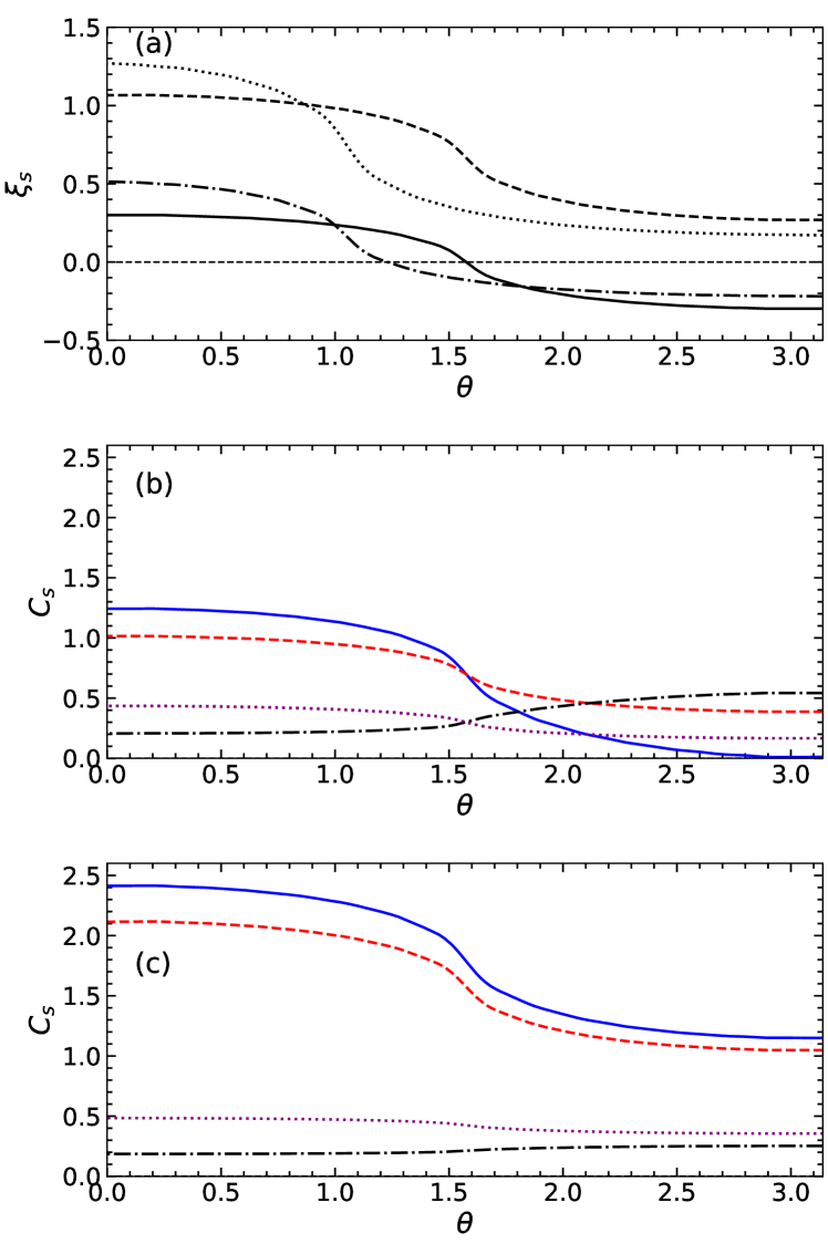
Figure 2: (a) Reduced ion concentration at the particle surface as a function of $\theta$. Solid and dashed-dotted lines correspond to the swimmer Type I with $\theta_{r}=\pi/2$ and $\theta_{r}=\pi/3$, respectively, dashed and dotted lines to the Type II, $\theta_{r}=\pi/2$ and $\theta_{r}=\pi/3$. Concentrations of ion species for swimmers of (b) the Type I and (c) Type II calculated using $\theta_{r}=\pi/2$, $\mathrm{Da}=3$ and $C_{\infty}^{s+}=0.3$. Solid and dashed lines are concentrations of released cations and anions, respectively, dashed-dotted and dotted lines are concentrations of salt cations and anions.

Condition $C^{r+}\geq 0$ can be reformulated as the limitations of the minimum bulk value or of the maximum Damköhler number. Equation (24) with $\beta=-1$ reads

$$C^{r+}=C-C_{\infty}^{s+}/C\geq 0.$$ (39)

Then by using (34) we obtain

$$C_{\infty}^{s+}\leq C_{\min}^{2}=\left(1+\frac{\mathrm{Da}}{2}\xi_{\mathrm{min}}\right)^{2},\ C_{\infty}^{r+}\geq 1-C_{\min}^{2}>0,$$ (40)

or equivalently,

$$\mathrm{Da}<\mathrm{Da}_{\mathrm{max}}=2\frac{\sqrt{C_{\infty}^{s+}}-1}{\xi_{\mathrm{min}}}.$$ (41)

The maximum Damköhler number depend only on the salt concentration $C_{\infty}^{s+}$ and the angle $\theta_{r}$. Figure 3$\left(a,b\right)$ shows $\mathrm{Da}_{\mathrm{max}}$ as the functions of the two parameters. It decreases with $\theta_{r}$ and with $C_{\infty}^{s+}.$ The active cations cannot released on the catalytic surface ($\mathrm{Da}_{\mathrm{max}}\rightarrow 0$ and $v_{p}\rightarrow 0)$ when they are absent in the bulk, $C_{\infty}^{r+}\rightarrow 0,$ or when the area of cation adsorption tends to zero $\left(\theta_{r}\rightarrow\pi\right).$

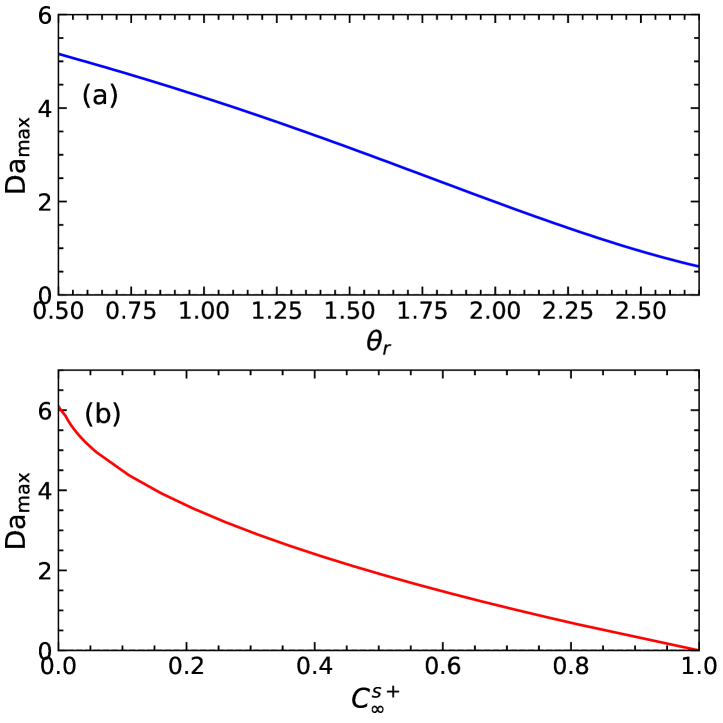
Figure 3: Limiting Damköhler number calculated as functions (a) of $\theta_{r}$ for $C_{\infty}^{s+}=0.3$ and (b) of $C_{\infty}^{s+}$ for $\theta_{r}=\pi/2$.

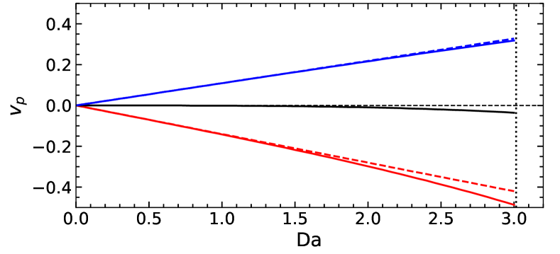
Figure 4: Particle velocities calculated using $\phi_{s}=-1$, $0$, $1$ (from top to bottom), $\theta_{r}=\pi/2$, $C_{\infty}^{s+}=0.3$ as functions of $\mathrm{Da}$. Solid curves are the total velocities $v_{pi}+v_{po}$, dashed lines correspond to the linear solution (32), dotted line is the limiting Damköhler number.

The particle velocity $v_{p}$ depends on three dimensionless parameter, $\mathrm{Da,}$ $\phi_{s},$ $\theta_{r}.$ Equations (27)-(29) do not include the concentrations of each ionic species, but only the net value $C,$ so the velocity remains the same for any $C_{\infty}^{s+}$ when $\mathrm{Da}<\mathrm{Da}_{\mathrm{max}}\left(C_{\infty}^{s+},\theta_{r}\right).$ We evaluated $v_{p}$ earlier for the swimmer Type IIasmolov2022self (see also Fig. 4 in asmolov2022COCIS ). $\mathrm{Da}$ can be arbitrary in this case, and $v_{p}$ grows logarithmically as $\mathrm{Da}\rightarrow\infty.$

We show the particle velocity for the swimmer Type I in Fig. 4 as function of the Damköhler number for different $\phi_{s}.$ The velocity of an uncharged particle $\left(\phi_{s}=0\right)$ is very small, and at finite $\phi_{s}$ and $\mathrm{Da,}$ it is close to the predictions of the linear solution (32). The maximum velocity, that is reached at $\mathrm{Da}=\mathrm{Da}_{\mathrm{max}}\left(C_{\infty}^{s+},\theta_{r}\right),$ strongly depends on $C_{\infty}^{s+}$.

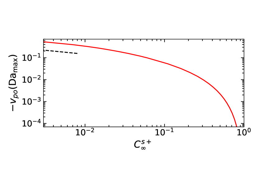
Figure 5: The contribution of the outer region to the particle velocity $v_{po}$ calculated for $\mathrm{Da}=\mathrm{Da}_{\mathrm{max}}$ and $\theta_{r}=\pi/2$ (solid line). Dashed line is the power function with the exponent $-0.355$.

We further study the dependences of the maximum particle velocity $v_{p}\left(\mathrm{Da}_{\mathrm{max}}\right)$ on $C_{\infty}^{s+},$ $\theta_{r}$ and $\phi_{s},$ and evaluate separately the contributions of the outer and the inner regions, $v_{po}$ and $v_{pi}$. The velocity $v_{po}$ is shown in Fig.  5 as the function of the salt concentration. It is negative for any $C_{\infty}^{s+},$ and is extremely small at finite salt concentration, but its magnitude grows infinitely like $\left(C_{\infty}^{s+}\right)^{-0.355}$ (dashed line) as $C_{\infty}^{s+}\rightarrow 0$. The reason is that the net ion concentration $C\left(\mathbf{r}\right)=C^{r+}+C^{s+}$ is small near the rear sphere pole in this case since both $C^{r+}$ and $C^{s+}\$tend to zero, while the gradient $\mathbf{\nabla}C$ is finite. As a result the integrand in (30) tends to infinity.

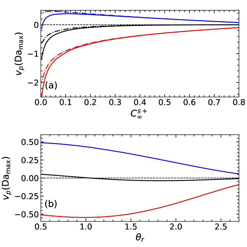
Figure 6: Limiting velocities (solid lines) as functions of (a) $C_{\infty}^{r+}$ for $\theta_{r}=\pi/2$ and (b) of $\theta_{r}$ for $C_{\infty}^{s+}=0.3$. Dashed-dotted lines correspond to the contributions of the inner region $v_{pi}$.

We show the contribution of the inner region $v_{pi}$ evaluated by using Eqs. (31), (27) and the total particle velocity $v_{p}=v_{po}+v_{pi}$ in Fig. 6. The velocity $v_{pi}$ is dominant while $v_{po}$ is negligible at finite salt concentration $C_{\infty}^{s+}$ and any $\phi_{s}.$ Up to $C_{\infty}^{s+}\simeq 0.4,$ the velocity $v_{pi}$ is nearly linear in $C_{\infty}^{r+}$ (see Fig. 6(a)), but at small $C_{\infty}^{s+}$ it grows infinitely, similar to $v_{po}$. The origin of the singularities for the two contributions is the same: $C\rightarrow 0$ near the rear pole in the limit $C_{\infty}^{s+}\rightarrow 0,$ $\mathrm{Da}\rightarrow\mathrm{Da}_{\mathrm{max}}.$ However, the singularity for $v_{pi}$ is weaker than that for $v_{po}.$ The reason is that the singularity of the slip velocity (Eq. (27)) in the integrand of (31) is weaker (proportional to $C^{-1})$ than that of the integrand in Eq. (30) for $v_{po}$ (proportional to $C^{-3}).$ The contribution of the outer region becomes dominant at very small $C_{\infty}^{s+}$, and the total velocity is negative for any $\phi_{s}.$ The maximum particle velocity decays with the angle $\theta_{r}$ i.e. with the area of the catalytic zone (see Fig. 6(b)).

V Conclusion

We have developed a theory of a self-propulsion of catalytic ionic swimmers in a media containing both active (released from the swimmer surface) and passive salt ions. The theory have involved the two types of swimmers, which release only one type of ions (Type I) or equal fluxes of cations and anions (Type II). In the limit of a thin EDL, we have derived the analytic solution for the concentrations of all ionic species at distances comparable to the particle size (outer region). For the swimmer of Type I, the constraint on the maximum Damköhler number $\mathrm{Da}_{\mathrm{max}}$ follows from the depletion of active ions near the adsorbing particle side (their concentration should be positive). $\mathrm{Da}_{\mathrm{max}}$ decreases with the salt concentration $C_{\infty}^{s+}$ but increases with the area of adsorbing part. The particle propulsion velocity grows infinitely when $\mathrm{Da}\rightarrow\mathrm{Da}_{\mathrm{max}},\ C_{\infty}^{s+}\rightarrow 0.$

DATA AVAILABILITY

The data that support the findings of this study are available within the article.

References

- [1] J. L. Moran and J. D. Posner. Phoretic self-propulsion. Annu. Rev. Fluid Mech., 49:511–540, 2017.
- [2] K. K. Dey and A. Sen. Chemically propelled molecules and machines. J. Am. Chem. Soc., 139(23):7666–7676, 2017.
- [3] T. V. Nizkaya, E. S. Asmolov, and O. I. Vinogradova. Theoretical modeling of catalytic self-propulsion. Curr. Opin. Colloid Interface Sci., 62:101637, 2022.
- [4] M. Hu, X. Ge, X. Chen, W. Mao, X. Qian, and W.-E. Yuan. Micro/nanorobot: A promising targeted drug delivery system. Pharmaceutics, 12(7):665, 2020.
- [5] R. Golestanian, T. B. Liverpool, and A. Ajdari. Propulsion of a molecular machine by asymmetric distribution of reaction products. Phys. Rev. Lett., 94(22):220801, 2005.
- [6] W. Wang, X. Lv, J. L. Moran, S. Duan, and C. Zhou. A practical guide to active colloids: choosing synthetic model systems for soft matter physics research. Soft Matter, 16(16):3846–3868, 2020.
- [7] Y. Peng, P. Xu, S. Duan, J. Liu, J. L. Moran, and W. Wang. Generic rules for distinguishing autophoretic colloidal motors. Angew. Chem., 134(12):e202116041, 2022.
- [8] W. F. Paxton, K. C. Kistler, C. C. Olmeda, A. Sen, S. K. St. Angelo, Y. Cao, T. E. Mallouk, P. E. Lammert, and V. H. Crespi. Catalytic nanomotors: autonomous movement of striped nanorods. J. Am. Chem. Soc., 126(41):13424–13431, 2004.
- [9] J. R. Howse, R. A. L. Jones, A. J. Ryan, T. Gough, R. Vafabakhsh, and R. Golestanian. Self-motile colloidal particles: from directed propulsion to random walk. Phys. Rev. Lett., 99(4):048102, 2007.
- [10] J. J. McDermott, A. Kar, M. Daher, S. Klara, G. Wang, A. Sen, and D. Velegol. Self-generated diffusioosmotic flows from calcium carbonate micropumps. Langmuir, 28(44):15491–15497, 2012.
- [11] K. K. Dey, X. Zhao, B. M. Tansi, W. J. Méndez-Ortiz, U. M. Córdova-Figueroa, R. Golestanian, and A. Sen. Micromotors powered by enzyme catalysis. Nano Lett., 15(12):8311–8315, 2015.
- [12] T. Patiño, X. Arqué, R. Mestre, L. Palacios, and S. Sánchez. Fundamental aspects of enzyme-powered micro-and nanoswimmers. Acc. Chem. Res., 51(11):2662–2671, 2018.
- [13] C. Zhou, H.P. Zhang, J. Tang, and W. Wang. Photochemically powered AgCl Janus micromotors as a model system to understand ionic self-diffusiophoresis. Langmuir, 34(10):3289–3295, 2018.
- [14] D. C. Prieve, J. L. Anderson, J. P. Ebel, and M. E. Lowell. Motion of a particle generated by chemical gradients. part 2. electrolytes. J. Fluid Mech., 148:247–269, 1984.
- [15] J. L. Anderson. Colloid transport by interfacial forces. Annu. Rev. Fluid Mech., 21:61–99, 1989.
- [16] R. Golestanian, T. B. Liverpool, and A. Ajdari. Designing phoretic micro-and nano-swimmers. New J. Phys., 9(5):126, 2007.
- [17] A. Nourhani, P. E. Lammert, V. H. Crespi, and A. Borhan. A general flux-based analysis for spherical electrocatalytic nanomotors. Phys. Fluids, 27(1):012001, 2015.
- [18] E. S. Asmolov, T. V. Nizkaya, and O. I. Vinogradova. Self-diffusiophoresis of Janus particles that release ions. Phys. Fluids, 34:032011, 2022.
- [19] Y. Ibrahim, R. Golestanian, and T. B. Liverpool. Multiple phoretic mechanisms in the self-propulsion of a Pt-insulator Janus swimmer. J. Fluid Mech., 828:318–352, 2017.
- [20] E. S. Asmolov, T. V. Nizkaya, and O. I. Vinogradova. Accurate solutions to nonlinear PDEs underlying a propulsion of catalytic microswimmers. Mathematics, 10(9):1503, 2022.
- [21] X. Arqué, X. Andrés, R. Mestre, B. Ciraulo, J. Ortega Arroyo, R. Quidant, T. Patiño, and S. Sánchez. Ionic species affect the self-propulsion of urease-powered micromotors. Research, 2020, 2020.
- [22] M. Teubner. The motion of charged colloidal particles in electric fields. J. Chem. Phys., 76(11):5564–5573, 1982.