Feynman symmetries of the Martin and $c_{2}$ invariants of regular graphs

Abstract

For every regular graph, we define a sequence of integers, using the recursion of the Martin polynomial. This sequence counts spanning tree partitions and constitutes the diagonal coefficients of powers of the Kirchhoff polynomial. We prove that this sequence respects all known symmetries of Feynman period integrals in quantum field theory. We show that other quantities with this property, the $c_{2}$ invariant and the extended graph permanent, are essentially determined by our new sequence. This proves the completion conjecture for the $c_{2}$ invariant at all primes, and also that it is fixed under twists. We conjecture that our invariant is perfect: Two Feynman periods are equal, if and only if, their Martin sequences are equal.

1 Introduction

In this paper, graphs are undirected and allowed to have self-loops (edges that connect a vertex to itself) and multiedges (several edges connecting the same pair of vertices).

Let $G$ be a regular graph with even degree $2k$. A transition at a vertex $v$ is a partition $\tau(1)\sqcup\ldots\sqcup\tau(k)$ of the $2k$ edges $e_{i}=vw_{i}$ at $v$ into pairs $\tau(i)=\{e_{\tau^{\prime}(i)},e_{\tau^{\prime\prime}(i)}\}$. Given a transition, we can transform $G$ into a smaller graph, which is again $2k$-regular:

$$G_{\tau}=(G\setminus v)+w_{\tau^{\prime}(1)}w_{\tau^{\prime\prime}(1)}+\cdots+w_{\tau^{\prime}(k)}w_{\tau^{\prime\prime}(k)}$$

is obtained by removing $v$ together with its edges $e_{i}$, and then adding $k$ new edges to match the neighbours $w_{i}$ of $v$. Let $\mathcal{T}(v)$ denote the set of all $(2k-1)!!$ transitions at $v$.

In this paper, we study invariants of graphs that solve the recursion

$$\operatorname{\mathsf{M}}(G)=\sum_{\tau\in\mathcal{T}(v)}\operatorname{\mathsf{M}}(G_{\tau}).$$ (1.1)

Such invariants are interesting both as pure combinatorics and because they provide a unifying perspective on previously disparate invariants that are interesting in quantum field theory on account of them having the key symmetries of Feynman period integrals.

This recursion was introduced by Martin [49] to define a polynomial that counts circuit decompositions. He considered in particular the 3-term recurrence

$$\operatorname{\mathsf{M}}\Bigg{(}\vbox{\hbox{\includegraphics[scale={0.5}]{graphs/circstu0}}}\Bigg{)}=\operatorname{\mathsf{M}}\Bigg{(}\vbox{\hbox{\includegraphics[scale={0.5}]{graphs/circstus}}}\Bigg{)}+\operatorname{\mathsf{M}}\Bigg{(}\vbox{\hbox{\includegraphics[scale={0.5}]{graphs/circstut}}}\Bigg{)}+\operatorname{\mathsf{M}}\Bigg{(}\vbox{\hbox{\includegraphics[scale={0.5}]{graphs/circstuu}}}\Bigg{)}$$ (1.2)

for 4-regular graphs, and Las Vergnas [44] extended Martin’s considerations to arbitrary degrees. For matroid theorists, these polynomials can be interpreted as a kind of chromatic polynomial for the transition matroid [63], instead of the usual cycle matroid. Our focus lies on a certain derivative of Martin’s polynomial (see definition 2.5) which can be defined as follows, for graphs with 3 or more vertices:

Definition 1.1.

The Martin invariant $\operatorname{\mathsf{M}}(G)$ of a regular graph $G$ with even degree and at least 3 vertices, is the non-negative integer defined by the rules:

1. If $G$ has a self-loop, then $\operatorname{\mathsf{M}}(G)=0$.

2. If $G$ has three vertices (and no self-loop), then $\operatorname{\mathsf{M}}(G)=1$.

3. Otherwise, pick any vertex $v$, and define $\operatorname{\mathsf{M}}(G)$ recursively by (1.1).

It follows from [44] that all choices of $v$ produce the same result, so $\operatorname{\mathsf{M}}(G)$ is well-defined. To illustrate the definition, the Martin invariant of the complete graph $K_{5}$ is

$$\operatorname{\mathsf{M}}(K_{5})=3\operatorname{\mathsf{M}}\left(\vbox{\hbox{\includegraphics[scale={0.6}]{graphs/K4-112}}}\right)=3\operatorname{\mathsf{M}}\left(\vbox{\hbox{\includegraphics[scale={0.6}]{graphs/K3-113}}}\right)+6\operatorname{\mathsf{M}}\left(\vbox{\hbox{\includegraphics[scale={0.6}]{graphs/K3-222}}}\right)=3\cdot 0+6\cdot 1=6.$$

In the first expansion, all 3 transitions produce isomorphic graphs: a perfect matching added to $K_{4}=K_{5}\setminus v$. The second expansion produces a self-loop when the transition pairs the parallel edges with each other; the other 2 transitions create .

For 4-regular graphs, the Martin invariant was introduced in [8]. It was shown in particular that $\operatorname{\mathsf{M}}(G)>0$ if and only if $G$ is 4-edge connected, and that $\operatorname{\mathsf{M}}(G)$ simplifies into a product if $G$ has a 4-edge cut. We generalize these properties to higher degrees:

Theorem 1.2.

Let $G$ be a $2k$-regular graph. Then:

1. If $G$ has an edge cut of size less than $2k$, then $\operatorname{\mathsf{M}}(G)=0$.

2. If $G$ has no edge cut of size less than $2k$, then $\operatorname{\mathsf{M}}(G)>0$.

3. If $G$ has an edge cut of size equal to $2k$, then $\operatorname{\mathsf{M}}(G)=k!\cdot\operatorname{\mathsf{M}}(G_{1})\cdot\operatorname{\mathsf{M}}(G_{2})$ for the graphs $G_{1}$ and $G_{2}$ obtained by replacing one side of the cut with a single vertex:

   $$\operatorname{\mathsf{M}}\Bigg{(}\vbox{\hbox{\includegraphics[scale={0.5}]{graphs/2facLR}}}\Bigg{)}=k!\cdot\operatorname{\mathsf{M}}\Bigg{(}\vbox{\hbox{\includegraphics[scale={0.5}]{graphs/2facL}}}\Bigg{)}\cdot\operatorname{\mathsf{M}}\Bigg{(}\vbox{\hbox{\includegraphics[scale={0.5}]{graphs/2facR}}}\Bigg{)}.$$ (1.3)

These results are proved in lemma 3.1, corollary 3.3, and lemma 3.4. In section 3.1 we prove further results, including a lower bound on non-zero Martin invariants and a characterization of precisely when the lower bound is achieved in terms of total decomposability (theorem 3.5) along with a proof that these decompositions are unique (proposition 3.8).

Note that if one side of the cut in case 3 is just a single vertex, then $G_{1}=G$. This is consistent with the full definition of $\operatorname{\mathsf{M}}(G)$, definition 2.5, where we find that $M(G_{2})=1/k!$ for the graph $G_{2}$ consisting of two vertices with $2k$ edges between them.

The computation of $\operatorname{\mathsf{M}}(G)$ therefore reduces to graphs $G$ that are cyclically $(2k+2)$-edge connected. This means that $G$ is $2k$-edge connected, and requires in addition that the only edge cuts of size $2k$ are the trivial ones that separate a single vertex from the rest of the graph. It is easy to see that such graphs cannot have any 1- or 2-vertex cuts. Our following two results (proven in section 3.2) give relations from 3- and 4-vertex cuts:

• Let $G$ be $2k$-regular and $2k$-edge connected, with a 3-vertex cut. Then the two sides of the cut can be turned into $2k$-regular graphs $G_{1}$ and $G_{2}$, by adding edges (but no self-loops) between the cut vertices. Furthermore, we have

  $$\operatorname{\mathsf{M}}(G)=\operatorname{\mathsf{M}}(G_{1})\cdot\operatorname{\mathsf{M}}(G_{2}).$$ (1.4)

• If two regular graphs of even degree are obtained from each other by a double transposition on one side of a 4-vertex cut, then their Martin invariants agree:

  $$\operatorname{\mathsf{M}}\Bigg{(}\ \vbox{\hbox{\includegraphics[scale={0.3}]{graphs/4cut}}}\ \Bigg{)}=\operatorname{\mathsf{M}}\Bigg{(}\ \vbox{\hbox{\includegraphics[scale={0.3}]{graphs/twist}}}\ \Bigg{)}.$$ (1.5)

These operations on graphs are called product and twist in [56]. For an example of the product identity, consider the 3-vertex cut highlighted in red (the 3 vertices stacked vertically) in the following graph:

$$\operatorname{\mathsf{M}}\Bigg{(}\ \vbox{\hbox{\includegraphics[scale={0.4}]{graphs/5Rcut}}}\ \Bigg{)}=\operatorname{\mathsf{M}}\Bigg{(}\ \vbox{\hbox{\includegraphics[scale={0.4}]{graphs/5RcutL}}}\ \Bigg{)}\cdot\operatorname{\mathsf{M}}\Bigg{(}\ \vbox{\hbox{\includegraphics[scale={0.4}]{graphs/5RcutR}}}\ \Bigg{)}=\operatorname{\mathsf{M}}(K_{5})\cdot\operatorname{\mathsf{M}}(K_{5})=36.$$

1.1 Spanning trees and diagonals

The Martin invariant has another combinatorial description, in terms of spanning trees. Given a graph $G$ with $n$ vertices, a spanning tree $T$ of $G$ is a subset of the edges of $G$ such that $T$ has $n-1$ elements and forms a connected subgraph. We prove (see section 5).

Theorem 1.3.

For every vertex $v$ in a $2k$-regular graph $G$ with at least $3$ vertices, $\operatorname{\mathsf{M}}(G)$ is equal to the number of partitions of the edge set of $G\setminus v$ into $k$ spanning trees.

For example, consider the $4$-regular complete graph $G=K_{5}$. Then the 6 edges of $K_{5}\setminus v\cong K_{4}$ allow precisely $\operatorname{\mathsf{M}}(K_{5})=6$ partitions into pairs of spanning trees:

$$\ =\ \vbox{\hbox{\includegraphics[scale={0.55}]{graphs/k4st134}}}\,\cup\,\vbox{\hbox{\includegraphics[scale={0.55}]{graphs/k4st256}}}\ =\ \vbox{\hbox{\includegraphics[scale={0.55}]{graphs/k4st234}}}\,\cup\,\vbox{\hbox{\includegraphics[scale={0.55}]{graphs/k4st156}}}\ =\ \vbox{\hbox{\includegraphics[scale={0.55}]{graphs/k4st245}}}\,\cup\,\vbox{\hbox{\includegraphics[scale={0.55}]{graphs/k4st136}}}$$ (1.6)

$$\ =\ \vbox{\hbox{\includegraphics[scale={0.55}]{graphs/k4st123}}}\,\cup\,\vbox{\hbox{\includegraphics[scale={0.55}]{graphs/k4st456}}}\ =\ \vbox{\hbox{\includegraphics[scale={0.55}]{graphs/k4st124}}}\,\cup\,\vbox{\hbox{\includegraphics[scale={0.55}]{graphs/k4st356}}}\ =\ \vbox{\hbox{\includegraphics[scale={0.55}]{graphs/k4st246}}}\,\cup\,\vbox{\hbox{\includegraphics[scale={0.55}]{graphs/k4st135}}}$$

The theorem implies that $\operatorname{\mathsf{M}}(G)$ is determined by the cycle matroid of $G\setminus v$. We can also view the theorem as a relation between $\operatorname{\mathsf{M}}(G)$ and certain coefficients of a polynomial:

Definition 1.4.

Given a formal power series $F=\sum_{n}c_{n}x^{n}$ in several variables $x_{i}$, we write $\left[x^{n}\right]F=c_{n}$ for the coefficient of any monomial $x^{n}=\prod_{i}x_{i}^{n_{i}}$.

The Symanzik or dual Kirchhoff polynomial $\Psi_{G}$ of any graph $G$ is the sum

$$\Psi_{G}=\sum_{T}\prod_{e\notin T}x_{e}\in\mathbbm{Z}[x_{1},\ldots,x_{N}]$$ (1.7)

over all spanning trees $T$ of $G$. The variables $x_{e}$ are labelled by the $N$ edges of $G$. Applied to the complement of a vertex in a $2k$-regular graph $G$, we can restate theorem 1.3 as

$$\big{[}x_{1}^{k-1}\cdots x_{N}^{k-1}\big{]}\Psi_{G\setminus v}^{k}=k!\cdot\operatorname{\mathsf{M}}(G)$$

(see theorem 5.13 for the proof). We will use this identity to show the following symmetry under planar duality (see section 5.3):

Theorem 1.5.

Suppose that $G_{1}$ and $G_{2}$ are 4-regular graphs that have vertices $v_{1},v_{2}$ such that $G_{1}\setminus v_{1}$ is a planar dual of $G_{2}\setminus v_{2}$. Then $\operatorname{\mathsf{M}}(G_{1})=\operatorname{\mathsf{M}}(G_{2})$.

1.2 Residues

By linearity, the residues $\operatorname{\mathsf{M}}(G)\mod q$, for a fixed integer $q$, also solve the recursion (1.1). Two such residues coincide with invariants of graphs that have been studied previously: the graph permanent and the $c_{2}$-invariant. These two invariants are quite different in character but both were introduced because they have key symmetries of Feynman period integrals and so should carry some quantum field theoretic information despite their purely combinatorial nature.

Let $G$ be a $2k$-regular graph and choose two vertices $v\neq w$ such that $v$ has no self-loop. Call the remaining vertices $1,\ldots,n$ and pick an orientation of the $kn$ edges of $G\setminus v$. Their $n\times kn$ incidence matrix $A$ has entries $A_{ie}=\pm 1$ if vertex $i\in\left\{1,\ldots,n\right\}$ is the head or tail of edge $e$, and $A_{ie}=0$ otherwise. Stacking $k$ copies of $A$, we get a square $kn\times kn$ matrix, denoted $A^{[k]}$. It was shown in [23] that the square of the permanent

$$\operatorname{Perm}(G)=\operatorname{perm}A^{[k]}\in\mathbbm{Z}$$

has a well-defined residue modulo $k+1$: this residue does not depend on the edge orientations or the choices of $v$ and $w$. When $k+1$ is composite, then $\operatorname{Perm}(G)\equiv 0\mod(k+1)$, so the permanent is interesting only when $k+1$ is prime. We prove (see theorem 4.1)

Theorem 1.6.

Let $G$ be a $2k$-regular graph $G$ with $n$ vertices. If $k+1$ is prime, then

$$\operatorname{\mathsf{M}}(G)\equiv(-1)^{n-1}\operatorname{Perm}(G)^{2}\mod(k+1).$$ (1.8)

This implies that the permanent inherits all identities of the Martin invariant mentioned above, explaining all properties of the permanent obtained in [23] using different methods.

The permanent of a graph was enriched in [22] to an infinite sequence of residues. Let $G^{[r]}$ denote the $2kr$-regular graph obtained from $G$ by replacing each edge with a bundle of $r$ parallel edges. The extended graph permanent [22] consists of the permanents of $G^{[r]}$ where $kr+1$ is prime. For example, for a 4-regular graph $G$, it is the sequence

$$\left(\operatorname{Perm}(G),\operatorname{Perm}(G^{[2]}),\operatorname{Perm}(G^{[3]}),\operatorname{Perm}(G^{[5]}),\ldots\right)\in\mathbbm{F}_{3}\times\mathbbm{F}_{5}\times\mathbbm{F}_{7}\times\mathbbm{F}_{11}\times\cdots$$

of residues in $\mathbbm{F}_{p}=\mathbbm{Z}/p\mathbbm{Z}$ of the permanents of $G^{[(p-1)/2]}$ for all odd primes $p$.

Definition 1.7.

The Martin sequence of a regular graph $G$ is the list of integers $\operatorname{\mathsf{M}}(G^{[r]})$, indexed by all positive integers $r$. We denote this sequence as

$$\operatorname{\mathsf{M}}(G^{\bullet})=\Big{(}\operatorname{\mathsf{M}}(G^{[1]}),\operatorname{\mathsf{M}}(G^{[2]}),\operatorname{\mathsf{M}}(G^{[3]}),\ldots\Big{)}.$$ (1.9)

By theorem 4.1, the Martin sequence determines the extended graph permanent.

The $c_{2}$-invariant was introduced in [57]. It is a sequence of residues $c_{2}^{(q)}(G)\in\mathbbm{Z}/q\mathbbm{Z}$ indexed by all prime powers $q$ and defined by

$$\left\llbracket\Psi_{G}\right\rrbracket_{q}\equiv q^{2}\cdot c_{2}^{(q)}(G)\mod q^{3}$$

where $\left\llbracket\Psi_{G}\right\rrbracket_{q}=\big{|}\big{\{}x\in\mathbbm{F}_{q}^{N}\colon\Psi_{G}(x)=0\big{\}}\big{|}$ denotes the number of points on the hypersurface $\left\{\Psi_{G}=0\right\}$ over the finite field $\mathbbm{F}_{q}$ with $q$ elements. In particular, the restriction of $c_{2}$ to primes ($q=p$) determines a sequence of residues in $\mathbbm{F}_{2}\times\mathbbm{F}_{3}\times\mathbbm{F}_{5}\times\mathbbm{F}_{7}\times\cdots$. We will only consider $c_{2}$ restricted to primes as this is where our techniques are effective.

In many examples, the $c_{2}$-invariant at primes ($q=p$) appears to be congruent to coefficients of modular forms [14], which has been established rigorously in a few cases [13, 46]. This connection hints at the deep geometric and number theoretic nature of the $c_{2}$-invariant.

We prove (see theorem 6.2):

Theorem 1.8.

For every $4$-regular graph $G$ with at least 6 vertices, and every prime $p$, and any vertex $v$,

$$c_{2}^{(p)}(G\setminus v)\equiv\frac{\operatorname{\mathsf{M}}(G^{[p-1]})}{3p}\mod p.$$

This shows that the $c_{2}$-invariant at primes is also determined by the Martin sequence. Putting these two relations side by side we have that the extended graph permanent and the $c_{2}$-invariant capture different residues of the Martin invariants:

$$\operatorname{\mathsf{M}}(G^{[r]}) \equiv(-1)^{n-1}\operatorname{Perm}(G^{[r]})^{2}\mod(2r+1)\quad\text{if $2r+1$ is prime, and}$$

$$\operatorname{\mathsf{M}}(G^{[r]}) \equiv 3p\cdot c_{2}^{(p)}(G\setminus v)\mod p^{2}\quad\text{if $p=r+1$ is prime.}$$

For the $c_{2}$ invariant this operation of removing a vertex from a 4-regular graph is quite important. If $H$ is obtained from a 4-regular graph $G$ by removing a vertex we say that $H$ is a decompletion of $G$ and $G$ is the completion of $H$. Note that the completion is unique but a graph may have many non-isomorphic decompletions. The extended graph permanent also implicitly involves the decompletion since it works with the incidence matrix of $G\setminus v$ rather than with $G$ directly.

The $c_{2}$ invariant, like the extended graph permanent, inherits the symmetries of the Martin invariant from theorem 6.2, some of which were not previously known (e.g. the twist). Most interestingly, although the left-hand side of the theorem involves $G\setminus v$, note that the right-hand side depends only on $G$ but not $v$. Thus theorem 1.8 implies:

Corollary 1.9 (Completion invariance).

For all primes $p$ and any two vertices $v,w$ of a 4-regular graph $G$, we have $c_{2}^{(p)}(G\setminus v)\equiv c_{2}^{(p)}(G\setminus w)\mod p$.

This was conjectured by Brown and Schnetz in 2010, see [13, Conjecture 4]. It is indicative of a relation between the highest weight parts of the cohomology groups of the two graph hypersurfaces $\{\Psi_{G\setminus v}=0\}$ and $\{\Psi_{G\setminus w}=0\}$, as studied in [5, 12].

Over the last thirteen years, this conjecture was attacked by techniques from algebraic geometry, combinatorics and physics, but with very little to show for these efforts until the proof of the conjecture for $p=2$, first only for graphs $G$ with an odd number of vertices [69] and then for all graphs [40] by the second author with Hu. These proofs used the combinatorial interpretation of diagonal coefficients that will figure prominently in section 5 and section 6 along with some intricate involutions. The connection with the Martin invariant proved in the present paper provides the missing piece to finally settle this conjecture from over a decade ago.

1.3 Feynman integrals

The product and twist identities discussed above (see also propositions 3.10 and 3.12 for precise statements) were introduced for 4-regular graphs by Schnetz [56]. However, these identities were discovered not for the Martin invariant, but for a completely different function of graphs: The period of $G$ is defined as the (Feynman) integral

$$\mathcal{P}(G)=\left(\prod_{e=2}^{N}\int_{0}^{\infty}\mathrm{d}x_{e}\right)\left.\frac{1}{\Psi_{G}^{2}}\right|_{x_{1}=1}$$ (1.10)

whenever this converges [5]. The motivation to study these numbers comes from quantum field theory, where they give contributions to the beta function that drives the running of the coupling constant. Systematic calculations of these periods go back to [10, 9].

Schnetz showed in [56] that if $G$ is 4-regular and cyclically 6-connected, then for any vertex of $v$, the period $\mathcal{P}(G\setminus v)$ is well-defined (convergent) and independent of the choice of $v$. The period therefore defines a function

$$G\mapsto\mathcal{P}(G\setminus v)$$

on the set of cyclically 6-connected 4-regular graphs. It satisfies the product, twist and duality identities [56], which suggests a relation between the period and the Martin invariant. Indeed, we find two such connections.

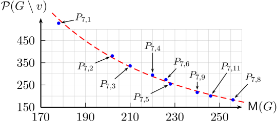
Figure 1: The periods and Martin invariants of primitive $\phi^{4}$ graphs [56] with $9$ vertices (7 loops decompleted). The dashed curve is a fit $\mathcal{P}(G\setminus v)\approx 32150\cdot\operatorname{\mathsf{M}}(G)^{-3.015}$.

Firstly, the Martin invariant and the period are correlated numerically. Graphs with smaller $\operatorname{\mathsf{M}}(G)$ tend to have larger periods. This approximate relation is illustrated in fig. 1 for the 4-regular graphs with $9$ vertices. As the plot shows, the period can be estimated surprisingly well from $\operatorname{\mathsf{M}}(G)$ and a simple power law. It is remarkable that the period integral (1.10) is so strongly correlated with the number of partitions into spanning trees (theorem 1.3). Furthermore, the period, and hence the Martin invariant, are also correlated to the Hepp bound [53], which is a tropical version of the period.

Secondly, even though the correlation just mentioned is only approximate, we find that the Martin sequence can detect precisely when two graphs have the same period. We calculated Martin invariants for a large number of 3- and 4-regular graphs (section 7). Comparing with the known periods [54, 7] and the Hepp bound, supports the following conjecture (we state a 3-regular version in 7.2).

Conjecture 1.10.

Cyclically 6-connected 4-regular graphs $G_{1}$ and $G_{2}$ have equal period $\mathcal{P}(G_{1}\setminus v_{1})=\mathcal{P}(G_{2}\setminus v_{2})$ if and only if they have equal Martin sequences $\operatorname{\mathsf{M}}(G_{1}^{\bullet})=\operatorname{\mathsf{M}}(G_{2}^{\bullet})$.

Via theorem 1.8, our conjecture implies that the $c_{2}$ invariants of graphs with equal periods agree at all primes. This is expected, also at prime powers, according to [57, Remark 2.11]. Our conjecture thus implies the case $q=p$ of [13, Conjecture 5].

1.10 also suggests that the period of a graph should be computable from the Martin sequence. Indeed, this can be achieved with Apéry limits, as will be discussed in forthcoming work. One important observation towards this is that Martin sequences are P-recursive (equivalently, their generating series are D-finite), as we prove in corollary 5.18.

There is another, in fact classical, connection between the Martin polynomial and quantum field theory: the Martin polynomial appears as the symmetry factor in $O(N)$ vector models. Only very recently, however, also the Martin invariant was noted to have a physical meaning in this context, namely it emerges at $N=-2$ for loop-erased random walks [66, 59]. We summarize this connection in section 2.1.

The sections of this paper are largely independent of each other.

1.4 Acknowledgments

Erik Panzer dedicates this work to his father, Michael Erhard Panzer, 1955–2022. In admiration, sorrow, gratitude, and loving memory.

We thank Simone Hu for discussions throughout this project and for confirming at an early stage that the available data for the $c_{2}$-invariant at prime $p=2$ is consistent with the relation to the Martin invariant. We further thank Simone for her work in refining the approach to the $c_{2}$-invariant via counting partitions of edges into trees and forests [41], which is also a key part of our work here. We also thank Francis Brown for suggesting the connection between $c_{2}$ and the diagonal coefficient, which allows for a simplification (lemma 6.16) of the proof of theorem 1.8 for primes $p\neq 3$.

Erik Panzer is funded as a Royal Society University Research Fellow through grant URF\R1\201473. He would like to thank the Isaac Newton Institute for Mathematical Sciences, Cambridge, for support and hospitality during the programme New connections in number theory and physics where work on this paper was undertaken. This event was supported by EPSRC grant no. EP/R014604/1. Karen Yeats is supported by an NSERC Discovery grant and the Canada Research Chairs program. Both authors are grateful for the hospitality of Perimeter Institute where part of this work was carried out. Research at Perimeter Institute is supported in part by the Government of Canada through the Department of Innovation, Science and Economic Development Canada and by the province of Ontario through the Ministry of Economic Development, Job Creation and Trade. This research was also supported in part by the Simons Foundation through the Simons Foundation Emmy Noether Fellows Program at Perimeter Institute.

Many figures in this paper were created using JaxoDraw [4].

2 The Martin polynomial

Let $G$ be an undirected graph where every vertex has even degree. Multiple edges between the same pair of vertices are allowed. At each vertex, we may also have any number of self-loops, that is, edges connecting the vertex to itself.

It will be helpful to think of graphs in terms of half-edges. The edges of the graph define a perfect matching of the half-edges of the graph, each half-edge is incident with exactly one vertex and a vertex $v$ has a corolla of incident half-edges. The set of the other halves of the edges incident to $v$ will be called the $h$-neighbourhood of $v$. The neighbourhood in the traditional graph theory sense, namely the set of vertices adjacent to $v$, can be recovered from the $h$-neighbourhood by replacing each half-edge in the $h$-neighbourhood with the vertex incident to that half-edge. When helpful for clarity we will call the graph theory notion of neighbourhood the $v$-neighbourhood.

Definition 2.1.

A transition at a vertex $v$ is a perfect matching of the half-edges of the $h$-neighbourhood of $v$. We write $\mathcal{T}_{G}(v)$ or simply $\mathcal{T}(v)$ for the set of all transitions at $v$. A transition system $P$ is a choice of one transition $P(v)\in\mathcal{T}(v)$ for every vertex of $G$.

Note that the notion of transition could equally well be defined as a matching of the corolla at $v$. The benefit of working with the $h$-neighbourhood is that for $v$ with no self-loops, and $\tau$ a transition at $v$, the graph $G_{\tau}$ (see the beginning of section 1) can be defined very naturally to be the graph obtained from $G$ by removing $v$ and its corolla and matching the half-edges of the $h$-neighbourhood of $v$ into new edges according to $\tau$.

Since the degree of every vertex $v$ is even, the sets $\mathcal{T}(v)$ are non-empty and transition systems exist. Concretely, a $v$ of degree $d$ has precisely

$$\left\lvert\mathcal{T}(v)\right\rvert=(d-1)!!=\frac{d!}{(d/2)!\cdot 2^{d/2}}$$ (2.1)

transitions, and the graph $G$ has $\prod_{v}(d_{v}-1)!!$ transition systems. A transition $\tau\in\mathcal{T}(v)$ can be interpreted as a traffic sign that forces anyone who enters $v$ from half-edge $e$, to leave by half-edge $e^{\prime}$ where $e^{\prime}$ is the partner of $e$ in the matching $\tau$. Traversed in this way, a transition system $P$ determines a partition of the edges of $G$ into circuits (closed trails). We write $|P|$ for the number of these circuits. For an example see fig. 2.

$P\in\left\{\vbox{\hbox{\includegraphics[scale={0.55}]{graphs/tran1}}},\quad\vbox{\hbox{\includegraphics[scale={0.55}]{graphs/tran2}}},\quad\vbox{\hbox{\includegraphics[scale={0.55}]{graphs/tran3}}}\right\}$   $\mathfrak{m}\left(\vbox{\hbox{\includegraphics[scale={0.6}]{graphs/2rosev}}},x\right)=1+(x-2)+1=x$

Figure 2: The three circuit partitions of a 2-rose and its Martin polynomial.

Definition 2.2.

The Martin polynomial is a sum over all transition systems, given by

$$\mathfrak{m}(G,x)=\sum_{P}(x-2)^{|P|-1}\in\mathbbm{Z}[x].$$ (2.2)

See table 1 for some examples. This polynomial was introduced by Martin [49] and extended by Las Vergnas [44]. In more recent literature, results for the Martin polynomial are often stated in terms of the circuit partition polynomial, defined as

$$J(G,x)=x\cdot\mathfrak{m}(G,x+2)=\sum_{P}x^{|P|}\in\mathbbm{Z}[x].$$ (2.3)

The coefficients of $J(G,x)=\sum_{k}r_{k}(G)x^{k}$ count the edge partitions into $k$ circuits. For example, the linear coefficient $r_{1}(G)=J^{\prime}(G,0)=\mathfrak{m}(G,2)$ counts the Eulerian circuits of $G$. The precise notion of circuit here is based on half-edges, see [6, p. 262] or [30] for details. Further evaluations of these polynomials can be found in [6, 29]. There is also an integral representation [51] for the values of $J(G,x)$ at positive integers $x$.

It is clear from definition 2.2 that $\mathfrak{m}(G,x)$ solves the recursion (1.1). Note however that if one applies a transition $\tau$ that pairs both ends of a self-loop, then $G_{\tau}$ will have a free loop, that is, a loop not connected to any vertex, which must still be counted. This can be avoided with

Lemma 2.3.

If $e$ is a self-loop at a vertex $v$ which has even degree $d\geq 2$, then

$$\mathfrak{m}(G,x)=(x+d-4)\cdot\mathfrak{m}(G\setminus e,x).$$ (2.4)

Proof.

Given any transition $\tau^{\prime}\in\mathcal{T}_{G^{\prime}}(v)$ of $G^{\prime}=G\setminus e$, we can pair the half-edges $e^{\prime},e^{\prime\prime}$ of $e$ to obtain a transition $\tau=\tau^{\prime}\cup\left\{e^{\prime},e^{\prime\prime}\right\}\in\mathcal{T}_{G}(v)$ in $G$. We can also pick one of the $d/2-1$ pairs $\left\{i,j\right\}\in\tau^{\prime}$ and interlace $e$ in either direction, to obtain two further transitions $\tau_{ij},\tau_{ji}\in\mathcal{T}_{G}(v)$ of the form $\tau_{ij}=\tau^{\prime}\setminus\left\{\left\{i,j\right\}\right\}\cup\left\{\left\{i,e^{\prime}\right\},\left\{j,e^{\prime\prime}\right\}\right\}$. These constructions produce every transition in $\mathcal{T}_{G}(v)$ exactly once.

We can thus group the sum (2.2) by transition systems of $P^{\prime}$ of $G^{\prime}$. For each $P^{\prime}$, we find one transition system $P$ of $G$ with $|P|=|P^{\prime}|+1$, and $d-2$ with $|P|=|P^{\prime}|$. Hence we conclude the claim, with the prefactor $(x-2)+(d-2)$. ∎

$G$
$\mathfrak{m}(G,x)$	$x$	$3x$	$x^{2}$	$x^{2}+6x$	$3x^{2}$	$5x^{2}+12x$	$15x^{2}+36x$

Table 1: Martin polynomials of some 4-regular graphs.

We can iterate lemma 2.3 to remove all self-loops [44, Proposition 4.1]. Hence we can compute $\mathfrak{m}(G,x)$ without ever creating free loops. As a special case, we find

$$\mathfrak{m}(C_{1}^{[k]},x)=x(x+2)\cdots(x+2k-4)$$ (2.5)

for the graph $C_{1}^{[k]}$ consisting of a single vertex with $k>1$ self-loops. This graph is called the $k$-rose. Induction via (1.1) with a rose as the base case shows that $\mathfrak{m}(G,x)$ is divisible by the right hand side of (2.5) whenever $G$ has a vertex of degree $2k$ or more.

Corollary 2.4.

If $G$ is $2k$-regular, has at least two vertices, and at least one self-loop, then $\mathfrak{m}(G,x)$ is divisible by $(x+2k-4)^{2}$.

Proof.

The self-loop $e$ gives one factor of $x+2k-4$ directly in (2.4). Since $G\setminus e$ still has at least one vertex of degree $2k$, we get a second factor from $\mathfrak{m}(G\setminus e,x)$. ∎

The Martin polynomial has numerous further interesting properties, however for our purposes we only use the above. Mainly, we conclude that the Martin invariant as defined in the introduction, definition 1.1, makes sense: the number $\operatorname{\mathsf{M}}(G)$ is uniquely determined, because we can obtain it from $\mathfrak{m}(G,x)$. Using this insight we give a new direct definition of the Martin invariant and then observe its equivalence with definition 1.1.

Definition 2.5.

The Martin invariant of a $2k$-regular graph is the derivative

$$\operatorname{\mathsf{M}}(G)=\frac{4\cdot(-1)^{k}}{(k-2)!\cdot(2k)!}\mathfrak{m}^{\prime}(G,4-2k)\in\mathbbm{Q}.$$ (2.6)

Since taking a derivative is a linear map, any derivative of $\mathfrak{m}$ inherits the recursion (1.1). Note also that $\mathfrak{m}^{\prime}(G,4-2k)$ vanishes for every $2k$-regular graph with a self-loop and more than one vertex, by corollary 2.4. Therefore, this derivative fulfils 1. and 3. of definition 1.1. Our choice of normalization (part 2. of definition 1.1) determines the prefactor in (2.6). Indeed, (2.6) gives

$$\operatorname{\mathsf{M}}(C_{1}^{[k]})=\frac{2^{k}}{(2k)!}\quad\text{and}\quad\operatorname{\mathsf{M}}(C_{2}^{[k]})=\frac{1}{k!}$$ (2.7)

for the rose and dipole graphs. The dipole $C_{2}^{[k]}=K_{2}^{[2k]}$ is a $2k$-fold edge, and its Martin invariant reduces to $(2k-1)!!$ times that of the rose by (1.1) and (2.1). For the rose itself, use (2.5). At three vertices, the only $2k$-regular graph without self-loops is the $k$-fold triangle, and expanding it at a vertex shows that, as claimed in part 2. of definition 1.1,

$$\operatorname{\mathsf{M}}(C_{3}^{[k]})=k!\cdot\operatorname{\mathsf{M}}(C_{2}^{[k]})=1.$$ (2.8)

Note that only $k!$ transitions produce a dipole; all other transitions produce self-loops and can hence be discarded for the computation of the Martin invariant.

Remark 2.6.

Our normalization (2.8) simplifies the 3-vertex cut product of proposition 3.10. This maximizes the analogy between $\operatorname{\mathsf{M}}$ and the Feynman period $\mathcal{P}$, because the latter also fulfils this product without extra factors [56, Theorem 2.1]. The downside is that we move outside of integers for the Martin invariants of $C_{1}^{[k]}$ and $C_{2}^{[k]}$ (though all graphs with at least 3 vertices have integer Martin invariant) and have an explicit factor $k!$ in the $2k$-edge cut product (1.3), which however has no direct analogue for Feynman periods, because graphs with such a cut have divergent Feynman integrals.

The Martin invariant was introduced for 4-regular graphs in [8]. In that paper, it is called $\beta_{4}$, and a different normalization is used. If $G$ has $n$ vertices, then

$$\operatorname{\mathsf{M}}(G)=\beta_{4}(G)\cdot 2^{n-3}.$$ (2.9)

The normalization of $\beta_{4}$ ensures that the totally decomposable graphs (see theorem 3.5) are precisely the graphs with $\beta_{4}(G)=1$, in analogy to how the series-parallel graphs are precisely the graphs with $\beta(G)=1$ for Crapo’s $\beta$ invariant [20, Proposition 8]. But in contrast to $\operatorname{\mathsf{M}}(G)$, for most graphs the number $\beta_{4}(G)$ is not an integer.

Apart from the paper [8], the only other result on the Martin invariant that we could find is [31, Theorem 4.6]. It states that for 4-regular graphs,

$$6\operatorname{\mathsf{M}}(G)=\mathfrak{m}^{\prime}(G,0)=\frac{J^{\prime}(G,-2)}{-2}=\sum_{C}r_{1}(G\setminus C)\cdot(-2)^{\kappa(C)-1}$$ (2.10)

is a sum over all subsets $C$ of edges such that every vertex of $G$ has degree 0 or 2 in $C$. In other words, $C$ is a vertex-disjoint union of cycles. We write $\kappa(C)$ for the number of these cycles, and $r_{1}(G)=\mathfrak{m}(G,2)=J^{\prime}(G,0)$ denotes the number of Eulerian circuits.

2.1 Vector model

In theoretical physics, the Martin polynomial appears as the symmetry factor $S_{G}$ in the $O(N)$ vector model. For details, see [42, Chapter 6]. In brief, this is the theory of $N$ real scalar fields $\phi=(\phi_{1},\ldots,\phi_{N})$ with Euclidean Lagrangian density

$$\mathscr{L}=\frac{1}{2}\sum_{i=1}^{N}\left(\left\lVert\nabla\phi_{i}\right\rVert^{2}+m^{2}\phi_{i}^{2}\right)+\frac{g}{4!}\left(\left\lVert\phi\right\rVert^{2}\right)^{2}.$$

The first term describes free scalars with equal mass $m$. The second term with the coupling constant $g$ encodes their interaction. This density is invariant under orthogonal transformations $\phi\mapsto T\phi$ with $T\in O(N)$. In terms of the symmetric tensor

$$\lambda_{ijkl}=\frac{1}{3}\left(\delta_{ij}\delta_{kl}+\delta_{ik}\delta_{jl}+\delta_{il}\delta_{jk}\right),$$ (2.11)

the quartic interaction can be written as

$$\left(\left\lVert\phi\right\rVert^{2}\right)^{2}=(\phi_{1}^{2}+\ldots+\phi_{N}^{2})^{2}=\sum_{i,j=1}^{N}\phi_{i}^{2}\phi_{j}^{2}=\sum_{i,j,k,l=1}^{N}\lambda_{ijkl}\phi_{i}\phi_{j}\phi_{k}\phi_{l}.$$

The perturbation theory of the $O(N)$ model thus differs from $\phi^{4}$ theory ($N=1$) only through a prefactor $S_{G}$ for each Feynman graph $G$. This factor counts all possible assignments of the field labels $\left\{1,\ldots,N\right\}$ to each edge compatibly with the expression for the interaction. Let $V$ and $E$ denote the sets of vertices and edges of $G$, and write $e_{v}^{1},\ldots,e_{v}^{4}$ for the four edges at a vertex. Then

$$S_{G}(N)=\sum_{c\colon E\rightarrow\left\{1,\ldots,N\right\}}\prod_{v\in V}\lambda_{c(e_{v}^{1}),c(e_{v}^{2}),c(e_{v}^{3}),c(e_{v}^{4})}$$ (2.12)

for every 4-regular (“vacuum”) graph $G$. Expanding each tensor in this product into the three terms in (2.11) corresponds to a sum over transition systems. The number of parts of the corresponding circuit partition gives the number of freely choosable field labels.

For a 4-regular graph with $n$ vertices, we can therefore identify

$$S_{G}(N)=3^{-n}\cdot J(G,N).$$ (2.13)

Corrections to the coupling constant are determined by graphs of the form $G\setminus v$, which have 4 free (“external”) half-edges. Their symmetry factor is [42, eq. (6.77)]

$$S_{G\setminus v}(N)=\frac{3S_{G}(N)}{N(N+2)}=\frac{\mathfrak{m}(G,N+2)}{3^{n-1}(N+2)}.$$

Since $\mathfrak{m}(G,x)$ is a multiple of $x$ by (2.5), it follows from (2.3) that $J(G,N)$ is a multiple of $N(N+2)$. Therefore, $S_{G\setminus v}(N)$ is a polynomial in $N$. One can therefore formally consider arbitrary values for $N$, even though the $O(N)$ vector model was defined above only for positive integers $N$. Upon setting $N=-2$, we obtain the Martin invariant:

$$S_{G\setminus v}(-2)=3^{1-n}\cdot\mathfrak{m}^{\prime}(G,0)=2\cdot 3^{2-n}\cdot\operatorname{\mathsf{M}}(G).$$ (2.14)

This was how we discovered the connection between the Martin invariant and Feynman symmetries: analyzing the symmetry factors for graphs with up to 13 vertices, we found that $N=-2$ is the only value for which identities like twist and duality hold.

Strikingly, the formal value $N=-2$ in the $O(N)$ vector model also describes a meaningful physical system. It was recently discovered [66, 59] that the formal “$O(-2)$” model describes loop erased random walks (LERW). The value $N=-2$ is therefore distinguished not only by the additional mathematical properties of the Martin invariant (the full Martin polynomial does not fulfil identities like twist or duality), but it also corresponds to an exceptional field theory.

3 Connectivity

We say that a graph $G$ is $d$-regular if every vertex of $G$ has degree $d$. Except for proposition 3.8, we always assume that the degree is even, and hence denote it as $2k$.

$G=\quad\vbox{\hbox{\includegraphics[scale={0.8}]{graphs/splitoff}}}$   $\mapsto$  $G^{\prime}=\quad\vbox{\hbox{\includegraphics[scale={0.8}]{graphs/splitoff2}}}$

Figure 3: Splitting off a pair $(va,vb)$ of edges.

Lemma 3.1.

If $G$ is $2k$-regular but not $2k$-edge connected, then $\operatorname{\mathsf{M}}(G)=0$.

Proof.

Consider a minimal edge cut $C$ of $G$, with size $\left\lvert C\right\rvert=2s<2k$. Let $G_{1}$ and $G_{2}$ denote the two sides of the cut, so that $G\setminus C=G_{1}\sqcup G_{2}$. If $G_{1}$ consists of only one vertex, then this vertex has $k-s>0$ self-loops, and therefore $\operatorname{\mathsf{M}}(G)=0$. Otherwise, if $G_{1}$ has several vertices, pick one and call it $v$. For every transition $\tau$ at $v$, the edges of $C$ in $G_{\tau}$ define a (not necessarily minimal) edge-cut of $G_{\tau}$, hence $G_{\tau}$ is at most $2s$-edge connected. By induction over the total number of vertices, we may assume that $\operatorname{\mathsf{M}}(G_{\tau})=0$, and therefore conclude the induction step that $\operatorname{\mathsf{M}}(G)=0$ as well, by (1.1). ∎

Theorem 3.2.

If $G$ is $2k$-regular and $2k$-edge connected, and $v$ denotes any vertex, then there exists a transition $\tau\in\mathcal{T}(v)$ such that $G_{\tau}$ is $2k$-edge connected.

Proof.

Let $\lambda_{G}(x,y)$ denote the maximal number of edge-disjoint walks in $G$, with endpoints at vertices $x\neq y$. By Menger’s theorem, the $2k$-edge connectedness of $G$ implies that $\lambda_{G}(x,y)\geq 2k$ for all pairs $x\neq y$. In fact, since $G$ is $2k$-regular, equality holds. Lovász’ vertex splitting-off lemma [47, Theorem 1] shows that at any vertex $v$ in any Eulerian graph $G$, one can find two different edges $va$ and $vb$, such that the graph $G^{\prime}=G-va-vb+ab$ (see fig. 3) has the following property: for every pair $x\neq y$ of vertices different from $v$, one has

$$\lambda_{G}(x,y)=\lambda_{G^{\prime}}(x,y).$$

Iterating this lemma $k$ times produces a transition $\tau$ with $\lambda_{G_{\tau}}(x,y)=\lambda_{G}(x,y)=2k$, therefore $G_{\tau}$ is $2k$-edge connected. ∎

Corollary 3.3.

If $G$ is $2k$-regular and $2k$-edge connected, then $\operatorname{\mathsf{M}}(G)>0$.

Proof.

By (1.1), we have $\operatorname{\mathsf{M}}(G)\geq\operatorname{\mathsf{M}}(G_{\tau})$ for any transition of $G$. Choosing $\tau$ as in theorem 3.2, we can ensure that $G_{\tau}$ is $2k$-edge connected. Hence, by induction, it suffices to study the case where $G$ has only $3$ vertices. Since $2k$-edge connectedness implies the absence of self-loops, $\operatorname{\mathsf{M}}(G)=1>0$ by definition 1.1. ∎

Together with lemma 3.1, corollary 3.3 proves that for a graph $G$ that is $2k$-regular, $\operatorname{\mathsf{M}}(G)>0$ if and only if $G$ is $2k$-edge connected. This settles parts 1 and 2 of theorem 1.2. We now show part 3:

Lemma 3.4.

Let $G$ be $2k$-regular and $C$ a $2k$-edge cut of $G$. Let $G_{1}^{\prime}\sqcup G_{2}^{\prime}=G\setminus C$ denote the two sides of the cut, and write $G_{i}$ for the graph obtained from $G_{i}$ by adding a vertex connected to the ends of $C$ in $G_{i}$, see (1.3). Then $\operatorname{\mathsf{M}}(G)=k!\cdot\operatorname{\mathsf{M}}(G_{1})\cdot\operatorname{\mathsf{M}}(G_{2})$.

Proof.

We proceed by induction over the number of vertices of $G_{2}^{\prime}$. If $G_{2}^{\prime}$ has only one vertex, then $G_{2}$ is a $2k$-fold edge and $G_{1}=G$. The claim is thus trivial, $\operatorname{\mathsf{M}}(G)=\operatorname{\mathsf{M}}(G)$, because $\operatorname{\mathsf{M}}(G_{2})=\operatorname{\mathsf{M}}(K_{2}^{[2k]})=1/(k!)$. If $G_{2}^{\prime}$ has more than one vertex, pick any vertex $v$ in $G_{2}^{\prime}$. Using the induction hypothesis, expanding at $v$ yields

$$\operatorname{\mathsf{M}}(G)=\sum_{\tau\in\mathcal{T}(v)}\operatorname{\mathsf{M}}(G_{\tau})=k!\sum_{\tau\in\mathcal{T}(v)}\operatorname{\mathsf{M}}((G_{\tau})_{1})\cdot\operatorname{\mathsf{M}}((G_{\tau})_{2}),$$

because the edges of $C$ define a $2k$-edge cut in every $G_{\tau}$. If $\tau$ pairs any edges in $C$ with each other, then $C$ induces in $G_{\tau}$ an edge-cut of size less than $2k$, hence such transitions can be dropped from the sum by lemma 3.1. The remaining transitions commute with the cut: the side $(G_{\tau})_{1}=G_{1}$ is the same for all $\tau$, and $(G_{\tau})_{2}=(G_{2})_{\tau}$. Hence the right-hand side sums to the claim. Note that the dropped $\tau$ are precisely those that produce a self-loop in $(G_{2})_{\tau}$ at the extra vertex, hence their absence causes no error to $\operatorname{\mathsf{M}}(G_{2})$. ∎

3.1 Decompositions and lower bounds

We saw above that $\operatorname{\mathsf{M}}(G)>0$ if $G$ is $2k$-regular and $2k$-edge connected. In this subsection, we give a combinatorial description of all such graphs which, at a given number of vertices, minimize the Martin invariant. This is closely related to factorizations with respect to the $2k$-edge cut product from lemma 3.4, for which we prove uniqueness (proposition 3.8).

By repeated replacements $G\mapsto G_{1},G_{2}$ along $2k$-edge cuts, we can decompose every $2k$-edge connected $2k$-regular graph with $\geq 3$ vertices into a sequence of graphs $G_{1},\ldots,G_{p}$ until each graph in the sequence is cyclically $(2k+2)$-connected and has at least 3 vertices. Following [8, 35], we call such a sequence a decomposition of $G$. Iterating (1.1), note that

$$\operatorname{\mathsf{M}}(G)=(k!)^{p-1}\cdot\operatorname{\mathsf{M}}(G_{1})\cdots\operatorname{\mathsf{M}}(G_{p}).$$ (3.1)

We call $G$ totally decomposable [8] if it has a decomposition such that all $G_{i}$ have only 3 vertices, see fig. 4. By (3.1), such a graph, with $n$ vertices, has $\operatorname{\mathsf{M}}(G)=(k!)^{n-3}$. By induction one sees easily that any totally decomposable graph has at least two edges with multiplicity $k$. Decomposing by cutting off such an edge at each step we end with the $k$-fold triangle. Therefore, reversing this we get that totally decomposable graphs can be constructed from the $k$-fold triangle by repeatedly replacing a vertex with a $k$-fold edge.

$\vbox{\hbox{\includegraphics[scale={0.5}]{graphs/C52cut}}}\quad\mapsto\quad\vbox{\hbox{\includegraphics[scale={0.5}]{graphs/C42cut}}},\vbox{\hbox{\includegraphics[scale={0.4}]{graphs/C32}}}\quad\mapsto\quad\vbox{\hbox{\includegraphics[scale={0.4}]{graphs/C32}}},\vbox{\hbox{\includegraphics[scale={0.4}]{graphs/C32}}},\vbox{\hbox{\includegraphics[scale={0.4}]{graphs/C32}}}\quad\reflectbox{$\mapsto$}\quad\vbox{\hbox{\includegraphics[scale={0.4}]{graphs/C32}}},\vbox{\hbox{\includegraphics[scale={0.5}]{graphs/v4totcut}}}\quad\reflectbox{$\mapsto$}\quad\vbox{\hbox{\includegraphics[scale={0.5}]{graphs/v5totcut}}}$

Figure 4: Decomposition of two totally decomposable graphs into 3 copies of $C_{3}^{[2]}$.

For example, cutting off $m\geq 2$ consecutive vertices from a $k$-fold cycle,

$$C_{n}^{[k]}\mapsto C_{m+1}^{[k]},C_{n-m+1}^{[k]}$$

terminates in a decomposition of $C_{n}^{[k]}$ into $n-2$ copies of the $k$-fold triangle $C_{3}^{[k]}=K_{3}^{[k]}$.

The totally decomposable graphs minimize the Martin invariant:

Theorem 3.5.

A $2k$-regular, $2k$-edge connected graph $G$ with $n\geq 2$ vertices has $M(G)\geq(k!)^{n-3}$, and equality holds if and only if $G$ is totally decomposable.

The 4-regular case of this result was known previously [8, Corollary 5.6]. To prove theorem 3.5, we first establish the lower bound, which strengthens corollary 3.3:

Proposition 3.6.

Suppose that the graph $G$ is $2k$-regular, $2k$-edge connected, and that it has $n\geq 2$ vertices. Then $\operatorname{\mathsf{M}}(G)\geq(k!)^{n-3}$.

Proof.

As in the proof of theorem 3.2, let $\lambda_{G}(x,y)$ denote the maximum number of edge-disjoint paths between vertices $x$ and $y\neq x$. Given $G$ and fixing a vertex $v$, we call a pair $(va,vb)$ of edges at $v$ admissible if $\lambda_{G^{\prime}}(x,y)\geq 2k$ for all $x\neq y$ with $x,y\neq v$, in the graph $G^{\prime}=G-va-vb+ab$.

It was shown in [2, Theorem 2.12] that if $v$ has even degree $d$ and $\lambda_{G}(x,y)\geq 2k$ for all $x\neq y$ different from $v$, then for any edge $va$, there are at least $d/2$ other edges $vb$ such that the pair $(va,vb)$ is admissible. Applying this argument to $G^{\prime}$, where $v$ has degree $2k-2$, and iterating, we conclude that there are at least

$$\frac{2k}{2}\cdot\frac{2k-2}{2}\cdots\frac{2}{2}=k!$$

transitions $\tau\in\mathcal{T}(G)$ such that $G_{\tau}$ is $2k$-edge connected. So if $c_{n}$ denotes the minimum value of $\operatorname{\mathsf{M}}(G)$ over all $2k$-regular, $2k$-edge connected graphs $G$ with $n$ vertices, then taking only those transitions into account, the sum (1.1) shows that

$$c_{n}\geq k!\cdot c_{n-1}.$$

We conclude that $c_{n}\geq(k!)^{n-3}$ by induction over $n$ and $c_{3}=1$. ∎

To finish the proof of theorem 3.5, recall that $\operatorname{\mathsf{M}}(G)=(k!)^{n-3}$ if $G$ is totally decomposable. If $G$ is not totally decomposable, then any decomposition $G_{1},\ldots,G_{p}$ has at least one factor with at least $4$ vertices. Let $G_{1}$ be such a factor, and let $n_{i}$ denote the number of vertices in $G_{i}$. Then by (3.1) and proposition 3.6,

$$\operatorname{\mathsf{M}}(G)\geq(k!)^{p-1}\cdot\operatorname{\mathsf{M}}(G_{1})\cdot(k!)^{n_{2}-3}\cdots(k!)^{n_{p}-3}=(k!)^{n-3}\cdot\frac{\operatorname{\mathsf{M}}(G_{1})}{(k!)^{n_{1}-3}}$$

because $n_{1}+\ldots+n_{p}=n+2(p-1)$. Therefore, $\operatorname{\mathsf{M}}(G)>(k!)^{n-3}$ follows from our next lemma.

Lemma 3.7.

If $G$ is $2k$-regular and cyclically $2k+2$ connected, with $n\geq 4$ vertices, then $\operatorname{\mathsf{M}}(G)>(k!)^{n-3}$.

Proof.

Pick any vertex $v$ in $G$. Consider two edges $va$, $vb$ at $v$ with different endpoints $a\neq b$. We first show that such a pair $(va,vb)$ is admissible:

Suppose that $(va,vb)$ is not admissible. Then $G^{\prime}=G-va-vb+ab$ has an edge cut $C^{\prime}$ of size $\left\lvert C^{\prime}\right\rvert<2k$, with at least one vertex $x\neq v$ and at least one vertex $y\neq v$ on each side of $C^{\prime}$. Let $V(G)=X\sqcup Y$ denote the vertex bipartition corresponding to $C^{\prime}$, with $v,x\in X$ and $y\in Y$. We show that the cut $C$ of $G$ with this bipartition contradicts the cyclic $2k+2$ connectivity of $G$:

• If $a,b\in X$, then $C=C^{\prime}$ has size $\left\lvert C\right\rvert=\left\lvert C^{\prime}\right\rvert<2k$.

• If $a\in X$ and $b\in Y$, then $ab\in C^{\prime}$ and $C=C^{\prime}-ab+vb$ has size $\left\lvert C\right\rvert=\left\lvert C^{\prime}\right\rvert<2k$.

• If $a,b\in Y$ (see fig. 5), then $C=C^{\prime}+va+vb$ has size $\left\lvert C\right\rvert=\left\lvert C^{\prime}\right\rvert+2\leq 2k+1$. Since all vertices have even degree, $\left\lvert C\right\rvert$ must be even, thus $\left\lvert C\right\rvert\leq 2k$. Note that neither side of $C$ is a single vertex: $\left\lvert X\right\rvert\geq\left\lvert\left\{v,x\right\}\right\rvert=2$ and $\left\lvert Y\right\rvert\geq\left\lvert\left\{a,b\right\}\right\rvert=2$.

The third point directly contradicts cyclic $2k+2$ connectivity while the first two either contradict $2k$ regularity if one side of the cut is a single vertex and cyclic $2k+2$ connectivity otherwise.

$G=\vbox{\hbox{\includegraphics[scale={0.9}]{graphs/XYab}}}$   $G^{\prime}=\vbox{\hbox{\includegraphics[scale={0.9}]{graphs/XYabp}}}$

Figure 5: Illustration for the proof of lemma 3.7: A non-admissible pair $(va,vb)$ implies the existence of a forbidden cut $C$ in $G$.

Now pick any neighbour $a$ of $v$. The number $s$ of edges between $a$ and $v$ is at most $k-1$, as otherwise, the subgraph induced by $a$ and $v$ would constitute a cut of size $2\cdot 2k-2s\leq 2k$ with at least 2 vertices on each side since $G$ has $n\geq 4$ vertices. Therefore, at least $2k-(k-1)=k+1$ edges at $v$ have endpoints $b\neq a$. Since such pairs $(va,vb)$ are admissible as we showed above, we find at least $k+1$ admissible pairs containing $va$. After splitting off such a pair, we invoke [2, Theorem 2.12] repeatedly, as in the proof of proposition 3.6, to conclude that there are at least

$$(k+1)\cdot(k-1)!$$

transitions $\tau\in\mathcal{T}(v)$ such that $G_{\tau}$ is $2k$-edge connected. Considering only those summands and using (1.1), we learn that $\operatorname{\mathsf{M}}(G)\geq(k+1)\cdot(k-1)!\cdot(k!)^{n-4}>(k!)^{n-3}$. ∎

According to our definition earlier, a decomposition of a $d=2k$-regular graph is obtained after a maximal sequence of $d$-edge cuts. Such a sequence of cuts is rarely unique. For example, to decompose a k-fold cycle on 6 vertices, we can choose to cut off either 2 or 3 vertices in the first step, which leads to two different sequences of cuts:

• $C_{6}^{[k]}\mapsto C_{5}^{[k]}C_{3}^{[k]}\mapsto C_{4}^{[k]}C_{3}^{[k]}C_{3}^{[k]}\mapsto C_{3}^{[k]}C_{3}^{[k]}C_{3}^{[k]}C_{3}^{[k]}$

• $C_{6}^{[k]}\mapsto C_{4}^{[k]}C_{4}^{[k]}\mapsto C_{4}^{[k]}C_{3}^{[k]}C_{3}^{[k]}\mapsto C_{3}^{[k]}C_{3}^{[k]}C_{3}^{[k]}C_{3}^{[k]}$

However, note that the resulting decomposition is the same: we obtain four times the $k$-fold triangle, even though we constructed those triangles by different sequences of cuts.

We close this section by showing that decompositions $G\mapsto G_{1}\cdots G_{p}$ are always unique. Here, unique is meant in the sense of multisets (lists up to reordering) of isomorphism classes of graphs. Our proof works for arbitrary degrees. For the cubic case $d=3$, a proof of uniqueness was given in [35, Theorem 3.5].

Proposition 3.8.

Decompositions of $d$-edge connected graphs are unique.

Proof.

Let two decompositions $A=A_{1}\cdots A_{p}$ and $B=B_{1}\cdots B_{q}$ of $G$ be given. We call an edge cut trivial if one side of it consists of a single vertex. If $G$ has does not have any non-trivial $d$-edge cut, then we must have $p=q=1$ and $A_{1}=B_{1}=G$ is indeed unique.

If $G$ does have a non-trivial $d$-edge cut, then $G$ is not cyclically $d+1$ connected, hence we must have $p,q\geq 2$. Let $C$ and $D$ denote the $d$-edge cuts used in the first step of a construction of the decompositions $A$ and $B$, respectively, such that

$$A=A^{\prime}A^{\prime\prime}\qquad\text{and}\qquad B=B^{\prime}B^{\prime\prime}$$

where $A^{\prime}$ and $A^{\prime\prime}$ are decompositions of the two sides of $C$, and similarly $B^{\prime},B^{\prime\prime}$ for $D$. By induction over the size of $G$, we may use that $A^{\prime},A^{\prime\prime},B^{\prime},B^{\prime\prime}$ are unique.

The two cuts determine a partition of $G\setminus(C\cup D)=G_{1}\sqcup G_{2}\sqcup G_{3}\sqcup G_{4}$ into four subgraphs, such that $C=[G_{1}\cup G_{4},G_{2}\cup G_{3}]$ and $D=[G_{1}\cup G_{2},G_{3}\cup G_{4}]$, where $[X,Y]$ denotes all edges of $G$ with one end in $X$ and the other end in $Y$. Let $n_{ij}=\left\lvert[G_{i},G_{j}]\right\rvert$ denote the number of edges in $G$ between $G_{i}$ and $G_{j}$. Note that

$$n_{12}+n_{13}+n_{24}+n_{34}=\left\lvert C\right\rvert=d\quad\text{and}\quad n_{13}+n_{14}+n_{23}+n_{24}=\left\lvert D\right\rvert=d. \sharp$$ ()

If two of the subgraphs $G_{i}$ are empty, we have $C=D$ and therefore $A^{\prime}=B^{\prime}$ and $A^{\prime\prime}=B^{\prime\prime}$ by induction, hence $A=B$.

$G$	$G_{12}^{\prime}$	$G_{3}^{\prime}$	$G_{23}^{\prime}$	$G_{1}^{\prime}$	$G_{2}^{\prime}$

Figure 6: Graphs that arise in the decomposition for two cuts $C$ and $D$ with $G_{4}=\emptyset$.

If only one of the subgraphs is empty, say $G_{4}=\emptyset$, then $A^{\prime}$ and $A^{\prime\prime}$ are by definition decompositions of the graphs $G_{1}^{\prime}$ and $G_{23}^{\prime}$ obtained from $G_{1}$ and $G_{2}\cup G_{3}\cup[G_{2},G_{3}]$, respectively, by reconnecting the edges $C$ to an extra vertex. Similarly, $B^{\prime}$ and $B^{\prime\prime}$ are decompositions of the graphs $G_{3}^{\prime},G_{12}^{\prime}$ obtained from $G_{3}$ and $G_{1}\cup G_{2}\cup[G_{1},G_{2}]$, see fig. 6. Note that $C$ defines a cut $G_{12}^{\prime}\mapsto G_{1}^{\prime}G_{2}^{\prime}$ and $D$ defines a cut $G_{23}^{\prime}\mapsto G_{3}^{\prime}G_{2}^{\prime}$, such that

$$A^{\prime\prime}=OB^{\prime}\qquad\text{and}\qquad B^{\prime\prime}=OA^{\prime}$$

in terms of a decomposition $O$ of the graph $G_{2}^{\prime}$ obtained from $G$ by replacing $G_{1}$ and $G_{3}$ by single vertices. Here we exploited the uniqueness of $A^{\prime\prime}$ and $B^{\prime\prime}$ (induction hypothesis), which allows us to compute them using any cut we like. We conclude that $A^{\prime}A^{\prime\prime}=A^{\prime}OB^{\prime}=B^{\prime}B^{\prime\prime}$, up to order.

Finally, consider the case when all four subgraphs $G_{i}$ are non-empty. Since $G$ is $d$-edge connected, we have the lower bounds

$$n_{12}+n_{13}+n_{14} \geq d, n_{12}+n_{23}+n_{24} \geq d,$$

$$n_{13}+n_{23}+n_{34} \geq d, n_{14}+n_{24}+n_{34} \geq d.$$

Combined with ($\sharp$ ‣ 3.1), this system has a unique solution, given by $n_{13}=n_{24}=0$ and $n_{12}=n_{14}=n_{23}=n_{34}=d/2$. Therefore, $d$ must be even, and the edges $[G_{1},G_{2}\cup G_{4}]$ constitute a cut of size $n_{12}+n_{14}=d$ that separates $G_{1}$ from the rest of $G$. Analogously, the other $G_{i}$ each can be cut out along $d$ edges. Let $G\mapsto G_{14}^{\prime}G_{23}^{\prime}$ denote the graphs created by the cut $C$, so that $A^{\prime}$ and $A^{\prime\prime}$ are decompositions of $G_{14}^{\prime}$ and $G_{23}^{\prime}$, respectively. Here, $G_{ij}$ is obtained from $G_{i}\cup G_{j}\cup[G_{i},G_{j}]$ by joining the cut edges to a new vertex (see fig. 7). Using the cuts $[G_{2},G_{1}\cup G_{3}]$ and $[G_{3},G_{1}\cup G_{4}]$ of $G_{23}^{\prime}$, we can decompose

$G$	$G_{23}^{\prime}$	$G_{14}^{\prime}$	$G_{1}^{\prime}$	$G_{2}^{\prime}$	$G_{3}^{\prime}$	$G_{4}^{\prime}$

Figure 7: Graphs that arise in the decomposition of two cuts $C,D$ with all $G_{i}\neq\emptyset$.

$$G_{23}^{\prime}\mapsto G_{2}^{\prime}G_{3}^{\prime}C_{3}^{[d/2]}\quad\text{and thus find}\quad A^{\prime}=O_{2}O_{3}C_{3}^{[d/2]}$$

where $O_{i}$ denotes a decomposition of the graph $G_{i}^{\prime}$ obtained from $G_{i}$ (see fig. 7). Again, we use here inductively that the decomposition of $G_{23}^{\prime}$ is unique. In the same manner, we find $A^{\prime\prime}=O_{1}O_{4}C_{3}^{[d/2]}$ and therefore

$$A^{\prime}A^{\prime\prime}=O_{1}O_{2}O_{3}O_{4}C_{3}^{[d/2]}C_{3}^{[d/2]}.$$

Clearly, applying the same procedure to $D$, i.e. decomposing $G\mapsto G_{12}^{\prime}G_{34}^{\prime}$ and then $G_{12}^{\prime}\mapsto G_{1}^{\prime}G_{2}^{\prime}C_{3}^{[d/2]}$ and $G_{34}^{\prime}\mapsto G_{3}^{\prime}G_{4}^{\prime}C_{3}^{[d/2]}$ we obtain the same result for $B^{\prime}B^{\prime\prime}$. ∎

3.2 Product and twist

For the product identity (1.4), consider a $3$-vertex cut $S=\left\{v_{1},v_{2},v_{3}\right\}$ of a $2k$-regular graph $G$. More precisely, fix a bipartition $E=E_{1}\sqcup E_{2}$ of the edges of $G$ such that the only vertices shared by $E_{1}$ and $E_{2}$ are in $S$. Let $d_{i}$ denote the number of edges at $v_{i}$ that belong to $E_{1}$, then the other $2k-d_{i}$ edges at $v_{i}$ belong to $E_{2}$. Set

$$n_{12}=\frac{d_{1}+d_{2}-d_{3}}{2},\quad n_{13}=\frac{d_{1}+d_{3}-d_{2}}{2},\quad n_{23}=\frac{d_{2}+d_{3}-d_{1}}{2}.$$ (3.2)

These are integers, because $d_{1}+d_{2}+d_{3}$ is the size of an edge cut and hence even. Note that in any graph where every vertex has even degree, all edge cuts are even.

Lemma 3.9.

If $G$ is $2k$-edge connected, then $n_{12},n_{13},n_{23}\geq 0$.

Proof.

Suppose that $n_{12}<0$. Then $d_{1}+d_{2}<d_{3}$, hence $d_{1}+d_{2}+(2k-d_{3})<2k$. So the edges at $v_{1},v_{2}$ in $E_{1}$ together with the edges at $v_{3}$ in $E_{2}$ form a cut of $G$ with size less than $2k$, contradicting the assumption on $G$. ∎

Now we state and prove the product identity for the Martin invariant introduced in (1.4).

Proposition 3.10.

Let $G$ be $2k$-regular and $2k$-edge connected, with a 3-vertex cut. Then the two sides of the cut can be turned into $2k$-regular graphs $G_{1}$ and $G_{2}$, by adding edges (but no self-loops) between the cut vertices. Furthermore, we have

$$\operatorname{\mathsf{M}}(G)=\operatorname{\mathsf{M}}(G_{1})\cdot\operatorname{\mathsf{M}}(G_{2}).$$

Proof.

With notation as above, lemma 3.9 implies that we can construct a $2k$-regular graph $G_{2}$ from $E_{2}$ by adding $n_{ij}$ edges connecting $v_{i}$ and $v_{j}$, for each of the three pairs $ij=12,13,23$. By a symmetric construction we get $G_{1}$ from $E_{1}$. This proves the first claim of proposition 3.10. In fact, (3.2) is the unique solution to the constraints $n_{ij}+n_{ik}+d_{i}=2k$, so this is the only way to add non-self loop edges to $E_{2}$ that leaves a $2k$-regular graph.

To complete the proof of proposition 3.10, we exploit that the identity (1.4) is linear in each factor. More precisely, for any vertex $v\notin S$ that belongs to $G_{1}$, we can apply transitions $\tau\in\mathcal{T}(v)$ at $v$ on both sides: in $G$ and in $G_{1}$. Since $\tau$ only glues edges from $E_{1}$, it leaves $G_{2}$ unchanged and the cut $S$ remains a cut of $G_{\tau}$, such that $(G_{1})_{\tau}=(G_{\tau})_{1}$ and $(G_{\tau})_{2}=G_{2}$. The expansion (1.1) at $v$ therefore reduces the claim to the statement that $\operatorname{\mathsf{M}}(G_{\tau})=\operatorname{\mathsf{M}}((G_{\tau})_{1})\operatorname{\mathsf{M}}((G_{\tau})_{2})$. An induction over the number of vertices therefore reduces the claim to trivial base cases:

• If $G$ has a self-loop, then this self-loop is also a self-loop in $G_{1}$ or $G_{2}$, so the identity holds trivially because both sides are zero.

• When only 3 vertices are left, namely the vertices $S$, and $G$ has no self-loops, then all 3 graphs $G$, $G_{1}$, and $G_{2}$, are necessarily identical to the $k$-fold triangle. The identity then holds due to our normalization $\operatorname{\mathsf{M}}(C_{3}^{[k]})=1$.

∎

With the same induction principle, we now prove the twist identity (1.5). Suppose we are given a graph $G$ with a $4$-vertex cut $S=\left\{v_{1},v_{2},v_{3},v_{4}\right\}$ and a bipartition $E=E_{1}\sqcup E_{2}$ of the edges, such that all vertices shared between $E_{1}$ and $E_{2}$ are contained in $S$. Let $d_{i}$ denote the number of edges at $v_{i}$ that belong to $E_{1}$. Schnetz introduced the twist operation [56, §2.6], which is illustrated in (1.5).

Definition 3.11.

If $d_{1}=d_{2}$ and $d_{3}=d_{4}$, then the twist of $G$ is the graph $G^{\prime}$ obtained from $G$ by replacing every edge $e\in E_{1}$ with an endpoint in $S$, $e=uv_{i}$, by $uv_{\sigma(i)}$, where $\sigma=(1\ 2)(3\ 4)$ is the double transposition that swaps $v_{1}\leftrightarrow v_{2}$ and $v_{3}\leftrightarrow v_{4}$.

At a 4-vertex cut with $d_{1}=d_{2}=d_{3}=d_{4}$, one can construct 3 twists, by relabeling $v_{i}$ or, equivalently, using the other double transpositions $\sigma=(1\ 3)(2\ 4)$ and $\sigma=(1\ 4)(2\ 3)$. If we fix $S$ and $\sigma$, then the twist is an involution: $G$ is the twist of $G^{\prime}$. Now we state and prove the twist identity for the Martin invariant introduced in (1.5).

Proposition 3.12.

If two regular graphs of even degree are obtained from each other by a double transposition on one side of a 4-vertex cut, then their Martin invariants agree:

$$\operatorname{\mathsf{M}}\Bigg{(}\ \vbox{\hbox{\includegraphics[scale={0.3}]{graphs/4cut}}}\ \Bigg{)}=\operatorname{\mathsf{M}}\Bigg{(}\ \vbox{\hbox{\includegraphics[scale={0.3}]{graphs/twist}}}\ \Bigg{)}.$$

Proof.

Let $G,S,E,d_{i}$ be as above. As in the proof of proposition 3.10 we can use the expansion (1.1) into transitions at any vertex $v\notin S$, to reduce the twist identity

$$\operatorname{\mathsf{M}}(G)=\operatorname{\mathsf{M}}(G^{\prime})$$

to the case where $G$ has no vertices other than $S$. If $G$ contains a self-loop, so does $G^{\prime}$, and the identity becomes trivial since both sides are zero. Hence we may assume that there are no self-loops in $G$. In this situation, $E_{1}$ is completely determined by the numbers $n_{ij}$ of edges in $E_{1}$ that connect $v_{i}$ with $v_{j}$. Due to the constraints

$$n_{12}+n_{13}+n_{14} =d_{1}=d_{2}=n_{12}+n_{23}+n_{24}\quad\text{and}$$

$$n_{13}+n_{23}+n_{34} =d_{3}=d_{4}=n_{14}+n_{24}+n_{34},$$

we must have $n_{13}=n_{24}$ and $n_{14}=n_{23}$. This shows that $G=G^{\prime}$, because the twist changes $E_{1}$ into $E_{1}^{\prime}$ with $n_{ij}^{\prime}=n_{\sigma(i)\sigma(j)}$. The base case of our induction for the proof of the twist identity is therefore trivial. ∎

4 Permanent

As our first case of a previously studied graph invariant with the same symmetries as the period and which can now be explained in terms of the Martin invariant, we will study a permanent-based invariant due to Iain Crump [23, 22].

Let $G$ be a $2k$-regular graph with $n+2$ vertices. Then $G$ has $kn+2k$ edges. Pick two different vertices, called $\infty$ and $0$, and orient each edge. We assume that there are no self-loops at $\infty$. Then the directed graph $G\setminus\infty$ has $n+1$ vertices and $kn$ edges. Its reduced incidence matrix is the $n\times kn$ matrix

$$A_{ve}=\begin{cases}+1&\text{if $e$ points to $v$},\\ -1&\text{if $e$ comes from $v$},\\ \phantom{-}0&\text{if $e$ is not incident to $v$,}\end{cases}$$ (4.1)

whose rows are indexed by the vertices $v\neq 0,\infty$ and whose columns are indexed by the edges $e$ of $G$ that are not attached to $\infty$. Stacking $k$ copies of $A$ produces a $kn\times kn$ square matrix, denoted $A^{[k]}$. Its permanent defines an integer

$$\operatorname{Perm}(G)\mathrel{\mathop{:}}=\operatorname{perm}A^{[k]}=\operatorname{perm}\begin{pmatrix}A\\ \vdots\\ A\\ \end{pmatrix}.$$ (4.2)

This number $\operatorname{Perm}(G)$ depends on the choice of $0$, $\infty$, and the orientation of the edges used to write down $A$. However, it was shown in [23] that the residue

$$\operatorname{Perm}(G)\mod(k+1)$$

depends on all these choices only up to a sign. Equivalently, the residue of $\operatorname{Perm}(G)^{2}$ is a well-defined invariant of the graph $G$. This invariant respects the known identities of Feynman periods [23], see also remark 4.3. Moreover, the sequence $\operatorname{Perm}(G^{[r]})^{2}\mod(kr+1)$ of permanents of all duplicated graphs is a very strong invariant of $G$ in that it distinguishes almost all Feynman periods [21, 22].

In this section, we show that the permanent is determined by the Martin invariant. Note that the repetition of rows makes $\operatorname{Perm}(G)$ a multiple of $(k!)^{n}$. It is therefore congruent to zero, unless the modulus $k+1$ is prime [23, Proposition 13].

Theorem 4.1.

For every $2k$-regular graph $G$ with $n\geq 3$ vertices such that $p=k+1\geq 3$ is prime, we have

$$\operatorname{\mathsf{M}}(G)\equiv(-1)^{n-1}\operatorname{Perm}(G)^{2}\mod p.$$ (4.3)

Note that each term of the sequence $\operatorname{Perm}(G^{[r]})^{2}\mod(kr+1)$ for which $kr+1$ is prime immediately also falls under this theorem and so is determined by the Martin invariant on the $G^{[r]}$.

$G=\vbox{\hbox{\includegraphics[scale={0.5}]{graphs/octa}}}$   $A=\begin{pmatrix}\phantom{-}1&\phantom{-}0&\phantom{-}0&-1&\ 1&\ 0&\ 0&\ 0\\ -1&\phantom{-}1&\phantom{-}0&\phantom{-}0&\ 0&\ 1&\ 0&\ 0\\ \phantom{-}0&-1&\phantom{-}1&\phantom{-}0&\ 0&\ 0&\ 1&\ 0\\ \phantom{-}0&\phantom{-}0&-1&\phantom{-}1&\ 0&\ 0&\ 0&\ 1\\ \end{pmatrix}$

Figure 8: A labelled and oriented octahedron graph. Labels and orientations of edges at vertex $\infty$ are not shown, since they do not affect the incidence matrix $A$.

Example 4.2.

The octahedron graph has $6$ vertices and it is 4-regular, so $k=2$. With labels and orientations as in fig. 8, the incidence matrix gives $\operatorname{perm}\big{(}\begin{smallmatrix}A\\ A\end{smallmatrix}\big{)}=32$. Therefore, $(-1)^{n-1}\operatorname{Perm}(G)^{2}=-32^{2}\equiv-1\mod 3$. This agrees indeed with $\operatorname{\mathsf{M}}(G)=14\equiv-1\mod 3$, because the Martin invariant is

$$\operatorname{\mathsf{M}}\left(\vbox{\hbox{\includegraphics[scale={0.5}]{graphs/C62}}}\right)=\operatorname{\mathsf{M}}\left(K_{5}\right)+2\operatorname{\mathsf{M}}\left(\vbox{\hbox{\includegraphics[scale={0.55}]{graphs/K5plus2}}}\right)=6+4\operatorname{\mathsf{M}}\left(\vbox{\hbox{\includegraphics[scale={0.4}]{graphs/C42}}}\right)+2\operatorname{\mathsf{M}}\left(\vbox{\hbox{\includegraphics[scale={0.55}]{graphs/K4-013}}}\right)=6+8+0.$$

Remark 4.3.

Through theorem 4.1, the permanent inherits all properties of the Martin invariant. We therefore obtain new proofs of the permanent’s invariance under completion, twist and duality [23, Theorem 17–Proposition 20]; its multiplicativity for $3$-vertex cuts and $2k=4$-edge cuts [23, Corollary 23 and Theorem 24]; and the vanishing in presence of a double edge [21, Proposition 69] (a special case of $\operatorname{\mathsf{M}}(G)=0$ for a $2$-edge cut). The same holds for the properties of the permanent on the $G^{[r]}$ for which $kr+1$ is prime which were originally proved in [22] but now also follow from the corresponding properties of the Martin invariant. The Fourier split was not yet discovered at the time of [23] and [22] but also holds for the permanent and is discussed in remark 5.22.

We will give two proofs of theorem 4.1. The first is elementary; the main work goes into considering how a transition, viewed as a rule for replacing a vertex with new edges joining its neighbours according to a matching, affects the permanent of $A^{[k]}$. A similar but more intricate consideration of the effect of moving between a vertex and a matching of its neighbourhood will also be key to the results of section 5.

For the elementary proof of theorem 4.1, we show that the right-hand side of (4.3) satisfies definition 1.1 of $\operatorname{\mathsf{M}}(G)$, modulo $p$. Firstly, any self-loop in $G$ corresponds to a zero column in $A$, hence $\operatorname{perm}A^{[k]}=0$ and (4.3) is trivial. Secondly, if $G$ has 3 vertices and no self-loop, then $G$ is the power of a triangle. Thus $G\setminus\infty$ is a $k$-fold edge and $A=(1,\ldots,1)$ is a single row of ones, if we orient the edges away from vertex $0$. Hence

$$\operatorname{Perm}\left(C_{3}^{[k]}\right)^{2}=(k!)^{2}\equiv(-1)^{2}=1=\operatorname{\mathsf{M}}\left(C_{3}^{[k]}\right)\mod p$$

as required, by Wilson’s theorem. By induction, we can therefore conclude theorem 4.1 by proving a third identity: If $G$ has no self-loops and $v$ is a vertex $v\notin\left\{0,\infty\right\}$, then

$$-\operatorname{Perm}(G)^{2}\equiv\sum_{\tau\in\mathcal{T}^{\prime}(v)}\operatorname{Perm}(G_{\tau})^{2}\mod p,$$ (4.4)

where $\mathcal{T}^{\prime}(v)$ denotes the subset of transitions that do not produce any self-loops at $\infty$. To establish this identity in section 4.3, and thereby finish the proof of theorem 4.1, we first work out expansions of the permanents of $G$ and $G_{\tau}$.

For the second proof of theorem 4.1, in section 4.4 we show that the permanent can be read off from the diagonal coefficients of the Kirchhoff and Symanzik polynomials. Together with theorem 5.13, this provides an independent proof of theorem 4.1.

4.1 Expansion

Like determinants, permanents can be expanded in rows and columns. For the graph permanent, this strategy leads to explicit formulas [22, Section 4]. Here, we apply this strategy to prove the recurrence relation (4.4).

Label the vertices of $G$ as $0,1,\ldots,n,\infty$ and let $N=\left\{e_{1},\ldots,e_{2k}\right\}$ denote the $2k$ edges at vertex $n$. Let $v_{i}\neq n$ denote the other end of $e_{i}$. Note that several of these edges may share the same other end $v_{i}=v_{j}$.

The non-zero entries in row $n$ of $A$ are $-1$, located in the columns $N$. The expansion of $\operatorname{perm}(A^{[k]})$ in the $k$ copies of row $n$ therefore eliminates $k$ of the columns $N$. Let $a\subset N$ denote the leftover edges of $N$. Edges $e_{i}\in N$ incident to $v_{i}=\infty$ are not present as columns in $A$ and can thus not be among the columns $N\setminus a$ eliminated during the row expansion. The expansion then reads

$$\operatorname{Perm}(G)=k!\cdot(-1)^{k}\sum_{a\subset N,\left\lvert a\right\rvert=k}P_{a}$$ (4.5)

where we define $P_{a}=0$ if there is any $e_{i}$ incident to $\infty$ which is not in $a$, and otherwise define $P_{a}$ to be the permanent of the $k(n-1)\times k(n-1)$ matrix that remains from $A^{[k]}$ after deleting the $k$ copies of row $n$ and the $k$ columns $N\setminus a$. The factor $k!$ accounts for the different ways of assigning the columns $N\setminus a$ to the $k$ copies of the row $n$.

Now expand $P_{a}$ in the leftover columns, $e_{i}\in a$ where $v_{i}\neq\infty$: the non-zero entries are $+1$, located in the rows corresponding to the $k$ copies of $v_{i}$. Let $a_{i}$ denote the number of edges in $a$ whose other vertex is $i$, and write $P^{\prime}_{a}$ for the permanent of any matrix obtained from $A^{[k]}$ by deleting all columns $e_{i}\in N$ with $v_{i}\neq\infty$, the $k$ copies of row $n$, and $a_{i}$ copies of row $i$ for each $1\leq i<n$. This matrix is square with $kn-2k+a_{\infty}$ rows and columns. The different ways to delete $a_{i}$ copies of row $i$ only affect the matrix up to permutation of rows which is invisible to the permanent, and so $P_{a}^{\prime}$, and hence also $P_{a}$, depends only on the numbers $a_{0},\ldots,a_{\infty}$ (the multiset of vertices $a$). Then the expansion of $P_{a}$ in columns $a$ reads

$$P_{a}=\left[\prod_{i=1}^{n-1}\frac{k!}{(k-a_{i})!}\right]P_{a}^{\prime}.$$

The prefactor takes into account the different ways to assign $a_{i}$ parallel edges (identical columns) to $a_{i}$ out of the $k$ copies of vertex $i$. We note any column $e_{i}\in a$ with $v_{i}=0$ becomes a zero column after deleting the copies of row $n$, since vertex $0$ is absent in $A$. Therefore, $P_{a}=0$ if $a_{0}>0$. Along with our convention that $P_{a}=0$ if $a_{\infty}<N_{\infty}$ (where $N_{\infty}$ is the number of $e_{i}$ in $N$ with $v_{i}=\infty$), the sum in (4.5) therefore is effectively only a sum over subsets $a$ which contain none of the edges from $n$ to $0$, and all of the edges from $n$ to $\infty$. Squaring, we find

$$\operatorname{Perm}(G)^{2}=(k!)^{2}\sum_{\begin{subarray}{c}a,b\subset N,\\ \left\lvert a\right\rvert=\left\lvert b\right\rvert=k\end{subarray}}P_{a}P_{b}.$$ (4.6)

4.2 Expansion of a transition

Pick any transition $\tau$ at vertex $n$ that does not produce self-loops at $\infty$ in $G_{\tau}$. Then the incidence matrix $A_{\tau}$ of the graph $G_{\tau}$ has dimensions $(n-1)\times k(n-1)$. It is obtained from $A$ by removing row $n$ and the $2k-N_{\infty}$ columns $N$ that do not connect to $\infty$, and adding $k-N_{\infty}$ columns for the edges $e_{1}^{\tau},\ldots e_{k}^{\tau}$ given by the perfect matching $\tau$ of $N$, but excluding those edges $e_{j}^{\tau}$ that connect to $\infty$.

Let $\operatorname{Or}(\tau)$ denote the set of orientations of the matching, that is, the set of size $2^{k}$ whose elements $\alpha$ choose for each edge $e_{i}^{\tau}$, one of its incident vertices $\alpha(i)=v_{\alpha(i)}$, which we view as the vertex that edge $e^{\tau}_{i}$ points to under this orientation. We can view $\alpha$ as a multiset of vertices, such that $\alpha_{j}$ is the number of edges $e^{\tau}_{i}$ which point to $v_{\alpha(i)}=v_{j}$.

To define the signs $\pm 1$ in the new columns of $A_{\tau}$, fix any orientation $o\in\operatorname{Or}(\tau)$ of the new edges in $G_{\tau}$. The expansion of $\operatorname{perm}(A_{\tau}^{[k]})$ in one of the columns $e^{\tau}_{i}$ either picks one of the copies of row $v_{\alpha(i)}$ or one of the copies of the row for the other end of $e_{i}^{\tau}$. The expansion in all these columns can therefore be written as

$$\operatorname{Perm}(G_{\tau})=\sum_{\alpha\in\operatorname{Or}(\tau)}(-1)^{o\Delta\alpha}P_{\alpha},$$

where $o\Delta\alpha$ denotes the number of indices $i$ where $o(i)\neq\alpha(i)$, that is, how often an entry $-1$ is picked from the matrix. Whenever an orientation picks vertex $v_{\alpha(i)}=0$ as the vertex pointed to, then corresponding contribution is zero, because this vertex is not a row in $A_{\tau}$ and hence does not contribute to the expansion in column $e^{\tau}_{i}$. This is consistent with our convention $P_{\alpha}=0$ whenever $\alpha_{0}>0$, as discussed in the previous section.

Furthermore, our convention that $P_{\alpha}=0$ whenever $\alpha_{\infty}<N_{\infty}$, forces that all new edges $e^{\tau}_{i}$ that have one end at $\infty$ must be directed towards $\infty$. This reduces the sum effectively to a sum over the orientations of only those new edges $e^{\tau}_{i}$ that are not connected to $\infty$. This is indeed correct, because only those edges actually appear as columns in $A_{\tau}$ and thus participate in the column expansion.

In conclusion, we can write the expansion of the permanent squared of $G_{\tau}$ as

$$\operatorname{Perm}(G_{\tau})^{2}=\sum_{\alpha,\beta\in\operatorname{Or}(\tau)}(-1)^{\alpha\Delta\beta}P_{\alpha}P_{\beta}.$$ (4.7)

4.3 Recurrence

The vertices chosen by an orientation $\alpha\in\operatorname{Or}(\tau)$ define a subset $a=\left\{\alpha(1),\ldots,\alpha(k)\right\}\subset N$ of size $k$. Conversely, by definition, an orientation $\alpha\in\operatorname{Or}(\tau)$ is determined by the subset $a$. However, $a$ defines an orientation of $\tau$ only if it picks precisely one element in each pair of $\tau$.

Consider any pair $a,b\subset N$ with $\left\lvert a\right\rvert=\left\lvert b\right\rvert=k$, and compare the coefficient of the product $P_{a}P_{b}$ on both sides of (4.4). On the left, it appears with coefficient

$$-(k!)^{2}\equiv-1\mod p,$$

according to (4.6) and Wilson’s theorem $k!\equiv-1\mod p$. On the right of (4.4), $P_{a}P_{b}$ appears as $P_{\alpha}P_{\beta}$ in (4.7) for each transition $\tau$ such that $\alpha=a$ and $\beta=b$ are orientations of $\tau$. The collected coefficient of $P_{a}P_{b}$ on the right-hand side of (4.4) is therefore

$$(-1)^{a\Delta b}\cdot\left\lvert\left\{\tau\in\mathcal{T}^{\prime}(n)\colon a,b\in\operatorname{Or}(\tau)\right\}\right\rvert.$$ (4.8)

We get a $\tau\in\mathcal{T}^{\prime}(n)$ with $a,b\in\operatorname{Or}(\tau)$ by pairing the elements in $a\cap b$ with elements of $N\setminus(a\cup b)$ giving those pairs with the same orientation in $a$ and $b$, and pairing the elements in $a\setminus b$ with the elements in $b\setminus a$ giving the pairs with opposite orientation in $a$ and $b$. Every such choice of pairings gives a distinct $\tau\in\mathcal{T}^{\prime}(n)$ with $a,b\in\operatorname{Or}(\tau)$.

The number $s=a\Delta b$ of pairs $\tau(i)$ that get opposite orientations in $a$ and $b$ is $s=\left\lvert a\setminus b\right\rvert=\left\lvert b\setminus a\right\rvert$. The other $k-s$ pairs have equal orientations and go from $N\setminus(a\cup b)$ to $a\cap b$. We conclude that precisely $s!\cdot(k-s)!$ transitions contribute to (4.8), namely those that match $a\cap b$ with $N\setminus(a\cup b)$ and $a\setminus b$ with $b\setminus a$. Therefore, (4.8) equals

$$s!\cdot(k-s)!\cdot(-1)^{s}$$

$$\equiv s!\cdot[k+1-(k-s)]\cdot[k+1-(k-s-1)]\cdots[k+1-1]\cdot(-1)^{k}\mod(k+1)$$

$$=s!\cdot(s+1)(s+2)\cdots k\cdot(-1)^{k}$$

$$=(-1)^{k}\cdot k!.$$

This is equal to the left-hand side $-1\mod p$ of (4.4), by Wilson’s theorem and because $k$ is even (so that $p=k+1$ is a prime $\geq 3$). Finally, note that we only need to consider $a$ and $b$ with $a_{\infty}=b_{\infty}=N_{\infty}$. Any transition $\tau$ that creates a self-loop at $\infty$ in $G_{\tau}$, has at most $N_{\infty}-1$ pairs attached to $\infty$, and hence $a$ and $b$ cannot be orientations of such $\tau$. Therefore, in our counting above, indeed only the transitions $\tau\in\mathcal{T}^{\prime}(n)$ appear.

This completes the proof of theorem 4.1.

4.4 From the Kirchhoff polynomial

In this section we express the permanent, which is defined via the incidence matrix $A$ from (4.1), in terms of the graph Laplacian. Together with theorem 5.13, this yields an alternative proof of theorem 4.1. Recall that $G$ is a $2k$-regular graph with $n+2$ vertices, labelled $0,1,\ldots,n,\infty$. In this section we assume that $G$ has no self-loops.

Definition 4.4.

Let $X$ denote the $kn\times kn$ matrix with variables $x_{i}=X_{ii}$ on the diagonal and zeroes elsewhere. The reduced graph Laplacian of the graph $G\setminus\infty$ is the $n\times n$ matrix

$$L=AXA^{\intercal}.$$ (4.9)

The variables $x_{i}$ are associated to the edges of $G\setminus\infty$. The rows and columns of $L$ are indexed by vertices $v\neq 0,\infty$. This matrix does not depend on orientations: diagonal entries $L_{v,v}=\sum_{e}x_{e}$ are positive sums over all edges $e$ at $v$, whereas off-diagonal entries $L_{v,w}=-\sum_{e}x_{e}$ are negative sums over all edges between $v$ and $w\neq v$.

Lemma 4.5.

Denote the $kn\times kn$ matrix obtained by repeating $k\times k$ blocks of $L$ as

$$L^{[k\times k]}=\begin{pmatrix}L&\cdots&L\\ \vdots&\ddots&\vdots\\ L&\cdots&L\\ \end{pmatrix}.$$ (4.10)

Recall the notation $\left[x^{m}\right]$ for coefficient extraction of a monomial $x^{m}=\prod_{i}x_{i}^{m_{i}}$, see definition 1.4. Then

$$\left(\operatorname{perm}A^{[k]}\right)^{2}=\left[x_{1}\cdots x_{kn}\right]\operatorname{perm}\left(L^{[k\times k]}\right). \ast$$ ()

Proof.

The block matrix on the right-hand side of (4.10) is equal to $L^{[k\times k]}=A^{[k]}X{(A^{[k]})}^{\intercal}$. By the MacMahon master theorem, the right-hand side of ($\ast$ ‣ 4.5) is therefore equal to

$$\left[x_{1}\cdots x_{kn}\right]\left[y_{1}\cdots y_{kn}\right]\frac{1}{\det(I_{kn}-YA^{[k]}X{(A^{[k]})}^{\intercal})},$$

where $Y$ denotes a $kn\times kn$ matrix with variables $y_{i}=Y_{ii}$ on the diagonal and zeroes everywhere else, and $I_{kn}$ denotes the $kn\times kn$ identity matrix. The generalization of the MacMahon master theorem from [18, Theorem 1] shows that the above expression is equal to the product of the permanents $\operatorname{perm}(A^{[k]})$ and $\operatorname{perm}({(A^{[k]})}^{\intercal})=\operatorname{perm}(A^{[k]})$. ∎

Corollary 4.6.

For $p=k+1$ prime, $(\operatorname{perm}A^{[k]})^{2}\equiv(-1)^{n}\left[x_{1}\cdots x_{kn}\right](\det L)^{k}\mod p$.

Proof.

This follows by Wilson’s theorem and the congruence $\operatorname{perm}(L^{[k\times k]})\equiv(k!)^{n}(\det L)^{k}\mod(k+1)$ obtained in [37, Theorem 7.5]. The latter holds because performing row operations simultaneously in all $k$ copies of each row of $L^{[k\times k]}$ does not change the permanent modulo $k+1$ [23, Corollary 6]. Therefore

$$\operatorname{perm}\left(L^{[k\times k]}\right)=\operatorname{perm}\left(L^{[k]}I_{n}^{[k\times k]}\right)\equiv(\det L)^{k}\operatorname{perm}\left(I_{n}^{[k\times k]}\right)=(\det L)^{k}(k!)^{n}\mod p$$

factorizes into determinants of $L$ and the permanents of the $n$ blocks of $I_{n}^{[k\times k]}$. Each of the latter blocks is a $k\times k$ matrix with each entry equal to $1$, hence permanent $k!$. ∎

By the matrix-tree theorem, the determinant of $L$ is the Kirchhoff polynomial

$$\det L=\widetilde{\Psi}_{G\setminus\infty}=\sum_{T}\prod_{e\in T}x_{e}$$ (4.11)

where the sum is over all spanning trees $T$ of $G\setminus\infty$. It has degree $n$, and it is related to the Symanzik polynomial (1.7) with degree $(k-1)n$ by an inversion of variables,

$$\widetilde{\Psi}_{G\setminus\infty}(x_{1},\ldots,x_{kn})=\bigg{(}\prod_{e=1}^{kn}x_{e}\bigg{)}\cdot\Psi_{G\setminus\infty}\big{(}x_{1}^{-1},\ldots,x_{kn}^{-1}\big{)}.$$ (4.12)

In conclusion, corollary 4.6 expresses the square of the permanent as a diagonal coefficient of a power of the Kirchhoff or Symanzik polynomial:

$$(-1)^{n}\operatorname{Perm}(G\setminus\infty)^{2}\equiv\left[x_{1}\cdots x_{kn}\right]\widetilde{\Psi}_{G\setminus\infty}^{k}=\big{[}x_{1}^{k-1}\cdots x_{kn}^{k-1}\big{]}\Psi_{G\setminus\infty}^{k}\mod p.$$ (4.13)

Remark 4.7.

The results in this subsection do not require that $G$ is $2k$-regular. We only used that the number of edges of $G\setminus\infty$ is equal to $kn$, with integer $k$. Therefore, corollary 4.6 proves that the graph permanent [23] and its extension [22] are determined, for any graph, by the cycle matroid of that graph. This proves [21, Conjecture 3].

5 Diagonals of graph polynomials

A unifying perspective on the Martin invariant, the graph permanent, and the $c_{2}$ invariant, is that they are related to diagonal coefficients of certain polynomials defined from the graph. This point of view was crucial for recent progress on the $c_{2}$ invariant [39, 40, 33] and will be used again in section 6. For the permanent, a diagonal interpretation was given in [22, § 5.1] in terms of a new polynomial, whereas in (4.13) we identified the square of the permanent with a residue of the diagonal of the Kirchhoff polynomial. In the present section, we show that not just the residue, but the diagonal coefficient itself satisfies the Martin recurrence (1.1). Consequently, the Martin invariant of a regular graph can be identified, up to a normalization, with this coefficient (theorem 5.13).

The diagonal coefficients we are interested in have combinatorial interpretations as partitions of the edges into spanning trees (this section), or partitions into spanning trees and certain spanning forests (section 6). We exploit this combinatorial interpretation to prove the Martin recurrence (1.1) for these diagonal coefficients. The key tool is a generalization of the Prüfer encoding enabling us to move from spanning trees on a graph to spanning trees on the graph with a vertex resolved by a transition viewed as a matching; this is the content of section 5.1.

After these introductory remarks, consider now concretely the Kirchhoff polynomial $\widetilde{\Psi}_{G}$ from (4.11) and the Symanzik polynomial $\Psi_{G}$ from (1.7):

$$\widetilde{\Psi}_{G}=\sum_{T}\prod_{e\in T}x_{e}\qquad\text{and}\qquad\Psi_{G}=\sum_{T}\prod_{e\notin T}x_{e}.$$

For any graph $G$, both $\widetilde{\Psi}_{G}$ and $\Psi_{G}$ are homogeneous, are linear in each variable, and have all monomials appearing with coefficient $1$. For $\widetilde{\Psi}_{G}$ each monomial consists of the edges of a spanning tree while for $\Psi_{G}$ each monomial consists of the edges that when deleted leave a spanning tree of $G$. For a disconnected graph, $\Psi_{G}=\widetilde{\Psi}_{G}=0$. If $G$ is connected, then the polynomials are non-zero (spanning trees exist), and their total degrees are

$$\deg\widetilde{\Psi}_{G}=n-1\qquad\text{and}\qquad\deg\Psi_{G}=m-n+1$$

if $G$ has $n$ vertices and $m$ edges. The degree $m-n+1$ equals the dimension of the cycle space of $G$ (the first Betti number of $G$ viewed as a topological space); this number is known in the quantum field theory community as the loop number. All these observations are immediate from the definitions (1.7) and (4.11).

Let $G$ be a graph with $m$ edges. We are particularly interested in the diagonal coefficient of $\widetilde{\Psi}_{G}^{k}$, namely $\left[x_{1}\cdots x_{m}\right]\widetilde{\Psi}_{G}^{k}$ where $\left[\cdot\right]$ denotes the coefficient extraction from definition 1.4. Since $\widetilde{\Psi}_{G}^{k}$ has degree $k(n-1)$, where $n$ is the number of vertices of $G$, note that the diagonal coefficient is necessarily zero whenever $m\neq k(n-1)$. We only consider cases with $m=k(n-1)$. Then $\Psi_{G}$ has degree $(k-1)(n-1)$, and so we also have a diagonal coefficient $[x_{1}^{k-1}\cdots x_{m}^{k-1}]\Psi_{G}^{k}$. Due to (4.12), they agree:

$$\left[x_{1}\cdots x_{m}\right]\widetilde{\Psi}_{G}^{k}=\big{[}x_{1}^{k-1}\cdots x_{m}^{k-1}\big{]}\Psi_{G}^{k}.$$ (5.1)

Consider now a $2k$-regular graph $G$ with $n$ vertices and thus $kn$ edges, and let $v$ denote a vertex without any self-loops. Then the graph $G\setminus v$ has $n-1$ vertices and $k(n-2)$ edges, so that the above diagonal coefficients have the potential to be non-zero. In theorem 5.13 we will show that

$$\left[x_{1}\cdots x_{m}\right]\widetilde{\Psi}_{G\setminus v}^{k}=k!\cdot\operatorname{\mathsf{M}}(G).$$

The main technical step is to prove that the diagonal coefficient on the left-hand side satisfies the Martin recurrence. We will do this using a combinatorial interpretation of the diagonal coefficient. In section 6.3 we will apply similar considerations to the diagonal of a different but related polynomial.

Definition 5.1.

A partition of a set $S$ is a set $P=\left\{p_{1},\ldots,p_{n}\right\}$ of non-empty subsets $p_{i}\subseteq S$, called the parts of $P$, such that each element of $S$ is in exactly one part of $P$.

An ordered partition of $S$ is a $k$-tuple $P=(p_{1},\ldots,p_{n})$ of distinct non-empty subsets of $S$ that form a partition of $S$.

Definition 5.2.

For a graph $G$ and integer $k$, define $N_{k}(G)$ to be the number of ordered partitions of the set of edges of $G$ into $k$ parts, so that each part is a spanning tree of $G$.

We will use the following combinatorial interpretation of the diagonal coefficient.

Lemma 5.3.

For a graph $G$ with $m$ edges, and any positive integer $k$,

$$N_{k}(G)=\left[x_{1}\cdots x_{m}\right]\widetilde{\Psi}_{G}^{k}.$$

Proof.

Every monomial which appears in $\widetilde{\Psi}_{G}$ has coefficient $1$, so $N_{k}(G)$ counts the ordered partitions of the variables (edges of $G$) into a $k$-tuple of parts (one part from each factor of $\widetilde{\Psi}_{G}^{k}$), where each part is a monomial (spanning tree) appearing in $\widetilde{\Psi}_{G}$. ∎

Here the order of the trees $T_{i}$ matters. Without the order, we get a partition $P=\left\{T_{1},\ldots,T_{k}\right\}$ of the edge set of $G$ and require an extra combinatorial factor.

Corollary 5.4.

The diagonal coefficient $N_{k}(G)$ of $\widetilde{\Psi}_{G}^{k}$ is equal to $k!$ times the number of partitions of the edge set of $G$ such that each part is a spanning tree.

Proof.

Since the trees are edge-disjoint, the map $(T_{1},\ldots,T_{k})\mapsto\left\{T_{1},\ldots,T_{k}\right\}$ that forgets the order is $k!$-to-1. ∎

Remark 5.5.

It is also the case that $\Psi_{G}$ has every monomial with coefficient $1$, so the same argument as in the proof of lemma 5.3 interprets the diagonal coefficient of $\Psi_{G}^{k}$ as a $k$-tuple of complements of spanning trees, of which there are also $N_{k}(G)$. This again explains (5.1), where here the act of taking the complement of a set of variables is interpreted combinatorially—instead of the equivalent algebraic formulation in (4.12).

Lemma 5.6.

For a graph $G$ with $m$ edges and for all positive integers $r$ and $k$, we have

$$N_{kr}\big{(}G^{[r]}\big{)}=\left[x_{1}\cdots x_{rm}\right]\widetilde{\Psi}_{G^{[r]}}^{kr}=(r!)^{m}\left[x_{1}^{r}\cdots x_{m}^{r}\right]\widetilde{\Psi}_{G}^{kr}.$$ (5.2)

Proof.

This is [22, Proposition 40]. Set $e_{i}=(e-1)r+i$ so that $e_{1},\ldots,e_{r}$ label the $r$ copies in $G^{[r]}$ of any edge $e\in\left\{1,\ldots,m\right\}$ of $G$. For a spanning tree $T^{\prime}$ of $G^{[r]}$, replacing each $e_{i}\in T^{\prime}$ by $e$ defines a spanning tree $T$ of $G$. In particular, $T^{\prime}$ can contain at most one copy of any edge $e$ of $G$. Thus $T^{\prime}$ is determined by $T$ together with choices $\iota(e)\in\left\{1,\ldots,r\right\}$ of one copy for each $e\in T$. Therefore,

$$\widetilde{\Psi}_{G^{[r]}}(x_{1},\ldots,x_{rm})=\sum_{T}\sum_{\iota}\prod_{e\in T}x_{e_{\iota(e)}}=\sum_{T}\prod_{e\in T}\sum_{i=1}^{r}x_{e_{i}}=\widetilde{\Psi}_{G}(y_{1},\ldots,y_{m})$$

where $y_{e}=x_{r(e-1)+1}+\ldots+x_{er}=x_{e_{1}}+\ldots+x_{e_{r}}$ is the sum of the variables associated to the copies of edge $e$. This identity also follows from the matrix tree theorem (4.11), since the reduced graph Laplacian $L$ from section 4.4 for $G^{[r]}$ is the same as that of $G$, except for the replacement $x_{e}\mapsto y_{e}$. Now note that

$$\left[x_{e_{1}}\cdots x_{e_{r}}\right]y_{e}^{q}=\left[x_{e_{1}}\cdots x_{e_{r}}\right](x_{e_{1}}+\ldots+x_{e_{r}})^{q}=\begin{cases}r!&\text{if $q=r$ and}\\ 0&\text{otherwise,}\\ \end{cases}$$

so taking the linear coefficient in the copies of edge $e$ is the same—up to a factor $r!$—as taking the coefficient of $y_{e}^{r}$. The claim follows. ∎

Similarly to lemma 5.3 and remark 5.5, we can interpret the coefficient $\left[x_{1}^{r}\cdots x_{m}^{r}\right]\widetilde{\Psi}_{G}^{kr}\in\mathbbm{Z}$ as the number of lists $(T_{1},\ldots,T_{kr})$ of spanning trees of $G$ such that each edge of $G$ appears in precisely $r$ of these trees. In contrast to corollary 5.4, this does not imply that this coefficient is a multiple of $(kr)!$, because the $T_{i}$ are not necessarily distinct. Instead, we can show

Lemma 5.7.

Let $G$ be a graph with $m$ edges and $n\geq 2$ vertices. Let $k$ and $r$ be positive integers. Then $\left[x_{1}^{r}\cdots x_{m}^{r}\right]\widetilde{\Psi}_{G}^{kr}$ is divisible by the integer $(kr)!/(r!)^{k}$.

Proof.

Every spanning tree has $n-1$ edges, so we may assume that $m=k(n-1)$: otherwise, no edge decompositions into $kr$ spanning trees can exist and the claim becomes trivial since the coefficient is zero.

Any tuple $(T_{1},\ldots,T_{kr})$ of spanning trees determines a multiset $t_{1}^{\mu_{1}}\ldots t_{p}^{\mu_{p}}$ that records the set $\left\{t_{1},\ldots,t_{p}\right\}=\left\{T_{1},\ldots,T_{kr}\right\}$ of distinct trees and their multiplicities, where $\mu_{i}\geq 1$ denotes the number of indices $s$ such that $t_{i}=T_{s}$. Note that $\mu_{1}+\ldots+\mu_{p}=kr$, so $\mu$ is necessarily a composition of $kr$, and therefore

$$\frac{(kr)!}{\mu_{1}!\cdots\mu_{p}!}=\binom{kr}{\mu_{1},\ldots,\mu_{p}}$$

is a multinomial coefficient. It counts the number of distinct ordered tuples that correspond to the multiset. We can therefore write the diagonal coefficient as a sum

$$\left[x_{1}^{r}\cdots x_{m}^{r}\right]\widetilde{\Psi}_{G}^{kr}=\sum_{p,t,\mu}\frac{(kr)!}{\mu_{1}!\cdots\mu_{p}!}, \dagger$$ ()

over all multisets of spanning trees with the constraint that each edge $e$ of $G$ appears in precisely $r$ of the trees, counted with multiplicity. This condition can be phrased as

$$r=\mu_{1}\chi_{1}(e)+\ldots+\mu_{p}\chi_{p}(e)$$

where we set $\chi_{i}(e)=1$ if $e\in t_{i}$ and $\chi(e)=0$ otherwise. It follows that

$$\frac{r!}{(\mu_{i}!)^{\chi_{1}(e)}\cdots(\mu_{p}!)^{\chi_{p}(e)}}=\binom{r}{\mu_{1}\chi_{1}(e),\ldots,\mu_{p}\chi_{p}(e)}\in\mathbbm{Z}$$

is an integer. Multiplying these identities for all $k(n-1)$ edges of $G$, we find that

$$\left(\frac{(r!)^{k}}{\mu_{1}!\cdots\mu_{p}!}\right)^{n-1}\in\mathbbm{Z}$$

is an integer. Here we used that $\sum_{e}\chi_{i}(e)=\left\lvert t_{i}\right\rvert=n-1$ as $t_{i}$ is a spanning tree. We conclude that the rational number $(r!)^{k}/(\mu_{1}!\cdots\mu_{p}!)$ is an integer. Hence, for every multiset that contributes to ($\dagger$ ‣ 5), the summand is divisible by $(kr)!/(r!)^{k}$. ∎

Example 5.8.

For the $k$-fold edge $G=K_{2}^{[k]}$ with $m=k$ edges and $n=2$ vertices, we have $\widetilde{\Psi}_{G}=x_{1}+\cdots+x_{k}$ and $\Psi_{G}=\sum_{i=1}^{k}\prod_{j\neq i}x_{j}$. The diagonal coefficients are

$$\big{[}x_{1}^{r(k-1)}\cdots x_{k}^{r(k-1)}\big{]}\Psi_{G}^{kr}=\left[x_{1}^{r}\cdots x_{k}^{r}\right]\widetilde{\Psi}_{G}^{kr}=\binom{kr}{r,\ldots,r}=\frac{(kr)!}{(r!)^{k}}.$$

5.1 Coloured matchings and distinct representatives

The key technical step towards the proof of Theorems 5.13 and 6.2 is a bijection based on Prüfer codes between two sets called $A$ and $B$, which we will now define. Throughout, we fix an integer $k>0$ and a non-empty set $S$ with at most $2k$ elements. We set $d=2k-\left\lvert S\right\rvert\geq 0$.

Given a partition $P=\left\{p_{1},\ldots,p_{n}\right\}$ of $S$, we write $\left\lvert P\right\rvert=n$ for the number of parts. A subset $X\subseteq S$ is called a system of distinct representatives (SDR) of $P$ if it contains exactly $\left\lvert X\cap p\right\rvert=1$ element in each part $p\in P$.

Given any sequence $P_{1},\ldots,P_{k}$ of partitions of $S$, we want to count families $(X_{1},\ldots,X_{k})$ of pairwise disjoint systems of distinct representatives $X_{i}$ of $P_{i}$ that cover $S=X_{1}\cup\ldots\cup X_{k}$. We can encode such as a map $f\colon S\rightarrow\left\{1,\ldots,k\right\}$ with $X_{i}=f^{-1}(i)$, and hence define

$$A(P_{1},\ldots,P_{k})=\left\{f\colon S\rightarrow\left\{1,\ldots,k\right\}\colon f^{-1}(i)\ \text{is a SDR of}\ P_{i}\ \text{for each}\ i\right\}.$$ (5.3)

In our application, the set $S$ will consist of the $h$-neighbourhood of a vertex $u$ after deleting a vertex $v$. Since $u$ began with degree $2k$, $d$ is the number of edges from $u$ to the deleted vertex $v$. In our application, the set $A(P_{1},\ldots,P_{k})$ encodes all ways to extend forests of the graph without $u$ inducing the partitions $P_{1},\ldots,P_{k}$ into trees using each edge around $u$ once.

A matching of $S$ is a set of disjoint pairs of elements of $S$. Its support is the set $\operatorname{supp}m\subseteq S$ of all elements of $S$ that appear in some pair $\left\{a,b\right\}\in m$.

Given a partition $P=\left\{p_{1},\ldots,p_{n}\right\}$ of $S$, we can view a set $m$ of pairs of elements of $S$ as a graph whose vertices are the parts of $P$, by interpreting each element $\left\{a,b\right\}\in m$ as an edge between the vertices $p_{i}$ and $p_{j}$ corresponding to the parts that contain $a\in p_{i}$ and $b\in p_{j}$. If this graph happens to be a tree, then we say that $m$ defines a tree on $P$.

Definition 5.9.

For any sequence $P_{1},\ldots,P_{k}$ of partitions of $S$, let $B(P_{1},\ldots,P_{k})$ denote the set of tuples $(m,z)$ that consist of $k$ matchings $m=(m_{1},\ldots,m_{k})$ of $S$ and $d$ elements $z=(z_{1},\ldots,z_{d})\in S^{d}$ such that:

1. the matchings have $\left\lvert m_{1}\right\rvert+\ldots+\left\lvert m_{k}\right\rvert=k-d$ pairs in total,

2. $m_{i}$ defines a tree on $P_{i}$ for each $1\leq i\leq k$, and

3. $S=\operatorname{supp}m_{1}\cup\ldots\cup\operatorname{supp}m_{k}\cup\left\{z_{1},\ldots,z_{d}\right\}$.

Since $\left\lvert\operatorname{supp}m_{i}\right\rvert=2\left\lvert m_{i}\right\rvert$ and $\left\lvert S\right\rvert=2k-d$, the first condition implies that the union in 3. is disjoint. Therefore, all $z_{i}$ are necessarily distinct, and $m_{1}\sqcup\ldots\sqcup m_{k}$ is a $k$-coloured perfect matching of $S\setminus\left\{z_{1},\ldots,z_{d}\right\}$.

In our application the set $B(P_{1},\ldots,P_{k})$ will encode the ways to extend forests of the graph without vertex $u$ (and without $v$), inducing the partitions $P_{1},\ldots,P_{k}$, into trees in such a way that the new edges are formed from a matching of the half edges at $u$, i.e. a transition. Each $z_{i}$ labels a half-edge that is paired with the deleted vertex $v$.

Lemma 5.10.

$A(P_{1},\ldots,P_{k})$ and $B(P_{1},\ldots,P_{k})$ are empty whenever $\sum_{i=1}^{k}\left\lvert P_{i}\right\rvert\neq\left\lvert S\right\rvert$.

Proof.

For $A$, we must choose exactly one element from each part and use each element of $S$ exactly once, so the sum of the number of parts in each $P_{i}$ must be equal to $\left\lvert S\right\rvert$. For $B$, since a tree has one fewer edges than vertices, we have $\sum_{i=1}^{k}(\left\lvert P_{i}\right\rvert-1)=k-d$. Since $\left\lvert S\right\rvert=2k-d$ by definition, this is the same as the condition for $A$. ∎

Let us recall the classic Prüfer code [55]. Fix a set $P$ of size $n\geq 2$ and equip it with a total order. Given a tree $t$ with vertex set $P$, start with $i=1$ and repeat:

1. pick the smallest leaf $a_{i}\in P$ of $t$ and let $b_{i}\in P$ denote its neighbour,

2. remove $a_{i}$ from $t$ and increment $i$.

After $n-2$ steps, this produces the Prüfer sequence $b=(b_{1},\ldots,b_{n-2})$. The $b_{i}$ need not be distinct, in fact every tuple $b\in P^{n-2}$ arises exactly once this way. This is one way to prove Cayley’s formula that there are $n^{n-2}$ labelled trees on $n$ vertices.

Proposition 5.11.

For any choice of $k>0$, any non-empty set $S$ of size $\left\lvert S\right\rvert\leq 2k$, and any sequence $P_{1},\ldots,P_{k}$ of partitions of $S$, we have

$$\left\lvert A(P_{1},\ldots,P_{k})\right\rvert=\left\lvert B(P_{1},\ldots,P_{k})\right\rvert.$$

Proof.

Let $r$ denote the number of partitions $P_{i}$ with only one part. We may place these trivial partitions first, so that $P_{1}=\cdots=P_{r}=\left\{S\right\}$ and then $\left\lvert P_{i}\right\rvert\geq 2$ for $i>r$. By lemma 5.10, we may also assume that $\sum_{i=1}^{k}\left\lvert P_{i}\right\rvert=\left\lvert S\right\rvert=2k-d$, and therefore

$$r=d+\sum_{i=r+1}^{k}\left(\left\lvert P_{i}\right\rvert-2\right).$$

For each partition $P_{i}$, fix some order of its parts. We will now define a bijection $\alpha\colon B\rightarrow A$ between the sets $B=B(P_{1},\ldots,P_{k})$ and $A=A(P_{1},\ldots,P_{k})$. Let $(m,z)\in B$.

For each $i>r$, consider the tree $t_{i}$ defined by $m_{i}$ on $P_{i}$. We run the Prüfer algorithm for $t_{i}$ to build a sequence $y_{i}\in S^{\left\lvert P_{i}\right\rvert-2}$ and a set $X_{i}\subseteq S$ of size $\left\lvert P_{i}\right\rvert$ as follows:

• Loop for $\left\lvert P_{i}\right\rvert-2$ steps:

  • at the $j$th step take the remaining leaf which is first in the order on $P_{i}$ and let $\{a,b\}$ be the element of $m_{i}$ corresponding to the unique edge adjacent to this leaf where $a$ is in the leaf part and $b$ is in the other part, then

  • put $b$ in the $j$th slot of $y_{i}$,

  • add $a$ to $X_{i}$, and

  • remove this leaf from the tree.

• Let $\{a_{1},a_{2}\}$ be the element of $m_{i}$ corresponding to the last remaining edge of the tree, then add $a_{1}$ and $a_{2}$ to $X_{i}$.

Since elements are added to $X_{i}$ when the part they are contained in is a leaf of the tree and then the leaf is removed or the algorithm terminates, there will be exactly one element of each part in $X_{i}$. Therefore, $X_{i}$ is a SDR for $P_{i}$. We also note that the tree $t_{i}$ can be reconstructed from $y_{i}$, because the classical Prüfer code of $t_{i}$ is obtained by replacing each entry of $y_{i}$ with the part of $P_{i}$ that contains it.

Let $y\in S^{r}$ denote the sequence of length $r$ obtained by concatenation of the sequences $y_{r+1},\ldots,y_{k},z$. We define a function $f\colon S\rightarrow\left\{1,\ldots,k\right\}$ as follows:

• for each $i>r$ set $f(a)=i$ for each $a\in X_{i}$,

• for each $i\leq r$ set $f(b)=i$ for $b$ the $i$th entry of $y$.

By the observations above, this construction defines an element $f\in A$. We have thus defined a map $\alpha(m,z)=f$ from $A$ to $B$. We will now define a map $\beta\colon A\rightarrow B$ and then show that this is a two-sided inverse for $\alpha$.

Given $f\in A$, set $X_{i}=f^{-1}(i)$. Since $X_{i}$ is a SDR for $P_{i}$, we have $\left\lvert X_{i}\right\rvert=\left\lvert P_{i}\right\rvert$. Thus the first $r$ sets $X_{i}=\left\{x_{i}\right\}$ are singletons and define a sequence $y=(x_{1},\ldots,x_{r})\in S^{r}$. Cut $y$ into pieces of lengths $\left\lvert P_{r+1}\right\rvert-2,\ldots,\left\lvert P_{k}\right\rvert-2,d$ to define sequences $y_{r+1},\ldots,y_{k},z$. Set $m_{1}=\ldots=m_{r}=\emptyset$ and define matchings $m_{i}$ of $S$ for $i>r$ as follows:

• Let $t_{i}$ denote the tree on $P_{i}$ corresponding to the Prüfer code obtained by replacing the elements of $y_{i}$ by the parts of $P_{i}$ that contain them.

• Run the Prüfer algorithm for $t_{i}$. In the $j$th step, for $p\in P_{i}$ the smallest leftover leaf, add $\left\{a,b\right\}$ to $m_{i}$, where $\left\{a\right\}=X_{i}\cap p$ and $b$ is the $j$th entry of $y_{i}$.

• For the last edge $\left\{p_{1},p_{2}\right\}$ of $t_{i}$, add $\left\{a_{1},a_{2}\right\}$ to $m_{i}$, where $\left\{a_{j}\right\}=p_{j}\cap X_{i}$.

We define $\beta(f)=(m_{1},\ldots,m_{k},z)$. From this construction it is clear that applying first $\alpha$ and then $\beta$ is the identity on $A$. Applying first $\beta$ then $\alpha$ observe that in specifying the last edge for each $m_{i}$, the two remaining elements will be one in each part not corresponding to a part already removed as a leaf, so this does give a well defined element of $B$ and all other steps are direct inverses. ∎

Example 5.12.

Let us work through an example of $\alpha$ and $\beta$ described above. Let $S=\{1,2,\ldots,12\}$ and $k=8$. In the context where we will ultimately use proposition 5.11, $S$ will be the $h$-neighbourhood of a vertex $u$. For instance, the particular values of $S$ and $k$ could occur as in fig. 9. The fact that half-edges $1$ and $2$ have the same incident vertex in the figure, and likewise for $11$ and $12$ has no effect on the maps $\alpha$ and $\beta$ but can occur in the context where we will use proposition 5.11 and so is useful to illustrate in the example. The defect $d=2k-\left\lvert S\right\rvert=4$ indicates that in the 16-regular completion of the graph, $u$ has 4 edges connecting it to the deleted vertex $v$.

Figure 9: An illustration of $S$ as an $h$-neighbourhood of a central vertex $u$ which has been removed. The dotted half edges and empty vertex on the left represent the connections to the deleted $v$, and are not included in $S$.

Take the partitions to be $P_{1}=P_{2}=P_{3}=P_{4}=P_{5}=S$ and

$$P_{6} =\left\{\{1,2,3,4,5,8\},\{6,7\},\{9,10,11,12\}\right\},$$

$$P_{7} =\left\{\{1,2,3,4,7,11,12\},\{5,6,8,9,10\}\right\},$$

$$P_{8} =\left\{\{1,2,3,4,5,6\},\{7,8,9,10,11,12\}\right\}.$$

For our context involving the $h$-neighbourhood of $u$, each partition of $S$ is induced from a partition of the vertices adjacent to $u$, and so with the vertices as illustrated in fig. 9, the partitions must all have $1$ and $2$ in the same part and likewise for $11$ and $12$. The partitions are illustrated as the coloured blobs in fig. 10 and fig. 11.

Set $z=(3,4,5,6)$ and define the matchings $m_{1}=m_{2}=m_{3}=m_{4}=m_{5}=\emptyset$,

$$m_{6}=\left\{\{2,7\},\{8,9\}\right\},\qquad m_{7}=\left\{\{10,11\}\right\},\qquad m_{8}=\left\{\{1,12\}\right\}\qquad$$

as illustrated in fig. 10.

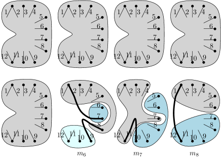
Figure 10: The matchings giving a $B$ set. The unmatched half-edges $3,4,5,6$ then form the vector $z$ and in this graph context would connect to the deleted vertex $v$.

Applying $\alpha$ to this $(m,z)$ we obtain $f$ with $f(1)=f(12)=8,f(2)=1,f(3)=2,f(4)=3,f(5)=4,f(6)=5,f(7)=f(8)=f(9)=6,f(10)=f(11)=7$ as illustrated in fig. 11.

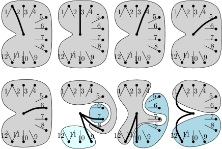
Figure 11: The systems of distinct representatives given by $f$ illustrated in the context of $S$ as the $h$-neighbourhood of the central vertex $u$.

5.2 Diagonals and the Martin invariant

We apply the results of section 5.1 to show that the diagonal coefficient satisfies the Martin recurrence and hence with suitable normalization agrees with the Martin invariant.

Theorem 5.13.

Let $G$ be a $2k$-regular graph with $n$ vertices. Then for any vertex $v$ without self-loops,

$$\left[x_{1}\cdots x_{k(n-2)}\right]\widetilde{\Psi}_{G\setminus v}^{k}=k!\cdot\operatorname{\mathsf{M}}\left(G\right).$$ (5.4)

Proof.

By lemma 5.3 the left-hand side, $N_{k}(G\setminus v)$, is the number of ordered partitions $E=T_{1}\sqcup\ldots\sqcup T_{k}$ of the edge set $E$ of $G\setminus v$ into $k$ edge-disjoint spanning trees $T_{i}$.

If $G$ has a self-loop, then $\operatorname{\mathsf{M}}(G)=0$ and by hypothesis on $v$, $G\setminus v$ also has a self-loop and so $N_{k}(G\setminus v)=0$ since no spanning tree can include any self-loop. Therefore, (5.4) holds whenever $G$ has one or more self-loops.

From now on, assume that $G$ has no self-loops. Then $G$ must have at least two vertices. If $G$ has exactly 2 vertices, then $G\cong K_{2}^{[k]}$ is a $k$-fold edge with $k!\cdot\operatorname{\mathsf{M}}(G)=1$, see (2.7), and $G\setminus v$ is a single vertex without edges and thus $N_{k}(G\setminus v)=1$ from the partition $T_{1}=\ldots=T_{k}=\emptyset$. So (5.4) holds for $n=2$.

To complete the proof, we will show that the diagonal coefficient $N_{k}(G\setminus v)$ satisfies the Martin recurrence (1.1): Let $w\neq v$ be another vertex of $G$, then we will prove that

$$N_{k}(G\setminus v)=\sum_{\tau\in\mathcal{T}^{\prime}(w)}N_{k}(G_{\tau}\setminus v)$$ (5.5)

where $\mathcal{T}^{\prime}(w)$ is the subset of transitions at $w$ that does not create a self-loop at $v$. This induction step reduces (5.4) from $n$ to $n-1$ vertices: if $N_{k}(G_{\tau}\setminus v)=k!\cdot\operatorname{\mathsf{M}}(G_{\tau})$ is already known, then the right-hand side of (5.5) is $k!\cdot\operatorname{\mathsf{M}}(G)$. The transitions $\tau\in\mathcal{T}(w)\setminus\mathcal{T}^{\prime}(w)$ missing from (1.1) only produce graphs with $\operatorname{\mathsf{M}}(G_{\tau})=0$ due to self-loops at $v$.

We now prove (5.5). Let $S$ be the $h$-neighbourhood (see section 2) of $w$ in $G\setminus v$.

Let $T_{1},\ldots T_{k}$ be a partition of $E$ into spanning trees of $G\setminus v$. For each $T_{i}$, let $X_{i}=T_{i}\cap S$ and $X_{i}^{\prime}$ be the set of edges incident to $w$ which contain a half-edge of $X_{i}$. The remaining edges $F_{i}=T_{i}\setminus X_{i}^{\prime}$ determine a spanning forest of $G\setminus\{v,w\}$. Such a forest $F_{i}$ induces a partition $P_{i}$ of $S$ as follows: two half-edges from the $h$-neighbourhood of $w$ are in the same part of $P_{i}$ if the corresponding neighbours of $w$ are in the same component of $F_{i}$. Since $T_{i}=X_{i}^{\prime}\sqcup F_{i}$ and $X_{i}$ is in bijection with $X_{i}^{\prime}$, $X_{i}$ includes precisely one half-edge in each part of $P_{i}$, so it is an SDR of $P_{i}$. Since the $T_{i}$ partition $E$, the SDRs $X_{1},\ldots,X_{k}$ partition $S$. Conversely, given any list of forests $F_{i}$ that induce $P_{i}$, and any partition of $S$ into SDRs $X_{i}$ of $P_{i}$, then each $T_{i}$ formed by taking $F_{i}=X_{i}^{\prime}\sqcup F_{i}$ (where $X_{i}^{\prime}$ is again the set of edges which contain a half-edge of $X_{i}$) is a spanning tree of $G\setminus v$ and these trees partition $E$. Therefore, we can write

$$N_{k}(G\setminus v)=\sum_{P}\left\lvert A(P_{1},\ldots,P_{k})\right\rvert\cdot\left\lvert C(P_{1},\ldots,P_{k})\right\rvert \sharp$$ ()

as a sum over all ordered sequences $P=(P_{1},\ldots,P_{k})$ of partitions of $S$. Here $A$ is defined in (5.3) and counts the choices of $X_{i}$. To count the choices of $F_{i}$, we define $C(P)$ as the set of lists $(F_{1},\ldots,F_{k})$ of spanning forests $F_{i}\subseteq E^{\prime}$ of $G\setminus\left\{v,w\right\}$ such that each $F_{i}$ induces $P_{i}$, and such that all $F_{i}$ together form a partition of the edge set $E^{\prime}$ of $G\setminus\left\{v,w\right\}$.

Now consider a transition $\tau$ of $G$ at $w$. This is a matching of the $h$-neighbourhood of $w$ in $G$. This neighbourhood differs from $S$ by the $d=2k-|S|$ half-edges $e_{1},\ldots,e_{d}$ incident to $v$. Suppose additionally that $\tau$ does not create any self-loops at $v$. Then let $z=(z_{1},\ldots,z_{d})$ be the elements of $S$ which are paired in $\tau$ with $e_{1},\ldots,e_{d}$. Let $m$ be the perfect matching of $S\setminus\left\{z_{1},\ldots,z_{d}\right\}$ given by the rest of the transition. We can thus identify the set $\mathcal{T}^{\prime}(w)$ with pairs $(m,z)$ of a $d$-tuple $z$ and a matching $m$ of the above form. Note that the elements of $m$ are canonically identified with edges in $G_{\tau}\setminus v$, such that the edge set of $G_{\tau}\setminus v$ is the disjoint union of $E^{\prime}$ and $m$.

Let $T^{\prime}_{1},\ldots T^{\prime}_{k}$ be a partition of the edges of $G_{\tau}\setminus v$ into spanning trees. Similarly to before, we can decompose each $T^{\prime}_{i}=m_{i}\sqcup F_{i}$ into the edges $m_{i}=T^{\prime}_{i}\cap m$ that belong to $m$ and a spanning forest $F_{i}=T_{i}^{\prime}\setminus m_{i}$ of $G\setminus\left\{v,w\right\}$. Let $P_{i}$ be the partition of $S$ induced by $F_{i}$. Then $m_{i}$ defines a tree on $P_{i}$ in the sense explained before definition 5.9. Conversely, given any forest $F_{i}$ that induces $P_{i}$, together with a matching $m_{i}$ defining a tree on $P_{i}$, we obtain a spanning tree $T_{i}^{\prime}=F_{i}\sqcup m_{i}$ of $G_{\tau}\setminus v$. Therefore, we can write

$$\sum_{\tau\in\mathcal{T}^{\prime}(w)}N_{k}(G_{\tau}\setminus v)=\sum_{P}\left\lvert B(P_{1},\ldots,P_{k})\right\rvert\cdot\left\lvert C(P_{1},\ldots,P_{k})\right\rvert, \flat$$ ()

as a sum over sequences $P=(P_{1},\ldots,P_{k})$ of partitions of $S$. Here, $B(P)$ from definition 5.9 counts the choices of $\tau$ (that is, $m$ and $z$) and also the choice of partition $m=m_{1}\sqcup\ldots\sqcup m_{k}$; whereas $C(P)$ counts the spanning forest decompositions $E^{\prime}=F_{1}\sqcup\ldots\sqcup F_{k}$ as before.

By proposition 5.11, ($\sharp$ ‣ 5.2) and ($\flat$ ‣ 5.2) agree and hence we proved (5.5). ∎

Corollary 5.14.

For a $2k$-regular graph $G$ and a vertex $v$ without self-loops, $\operatorname{\mathsf{M}}(G)$ is equal to the number of partitions of the edge set of $G\setminus v$ into $k$ spanning trees.

This combinatorial interpretation, stated as theorem 1.3 in the introduction, follows from corollary 5.4. It is illustrated for the example $\operatorname{\mathsf{M}}(K_{4})=6$ in (1.6). The claim remains true even if there are self-loops at $v$, for then $\operatorname{\mathsf{M}}(G)=0$ but also $N_{k}(G\setminus v)=0$, because $G\setminus v$ must then have more than $kn$ edges (where $G$ has $n+2$ vertices) and hence does not admit partitions into $k$ spanning trees (each of which contains $n$ edges).

Remark 5.15.

From this point of view, the condition $\operatorname{\mathsf{M}}(G)>0$ is equivalent to the existence of an edge partition of $G\setminus v$ into spanning trees. Necessary and sufficient conditions for the existence of such a partition were given by Nash-Williams [52] and Tutte [64]. In fact, for our case of $2k$-regular graphs $G$, it follows easily from [52, Lemma 5] that $G\setminus v$ has $k$ edge-disjoint spanning trees if and only if $G$ is $2k$-edge connected. This gives an alternative proof of corollary 3.3, which says that $\operatorname{\mathsf{M}}(G)>0$ in this case. Also for more general graphs, the maximal number of edge-disjoint spanning trees is related to the edge-connectivity via upper and lower bounds [38, 43].

Corollary 5.16.

Let $G$ be a $2k$-regular graph with $n$ vertices, and let $v$ denote a vertex without self-loops. Then for every positive integer $r$,

$$\operatorname{\mathsf{M}}(G^{[r]})=\frac{(r!)^{k(n-2)}}{(kr)!}\big{[}x_{1}^{r}\cdots x_{k(n-2)}^{r}\big{]}\widetilde{\Psi}_{G\setminus v}^{kr}.$$ (5.6)

Proof.

Combine theorem 5.13 with lemma 5.6. ∎

Corollary 5.17.

For a $2k$-regular graph $G$ with $n\geq 3$ vertices and any positive integer $r$, the Martin invariant $\operatorname{\mathsf{M}}(G^{[r]})$ is an integer that is divisible by $(r!)^{k(n-3)}$.

Proof.

Combine lemma 5.7 with corollary 5.16. ∎

The identity (5.6) shows that the sequence $\operatorname{\mathsf{M}}(G^{\bullet})$ of Martin invariants of all duplications $G^{[r]}$ of a fixed graph encodes the diagonal coefficients of all powers of the Kirchhoff polynomial. These coefficients are related to each other by a difference equation:

Corollary 5.18.

For any $2k$-regular graph $G$, there exists an integer $d>0$ and univariate polynomials $P_{0},\ldots,P_{d}\in\mathbbm{Z}[t]$ with $P_{d}\neq 0$ such that, for all $r\geq 1$,

$$P_{0}(r)\cdot\operatorname{\mathsf{M}}\left(G^{[r]}\right)+P_{1}(r)\cdot\operatorname{\mathsf{M}}\left(G^{[r+1]}\right)+\ldots+P_{d}(r)\cdot\operatorname{\mathsf{M}}\left(G^{[r+d]}\right)=0.$$ (5.7)

Proof.

If a rational function $f(x_{1},\ldots,x_{m})$ of several variables is non-singular at $x=0$, then it has a Taylor expansion at $x=0$. The diagonal coefficients of this expansion define a univariate formal power series $\operatorname{Diag}(f)=\sum_{r\geq 0}z^{r}\left[x_{1}^{r}\cdots x_{m}^{r}\right]f$ called the diagonal of $f$. Such diagonals are $D$-finite functions [45], hence the sequence of diagonal coefficients is $P$-recursive [60] (namely it fulfils a polynomial recurrence).

Therefore, the diagonal coefficients $\operatorname{\mathsf{M}}(G^{[r]})\cdot(kr)!/(r!)^{k(n-2)}$ of the geometric series $f=1/(1-\widetilde{\Psi}_{G\setminus v})=\sum_{i\geq 0}\widetilde{\Psi}^{i}_{G\setminus v}$ fulfil a recurrence of the form (5.7). Multiplying this recurrence with $((r+d)!)^{k(n-2)}/(kr)!$ produces the claimed recurrence for $\operatorname{\mathsf{M}}(G^{[r]})$ alone, by the transformation $P_{i}(r)\mapsto P_{i}(r)\cdot[(r+i+1)\cdots(r+d)]^{k(n-2)}\cdot(kr+1)\cdots(kr+ki)$. ∎

5.3 Duality

As an application of the connection between the Martin invariant and diagonal coefficients, we can relate the Martin sequences of graphs that are planar duals of each other.

Suppose that $G$ is a graph with a plane embedding and $G^{\star}$ denotes the corresponding dual graph. Then the edges of $G$ are in canonical bijection with the edges of $G^{\star}$. Under this correspondence, a set of edges defines a spanning tree in $G$ precisely when its complement defines a spanning tree in $G^{\star}$. Therefore, we have

$$\Psi_{G^{\star}}=\widetilde{\Psi}_{G}.$$ (5.8)

Recall that the Martin invariant of a regular graph $G$ can be computed by the diagonal coefficient of the Kirchhoff polynomial of a decompletion $G\setminus v$. For two regular graphs $G_{1}$ and $G_{2}$ with vertex degrees $d_{1}$ and $d_{2}$, respectively, a duality $(G_{1}\setminus v)^{\star}\cong G_{2}\setminus w$ between decompletions implies that $(d_{1},d_{2})\in\left\{(3,6),(4,4),(6,3)\right\}$. This follows from the constraints on the edge- and vertex numbers imposed by regularity and duality. In such cases, (5.8) translates into a relation between the Martin sequences of $G_{1}$ and $G_{2}$.

Corollary 5.19.

If $G_{1}$ and $G_{2}$ are 4-regular graphs such that there exist vertices $v_{1}$ and $v_{2}$ without self-loops such that $G_{1}\setminus v_{1}$ is a planar dual of $G_{2}\setminus v_{2}$, then the Martin sequences $\operatorname{\mathsf{M}}(G_{1}^{\bullet})=\operatorname{\mathsf{M}}(G_{2}^{\bullet})$ agree.

Proof.

Let $n$ denote the number of vertices of $G_{1}$. Then $G_{1}\setminus v_{1}$ and $G_{2}\setminus v_{2}$ each have $n-1$ vertices, $m=2n-4$ edges, and $n-2$ loops. From (4.12) and (5.8) we see that

$$\left[x_{1}^{r}\cdots x_{m}^{r}\right]\widetilde{\Psi}_{G_{1}\setminus v_{1}}^{2r}=\left[x_{1}^{r}\cdots x_{m}^{r}\right]\Psi_{G_{2}\setminus v_{2}}^{2r}=\left[x_{1}^{r}\cdots x_{m}^{r}\right]\widetilde{\Psi}_{G_{2}\setminus v_{2}}^{2r}$$

and thus the claim follows from corollary 5.16. ∎

Corollary 5.20.

Let $G_{3}$ be a 3-regular graph and $G_{6}$ a 6-regular graph, such that there exist vertices $v$ and $w$, without self-loops, such that $G_{3}\setminus v$ is a planar dual of $G_{6}\setminus w$. Let $n$ denote the number of vertices of $G_{6}$. Then for every positive integer $r$, we have

$$\operatorname{\mathsf{M}}\left(G_{3}^{[2r]}\right)=\left(\frac{(2r)!}{r!}\right)^{3(n-2)}\operatorname{\mathsf{M}}\left(G_{6}^{[r]}\right).$$ (5.9)

Proof.

The graphs $G_{3}\setminus v$ and $G_{6}\setminus w$ each have $m=3(n-2)$ edges. Setting $(r,k)$ to $(2r,3/2)$ in (5.2), we find that $\operatorname{\mathsf{M}}(G_{3}^{[2r]})\cdot(3r)!=[(2r)!]^{m}\left[x_{1}^{2r}\cdots x^{2r}_{m}\right]\widetilde{\Psi}^{3r}_{G_{3}\setminus v}$ from theorem 5.13. From (4.12) and (5.8) we see that

$$\left[x_{1}^{2r}\cdots x_{m}^{2r}\right]\widetilde{\Psi}_{G_{3}\setminus v}^{3r}=\left[x_{1}^{2r}\cdots x_{m}^{2r}\right]\Psi_{G_{6}\setminus w}^{3r}=\left[x_{1}^{r}\cdots x_{m}^{r}\right]\widetilde{\Psi}_{G_{6}\setminus w}^{3r},$$

and thus the claim follows from corollary 5.16. ∎

Through theorem 4.1, the above dualities imply relations between the graph permanents. Those have been noted before, see [22, Proposition 28].

Remark 5.21.

The identity (5.8) extends beyond the realm of planar graphs $G$ to all matroids $M$ and their duals $M^{\star}$, if we replace “spanning tree of $G$” in the definition of $\widetilde{\Psi}_{G}$ and $\Psi_{G}$ by “basis of $M$”. The matroid polynomial $\widetilde{\Psi}_{M}$ thus defined is still linear in each variable, and its degree is the rank of $M$. The degree of $\Psi_{M}$ is the corank (formerly loop number) of $M$. The combinatorial interpretation from lemma 5.3 identifies the diagonal coefficient of $\widetilde{\Psi}_{M}^{k}$ with decompositions into bases. The existence of such decompositions has been characterized in [28, Theorem 1]. For regular matroids, $\widetilde{\Psi}_{M}$ is the determinant of a matrix, similar to the graph Laplacian (4.11).

Consequently, any function of the diagonal coefficient of $\widetilde{\Psi}_{M}$ is invariant under matroid duality, for all matroids in the domain of the function—not just cycle matroids of planar graphs. For example, the permanent of regular matroids is invariant under duality. This follows from section 4.4 or the matrix manipulations in [23], since those apply without change to regular matroids. For the $c_{2}$ invariant, the situation is less clear: its connection to the diagonal coefficient is known only in the presence of a 3-valent vertex, see remark 6.18. Moreover, invariance of $c_{2}$ under duality is not even known for all graphic matroids [27].

Remark 5.22.

An identity of Feynman periods called Fourier split was introduced in [39, §2]. It operates by taking a planar dual on one side of a 3-vertex cut in a decompletion $G\setminus v$. This identity also holds for the Martin invariant. The same proof strategy as in section 3.2 applies: the Martin recursion (1.1) at a vertex on the other side of the 3-vertex cut reduces the statement by induction to smaller graphs. The remaining base case is the ordinary duality relation (Fourier identity).

We hence conclude via theorems 4.1 and 6.2 that also the extended graph permanent and the $c_{2}$ invariant at primes respect the Fourier split identity.

6 $c_{2}$ invariant

For any power $q=p^{s}$ of a prime $p$, let $\mathbbm{F}_{q}$ denote the finite field with $q$ elements. Given any polynomial $P\in\mathbbm{Z}[x_{1},\ldots,x_{m}]$ in $m$ variables $x_{i}$, we denote by

$$\left\llbracket P\right\rrbracket_{q}=\big{|}\big{\{}x\in\mathbbm{F}_{q}^{m}\colon P(x)=0\big{\}}\big{|}\in\mathbbm{Z}_{\geq 0}$$

the number of points on the hypersurface $\left\{P=0\right\}$ over $\mathbbm{F}_{q}$. In the special case $P=\Psi_{G}$ of Symanzik polynomials (1.7) of graphs, the study of point-counts goes back to [61, 62]. For all graphs with less than 14 edges [57], the point-counting function is a polynomial,

$$q\mapsto\left\llbracket\Psi_{G}\right\rrbracket_{q}=\sum_{i=0}^{m}c_{i}(G)q^{i}. \ast$$ ()

Starting at 14 edges, there exist graphs whose point-count is not polynomial [24, 57]. In fact, point-counting functions of graph hypersurfaces $\left\{\Psi_{G}=0\right\}$ can be as complicated as the point-counting functions of any variety, as made precise and proved in [3].

Lemma 6.1.

Let $G$ be a graph with at least 3 vertices and at least 2 edges. Then for every prime power $q$, the point count $\left\llbracket\Psi_{G}\right\rrbracket_{q}$ is divisible by $q^{2}$.

Proof.

This is proved in [57, Corollary 2.8] and [13, Proposition-Definition 18] when $G$ is connected. If $G$ is disconnected, then $\Psi_{G}=0$ and hence $\left\llbracket\Psi_{G}\right\rrbracket_{q}=q^{m}$ where $m$ is the number of edges of $G$. ∎

We will only consider point-counts of graphs with $n\geq 3$ vertices and $m=2(n-1)$ edges, hence lemma 6.1 applies and we can write

$$\left\llbracket\Psi_{G}\right\rrbracket_{q}\equiv q^{2}\cdot c_{2}^{(q)}(G)\mod q^{3}$$ (6.1)

for well-defined residues $c_{2}^{(q)}(G)\in\mathbbm{Z}/q\mathbbm{Z}$. The $c_{2}$-invariant [57] is the sequence of these residues, one for each prime power, given by

$$c_{2}^{(q)}(G)\equiv\frac{\left\llbracket\Psi_{G}\right\rrbracket_{q}}{q^{2}}\mod q.$$ (6.2)

Our main result in this section extracts $c_{2}$ at primes from the Martin invariant:

Theorem 6.2.

Let $G$ be a $4$-regular graph with at least 6 vertices. Then for every vertex $v$ of $G$, and very prime $p$, we have

$$c_{2}^{(p)}(G\setminus v)\equiv\frac{\operatorname{\mathsf{M}}(G^{[p-1]})}{3p}\mod p.$$ (6.3)

In section 6.1 we give a proof for primes $p\neq 3$, by relating $c_{2}$ to the diagonal coefficients of powers of $\Psi_{G}$ as in section 5. In sections 6.2, 6.3 and 6.4 we present another proof, which is more technical, but which works for all primes—including $p=3$.

Remark 6.3.

The relation eq. 6.3 does not extend to prime powers. Only a few relations for $c_{2}$ are known at prime powers, see [33, 58, 25].

Corollary 6.4.

Let $G$ be a $4$-regular graph $G$ with at least 6 vertices, and let $v,w$ denote two vertices. Then $c_{2}^{(p)}(G\setminus v)\equiv c_{2}^{(p)}(G\setminus w)\mod p$ for all primes $p$.

This proves the completion conjecture, [13, Conjecture 4], for all prime fields. This conjecture is a special case of the stronger [13, Conjecture 5] from [57, Remark 2.11]:

Conjecture 6.5.

Whenever $\mathcal{P}(G_{1})=\mathcal{P}(G_{2})$ for two primitive $\phi^{4}$ graphs, then $c_{2}^{(q)}(G_{1})\equiv c_{2}^{(q)}(G_{2})\mod q$ for all prime powers $q$.

Here a graph $G$ is called primitive $\phi^{4}$ if it can be obtained from a cyclically 6-connected 4-regular graph $G^{\prime}$ by deleting a vertex: $G\cong G^{\prime}\setminus v$. We then call $G^{\prime}$ the completion of $G$, and we also say that $G$ is a decompletion of $G^{\prime}$, as originally defined in section 1.2. Every $\phi^{4}$ graph has a unique completion, but a 4-regular graph can have several non-isomorphic decompletions.

The completion identity $\mathcal{P}(G\setminus v)=\mathcal{P}(G\setminus w)$ for cyclically 6-connected 4-regular graphs $G$ is only one of several known period identities proved in [56]. The twist and duality identities lead to further special cases of 6.5. Combining our results on the Martin invariant (proposition 3.12 and corollary 5.19) with theorem 6.2, we also obtain proofs of the corresponding identities for $c_{2}$. Specifically, for all primes $p$:

• If $G_{1}$ is a twist of $G_{2}$, then $c_{2}^{(p)}(G_{1}\setminus v)\equiv c_{2}^{(p)}(G_{2}\setminus w)\mod p$.

• If $G$ is planar, and $G^{\star}$ a planar dual, then $c_{2}^{(p)}(G)\equiv c_{2}^{(p)}(G^{\star})\mod p$.

The duality relation was known previously, even for prime powers [25]. Our twist identity for $c_{2}$ is a new result, however our proof of the completion identity is arguably more significant. The completion conjecture has been repeatedly stated explicitly [13, 14] and has had many unsuccessful or only partially successful attempts at a proof.

To apply the main theorem, we use some divisibility properties, which we record here and which are proved in section 6.4. In corollaries 6.28 and 6.32 we show:

Lemma 6.6.

Let $G$ denote a 4-regular graph with at least 4 vertices. Then for every prime $p$, $\operatorname{\mathsf{M}}(G^{[p-1]})$ is divisible by $p$. For $p=3$ and at least 5 vertices, we also have that $\operatorname{\mathsf{M}}(G^{[2]})$ is divisible by $3^{2}$. Hence, the right-hand side of eq. 6.3 is well-defined.

In practice, for the purpose of computing $c_{2}^{(p)}$, one can simplify the Martin recursion and ignore all graphs that have a $\geq p$ fold edge:

Lemma 6.7.

If $G$ is $4r$-regular with $p=r+1$ prime, and $G$ has at least 6 vertices and at least one edge with multiplicity $p$ or more, then $\operatorname{\mathsf{M}}(G)$ is divisible by $p^{2}$ (or $p^{3}$ in the case $p=3$) and hence such a graph does not contribute to $c_{2}$.

Proof.

Lemma 6.27 shows that applying the Martin recurrence around either end of an edge with multiplicity $\geq p$ gives a factor divisible by $p$ multiplying the Martin invariant of each $G_{\tau}$. Applying the previous lemma to $\operatorname{\mathsf{M}}(G_{\tau})$ gives the result. ∎

Remark 6.8.

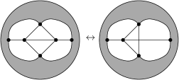
Figure 12: The double triangle operation.

The properties of the Martin invariant and theorem 6.2 also explain other $c_{2}$ identities which are known from [16] and [13, Corollary 34]:

• If $G$ has a 2-edge cut, a 4-edge cut, or a 3-vertex cut, then $c_{2}^{(p)}(G\setminus v)\equiv 0\mod p$.

• If $G$ and $G^{\prime}$ are related as in fig. 12, then $c_{2}^{(p)}(G)\equiv c_{2}^{(p)}(G^{\prime})\mod p$.

The first follows from theorem 1.2 and the factors of $p$ in $\operatorname{\mathsf{M}}(G^{[p-1]})$ (see lemma 6.6) producing $p^{2}$ in the products (1.3) and proposition 3.10. The double-triangle relation follows from lemma 6.7, since for either vertex incident to the edge shared between two triangles in $G$, after $(p-1)$-duplicating the only transitions that do not lead to self-loops or edges of multiplicity $p$ or larger, are precisely those that produce $G^{\prime}$.

We can exploit lemma 6.7 to simplify the calculation of $c_{2}^{(p)}$ in recursive families of graphs. A recursive family [19, §5] is in the simplest case a sequence $G_{1},G_{2},\ldots$ of graphs where $G_{n+1}$ is obtained from $G_{n}$ through a fixed local modification that affects only a finite number of vertices (call these the active vertices).

Lemma 6.9.

For recursive families of $\phi^{4}$ graphs $G_{1},G_{2},\ldots$ the Martin invariants $\operatorname{\mathsf{M}}(G_{1}^{[r]}),\operatorname{\mathsf{M}}(G_{2}^{[r]}),\ldots$ for a fixed integer $r$ fulfil a linear recurrence with constant coefficients.

Proof.

Applying the Martin recurrence to the finite number of vertices in $G_{n}$ that are involved in moving from $G_{n-1}$ to $G_{n}$ produces a linear combination of finitely many graphs which have the same recursive structure as $G_{n-1}$ and the same active vertices but with potentially different connections between the active vertices. The Martin recurrence can likewise be applied to these graphs and so on. There are only finitely many possibilities for connecting the active vertices so there are only finitely many such graphs to consider. Collecting the Martin invariants of these graphs into a vector $a_{n}$, we obtain a system of recurrences $a_{n}=Ta_{n-1}$ for some matrix $T$. ∎

For example, the prisms $K_{2}\times C_{n}$ can be constructed using 4 active vertices, by adding one rung at a time. We derive the corresponding recurrence for $\operatorname{\mathsf{M}}(G^{[2]}_{n})$ at the end of section 7.2. For the family of circulants $C_{1,2}^{n}$ we compute $\operatorname{\mathsf{M}}(G_{n})$ in (7.4).

Through theorem 6.2, the sequence $c_{2}^{(p)}(G_{n}\setminus v)$ at a fixed prime fulfils the same linear recurrence as $\operatorname{\mathsf{M}}(G^{[p-1]})$. Lemma 6.7 shows that we can drop all graphs with $\geq p$-fold edges from the vector $a_{n}$, to obtain a shorter recurrence for $c_{2}$. It could be interesting to compare this approach with the method of [68], since the latter produces recurrences that are considerably larger than necessary [70].

In order to prove theorem 6.2, we relate $c_{2}$ to diagonal coefficients of some polynomials. One such relation was known previously, and its combinatorial interpretation (lemma 6.14) was key to the results of [69, 40]. We will use this interpretation to prove theorem 6.2 for all primes, including $p=3$. For $p\neq 3$, we will also give a simpler proof using the diagonal coefficient of $\Psi$. We will need the following polynomials from [17]:

Definition 6.10.

Let $G$ be a graph and let $P$ be a partition of a subset of the vertices of $G$. The associated spanning forest polynomial is defined to be

$$\Phi_{G}^{P}=\sum_{F}\prod_{e\neq F}x_{e}$$

where the sum is over spanning forests $F$ of $G$ which are compatible with $P$ in the sense that there is a bijection between the trees of $F$ and the parts of $P$ such that each tree of $F$ contains all vertices that belong to the corresponding part of $P$.

Lemma 6.11.

Let $G$ be a 4-regular graph with at least 5 vertices and let $v$ and $w$ be two adjacent vertices, both without self-loops. Let $a,b,c$ be the three neighbours of $w$ which are not $v$ and let $x_{4},\ldots,x_{m}$ be the variables associated to the edges of $G\setminus\{v,w\}$. Then

$$c_{2}^{(p)}(G\setminus v)\equiv-\left[x_{4}^{p-1}\cdots x_{m}^{p-1}\right]{\left(\Phi^{\{a,b\},\{c\}}_{G\setminus\{v,w\}}\Psi_{G\setminus\{v,w\}}\right)^{p-1}}\mod p$$

for all primes $p$. Accordingly, the right-hand residue is invariant when permuting $a,b,c$.

Proof.

This is a consequence of a chain of results from [13] and [16]. To see them all laid out in detail to obtain the statement of the lemma, see [33, §2]. ∎

Remark 6.12.

With $G$ as in the lemma, and with $1,2,3$ the edges from $w$ to $a,b,c$ respectively, then the two spanning forest polynomials in the lemma can also be written in terms of Dodgson polynomials, which were introduced in [11]. Specifically

$$\Phi^{\{a,b\},\{c\}}_{G\setminus\{v,w\}} =\Psi_{G\setminus v,3}^{1,2}$$

$$\Psi_{G\setminus\{v,w\}} =\Psi_{G\setminus v}^{13,23}.$$

Proving these two facts is one of the steps in the chain of results proving the lemma, coming from results of [16] (see also example 2 of [33] or section 2.2 of [40] for the calculation exhibited pedagogically). We will not need to use Dodgson polynomials in the present paper, so we will not give their definition, but may use the two displayed above simply as an alternate notation for the corresponding spanning forest polynomials.

Definition 6.13.

For a graph $H$ with 3 vertices marked $a,b,c$ and an integer $r$ define $N_{r,r}(H)$ to be the number of ordered partitions of the set of edges of $H$ into $2r$ parts, the first $r$ of which are spanning trees of $H$, and the last $r$ of which are spanning forests compatible with the partition $\left\{\{a,b\},\{c\}\right\}$.

The following combinatorial interpretation of $c_{2}$ was proven and put to productive use in [69, 40, 33]. It will be used in our second proof of theorem 6.2.

Lemma 6.14.

Let $G$ be as in lemma 6.11. Then for every integer $r$,

$$\left[x_{4}^{r}\cdots x_{m}^{r}\right]\left(\Phi^{\{a,b\},\{c\}}_{G\setminus\{v,w\}}\Psi_{G\setminus\{v,w\}}\right)^{r}=N_{r,r}(G^{[r]}\setminus\left\{v,w\right\}).$$

Consequently, $c_{2}^{(p)}(G\setminus v)\equiv-N_{r,r}(G^{[r]}\setminus\left\{v,w\right\})\mod p$ for every prime $p=r+1$.

Proof.

For the first claim, apply the argument from the proof of lemma 5.3 to the left-hand side, using the observation from remark 5.5 that taking the complement of each part does not change the count. The second claim is then a corollary of lemma 6.11. ∎

Example 6.15.

To compute $c_{2}^{(2)}(G)$, the recursion has only 3 terms, which are again 4-regular graphs, hence we get a simple recursion as in (1.2):

$$c_{2}^{(2)}\Bigg{(}\vbox{\hbox{\includegraphics[scale={0.4}]{graphs/circstu0}}}\Bigg{)}\equiv c_{2}^{(2)}\Bigg{(}\vbox{\hbox{\includegraphics[scale={0.4}]{graphs/circstus}}}\Bigg{)}+c_{2}^{(2)}\Bigg{(}\vbox{\hbox{\includegraphics[scale={0.4}]{graphs/circstut}}}\Bigg{)}+c_{2}^{(2)}\Bigg{(}\vbox{\hbox{\includegraphics[scale={0.4}]{graphs/circstuu}}}\Bigg{)}\mod 2.$$ (6.4)

This can also be easily derived from a denominator identity as follows. Let $G$, $G_{s}$, $G_{t}$, $G_{u}$ be the four graphs in the order illustrated. To make use of the denominator identity we need a little bit of language of denominator reduction (see [11]): we will speak of denominators of graphs after reducing certain edges. These are essentially the denominators of the Feynman periods after integrating the variables corresponding to the edges, but crucially can be defined by purely algebraic means; this is the central observation of denominator reduction. The third denominator is the expression $\Psi^{13,23}\Psi^{1,2}_{3}$ used above. Denominators starting from the third can be used to compute $c_{2}$ by taking the point count (and a sign which alternates for each edge that is reduced). This is one of the lemmas that goes into the proof of lemma 6.11. Additionally, the second denominator is always a square, say $f^{2}$, and for any additional edge $e$ the third denominator is obtained from the second by $(\left[x_{e}^{1}\right]f)(\left[x_{e}^{0}\right]f)$, while whenever a denominator is a product $fg$ with $f\neq g$ the next denominator can be computed by taking the resultant $[f,g]_{e}$ where $e$ is any edge for which $f$ and $g$ are both linear in $x_{e}$. We will use the compressed notation $f^{e}$ for $\left[x_{e}^{1}\right]f$ and $f_{e}$ for $\left[x_{e}^{0}\right]f$ whenever $f$ is linear in $x_{e}$.

As described at the beginning of section 6.1 of [16], the square roots of the denominators after reducing the two explicitly drawn edges of $G_{s}$, $G_{t}$, and $G_{u}$ are given by $(A-B)$, $(B-C)$, and $(C-A)$ respectively where $A$, $B$, and $C$ are certain explicit spanning forest polynomials. Furthermore letting $e$ be any edge in the common part of $G,G_{s},G_{t}$, and $G_{u}$, by lemma 42 of [16]), the denominator after reducing the 4 illustrated edges of $G$ along with edge $e$ is equal to

$$[A,B]_{e}+[B,C]_{e}+[C,A]_{e}$$

Computing the third denominator for $G_{s}$ we get $(A-B)^{e}(A-B)_{e}=A^{e}A_{e}+B^{e}B_{e}-A^{e}B_{e}-A_{e}B^{e}=A^{e}B_{e}+B^{e}A_{e}-[A,B]_{e}+2A_{e}B^{e}$. Adding the third denominators for $G_{s}$, $G_{t}$, and $G_{u}$ we get

$$2A^{e}A_{e}+2B^{e}B_{e}+2C^{e}C_{e}-[A,B]_{e}-[B,C]_{e}-[C,A]_{e}-2A_{e}B^{e}-2B_{e}C^{e}-2C_{e}A^{e}$$

$$\equiv[A,B]_{e}+[B,C]_{e}+[C,A]_{e}\mod 2.$$

So the fifth denominator of $G$ equals modulo $2$ the sum of the third denominators of $G_{s}$, $G_{t}$, and $G_{u}$, but since denominators from the third on up compute $c_{2}$, by taking the diagonal coefficient (point count $\mod p$) we obtain

$$c_{2}^{(2)}(G)\equiv c_{2}^{(2)}(G_{s})+c_{2}^{(2)}(G_{t})+c_{2}^{(2)}(G_{u})\mod 2$$

as desired. This provides a very efficient recurrence to compute $c_{2}^{(2)}$ and gives a short alternative proof of [40]. In fact, this relation between the Martin invariant and $c_{2}$ at $p=2$ was the starting point that ultimately led to the result below for arbitrary primes.

6.1 Primes $p\neq 3$ from the diagonal

Lemma 6.16.

Consider a graph $G$ with $n\geq 4$ vertices and $m=2(n-1)$ edges. Let $p=r+1$ be prime. Then the diagonal coefficient of $\Psi_{G}^{2r}$ fulfils

$$\left[x_{1}^{r}\cdots x_{m}^{r}\right]\Psi_{G}^{2r}\equiv-3p^{2}\cdot c_{2}^{(p)}(G)\mod p^{3}.$$ (6.5)

Remark 6.17.

Figure 13: This graph shows the necessity of requiring at least 4 vertices in lemma 6.16.

The lemma fails for graphs with less than $4$ vertices: The graph $G$ in fig. 13 has $\left\llbracket\Psi_{G}\right\rrbracket_{q}=q^{3}$ and thus $c_{2}^{(p)}(G)\equiv 0$, whence the right-hand side is $0\mod p^{3}$. This point-count of $\Psi_{G}=x_{1}x_{2}+(x_{1}+x_{2})(x_{3}+x_{4})$ is obtained using [62, 57]. The diagonal coefficient of $\Psi_{G}^{2r}$ on the left-hand side, however, is equal to $\binom{2r}{r}^{2}\equiv p^{2}\mod p^{3}$.

Proof.

Pick a 3-valent vertex $w$, let $1,2,3$ be its incident edges, and let $a,b,c$ denote the vertices on the other ends of these edges. Then the spanning forest polynomials denoted

$$f_{0}=\Psi_{G\setminus w},\quad f_{1}=\Phi_{G\setminus w}^{\{a\},\{b,c\}},\quad f_{2}=\Phi_{G\setminus w}^{\{a,c\},\{b\}},\quad f_{3}=\Phi_{G\setminus w}^{\{a,b\},\{c\}},\quad f_{123}=\Phi_{G\setminus w}^{\{a\},\{b\},\{c\}}$$

are subject to $f_{0}f_{123}=f_{1}f_{2}+f_{1}f_{3}+f_{2}f_{3}$ [13, Lemma 22]. Furthermore, we have

$$\Psi_{G}=f_{0}(x_{1}x_{2}+x_{1}x_{3}+x_{2}x_{3})+x_{1}(f_{2}+f_{3})+x_{2}(f_{1}+f_{3})+x_{3}(f_{1}+f_{2})+f_{123}.$$

This implies $f_{0}\Psi_{G}=y_{1}y_{2}+y_{1}y_{3}+y_{2}y_{3}$ with $y_{i}=f_{0}x_{i}+f_{i}$. Expanding the trinomial,

$$f_{0}^{2r}\Psi_{G}^{2r}=\sum_{i+j+k=2r}\binom{2r}{i,j,k}(f_{0}x_{1}+f_{1})^{j+k}(f_{0}x_{2}+f_{2})^{i+k}(f_{0}x_{3}+f_{3})^{i+j}$$

and then extracting the coefficient of $x_{1}^{r}x_{2}^{r}x_{3}^{r}$, we see that if $f_{0}\neq 0$ then we can cancel $2r$ powers of $f_{0}$ from each side and get

$$\left[x_{1}^{r}x_{2}^{r}x_{3}^{r}\right]\Psi_{G}^{2r}=f_{0}^{r}\sum_{i+j+k=2r}\binom{2r}{i,j,k}\binom{i+j}{r}\binom{i+k}{r}\binom{j+k}{r}f_{1}^{r-i}f_{2}^{r-j}f_{3}^{r-k}.$$

This identity remains true when $f_{0}=0$, because in this case, the left-hand side vanishes because $\Psi_{G}^{2r}$ has degree $2r$ in the variables $x_{1},x_{2},x_{3}$.

Note that the first binomial coefficient is always divisible by $p$. The second binomial is divisible by $p$ when $k<r$ (so that $r<i+j=2r-k$), and similarly the remaining binomials are divisible by $p$ when $j<r$ and $i<r$, respectively.

In conclusion, the summand is divisible by $p^{3}$ unless two summation indices are equal to $r$. Therefore, only the indices $(i,j,k)\in\left\{(0,r,r),(r,0,r),(r,r,0)\right\}$ contribute $\mod p^{3}$:

$$\left[x_{1}^{r}x_{2}^{r}x_{3}^{r}\right]\Psi_{G}^{2r} \equiv\binom{2r}{r}^{2}\left((f_{0}f_{1})^{r}+(f_{0}f_{2})^{r}+(f_{0}f_{3})^{r}\right)\mod p^{3}$$

$$\equiv p^{2}\left((f_{0}f_{1})^{r}+(f_{0}f_{2})^{r}+(f_{0}f_{3})^{r}\right)\mod p^{3}.$$

Now take the diagonal coefficient $\left[x_{4}^{r}\cdots x_{m}^{r}\right]$ in the remaining variables, on both sides. Since each of the three products $f_{0}f_{i}$ is the polynomial on the right-hand side of lemma 6.11 for some permutation of $\left\{a,b,c\right\}$, the claim follows. ∎

This result converts the diagonal coefficient of the more complicated polynomials of lemma 6.11 into the diagonal coefficient of $\Psi^{2r}$—at least modulo $p^{3}$. For $p\neq 3$, by theorem 5.13, we thus obtain the desired relationship between the Martin invariant and the $c_{2}$ invariant. This proves theorem 6.2 for all primes $p\neq 3$.

Unfortunately, the explicit factor $3$ in lemma 6.16 does not allow us to draw the same conclusion when $p=3$. In this case we would need the congruence in lemma 6.16 to hold modulo $p^{4}$. Lacking a direct method to establish this congruence, we prove theorem 6.2 for $p=3$ using a different approach, detailed in the following subsections. The essence of this second proof is to avoid the troublesome explicit 3 appearing in lemma 6.16 by instead recreating the argument used in theorem 5.13 directly on the polynomials of lemma 6.11 using lemma 6.14. This second proof applies for all primes, although even there the case $p=3$ requires some special treatment in the base case of the induction.

As a consequence of this second proof, having established theorem 6.2 for $p=3$ we can infer indirectly that indeed, for $p=3$ the statement of lemma 6.16 holds modulo $p^{4}$, provided that $G$ has at least $8$ edges and $5$ vertices.

Remark 6.18.

The $c_{2}$ invariant and the diagonal coefficient of $\widetilde{\Psi}$ are defined for arbitrary graphs (with at least 5 edges and 4 vertices, say). It thus makes sense to ask if the statement of lemma 6.16 holds more generally. Note that our proof requires the existence of a $3$-valent vertex, which may not exist in more general graphs. Almost nothing is known, however, for $c_{2}$ invariants for graphs without 3-valent vertices. The only paper making a dent in this direction is [26].

6.2 Structure of the proof for all primes

Our second proof of Theorem 6.2 proceeds by showing that the diagonal coefficient $N_{r,r}$ from lemma 6.14 is congruent to the Martin invariant. Concretely, we will show that

$$-N_{r,r}(G\setminus\left\{v,w\right\})\equiv\frac{\operatorname{\mathsf{M}}(G)}{3p}\mod p$$ (6.6)

for every prime $p=r+1$ and every $4r$-regular graph $G$ with at least 6 vertices, provided $w$ is a vertex with four neighbours $\left\{a,b,c,v\right\}$, each connected to $w$ by an $r$-fold multiedge. Applied to the special case where $G$ is the $r$-fold duplication of a 4-regular graph, we obtain theorem 6.2 as the consequence of lemma 6.14. This approach works for all primes $p$ and thus fills the gap at $p=3$, which is not covered by the method of section 6.1.

The key step to prove (6.6) is to establish the Martin recurrence (1.1) for the left-hand side. Like the diagonal coefficient $N_{k}$ of $\Psi^{k}$ from section 5—see (5.5)—the diagonal coefficient $N_{r,r}$ also satisfies the Martin recurrence exactly: For a vertex $u\notin\left\{v,w,a,b,c\right\}$,

$$N_{r,r}(G\setminus\left\{v,w\right\})=\sum_{\tau\in\mathcal{T}^{\prime}(u)}N_{r,r}(G_{\tau}\setminus\left\{v,w\right\})$$ (6.7)

is the sum over all transitions at $u$ which do not produce a self-loop at $v$. The residue modulo $p$ in (6.6) is needed only to connect $N_{r,r}$ with $\operatorname{\mathsf{M}}(G)$ in the base cases (section 6.4), and with the $c_{2}$ invariant when $G$ is the $r$-fold duplication of a 4-regular graph.

At its core the idea to prove (6.7) is the same as for theorem 5.13, namely we interpret a transition as going from sets counted by $A$ (5.3) to those counted by $B$ (definition 5.9) and then use the Prüfer based proposition 5.11. However, this is more intricate for $N_{r,r}$ than for $N_{k}$, since we are now counting partitions of the edges into $r$ trees and $r$ forests consisting of two trees each, one containing $\left\{a,b\right\}$ and the other containing $\left\{c\right\}$. We thus need to keep track of where the marked vertices $\left\{a,b,c\right\}$ are. This requires augmenting the constructions of the proof of theorem 5.13 by 3 coloured vertices.

As in the proof of theorem 5.13, applying the recurrence (1.1) will lead us outside the world of $r$-duplicated graphs and we need to consider arbitrary graphs with the same vertex degrees. To this end, by $H$ we denote a graph with

• two vertices ($a$ and $b$) marked with one colour, say red, and one ($c$) with a second colour, say blue, all three of which have degree at most $3r$,

• all other vertices have degree at most $4r$, and

• the number of edges is $r(2n-3)$, where $n$ is the total number of vertices of $H$.

Then let $G$ be the graph obtained from $H$ by adding a new vertex $w$ with $r$ edges to each of the three coloured vertices of $H$, then adding a new vertex $v$ with $r$ edges to $w$ and edges to each remaining vertex of degree less than $4r$ so as to raise the degree to $4r$, and finally forgetting the colours. The above conditions on $H$ ensure that $G$ is $4r$-regular, $v$ and $w$ have no self-loops, and $H=G\setminus\left\{v,w\right\}$. Setting $H_{\tau}=G_{\tau}\setminus\left\{v,w\right\}$, we can state (6.7) as $N_{r,r}(H)=\sum_{\tau}N_{r,r}(H_{\tau})$.

Consequently, the structure of our inductive proof is as follows: we first show the Martin recurrence (6.7) for the number of partitions of edges of $H$ into $r$ spanning trees and $r$ spanning forest compatible with the colouring in section 6.3. Then in section 6.4 we compute these numbers when $H$ has only the three coloured vertices, and compare them with the Martin invariant of the corresponding graph $G$. This completes our second proof of theorem 6.2 and in particular proves the theorem in the case $p=3$.

6.3 Proof of the recurrence for all primes

Let $H$, $G$, $v$, $w$, and $r$ be as in section 6.2. In this section, we prove the recurrence (6.7).

Recall the definitions of $h$-neighbourhood and $v$-neighbourhood from section 2. Throughout this section, let $u$ be an uncoloured vertex of $H$, and $S$ its $h$-neighbourhood in $H$.

Given a partition of the edges of $H$ into $r$ spanning trees and $r$ spanning forests compatible with the vertex colours, consider what happens when we remove $u$. As in the proof of theorem 5.13, for each spanning tree, if $u$ has degree $k$ in the tree then upon removing $u$ the tree is split into $k$ trees and this induces a partition of $S$ into $k$ parts. For each spanning forest, the vertex $u$ is in one of the trees of the forest and if $u$ has degree $k$ in that tree, then upon removing $u$ this tree is split into $k$ trees and the other tree of the forest is unchanged, leaving a spanning forest of $k+1$ trees of $H\setminus u$. There are then two possibilities for the resulting induced partition of the $h$-neighbourhood $S$ of $u$: if all the vertices of the $v$-neighbourhood of $u$ were originally in the same tree as $u$, then locally around $u$ we only see one tree and so we get a partition of the $h$-neighbourhood $S$ of $u$ into $k$ parts as before. However, if some of the $v$-neighbourhood of $u$ was originally in the other tree, then there will additionally be a $(k+1)$th part in the induced partition of the $h$-neighbourhood corresponding to the other tree. In order to keep track of this we will need to introduce coloured partitions in this case.

We will first consider the case where for all the $r$ spanning forests the whole $v$-neighbourhood of $u$ is in the same tree. Here the local situation is exactly as for theorem 5.13 and so the same argument applies. We now briefly go through this argument again in order to set notation that will be useful when both trees interact around $u$.

Given a partition $P$ of the $h$-neighbourhood of $u$, say a spanning forest is compatible with both $P$ and the vertex colouring if it has $|P|+1$ trees, one of which involves all vertices of one colour and no vertices of $P$ or of the other colour and where the remaining $|P|$ trees are compatible with $P$. As observed in the proof of theorem 5.13, given a partition $P$ be a partition of the $h$-neighbourhood of $u$, any spanning forest of $H\setminus u$ compatible with $P$ can be extended to a spanning tree $T$ by choosing an SDR for $P$ and then adding the edges containing each of these half edges in $H$ to $T$; likewise for any spanning forest of $H\setminus u$ compatible with $P$ and the vertex colouring. Every spanning tree or spanning forest which induces the partition $P$ on the $h$-neighbourhood of $u$ is obtained in this way.

We call such an SDR a $u$-extension of $P$.

For the other side of the Martin recurrence, given a transition $\tau$ of $G$ which does not create self-loops at $v$, write $H_{\tau}$ for the graph obtained by applying the transition restricted to $H$ and removing the unmatched half-edges (those that were matched to $v$ in $G$). On each $H_{\tau}$ we are then counting partitions of the edges into $r$ spanning trees and $r$ spanning forests compatible with the coloured vertices. By breaking the edges matched by $\tau$, each such tree or forest induces a partition on the $v$-neighbourhood of $u$. For such a spanning forest, if all of the $v$-neighbourhood of $u$ is in the same tree of the forest, then locally we are only working with trees and so as in theorem 5.13 for any partition $P$ of the $h$-neighbourhood of $u$ with at most $\deg(u)-2r+1$ parts, any matching that defines a tree on $P$ in the sense of definition 5.9 serves to extend any spanning forest of $H\setminus u$ compatible with $P$ or compatible with $P$ and the vertex colouring. Furthermore, every such matching comes from at least one transition $\tau$ with no self loops at $v$ since the constraint on the number of parts guarantees enough half edges left to connect to $v$ without loops, and every spanning tree or spanning forest with all of the $v$-neighbourhood of $u$ is obtained in this way.

We call such a choice of matching an $m$-extension of $P$.

Let $S$ be the $h$-neighbourhood of $u$ in $H$ and let $P_{1},\ldots,P_{2r}$ be partitions of $S$. For $H^{\prime}=H$ or $H^{\prime}=H_{\tau}$ for some transition at $u$, write $N_{H^{\prime}}(P_{1},\ldots,P_{2r})$ for the number of partitions of the edges of $H^{\prime}$ into $r$ spanning trees and $r$ spanning forests compatible with the coloured vertices so that the $i$th spanning tree induces the same partition on the $v$-neighbourhood of $u$ that $P_{i}$ does and the $j$th spanning forest induces the same partition on the $v$-neighbourhood of $u$ that $P_{r+j}$ does and only one tree of the spanning forest is involved in the induced partition. Then what we need from theorem 5.13 is the following:

Proposition 6.19.

Let $P_{1},\ldots,P_{2r}$ be partitions of the $h$-neighbourhood of $u$ in $H$. Then

$$N_{H}(P_{1},\ldots,P_{2r})=\sum_{\tau}N_{H_{\tau}}(P_{1},\ldots,P_{2r})$$

where the sum is over transitions $\tau$ of $u$ in $G$ which do not create self loops at $v$.

Proof.

Consider spanning forests $F_{i}$ compatible with $P_{i}$ on $H\setminus u$ for each $1\leq i\leq r$ and spanning forests $F_{j}$ for each $p\leq i\leq 2r$ so $F_{j}$ has $|P_{j}|+1$ trees of which $|P_{j}|$ of them are compatible with $P_{j}$ and also contain the vertices of one of the two colours and the last tree contains the vertex of the other colour. Let $C(P_{1},\ldots,P_{2r})$ be the set of possible choices for the $F_{i}$.

If $\sum_{i=1}^{2r}|P_{i}|=\deg(u)$ and each partition has at most $\deg(u)-2r+1$ parts, then as in theorem 5.13

$$N_{H}(P_{1},\ldots,P_{2r})=\left\lvert C(P_{1},\ldots,P_{2r})\right\rvert\cdot\left\lvert A(P_{1},\ldots,P_{2r})\right\rvert$$

and collecting the sets of $m$-extensions by their $z$s,

$$\sum_{\tau}N_{H_{\tau}}(P_{1},\ldots,P_{2r})=\left\lvert C(P_{1},\ldots,P_{2r})\right\rvert\cdot\left\lvert B(P_{1},\ldots,P_{2r})\right\rvert$$

where the sum is over transitions $\tau$ of $u$ in $G$ which do not create self loops at $v$. Here we have used that for $\tau$ to have no self loops at $v$ we must have $|z|=\deg(u)-\sum_{i=1}^{r}2(|P_{i}|-1)=4r-\deg(u)$ which is the same condition as $\sum_{i=1}^{2r}|P_{i}|=\deg(u)$. Applying Proposition 5.11

$$N_{H}(P_{1},\ldots,P_{2r})=\sum_{\tau}N_{H_{\tau}}(P_{1},\ldots,P_{2r})$$

as desired.

Finally if $\sum_{i=1}^{2r}|P_{i}|\neq\deg(u)$ or some partition has more than $\deg(u)-2r+1$ parts then both sides are $0$: the left side because the $u$-extensions are SDRs and each $P_{i}$ has at least one part and the right side because all compatible transitions would have self loops at $v$. ∎

Now we extend this to the case where the $v$-neighbourhood of $u$ may involve both trees in one or more of the spanning forests. For such a spanning forest, the vertices of the $v$-neighbourhood of $u$ which were originally in the same tree as $u$ are now partitioned into $k$ parts, but there may additionally be a part containing vertices in the $v$-neighbourhood of $u$ which are in the other tree of the spanning forest. Furthermore, if the tree corresponding to the red vertices is the tree which contains $u$, then the two red vertices may be in the same tree after removing $u$ or they may be in two different trees after removing $u$. Thus, in the case that not all vertices of the $v$-neighbourhood of $u$ are in the same tree of the spanning forest, we need to mark the parts of the partition of the $v$-neighbourhood obtained by removing $u$ according to whether or not the tree associated to that part (after removing $u$) contained a red vertex or a blue vertex. This will result in one or two red parts, one blue part, and any other parts uncoloured. The partition of the $h$-neighbourhood is induced from the partition of the $v$-neighbourhood and also inherits the colours. Call this a coloured partition.

The extensions are now more intricate to describe:

Lemma 6.20.

Let $P$ be a coloured partition of the $h$-neighbourhood of a vertex $u$ of $H$ (that is $P$ has one or two parts marked as red, one part marked as blue, and the rest uncoloured). Any spanning forest of $H\setminus u$ compatible with $P$ can be extended to a spanning forest $F$ of $H$ where the red part(s) are in one tree and the blue part in the other tree by

• choosing one half edge from each red part of $P$ and each unmarked part of $P$ and then adding the edges containing each of these half edges in $H$ to $F$, or

• if there is only one red part in $P$, choosing one half edge from the blue part of $P$ and from each unmarked part of $P$ and then adding the edges containing each of these half edges in $H$ to $F$.

Every spanning forest of $H$ which is compatible with the coloured vertices of $H$ and which induces the coloured partition $P$ on the $h$-neighbourhood of $u$ is obtained in this way.

We again call such a choice of edges a $u$-extension of the coloured partition $P$.

Proof.

In any case, all uncoloured components must join through $u$ as otherwise we would have 3 or more trees in the final forest. If there are two red parts then they must join through $u$ in order to be connected and so only the first option is possible. With one red and one blue part we are free to join either one through $u$.

For coloured and uncoloured parts, the ways to join through $u$ are as in the tree case. ∎

Now consider the other side of a Martin-type recurrence. Given a transition $\tau$ of $u$ in $G$ which does not create self-loops around $v$ and with $H_{\tau}$ as before. A spanning forest of $H_{\tau}$ again results in a partition of the vertices of $H$ and hence the $h$-neighbourhood of $u$ and if both trees of the forest appear in the $h$-neighbourhood of $u$ then we need to mark the parts of the partition of the $h$-neighbourhood of $u$ red or blue if their tree contained a red or blue vertex after splitting all edges of the matching, resulting in a coloured partition of the $h$-neighbourhood of $u$.

Again we only need this local information to extend forests.

Lemma 6.21.

Let $u$ be an uncoloured vertex of $H$ and let $P$ be a coloured partition of the $h$-neighbourhood of $u$ with at most $\deg(u)-2r+2$ parts. Any spanning forest of $H\setminus u$ compatible with $P$ can be extended to a spanning forest $F$ of some $H_{\tau}$ where the red part(s) are in one tree and the blue part in the other tree by choosing a forest structure $X$ where the vertex set of $X$ is the set of parts of $P$ and the forest is compatible with the colours coming from the parts of $P$, and then for each end of an edge of $X$ choosing a distinct half edge from the corresponding part of $P$.

Every spanning forest of every $H_{\tau}$ which is compatible with the coloured vertices of $H$ and which induces the coloured partition $P$ on the $h$-neighbourhood of $u$ is obtained in this way.

We again call such a choice of edges an $m$-extension of the coloured partition $P$.

Proof.

As for the tree case but so as to obtain a compatible spanning forest. The condition on the number of parts likewise makes it always possible for $\tau$ to avoid self-loops at $v$ where the spanning forest structure on $X$ uses one fewer edge than the tree structure did. ∎

Extend the meaning of $N_{H}(P_{1},\ldots,P_{2r})$ where $P_{p},\ldots,P_{2r}$ may be coloured to be the number of partitions of the edges of $H$ into $r$ spanning trees and $r$ spanning forests compatible with the coloured vertices so that the $i$th spanning tree induces the same partition on the $v$-neighbourhood of $u$ that $P_{i}$ does and the $j$th spanning forest induces the same partition on the $v$-neighbourhood of $u$ that $P_{r+j}$ does, with the inherited colouring if multiple trees of the forest interact with the $v$-neighbourhood of $u$.

When some of the $P_{i}$ may be coloured partitions, we bootstrap off Proposition 6.19.

Proposition 6.22.

Let $P_{1},\ldots,P_{2r}$ be partitions of the $h$-neighbourhood of $u$ where for $p\leq i\leq 2r$ the partition $P_{i}$ may be a coloured partition. Then

$$N_{H}(P_{1},\ldots,P_{2r})=\sum_{\tau}N_{H_{\tau}}(P_{1},\ldots,P_{2r})$$

where the sum is over transitions $\tau$ of $u$ in $G$ which do not create self loops at $v$.

Proof.

Proposition 6.19 gives the result when all of the partitions are uncoloured and so we now reduce to that case.

With $P_{i}$ as in the statement, let $A(P_{1},\ldots,P_{2r})$, generalizing (5.3), denote the set of $u$-extensions for each $P_{i}$ (in the coloured sense where appropriate) which partition the edges of $H$ around $u$. Likewise, for each transition $\tau$ at $u$, let $B_{\tau}(P_{1},\ldots,P_{2r})$, generalizing definition 5.9, denote the set of $m$-extensions for each $P_{i}$ (in the coloured sense where appropriate) for which the union of the matchings gives the matching of $\tau$ on $S$.

We will show that

$$|A(P_{1},\ldots,P_{2r})|=\sum_{\tau}|B_{\tau}(P_{1},\ldots,P_{2r})|.$$ (6.8)

Multiplying by the number of possible choices for the forests in $H\setminus u$ which give $P_{i}$ will then give the result.

Suppose $P_{i}$ is a coloured partition with one red part and one blue part. For any $u$-extension of this coloured partition we take either an edge from the red part or an edge from the blue part and that choice is independent of the choices for the other parts. Therefore the $u$-extensions of the coloured partition $P_{i}$ are the same as the $u$-extensions of the uncoloured partition resulting from merging the red and blue parts of $P_{i}$ and then forgetting the colours. Similarly for any $m$-extension of $P_{i}$, we obtain a spanning forest on $P_{i}$ with two trees, one containing the vertex associated to the red part and one containing the vertex associated to the blue part. Merging the red and blue parts then the same edge and end information gives an $m$-extension of the uncoloured partition obtained from merging the red and blue parts and forgetting the colour and every such tree becomes a forest and a valid $m$-extension upon splitting this part to reobtain $P_{i}$. If $P_{i}$ had no more than $\deg(u)-2r+2$ parts before merging then it has no more than $\deg(u)-2r+1$ parts after, and vice versa.

Therefore, for the purposes of (6.8), whenever there is a coloured partition with one red and one blue part, merge those two parts and proceed with an uncoloured partition instead.

It remains to consider partitions with two red parts and one blue part. Suppose $P_{i}$ is such a partition and let $p$ be the blue part and $q$ and $s$ the two red parts. Similarly to the above, every $u$-extension of $P_{i}$ is also a $u$-extension after merging $p$ and $q$ and forgetting the colours, and is also a $u$-extension after merging $p$ and $s$ and forgetting the colours. However, merging $p$ and $q$ also allows $u$-extensions which use an edge from $p$ and an edge from $s$, and merging $p$ and $s$ also allows $u$-extensions which use an edge from $p$ and an edge from $q$. These are exactly the $u$-extensions obtained from merging $q$ and $s$ and forgetting the colours. Therefore, indicating the merged parts as superscripts, for example $P_{i}^{p\cup q}=(P_{i}\setminus\left\{p,q\right\})\cup\left\{p\cup q\right\}$, we see that

$$2|A(P_{1},\ldots,P_{i},\ldots,P_{2r})|\\ =|A(P_{1},\ldots,P_{i}^{p\cup q},\ldots,P_{2r})|+|A(P_{1},\ldots,P_{i}^{p\cup s},\ldots,P_{2r})|-|A(P_{1},\ldots,P_{i}^{q\cup s},\ldots,P_{2r})|$$

where the counts on the right hand side involve one coloured partition fewer than on the left hand side.

The situation is similar for the $m$-extensions. Every $m$-extension of $P_{i}$ is also an $m$-extension after merging $p$ and $q$ and forgetting the colours, and is also an $m$-extension after merging $p$ and $s$ and forgetting the colours. However, merging $p$ and $q$ also allows $m$-extensions where $s$ is in the tree with $p$ after re-splitting $p$ and $q$, and merging $p$ and $s$ also allows $m$-extensions where $s$ is in the tree with $q$ after re-splitting $p$ and $s$. These are exactly the $m$-extensions obtained from merging $q$ and $s$ and forgetting the colours. The bounds on the numbers of parts correspond as before. Therefore, for each $\tau$ we have

$$2|B_{\tau}(P_{1},\ldots,P_{i},\ldots,P_{2r})|\\ =|B_{\tau}(P_{1},\ldots,P_{i}^{p\cup q},\ldots,P_{2r})|+|B_{\tau}(P_{1},\ldots,P_{i}^{p\cup s},\ldots,P_{2r})|-|B_{\tau}(P_{1},\ldots,P_{i}^{q\cup s},\ldots,P_{2r})|$$

which lines up term by term with what was obtained for the $u$-extensions.

Similarly expanding for each remaining coloured partition, we can write $A(P_{1},\ldots,P_{2r})$ and the $B_{\tau}(P_{1},\ldots,P_{2r})$ for each $\tau$ as identical signed sums involving only uncoloured partitions of $S$.

Consider any pair of corresponding terms in the $A$ and $B$ sums: $|A(P_{1}^{\prime},\ldots,P_{2r}^{\prime})|$ and $|B_{\tau}(P_{1}^{\prime},\ldots,P_{2r}^{\prime})|$ where the $P_{i}^{\prime}$ are all uncoloured. We have $N_{H}(P_{1}^{\prime},\ldots,P_{2r}^{\prime})=\sum_{\tau}N_{H_{\tau}}(P_{1}^{\prime},\ldots,P_{2r}^{\prime})$ from proposition 6.19 and hence dividing by the number of possible choices for the forests in $H\setminus u$ which induce the $P_{i}^{\prime}$ gives $|A(P_{1}^{\prime},\ldots,P_{2r}^{\prime})|=\sum_{\tau}|B_{\tau}(P_{1}^{\prime},\ldots,P_{2r}^{\prime})|$. Therefore the expansions of $|A(P_{1},\ldots,P_{2r})|$ and $|B_{\tau}(P_{1},\ldots,P_{2r})|$ agree term by term proving (6.8) and hence proving the proposition. ∎

Summing both sides of proposition 6.22 over all choices of the partitions $P_{i}$, we obtain the Martin recursion $N_{r,r}(H)=\sum_{\tau}N_{r,r}(H_{\tau})$ as claimed in eq. 6.7.

6.4 Base cases

Recall that $p=r+1$ is prime. Given a graph $H$ with three marked vertices called $\left\{1,2,3\right\}$, with $(2|V(H)|-3)r$ edges, and with no vertex of degree more than $4r$, recall that $H$ determines a $4r$-regular graph $G$ by adding two vertices, labelled $\left\{v,w\right\}$, adding $r$ edges between $w$ and each of $\left\{1,2,3,v\right\}$, and finally adding $3r$ edges between $v$ and the original vertices of $H$ in the unique way such that the resulting graph $G$ is $4r$-regular. With this construction, $H=G\setminus\left\{v,w\right\}$.

Recall that $N_{r,r}(H)$ from definition 6.13 counts the ordered partitions of the edges of $H$ into $r$ spanning trees and $r$ spanning forests compatible with the partition $\{1,2\},\{3\}$.

For the base case of our inductive proof, we need to show that

$$-N_{r,r}(H)\equiv\frac{\operatorname{\mathsf{M}}(G)}{3p}\mod p$$ (6.9)

for all marked graphs $H$ as above on a fixed small number of vertices. The argument is easier for $G$ and $H$ smaller, and so for $p\neq 3$ we will prove (6.9) for $H$ with 3 vertices (only the marked vertices) and hence $G$ with 5 vertices. For $p=3$ we will need to move to $H$ with 4 vertices and hence $G$ with $6$ which remains sufficient for theorem 6.2.

Suppose, then, that $H$ is a marked graph with only 3 vertices—namely, the marked vertices—and $3r$ edges, and $G$ as above.

Consider first the left-hand side.

Lemma 6.23.

For any graph $H=G\setminus\left\{0,\infty\right\}$ with $3$ vertices and $3r$ edges and $p=r+1$ prime and $G$ as explained above, we have

$$-N_{r,r}(H)\equiv\begin{cases}1\mod p,&\text{if $G\cong K_{5}^{[r]}$, and}\\ 0\mod p,&\text{otherwise.}\\ \end{cases}$$ (6.10)

Proof.

Any self-loop in $H$ cannot belong to any tree or forest, hence forces $N_{r,r}(H)=0$. Thus suppose that $H$ has no self-loops. Let $n_{ij}$ denote the number of edges between vertices $i$ and $j$. The 2-forests of $H$ that separate $\left\{1,2\right\}$ from $\left\{3\right\}$ consist of a single edge between $1$ and $2$. Hence there are precisely $\binom{n_{12}}{r}$ ways to assign $r$ of these edges to 2-forests. The remaining edges are to be grouped into $a$ spanning trees of the form $\left\{12,13\right\}$, $b$ spanning trees $\left\{12,23\right\}$, and $c$ spanning trees $\left\{13,23\right\}$. The constraints $n_{12}-r=a+b$, $n_{13}=a+c$, and $n_{23}=b+c$ have the unique solution $a=r-n_{23}$, $b=r-n_{13}$, $c=2r-n_{12}$ where we note $a+b+c=r$. After choosing $a$ out of the $n_{12}-r$ edges $12$ and $a$ out of the $n_{13}$ edges $13$, there are $a!$ ways to pair them up into spanning trees of the first type, etc. Finally, accounting for the $r!$ ways to order the spanning trees and 2-forests, we find

$$N_{r,r}(H)=r!\binom{n_{12}}{r}r!a!b!c!\binom{n_{12}-r}{a}\binom{n_{13}}{a}\binom{n_{23}}{b}=\frac{r!\cdot n_{12}!\cdot n_{13}!\cdot n_{23}!}{a!b!c!}.$$ (6.11)

We need $n_{12}\geq r$ for $N_{r,r}(H)$ to be non-zero. Then $c\leq r$ and we always have $a,b\leq r$, hence the denominator is not divisible by $p$. So the numerator, and hence $N_{r}(H)$, become divisible by $p$ if any $n_{ij}>r$. For this not to happen, we need each $n_{ij}\leq r$. But then we must have $n_{12}=n_{13}=n_{23}=r$, due to the constraint $n_{12}+n_{13}+n_{23}=3r$. Then all edges in $G$ are $r$-fold, and we get $N_{r,r}(H)=(r!)^{3}\equiv-1\mod p$ by Wilson’s theorem. ∎

We now turn to the right-hand side of (6.9).

Consider the effect of multiedges on the expansion (1.1) of the Martin invariant at a vertex $v$ without self-loops. Let $w_{1},\ldots,w_{m}$ denote the neighbours of $v$, and say that there are $d_{i}$ edges $vw_{i}$ between $v$ and $w_{i}$. Then $G_{\tau}$ depends only on the numbers $D_{ij}$ of pairs $\left\{vw_{i},vw_{j}\right\}$ in $\tau$. Hence different transitions with the same numbers $D_{ij}$ will repeat the same contributions $\operatorname{\mathsf{M}}(G_{\tau})$.

Definition 6.24.

Let $D$ be a symmetric matrix $D$ of non-negative integers with diagonal $D_{ii}=0$ and row sums $\sum_{j}D_{ij}=d_{i}$ equal to the multiplicities of the edges between $v$ and its neighbours $w_{i}$. We write $G_{D}=G_{\tau}$ for any transition $\tau\in\mathcal{T}(v)$ with precisely $D_{ij}$ matches $\left\{vw_{i},vw_{j}\right\}$ between any pair of neighbours. We also introduce the notation

$$d!=d_{1}!\cdots d_{m}!\quad\text{and}\quad D!=\prod_{1\leq i<j\leq m}(D_{ij}!).$$

We only consider zero diagonals, because $D_{ii}>0$ would produce self-loops in $G_{D}$, which thus do not contribute to $\operatorname{\mathsf{M}}(G)$. The row sum constraint arises because a transition has to pair up all half-edges at $v$.

Lemma 6.25.

Let $G$ be a regular graph without self-loops and $v$ any vertex. Let $d=(d_{1},\ldots,d_{m})$ denote the edge multiplicities at $v$. Then

$$\operatorname{\mathsf{M}}(G)=\sum_{D}\frac{d!}{D!}\operatorname{\mathsf{M}}(G_{D})$$ (6.12)

where the sum is over all matrices $D$ as in definition 6.24. The coefficients are integers,

$$\frac{d!}{D!}=D!\prod_{i=1}^{m}\binom{d_{i}}{D_{i1},\ldots,D_{im}}.$$ (6.13)

Proof.

With the notation introduced above, this is just a rewriting of the vertex expansion (1.1), including only transitions that do not produce self-loops in $G_{\tau}$. The coefficient of $\operatorname{\mathsf{M}}(G_{D})$ is the number of transitions with the number of pairings prescribed by $D$. For every neighbour $w_{i}$, a transition partitions the $d_{i}$ edges $vw_{i}$ into a part of size $D_{i1}$ (which is paired with an edge $vw_{1}$), a part of size $D_{i2}$ (to be paired with $vw_{2}$), and so on. These partitions are counted by the multinomial coefficients in (6.13). The remaining factors $D_{ij}!$ in $D!$ count the ways to pair the thus chosen $D_{ij}$ copies of $vw_{i}$ with the $D_{ji}=D_{ij}$ chosen copies of $vw_{j}$ into the new edges $\left\{vw_{i},vw_{j}\right\}$ in $G_{D}$. ∎

Example 6.26.

Let $K_{4}^{[a,b,c]}$ denote the graph on 4 vertices with $n_{12}=n_{34}=a$, $n_{13}=n_{24}=b$, and $n_{14}=n_{23}=c$, where $n_{ij}$ denotes the number of edges between vertices $i$ and $j$. This is a regular graph of degree $a+b+c$. Suppose that $a+b+c=2k$ is even. Then there is at most a single summand in (6.12), because a matrix $D$ for the transitions at vertex $4$ is uniquely determined by the row sums $(d_{1},d_{2},d_{3})=(c,a,b)$; it must be $D_{12}=k-a$, $D_{13}=k-b$, $D_{23}=k-c$. Therefore

$$\operatorname{\mathsf{M}}\left(K_{4}^{[a,b,c]}\right)=\begin{cases}\frac{a!b!c!}{(k-a)!(k-b)!(k-c)!}&\text{if $a,b,c\leq k$ and}\\ 0&\text{otherwise.}\\ \end{cases}$$ (6.14)

Lemma 6.27.

If $p$ is a prime and $v$ a vertex with a neighbour $w_{i}$ with edge multiplicity $d_{i}\geq p$, then for every summand in (6.12), the coefficient $d!/D!$ is divisible by $p$.

Proof.

If $D$ has an entry $D_{ij}\geq p$, the divisibility follows from the $D!$ factor on the right-hand side of (6.13). So assume that all entries of $D$ are less than $p$. Then $D!$ is not divisible by $p$, but $d_{i}!$, and thus $d!/D!$, is. ∎

Corollary 6.28.

For every $4r$-regular graph $G$ on at least 4 vertices, with $p=r+1$ prime, $\operatorname{\mathsf{M}}(G)$ is divisible by $p$.

Proof.

If $G$ has self-loops, then the claim is trivial by $\operatorname{\mathsf{M}}(G)=0$. For graphs with more than 4 vertices, the claim follows inductively by vertex expansion (1.1) to smaller graphs. Hence we only need to consider $G$ with $4$ vertices and no self-loops, that is, $G\cong K_{4}^{[a,b,c]}$ for some integers $a,b,c$ with $a+b+c=4r$. Since at least one of $\left\{a,b,c\right\}$ must exceed $r=p-1$, the previous lemma implies the claim. ∎

Corollary 6.29.

Let $p=r+1$ be prime. Then for every $4r$-regular graph $G$ with 5 vertices, which is not isomorphic to $K_{5}^{[r]}$, we have that $\operatorname{\mathsf{M}}(G)$ is divisible by $p^{2}$.

Proof.

If $G$ has any edge of multiplicity greater than $r$, expansion at a vertex with such an edge writes $\operatorname{\mathsf{M}}(G)$ as a linear combination of $(d!/D!)\operatorname{\mathsf{M}}(G_{D})$. The factor $d!/D!$ is divisible by $p$ due to lemma 6.27, and $\operatorname{\mathsf{M}}(G_{D})$ is divisible by $p$ due to corollary 6.28. So we conclude that $\operatorname{\mathsf{M}}(G)$ is divisible by $p^{2}$ whenever $G$ has an edge with multiplicity $\geq p$. So, assume that all edges have multiplicity $\leq r$. To reach degree $4r$ at every vertex, we must then have $G\cong K_{5}^{[r]}$. ∎

Lemma 6.30.

The Martin invariant of the $r$-fold power of the complete graph $K_{5}$ is

$$\operatorname{\mathsf{M}}\left(K_{5}^{[r]}\right)=(r!)^{4}\sum_{a+b+c=r}\frac{(r+a)!(r+b)!(r+c)!}{(a!b!c!)^{2}(r-a)!(r-b)!(r-c)!}$$ (6.15)

and congruent to $\operatorname{\mathsf{M}}(K_{5}^{[r]})\equiv-3p\mod p^{2}$ whenever $p=r+1$ is prime.

Proof.

The expansion (6.12) at any vertex produces

$$\operatorname{\mathsf{M}}\left(K_{5}^{[r]}\right)=\sum_{a+b+c=r}\frac{r!r!r!r!}{(a!b!c!)^{2}}\operatorname{\mathsf{M}}\left(K_{4}^{[r+a,r+b,r+c]}\right).$$

Inserting (6.14) gives (6.15). Now consider $p=r+1$ prime. The denominator of the summand in (6.15) is not divisible by $p$. The numerator is divisible by $p^{2}$ unless at most one of $a,b,c$ is non-zero. We conclude that modulo $p^{2}$, only the three summands with $(a,b,c)\in\left\{(0,0,r),(0,r,0),(r,0,0)\right\}$ contribute. Therefore,

$$\operatorname{\mathsf{M}}\left(K_{5}^{[r]}\right)\equiv 3(r!)^{2}(2r)!=3(r!)^{3}p(p+1)\cdots(2p-2)\equiv-3p\cdot(r!)^{4}\mod p^{2}$$

and the claim follows from Wilson’s theorem $r!\equiv-1\mod p$. ∎

Note how the three explicit summands contributing in the last step of the proof are what leads to the explicit factor of $3$, causing extra trouble for $p=3$.

Corollary 6.31.

For every $4r$-regular graph with 5 vertices and $r+1$ prime, we have $\operatorname{\mathsf{M}}(G)\equiv-3pN_{r,r}(H)\mod p^{2}$.

Proof.

For every graph other than $K_{5}^{[r]}$ the claim follows from corollary 6.29 and lemma 6.23. For $G=K_{5}^{[r]}$, see lemma 6.30 and lemma 6.23. ∎

This establishes the base case (6.9) for all primes $p\neq 3$. Now consider the special case $p=3$. Then (6.9) is equivalent to

$$\operatorname{\mathsf{M}}(G)\equiv-9N_{2,2}(H)\mod 27,$$ (6.16)

that is, we have to compute the Martin invariants $\mod p^{3}$. We first note that the expression $\operatorname{\mathsf{M}}(G)/9\mod 3$ on the right-hand side of (6.9) makes sense.

Lemma 6.32.

The Martin invariant of every 8-regular graph with at least 5 vertices is divisible by $9$.

Proof.

By vertex expansion (1.1), the claim reduces to the case of graphs $G$ with $5$ vertices. If $G=K_{5}^{[2]}$, then $\operatorname{\mathsf{M}}(G)\equiv-3p\equiv 0\mod p^{2}$ for $p=3$. For all other graphs, see corollary 6.29. ∎

We thus have $\operatorname{\mathsf{M}}(G)\equiv-9m\mod 27$ for some integer $m$, but for graphs with $5$ vertices, $m$ is not necessarily equal to $N_{2,2}(H)$. For example, the totally decomposable graph

$$\operatorname{\mathsf{M}}\left(\vbox{\hbox{\includegraphics[scale={0.55}]{graphs/K5plus2}}}^{[2]}\right)=(4!)^{2}\equiv 9\mod 27$$

has $m\equiv-1\mod 3$; but we saw in lemma 6.23 that $N_{2,2}(H)\equiv 0\mod 3$. Therefore, for prime $p=3$ and $5$ vertices, the $c_{2}$ invariant cannot be read off the Martin invariant modulo $p^{3}$. We need to base the induction one step up, at 6 vertices.

So consider an $8$-regular graph $G$ with 6 vertices. Recall that $G$ has 5 special vertices labelled $\left\{v,w,1,2,3\right\}$ with $H=G\setminus\left\{v,w\right\}$, such that $w$ is connected only to $\left\{1,2,3,v\right\}$, via a double edge to each. It follows that the sixth vertex, call it $u$, is not connected to $w$ and has at most 4 neighbours $\left\{1,2,3,v\right\}$. If any of these connections to $u$ has multiplicity 3 or higher, then lemma 6.27 shows that $N_{2,2}(H)\equiv 0\mod 3$, since $N_{2,2}(H)$ fulfils the Martin recursion at $u$. By lemma 6.27 and lemma 6.32, we also find $\operatorname{\mathsf{M}}(G)\equiv 0\mod 27$, hence we have established (6.16) in this case.

It remains to consider graphs $G$ where $u$ is connected to each of $\left\{1,2,3,v\right\}$ via a double edge. So we are only left to arrange 8 edges between $\left\{1,2,3,v\right\}$ to obtain an 8-regular graph $G$. Let $n_{ij}$ denote these multiplicities. The 8-regularity implies that $n_{12}=n_{3v}$, $n_{13}=n_{2v}$, and $n_{1v}=n_{23}$. As before, any edge of multiplicity $n_{ij}\geq 3$ will force $\operatorname{\mathsf{M}}(G)\equiv 0\mod 27$. Similarly, we will have $N_{2,2}(H)\equiv 0\mod 3$, because the expansion at $u$ can only add further edges between $\left\{1,2,3\right\}$; so if $n_{1j}\geq 3$ already, it will stay above 2 even in $G_{D}\setminus\left\{v,w\right\}$, and therefore $N_{2,2}(H)\equiv 0\mod 3$ by lemma 6.23.

$G=\vbox{\hbox{\includegraphics[scale={0.5}]{graphs/octa2}}}$   $G^{\prime}=\vbox{\hbox{\includegraphics[scale={0.5}]{graphs/octa3}}}$

Figure 14: The doubled octahedron $G=(C^{6}_{1,2})^{[2]}$ and the graph $G^{\prime}$.

The only remaining cases then are those where all $n_{ij}\leq 2$. Up to permuting the vertex labels, there are only two isomorphism classes of such graphs: $(n_{12},n_{13},n_{23})=(0,2,2)$ and $(n_{12},n_{13},n_{23})=(1,1,2)$. The corresponding graphs $G$ and $G^{\prime}$ are shown in fig. 14.

$(D_{12},D_{13},D_{23})$	$(2,0,0)$	$(0,2,0)$	$(0,0,2)$	$(1,1,0)$	$(1,0,1)$	$(0,1,1)$
$d!/D!$	$4$	$4$	$4$	$16$	$16$	$16$
$G_{D}$	$K_{5}^{[2]}$
$G^{\prime}_{D}$				$K_{5}^{[2]}$

Table 2: Contributions to the vertex expansion at $u$ of the graphs from fig. 14.

Lemma 6.33.

The Martin invariants of the two graphs in fig. 14 are

$$\operatorname{\mathsf{M}}(G)=84096\equiv-9\mod 27\quad\text{and}\quad\operatorname{\mathsf{M}}(G^{\prime})=97920\equiv-9\mod 27.$$

Proof.

Apply the expansion (6.12) to the vertex $u$. This produces the terms in table 2. Two of the arising 5-vertex graphs are totally decomposable due to 4-fold edges, so that

$$\operatorname{\mathsf{M}}\left(\vbox{\hbox{\includegraphics[scale={0.35}]{graphs/octaexp3}}}\right)=\operatorname{\mathsf{M}}\left(\vbox{\hbox{\includegraphics[scale={0.3}]{graphs/octaexp4}}}\right)=(4!)^{2}.$$

We evaluate the remaining two 5-vertex graphs with the expansion (6.12) for the bottom left vertex. Together with (6.14), this results in

$$\operatorname{\mathsf{M}}\left(\vbox{\hbox{\includegraphics[scale={0.35}]{graphs/octaexp2}}}\right) =\frac{2!3!3!}{1!1!2!}\operatorname{\mathsf{M}}\left(K_{4}^{[2,3,3]}\right)=1296\quad\text{and}$$

$$\operatorname{\mathsf{M}}\left(\vbox{\hbox{\includegraphics[scale={0.3}]{graphs/octaexp1}}}\right) =\frac{2!2!3!}{1}\operatorname{\mathsf{M}}\left(K_{4}^{[2,3,3]}\right)+\frac{2!2!3!}{2}\operatorname{\mathsf{M}}\left(K_{4}^{[2,2,4]}\right)+\frac{2!2!3!}{2}\operatorname{\mathsf{M}}\left(K_{4}^{[2,3,3]}\right)=1584.$$

Inserting these values and $\operatorname{\mathsf{M}}(K_{5}^{[2]})=2016$ from (6.15) into table 2, we obtain $\operatorname{\mathsf{M}}(G)=84096$ and $\operatorname{\mathsf{M}}(G^{\prime})=97920$. ∎

It remains to show that $N_{2,2}(H)\equiv 1\mod 3$ for $H=G\setminus\left\{v,w\right\}$ and $H^{\prime}=G^{\prime}\setminus\left\{v,w\right\}$. By lemma 6.23, we can compute $N_{2,2}(H)\mod 3$ by counting the number of transitions at $u$ that produce $G_{D}\cong K_{5}^{[2]}$. According to table 2, in each case there is only one matrix $D$ with this property, so $N_{2,2}$ is determined by the corresponding value of $d!/D!$ and we conclude that

$$N_{2,2}(H)\equiv 4\equiv 1\mod 3\qquad\text{and}\qquad N_{2,2}(H^{\prime})\equiv 16\equiv 1\mod 3.$$

This finishes the proof that (6.16) holds for all $H=G\setminus\left\{v,w\right\}$ with 4 vertices, that is, for all graphs $G$ with 6 vertices.

Consequently, this completes the proof theorem 6.2 for all primes (in particular $p=3$).

7 Computer calculations

We implemented the recursion (6.12) in Maple™, using nauty [50] to identify isomorphic graphs. We use a cache table indexed by the canonical label of a graph, to avoid the recomputation of Martin invariants of isomorphic graphs. To test our implementation, we confirmed that the results for $\operatorname{\mathsf{M}}(G)$ and $\operatorname{\mathsf{M}}(G^{[2]})$ for all 4-regular graphs with $\leq 13$ vertices, and $\operatorname{\mathsf{M}}(G^{[2]})$ for all 3-regular graphs with $\leq 18$ vertices, agree with the values obtained by an independent, simple but much slower Form [65] program. We also checked in many cases that our results for $\operatorname{\mathsf{M}}(G^{[r]})$ are compatible with known permanents [22] and $c_{2}$-invariants [39, 14] via (4.3) and (6.3).

Using this code, we computed the first few entries of the Martin sequences of all 3- and 4-regular graphs with small numbers of vertices. These results are provided in text files Martin3.txt and Martin4.txt, respectively, that form part of this paper. Below we give a summary of those computational results and highlight several observations.

7.1 4-regular graphs

Due to theorem 1.2 and the product identity (1.4), we only consider cyclically 6-connected 4-regular graphs without a 3-vertex cut. The isomorphism classes of such graphs have been enumerated in [56] up to $n\leq 13$ vertices. They are labelled $P_{\ell,1}$, $P_{\ell,2}$, …where $\ell=n-2\leq 11$ denotes the loop number of any decompletion. Explicit definitions of these graphs are given in a file provided with [54].

loop order $\ell$	3	4	5	6	7	8	9	10	11
$\left\lvert\left\{\text{graphs $G$}\right\}\right\rvert$	1	1	1	4	11	41	190	1182	8687
$\left\lvert\left\{\operatorname{\mathsf{M}}(G)\right\}\right\rvert$	1	1	1	4	9	25	100	409	1622
$|\{\operatorname{\mathsf{M}}(G^{[2]})\}|$	1	1	1	4	9	29	129	776	6030
$\left\lvert\left\{\text{Hepp bounds $\mathcal{H}(G\setminus v)$}\right\}\right\rvert$	1	1	1	4	9	29	129	776	6030

Table 3: The number of graphs, Martin invariants, and Hepp bounds up to $11$ loops.

Table 3 summarizes our findings for the first two entries $\operatorname{\mathsf{M}}(G)$ and $\operatorname{\mathsf{M}}(G^{[2]})$ of the Martin sequences. Explicit values are given for up to $\ell\leq 8$ loops in table 4. We note:

• Up to $7$ loops, the Martin invariant $\operatorname{\mathsf{M}}(G)$ is a perfect period invariant: By this we mean that $\operatorname{\mathsf{M}}(G_{1})=\operatorname{\mathsf{M}}(G_{2})$ if and only if $\mathcal{P}(G_{1}\setminus v)=\mathcal{P}(G_{2}\setminus v)$. This follows from table 4 because at 7 loops, all periods are known [54] and the twist $P_{7,4}\leftrightarrow P_{7,7}$ and the duality $P_{7,5}\leftrightarrow P_{7,10}$ provide the only two relations.

• Starting at $8$ loops, there are pairs of graphs with the same Martin invariant, but different period. At 8 loops, there are 4 such pairs (highlighted in table 4).

• If we consider instead the Martin invariants of the doubled graphs, then we find that for all graphs with $\ell\leq 11$ loops, $\operatorname{\mathsf{M}}(G_{1}^{[2]})=\operatorname{\mathsf{M}}(G_{2}^{[2]})$ holds if and only if $\mathcal{H}(G_{1}\setminus v)=\mathcal{H}(G_{2}\setminus v)$. Since the Hepp bound is expected to be a perfect period invariant for 4-regular graphs [53, Conjecture 1.2], we thus expect that $\operatorname{\mathsf{M}}(G^{[2]})$ is a perfect period invariant up to 11 loops.

• For higher powers, we computed: $\operatorname{\mathsf{M}}(G^{[3]})$ up to $\ell\leq 11$, $\operatorname{\mathsf{M}}(G^{[4]})$ up to $\ell\leq 10$, $\operatorname{\mathsf{M}}(G^{[5]})$ and $\operatorname{\mathsf{M}}(G^{[6]})$ up to $\ell\leq 9$, $\operatorname{\mathsf{M}}(G^{[7]})$ and $\operatorname{\mathsf{M}}(G^{[8]})$ up to $\ell\leq 8$, and $\operatorname{\mathsf{M}}(G^{[9]})$ and $\operatorname{\mathsf{M}}(G^{[10]})$ up to $\ell\leq 7$. For all these higher powers we find, as for $\operatorname{\mathsf{M}}(G^{[2]})$, that they coincide precisely when the Hepp bounds (and hence conjecturally the periods) coincide. All this data constitutes our evidence for 1.10.

	$\leftrightarrow$				$\leftrightarrow$
$P_{8,30}$		$P_{8,36}$		$P_{8,31}$		$P_{8,35}$

Figure 15: Two unexplained pairs of graphs with apparently equal Martin sequences.

The most interesting instances of 1.10 are the graphs in fig. 15. These graphs come in two pairs that share the same Hepp bound [53], hence we expect that

$$\mathcal{P}(P_{8,30}\setminus v)=\mathcal{P}(P_{8,36}\setminus v)\quad\text{and}\quad\mathcal{P}(P_{8,31}\setminus v)=\mathcal{P}(P_{8,35}\setminus v),$$ (7.1)

which does not follow from any of the known period identities. Correspondingly, the entire Martin sequences should agree, that is, we conjecture that

$$\operatorname{\mathsf{M}}(P_{8,30}^{[r]})=\operatorname{\mathsf{M}}(P_{8,36}^{[r]})\quad\text{and}\quad\operatorname{\mathsf{M}}(P_{8,31}^{[r]})=\operatorname{\mathsf{M}}(P_{8,35}^{[r]})$$ (7.2)

hold for all positive integers $r$. Our calculations confirm these identities explicitly in the range $1\leq r\leq 8$. Modulo primes $p=2r+1$, (7.2) was checked much farther, up to $r\leq 50$ (via theorem 4.1 from the permanents in [22, Appendix A]), and modulo the smaller primes $p=r+1$, (7.2) was checked up to $r=100$ (via theorem 6.2 from the $c_{2}$ invariants calculated in [14]). We have thus accumulated overwhelming evidence for (7.2). In our view, this strengthens considerably the credibility of the conjecture (7.1).

We also calculated examples that show that several of our results are best possible:

• Feynman period identities do not extend from the Martin invariant to the full Martin polynomial. For example, $P_{7,4}$ and $P_{7,7}$ are related by a twist, and also by a duality, but their Martin polynomials

  $$\mathfrak{m}(P_{7,4},x) =x(\phantom{3}7x^{3}+210x^{2}+1054x+1320)\quad\text{and}$$

  $$\mathfrak{m}(P_{7,7},x) =x(13x^{3}+200x^{2}+1030x+1320)\quad\text{differ.}$$

• The divisibility of $\operatorname{\mathsf{M}}(G^{[r]})$ by $(r!)^{2(n-3)}$ for $r$-fold duplications of 4-regular graphs (corollary 5.17) does not persist for other $4r$-regular graphs. For example, the complete graph $K_{9}$ is an 8-regular graph on $n=9$ vertices, but

  $$\operatorname{\mathsf{M}}(K_{9})=2^{9}\cdot 3^{5}\cdot 5^{2}\cdot 7\cdot 17\cdot 167$$ (7.3)

  is not divisible by $2^{12}$.

• The Martin invariant is determined by the cycle matroid, but it is not determined by the Tutte polynomial $\mathsf{T}_{G}(x,y)$. For example, $P_{11,8403}$ and $P_{11,8404}$ have the same Tutte polynomial, but $\operatorname{\mathsf{M}}(P_{11,8403})=12438$ and $\operatorname{\mathsf{M}}(P_{11,8404})=12442$ differ.

Finally, we comment on the quantitative relation between the Martin invariant and the period. Using the known periods from [54], we find a negative approximate correlation (fig. 1): graphs with smaller $\operatorname{\mathsf{M}}(G)$ tend to have larger periods $\mathcal{P}(G\setminus v)$.

We find in particular that, at each loop order $\ell\leq 11$, the Martin invariant is minimized by a unique graph: the circulant $P_{\ell,1}=C^{\ell+2}_{1,2}$. Its decompletion is called zigzag graph, whose period is known and expected to be the largest [15]. While the period maximization is a conjecture, the Martin minimization was shown in [8, Theorem 6.2]:

Proposition 7.1.

If $G$ is a cyclically 6-connected 4-regular graph with $n\geq 5$ vertices, then $\operatorname{\mathsf{M}}(G)\geq\operatorname{\mathsf{M}}(C^{n}_{1,2})$. Furthermore, equality holds only if $G\cong C^{n}_{1,2}$, and the value is

$$\operatorname{\mathsf{M}}(C^{n}_{1,2})=\frac{(3n-2)\cdot 2^{n-3}-2\cdot(-1)^{n}}{9}.$$ (7.4)

The expansion (1.2) gives the recurrence $\operatorname{\mathsf{M}}(C^{n}_{1,2})=\operatorname{\mathsf{M}}(C^{n-1}_{1,2})+2\operatorname{\mathsf{M}}(C^{n-2}_{1,2})+2^{n-4}$ where $2^{n-4}$ comes from a totally decomposable graph, leading to the closed form (7.4). That this is the minimum among cyclically 6-connected graphs is related to the following properties.

• If $G$ has a 3-vertex cut, then $\operatorname{\mathsf{M}}(G)=\operatorname{\mathsf{M}}(G_{1})\operatorname{\mathsf{M}}(G_{2})\geq\operatorname{\mathsf{M}}(C^{k}_{1,2})\operatorname{\mathsf{M}}(C^{r}_{1,2})>\operatorname{\mathsf{M}}(C^{n}_{1,2})$ cannot be minimal. Here $k+r=n+3$ and $k,r\geq 5$.

• If $G$ has no 3-vertex cut, then at each vertex, there is at least one transition such that $G_{\tau}$ is cyclically 6-connected [34, Lemma 3.2].

• If at each vertex there is only one transition such that $G_{\tau}$ is cyclically 6-connected, then $G\cong C^{n}_{1,2}$ by [8, Theorem 6.1].

Graph $G$	$\operatorname{\mathsf{M}}(G)$	$\operatorname{\mathsf{M}}(G^{[2]})/4^{\ell-1}$
$P_{3,1}$	6	126
$P_{4,1}$	14	1314
$P_{5,1}$	34	14706
$P_{6,1}$	78	147546
$P_{6,2}$	86	180594
$P_{6,3}$	92	212436
$P_{6,4}$	108	296676
$P_{7,1}$	178	1453914
$P_{7,2}$	202	1891314
$P_{7,3}$	210	2083770
$P_{7,4},P_{7,7}$	220	2313900
$P_{7,6}$	226	2454426
$P_{7,5},P_{7,10}$	228	2577204
$P_{7,9}$	240	2929680
$P_{7,11}$	246	3116286
$P_{7,8}$	256	3358656

Graph $G$	$\operatorname{\mathsf{M}}(G)$	$\operatorname{\mathsf{M}}(G^{[2]})/4^{\ell-1}$
$P_{8,1}$	398	13881906
$P_{8,2}$	470	19288170
$P_{8,3}$	470	19560330
$P_{8,4}$	494	21875634
$P_{8,6},P_{8,9}$	510	23224770
$P_{8,5}$	516	24331644
$P_{8,7},P_{8,8}$	518	24330906
$P_{8,11},P_{8,15}$	524	25080084
$P_{8,14}$	534	26486154
$P_{8,13},P_{8,21}$	542	26900226
$P_{8,10},P_{8,22}$	548	27340956
$P_{8,12}$	548	28399356
$P_{8,18},P_{8,25}$	564	30075084
$P_{8,20}$	566	30153834
$P_{8,19},P_{8,27}$	572	31573476
$P_{8,17},P_{8,23}$	582	32301306
$P_{8,16}$	584	31092984
$P_{8,29}$	584	33515064
$P_{8,30},P_{8,36}$	602	36055206
$P_{8,26},P_{8,28}$	608	36570816
$P_{8,33}$	618	38238966
$P_{8,32},P_{8,34}$	620	38026260
$P_{8,31},P_{8,35}$	624	38998224
$P_{8,37}$	638	41602626
$P_{8,24}$	656	42769584
$P_{8,38}$	656	44586864
$P_{8,39}$	660	45058860
$P_{8,41}$	684	50848884
$P_{8,40}$	728	54288936

Table 4: The first two Martin invariants of $\phi^{4}$ primitives $P_{\ell,i}$ with $n=\ell+2\leq 13$ vertices. All identities (two graphs in the same row) are explained by twists or dualities, except for the two unexplained identities $P_{8,30}\leftrightarrow P_{8,36}$ and $P_{8,31}\leftrightarrow P_{8,35}$.

7.2 3-regular graphs

A 3-regular graph has an even number $n$ of vertices, and we denote by $\ell=n/2-1$ the loop number of its decompletions. The cyclically 4-connected 3-regular graphs with $\ell\leq 9$ (that is, up to $n\leq 20$ vertices) have been enumerated in [7], where also many of their periods were computed. We use the notation $P_{\ell,k}$ from that paper; the definition of these graphs as edge lists can be found in the file PeriodsPhi3.txt from [7].

loop order $\ell$	1	2	3	4	5	6	7	8	9
$\left\lvert\left\{\text{graphs $G$}\right\}\right\rvert$	1	1	2	5	18	84	607	6100	78824
$|\{\operatorname{\mathsf{M}}(G^{[2]})\}|$	1	1	2	5	17	72	441	4015	47074
$|\{\operatorname{\mathsf{M}}(G^{[4]})\}|$	1	1	2	5	17	73	472	4534	58432
$\left\lvert\left\{\text{periods $\mathcal{P}(G\setminus v)$}\right\}\right\rvert$	1	1	2	5	17	73	?	?	?
$\left\lvert\left\{\text{Hepp bounds $\mathcal{H}(G\setminus v)$}\right\}\right\rvert$	1	1	2	5	16	72	470	4522	58409

Table 5: The number of Martin invariants, periods and Hepp bounds among cyclically $4$-connected 3-regular graphs with $2\ell+2$ vertices.

We computed $\operatorname{\mathsf{M}}(G^{[2]})$ and $\operatorname{\mathsf{M}}(G^{[4]})$ for all graphs $P_{\ell,k}$ from [7] with $\ell\leq 9$, and $\operatorname{\mathsf{M}}(G^{[6]})$ for $\ell\leq 8$. A summary of our findings is given in table 5. We observe in particular:

• Up to $\ell\leq 5$, $\operatorname{\mathsf{M}}(G^{[2]})$ is a perfect period invariant: $\mathcal{P}(G\setminus v)$ is the same for two graphs if and only if $\operatorname{\mathsf{M}}(G^{[2]})$ is the same. This is not true for the Hepp bound: $P_{5,5}$ and $P_{5,9}$ have different periods but equal Hepp bound [7, §1.6].

• At $\ell=6$ loops, there is a single pair of graphs $\left\{P_{6,59},P_{6,68}\right\}$ with the property that their periods differ [7] while $\operatorname{\mathsf{M}}(P_{6,59}^{[2]})=\operatorname{\mathsf{M}}(P_{6,68}^{[2]})=2^{29}\cdot 5^{2}$ agree. However, the next term $\operatorname{\mathsf{M}}(G^{[4]})$ in the Martin sequence takes different values on this pair, and we find that indeed $\operatorname{\mathsf{M}}(G^{[4]})$ is a perfect period invariant at $\ell=6$.

• We conjecture that $\operatorname{\mathsf{M}}(G^{[4]})$ remains a perfect period invariant also for $7\leq\ell\leq 9$. In this range, however, not all periods are known, and the Hepp bounds are only expected to give a lower bound on the number of periods.

Because the Martin invariant is defined only for graphs with even degree, we define the Martin sequence of a 3-regular graph as

$$\operatorname{\mathsf{M}}(G^{\bullet})=\left(\operatorname{\mathsf{M}}(G^{[2]}),\operatorname{\mathsf{M}}(G^{[4]}),\operatorname{\mathsf{M}}(G^{[6]}),\ldots\right).$$

All available data is compatible with the following variant of 1.10, which gives a purely combinatorial characterization of 3-regular graphs with equal periods:

Conjecture 7.2.

Two cyclically 4-connected 3-regular graphs $G_{1}$ and $G_{2}$ with the same number of vertices have equal period $\mathcal{P}(G_{1}\setminus v_{1})=\mathcal{P}(G_{2}\setminus v_{2})$ if and only if they have equal Martin sequences $\operatorname{\mathsf{M}}(G_{1}^{\bullet})=\operatorname{\mathsf{M}}(G_{2}^{\bullet})$.

Lemma 7.3.

For a cyclically 4-edge connected, 3-regular graph with $2\ell+2$ vertices, the Martin invariant $\operatorname{\mathsf{M}}(G^{[2r]})$ is divisible by $r!\cdot[(2r)!]^{3\ell-2}$.

Proof.

This follows similarly to corollary 5.17, by adapting lemma 5.7 to the case of half-integer $k=3/2$. ∎

Turning to the quantitative relation between periods and Martin invariants, we find the same kind of behaviour as for 4-regular graphs; a plot of the known periods from [7] versus $\operatorname{\mathsf{M}}(G^{[2]})$ shows an approximate power law correlation, similar to fig. 1.

We also find that at any fixed number of vertices $8\leq 2\ell+2\leq 20$, there is a unique graph that minimizes $\operatorname{\mathsf{M}}(G^{[2]})$: the prism $Y_{\ell+1}=K_{2}\times C_{\ell+1}$ over a base polygon $C_{\ell+1}$ with $\ell+1$ sides (see fig. 16). We expect that this persists for higher $\ell$:

$P_{3,1}$	$P_{4,2}$	$P_{5,1}$	$P_{6,8}$	$P_{7,1}$	$P_{8,79}$	$P_{9,1}$

Figure 16: Prism graphs $Y_{\ell+1}=K_{2}\times C_{\ell+1}$ and their labels in [7].

Conjecture 7.4.

If $G$ is a cyclically 4-connected 3-regular graph with $2\ell+2\geq 8$ vertices, then $\operatorname{\mathsf{M}}(G^{[2]})\geq\operatorname{\mathsf{M}}(Y_{\ell+1}^{[2]})$ and equality holds only if $G\cong Y_{\ell+1}$.

We can give a closed formula for these minimal Martin invariants: For all $\ell\geq 2$,

$$\operatorname{\mathsf{M}}(Y_{\ell+1}^{[2]})=4^{2\ell-1}[3^{\ell-2}(4\ell-1)-1].$$ (7.5)

Our proof uses the approach of lemma 6.9, namely we obtain a transfer matrix of rank 3 to derive a recurrence relation in the following manner: Beginning with one rung of prism visualized as a cyclic ladder, apply the Martin recurrence to the two vertices of the rung. This results in the three terms illustrated in fig. 17.

Figure 17: The result of applying the Martin recurrence to two vertices of a doubled rung. The remainder of the graph connects at top and bottom where indicated and is identical in all the terms.

For each of the graphs on the right hand side, consider how the next rung below interacts with the part drawn. For the first term on the right hand side we have simply returned to the left hand side, but with the entire graph having one rung fewer. For the second and third terms on the right hand side, we have different graphs to consider but in both cases we can, as before, reduce the two vertices where the next rung connected. The result in both cases will include some graphs we’ve already seen on the right hand side and some new ones. Ultimately, we need four more equations, as illustrated in fig. 18.

Figure 18: The result of applying the Martin recurrence to the other graphs needed to get a system of recurrences.

Letting $a_{n}$ represent the Martin invariant of the original ladder with $n$ rungs, and $b_{n}$, $c_{n}$, $d_{n}$, and $e_{n}$ likewise for the graphs of fig. 18, the calculations of the figures can be rephrased as

$$a_{n} =16a_{n-1}+32c_{n-1}+32d_{n-1}$$

$$b_{n} =16b_{n-1}+32c_{n-1}+32d_{n-1}$$

$$c_{n} =12e_{n-1}+48c_{n-1}$$

$$d_{n} =8a_{n-1}+48c_{n-1}+4e_{n-1}+32d_{n-1}+8b_{n-1}$$

$$e_{n} =0$$

Observe that $d_{n}=\frac{1}{2}a_{n}+\frac{1}{2}b_{n}+\frac{1}{3}c_{n}$ (this is most apparent after reducing just one of the rung edges, but can also be verified from the equations above). Using this fact along with $e_{n}=0$ we can simplify to a system of three recurrences

$$\begin{pmatrix}a_{n}\\ b_{n}\\ c_{n}\end{pmatrix}=\begin{pmatrix}32&16&\frac{128}{3}\\ 16&32&\frac{128}{3}\\ 0&0&48\end{pmatrix}\begin{pmatrix}a_{n-1}\\ b_{n-1}\\ c_{n-1}\end{pmatrix}.$$

Solving the system gives the claimed formula.

References

- [1] R. Arratia, B. Bollobás and G. B. Sorkin, The interlace polynomial: A new graph polynomial, in SODA ’00: Proceedings of the Eleventh Annual ACM-SIAM Symposium on Discrete Algorithms, pp. 237–245, Society for Industrial and Applied Mathematics, Feb., 2000.
- [2] J. Bang-Jensen, H. N. Gabow, T. Jordán and Z. Szigeti, Edge-connectivity augmentation with partition constraints, SIAM J. Discrete Math. 12 (1999), no. 2 pp. 160–207.
- [3] P. Belkale and P. Brosnan, Matroids, motives, and a conjecture of Kontsevich, Duke Math. J. 116 (2003), no. 1 pp. 147–188, arXiv:math/0012198.
- [4] D. Binosi and L. Theußl, JaxoDraw: A graphical user interface for drawing Feynman diagrams, Comput. Phys. Commun. 161 (Aug., 2004) pp. 76–86, arXiv:hep-ph/0309015.
- [5] S. Bloch, H. Esnault and D. Kreimer, On motives associated to graph polynomials, Commun. Math. Phys. 267 (2006), no. 1 pp. 181–225, arXiv:math/0510011.
- [6] B. Bollobás, Evaluations of the circuit partition polynomial, J. Comb. Theory, Ser. B 85 (2002), no. 2 pp. 261–268.
- [7] M. Borinsky and O. Schnetz, Recursive computation of Feynman periods, JHEP 2022 (Aug., 2022) p. 291, arXiv:2206.10460 [hep-th].
- [8] A. Bouchet and L. Ghier, Connectivity and -invariants of isotropic systems and 4-regular graphs, Discrete Mathematics 161 (1996), no. 1 pp. 25–44.
- [9] D. J. Broadhurst, Massless scalar Feynman diagrams: five loops and beyond, Tech. Rep. OUT-4102-18, Open University, Milton Keynes, Dec., 1985, arXiv:1604.08027 [hep-th].
- [10] D. J. Broadhurst and D. Kreimer, Knots and numbers in theory to 7 loops and beyond, Int. J. Mod. Phys. C 6 (Aug., 1995) pp. 519–524, arXiv:hep-ph/9504352.
- [11] F. C. S. Brown, “On the periods of some Feynman integrals.” preprint, Oct., 2009, arXiv:0910.0114 [math.AG].
- [12] F. C. S. Brown and D. Doryn, “Framings for graph hypersurfaces.” preprint, Jan., 2013, arXiv:1301.3056 [math.AG].
- [13] F. C. S. Brown and O. Schnetz, A K3 in , Duke Math. J. 161 (July, 2012) pp. 1817–1862, arXiv:1006.4064 [math.AG].
- [14] F. C. S. Brown and O. Schnetz, Modular forms in quantum field theory, Commun. Num. Theor. Phys. 7 (2013), no. 2 pp. 293–325, arXiv:1304.5342 [math.AG].
- [15] F. C. S. Brown and O. Schnetz, Single-valued multiple polylogarithms and a proof of the zig-zag conjecture, Journal of Number Theory 148 (Mar., 2015) pp. 478–506, arXiv:1208.1890 [math.NT].
- [16] F. C. S. Brown, O. Schnetz and K. A. Yeats, Properties of invariants of Feynman graphs, Adv. Theor. Math. Phys. 18 (Feb., 2014) pp. 323–362, arXiv:1203.0188 [math.AG].
- [17] F. C. S. Brown and K. A. Yeats, Spanning forest polynomials and the transcendental weight of Feynman graphs, Commun. Math. Phys. 301 (Jan., 2011) pp. 357–382, arXiv:0910.5429 [math-ph].
- [18] U. Chabaud, A. Deshpande and S. Mehraban, Quantum-inspired permanent identities, Quantum 6 (Dec., 2022) p. 877, arXiv:2208.00327 [quant-ph].
- [19] W. Chorney and K. Yeats, invariants of recursive families of graphs, Ann. Inst. Henri Poincaré D 6 (2019), no. 2 pp. 289–311, arXiv:1701.01208 [math.CO].
- [20] H. H. Crapo, A higher invariant for matroids, Journal of Combinatorial Theory 2 (1967), no. 4 pp. 406–417.
- [21] I. Crump, Graph Invariants with Connections to the Feynman Period in Theory. Phd thesis, Simon Fraser University, 2017. arXiv:1704.06350 [math.CO].
- [22] I. Crump, Properties of the extended graph permanent, Commun. Num. Theor. Phys. 11 (2017), no. 4 pp. 791–836, arXiv:1608.01414 [math.CO].
- [23] I. Crump, M. DeVos and K. Yeats, Period preserving properties of an invariant from the permanent of signed incidence matrices, Ann. Inst. H. Poincaré D 3 (2016), no. 4 pp. 429–454, arXiv:1505.06987 [math.CO].
- [24] D. Doryn, On one example and one counterexample in counting rational points on graph hypersurfaces, Letters in Mathematical Physics 97 (Sept., 2011) pp. 303–315, arXiv:1006.3533 [math.AG].
- [25] D. Doryn, The invariant is invariant, Advances in Theoretical and Mathematical Physics 21 (2017), no. 8 pp. 1953–1989, arXiv:1312.7271 [math.AG].
- [26] D. Doryn, On invariants of 4-regular Feynman graphs, Letters in Mathematical Physics 107 (2017), no. 8 pp. 1471–1490, arXiv:1610.00668 [math.AG].
- [27] D. Doryn, Dual graph polynomials and a 4-face formula, Adv. Theor. Math. Phys. 22 (2018), no. 2 pp. 395–427, arXiv:1508.03484 [math.AG].
- [28] J. Edmonds, Minimum partition of a matroid into independent subsets, J. Res. Natl. Bur. Stand., Sect. B 69 (1965), no. 1–2 pp. 67–72.
- [29] J. A. Ellis-Monaghan, New results for the Martin polynomial, Journal of Combinatorial Theory, Series B 74 (1998), no. 2 pp. 326–352.
- [30] J. A. Ellis-Monaghan, Martin polynomial miscellanea, in Proceedings of the Thirtieth Southeastern International Conference on Combinatorics, Graph Theory, and Computing (Boca Raton, FL, 1999), vol. 137, pp. 19–31, 1999.
- [31] J. A. Ellis-Monaghan, Differentiating the Martin polynomial, in Proceedings of the Thirty-first Southeastern International Conference on Combinatorics, Graph Theory and Computing (Boca Raton, FL, 2000), vol. 142, pp. 173–183, Utilitas Mathematica Publishing Inc., Winnipeg, 2000.
- [32] J. A. Ellis-Monaghan, Identities for circuit partition polynomials, with applications to the Tutte polynomial, Adv. Appl. Math. 32 (2004), no. 1 pp. 188–197.
- [33] M. S. Esipova and K. Yeats, “A result on the invariant for powers of primes.” preprint, June, 2022, arXiv:2206.06835 [math.CO].
- [34] H. Fleischner, F. Genest and B. Jackson, Compatible circuit decompositions of 4-regular graphs, J. Graph Theory 56 (2007), no. 3 pp. 227–240.
- [35] J. L. Fouquet and H. Thuillier, Decomposition of 3-connected cubic graphs, Discrete Math. 114 (1993), no. 1 pp. 181–198.
- [36] A. Frank, On a theorem of Mader, Discrete Math. 101 (1992), no. 1 pp. 49–57.
- [37] D. G. Glynn, An invariant for matrices and sets of points in prime characteristic, Des. Codes Cryptography 58 (2011), no. 2 pp. 155–172.
- [38] D. Gusfield, Connectivity and edge-disjoint spanning trees, Inf. Process. Lett. 16 (1983) pp. 87–89.
- [39] S. Hu, O. Schnetz, J. Shaw and K. Yeats, Further investigations into the graph theory of -periods and the invariant, Ann. Inst. H. Poincaré D 9 (2022), no. 3 pp. 473–524, arXiv:1812.08751 [hep-th].
- [40] S. Hu and K. Yeats, “Completing the completion conjecture for .” preprint, June, 2022, arXiv:2206.07223 [math.CO].
- [41] S. S. Hu, A combinatorial tale of two scattering amplitudes: See two bijections, a thesis for the degree of master of mathematics in combinatorics and optimization, University of Waterloo, 2021. arXiv:2206.04749 [math.CO].
- [42] H. Kleinert and V. Schulte-Frohlinde, Critical Properties of -theories. World Scientific, 2001.
- [43] S. Kundu, Bounds on the number of disjoint spanning trees, J. Combinatorial Theory Ser. B 17 (1974), no. 2 pp. 199–203.
- [44] M. Las Vergnas, Le polynôme de Martin d’un graphe Eulerien, in Combinatorial Mathematics (C. Berge, D. Bresson, P. Camion, J. Maurras and F. Sterboul, eds.), vol. 75 of Mathematics Studies, pp. 397–411. North-Holland, 1983.
- [45] L. Lipshitz, The diagonal of a D-finite power series is D-finite, J. Algebra 113 (1988), no. 2 pp. 373–378.
- [46] A. Logan, New realizations of modular forms in Calabi–Yau threefolds arising from theory, J. Number Theory 184 (2018) pp. 342–383, arXiv:1604.04918 [math.NT].
- [47] L. Lovász, On some connectivity properties of Eulerian graphs, Acta Math. Acad. Sci. Hung. 28 (1976) pp. 129–138.
- [48] W. Mader, A reduction method for edge-connectivity in graphs, Annals of Discrete Mathematics 3 (1978) pp. 145–164.
- [49] P. Martin, Enumérations eulériennes dans les multigraphes et invariants de Tutte-Grothendieck. PhD thesis, Institut National Polytechnique de Grenoble, Université Joseph-Fourier - Grenoble I, Mar., 1977.
- [50] B. D. McKay and A. Piperno, Practical graph isomorphism, II, J. Symb. Comput. 60 (Jan., 2014) pp. 94–112, arXiv:1301.1493 [cs.DM]. Program website: http://pallini.di.uniroma1.it/.
- [51] C. Moore and A. Russell, A graph integral formulation of the circuit partition polynomial, Comb. Probab. Comput. 20 (Nov., 2011) pp. 911–920.
- [52] C. S. J. A. Nash-Williams, Edge-disjoint spanning trees of finite graphs, J. Lond. Math. Soc. 36 (1961) pp. 445–450.
- [53] E. Panzer, Hepp’s bound for Feynman graphs and matroids, Ann. Inst. H. Poincaré D 10 (2023), no. 1 pp. 31–119, arXiv:1908.09820 [math-ph].
- [54] E. Panzer and O. Schnetz, The Galois coaction on periods, Commun. Num. Theor. Phys. 11 (2017), no. 3 pp. 657–705, arXiv:1603.04289 [hep-th].
- [55] H. Prüfer, Neuer Beweis eines Satzes über Permutationen, Archiv der Mathematik und Physik 27 (1918) pp. 142–144.
- [56] O. Schnetz, Quantum periods: A Census of -transcendentals, Commun. Num. Theor. Phys. 4 (2010), no. 1 pp. 1–47, arXiv:0801.2856 [hep-th].
- [57] O. Schnetz, Quantum field theory over , Electron. J. Combin. 18 (May, 2011) p. P102, arXiv:0909.0905 [math.CO].
- [58] O. Schnetz and K. Yeats, invariants of hourglass chains via quadratic denominator reduction, SIGMA, Symmetry Integrability Geom. Methods Appl. 17 (2021) p. 100, arXiv:2102.12383 [math-ph].
- [59] A. Shapira and K. J. Wiese, An exact mapping between loop-erased random walks and an interacting field theory with two fermions and one boson, SciPost Phys. 9 (2020) p. 063, arXiv:2006.07899 [cond-mat.stat-mech].
- [60] R. P. Stanley, Differentiably finite power series, Eur. J. Comb. 1 (1980), no. 2 pp. 175–188.
- [61] R. P. Stanley, Spanning trees and a conjecture of Kontsevich, Ann. Comb. 2 (1998), no. 4 pp. 351–363, arXiv:math/9806055.
- [62] J. R. Stembridge, Counting points on varieties over finite fields related to a conjecture of Kontsevich, Ann. Comb. 2 (1998), no. 4 pp. 365–385.
- [63] L. Traldi, The transition matroid of a 4-regular graph: An introduction, European Journal of Combinatorics 50 (2015) pp. 180–207. Combinatorial Geometries: Matroids, Oriented Matroids and Applications. Special Issue in Memory of Michel Las Vergnas.
- [64] W. T. Tutte, On the problem of decomposing a graph into connected factors, J. Lond. Math. Soc. 36 (1961) pp. 221–230.
- [65] J. A. M. Vermaseren, “New features of FORM.” Website: https://www.nikhef.nl/~form/, Oct., 2000, arXiv:math-ph/0010025.
- [66] K. J. Wiese and A. A. Fedorenko, Field theories for loop-erased random walks, Nuclear Physics B (Sept., 2019) p. 114696, arXiv:1802.08830 [cond-mat.stat-mech].
- [67] N. C. Wormald, Enumeration of cyclically 4-connected cubic graphs, Journal of Graph Theory 9 (1985), no. 4 pp. 563–573.
- [68] K. Yeats, A few invariants of circulant graphs, Commun. Num. Theor. Phys. 10 (2016), no. 1 pp. 63–86, arXiv:1507.06974 [math.CO].
- [69] K. Yeats, A special case of completion invariance for the invariant of a graph, Can. J. Math. 70 (2018), no. 6 pp. 1416–1435, arXiv:1706.08857 [math.CO].
- [70] K. Yeats, A study on prefixes of invariants, in Algebraic combinatorics, resurgence, moulds and applications (CARMA). Volume 2, IRMA Lectures in Mathematics and Theoretical Physics, pp. 367–383. European Mathematical Society, 2020. arXiv:1805.11735 [math.CO].